Estimation of Daily Average Downward Shortwave Radiation over Antarctica

Abstract

Surface shortwave (SW) irradiation is the primary driving force of energy exchange in the atmosphere and land interface. The global climate is profoundly influenced by irradiation changes due to the special climatic condition in Antarctica. Remote-sensing retrieval can offer only the instantaneous values in an area, whilst daily cycle and average values are necessary for further studies and applications, including climate change, ecology, and land surface process. When considering the large values of and small diurnal changes of solar zenith angle and cloud coverage, we develop two methods for the temporal extension of remotely sensed downward SW irradiance over Antarctica. The first one is an improved sinusoidal method, and the second one is an interpolation method based on cloud fraction change. The instantaneous irradiance data and cloud products are used in both methods to extend the diurnal cycle, and obtain the daily average value. Data from South Pole and Georg von Neumayer stations are used to validate the estimated value. The coefficient of determination (R²) between the estimated daily averages and the measured values based on the first method is 0.93, and the root mean square error (RMSE) is 32.21 W/m² (8.52%). As for the traditional sinusoidal method, the R² and RMSE are 0.68 and 70.32 W/m² (18.59%), respectively The R² and RMSE of the second method are 0.96 and 25.27 W/m² (6.98%), respectively. These values are better than those of the traditional linear interpolation (0.79 and 57.40 W/m² (15.87%)).

1. Introduction

Solar shortwave (SW) radiation reaching the surface of the Earth is the primary energy source, which plays a significant role in surface energy balance, temperature variations, hydrological cycle, and terrestrial net primary productivity [1,2,3]. Although the annual change is small, the impact on the global climate is difficult to ignore for an ’amplification effect’ [4,5,6].

Antarctica is the coldest, highest, driest, and windiest continent in the Earth [7]. The surface changes that are caused by irradiation in the Antarctic area affect the entire planet by the ice albedo feedback mechanism [4,8,9]. Therefore, studying the changes in the SW irradiation in Antarctica is significant [10,11].

Irradiation flux data are required in many regional climate system models and applications as input parameters [12,13,14]. However, the irradiation that was measured by ground observation stations has been proven to be spatially inadequate [15]. Satellite remote sensing technique is a suitable way to obtain solar irradiance data at continent scale [16]. The estimated values based on remote-sensing images are instantaneous. Climate, ecology, and land surface process models require daily average or diurnal cycle data. Directly integrating daily solar irradiation values on the basis of few instantaneous irradiance values is inaccurate. Therefore, numbers of methods, including empirical method [17], sinusoidal method [18,19,20], meteorological parameter interpolation method [21,22], lookup table (LUT) method [23], quadratic polynomial regression method [24], and polar orbit and static satellite data fusion method, have been developed to obtain daily values [25].

The empirical method uses a large number of ground entity sample data to establish the empirical relationship between instantaneous irradiance and daily average irradiation to calculate daily values [17]. On the one hand, this method has high accuracy. On the other hand, this method relies on a large amount of surface data, which means that it is limited when ground stations are inadequate.

The sinusoidal model method assumes that surface irradiation follows the sinusoidal curve on the time scale, which means that daily average irradiation can be calculated on the basis of instantaneous irradiance and satellite overpass time [19]. This method also assumes that the change in solar zenith angle (SZA) is the main factor for the daily variation in irradiance. However, in polar regions, this assumption is not true due to the large SZA and perpetual day. Furthermore, this method ignores the cloud influence, and it is only applicable under clear sky conditions.

The direct meteorological parameter interpolation method extends meteorological parameters by linear interpolation to estimate irradiance, using temporal scaling-up meteorological data [21]. This method is easy to operate, although the number of instantaneous meteorological values is necessary to increase to achieve good results. However, in polar regions, long-term meteorological data are difficult to obtain.

The LUT method uses surface reflectivity (clear sky condition) to establish a LUT of various atmospheric conditions. This method utilises the table to find the atmospheric visibility of other observation time points, produces the linear interpolation every 30 min and obtains the instantaneous value of irradiance at that moment [23]. This method requires long-term data accumulation to obtain the surface reflectivity of the entire area, which means that it is inapplicable in Antarctica.

The quadratic polynomial regression method has a similar curve shape to the sine function method; it assumes that solar irradiance is zero at sunrise and sunset [24]. However, this assumption is unreliable because of the perpetual day in Antarctica.

The polar-orbit satellite and geostationary satellite data fusion method considers cloud coverage and uses the geostationary satellite to map the cloud [25]. However, no geostationary satellite data are available over Antarctica.

As mentioned above, no suitable temporal extension method exists for the study of surface SW radiation over Antarctica. This study intends to improve two of the methods above. One is called improved sinusoidal method, which considers the small diurnal change in SZA. The other is called cloud fraction (CF) parameter interpolation, which can handle the rapid cloud coverage change in a day. The data and two improved methods are described in Section 2. The interpolation results and validation are introduced in Section 3. The discussion is presented in Section 4, and the conclusion is in Section 5.

2. Materials and Methods

2.1. Data

2.1.1. Cloud Data and Instantaneous Irradiance Data

The cloud data in this study are mainly based on Suomi National Polar-Orbiting Partnership (S-NPP) satellite cloud product, which uses inversion of Visible Infrared Imaging Radiometer Suite (VIIRS) data. The S-NPP satellite has the same orbital plane as the Terra and Aqua satellites. Its orbital height is approximately 824 km, and its corresponding orbital period is approximately 101 min. The VIIRS sensor has a field of view of 112.56° and a scan width of approximately 3040 km [26,27]. This wide scan area can offer considerable data at high latitudes and allow numerous cloud products in a single day. The satellite passes the study area more than five times a day (Figure 1). Consequently, much data are collected to show the change in cloud coverage and reduce the uncertainty when integrating. In this study, we select geographic positioning products, cloud optical thickness (COT) and cloud base height (CBH) of VIIRS, and calculate hemispherical effective CF (HECF) and regional CF (RCF) (shown in Appendix A). We use the data from December 2013 to February 2014, from December 2014 to February 2015, from December 2015 to February 2016, and from December 2016 to January 2017. The total number of cloud data is 13,986. The number of cloud data near the Georg von Neumayer (GVN) station is 2665 and that near the South Pole (SPO) station is 3331.

We select high spatial resolution (1 km) instantaneous estimated flux data, which are mainly calculated by Santa Barbara DISORT Atmospheric Radiative Transfer (SBDART)-CF model, on the basis of our previous research [28]. SBDART-CF is based on the traditional one-dimensional radiative transfer model SBDART and classifies the actual sun/cloud-viewing geometric conditions into nine subtypes. The main input parameters to the model are listed in Appendix A. The data cover the whole Antarctica area and can consider clear and cloudy sky conditions. The time scale and total number of instantaneous irradiance data are the same as cloud data.

2.1.2. Ground Station Data

We use ground measured data of solar radiation from the Baseline Surface Radiation Network (BSRN) observing stations to validate our estimated results. Four stations (shown in Figure 1) of BSRN exist in Antarctica [29]. The BSRN offers the link to download the data (ftp://ftp.bsrn.awi.de). We select the GVN and SPO stations to validate our estimated value (shown in

Table 1. Information of surface stations in the Antarctic Continent.

Station Name	Abbreviation	Latitude	Longitude	Elevation (m)	Surface Condition
Georg von Neumayer	GVN	70.65°S	8.25°W	42	Ice sheet
South Pole	SPO	89.98°S	24.80°W	2800	Glaciers and deposits

). The GVN station was established by Germany in 1981, and it has provided radiation observation data from 1992 [30]. SPO station founded by the United States (US) in November 1956, is near the South Pole, and it has offered radiation data from 1992 [31]. We use the Shortwave downward (GLOBAL) radiation included in the ‘LR 0100 + LR 0300’ data set, which means basic radiation and other radiation measurements. The time resolution of the global radiation is 1 min. 333 days in the two stations are used to validate our result.

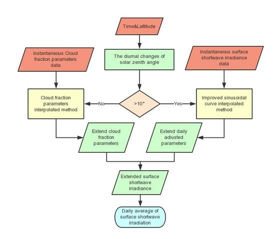
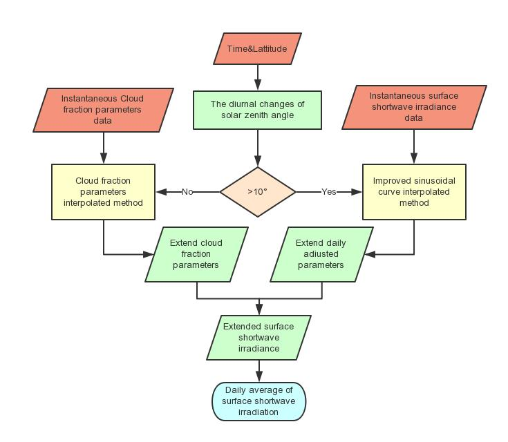
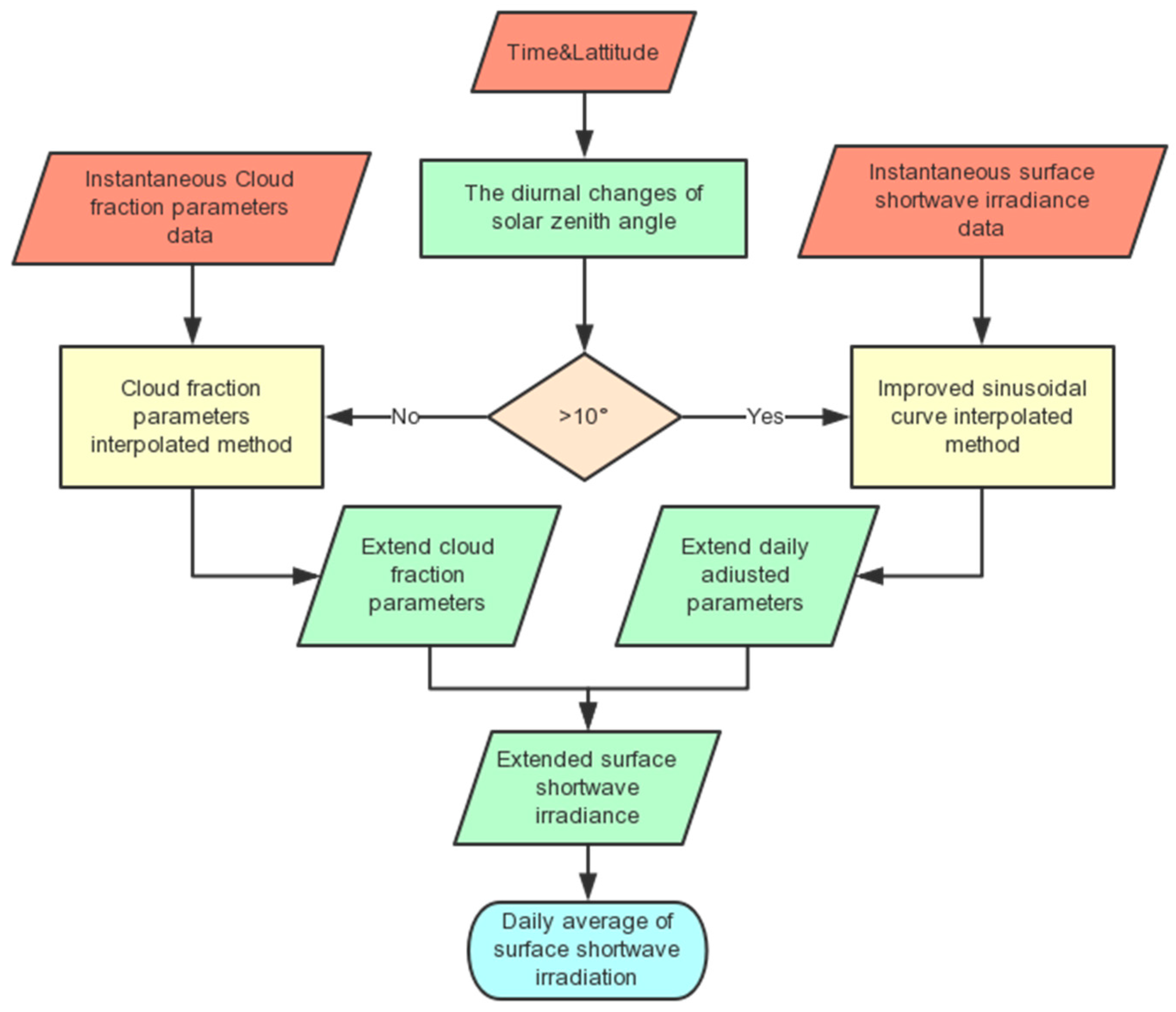
2.2. Temporal Scaling-Up Method

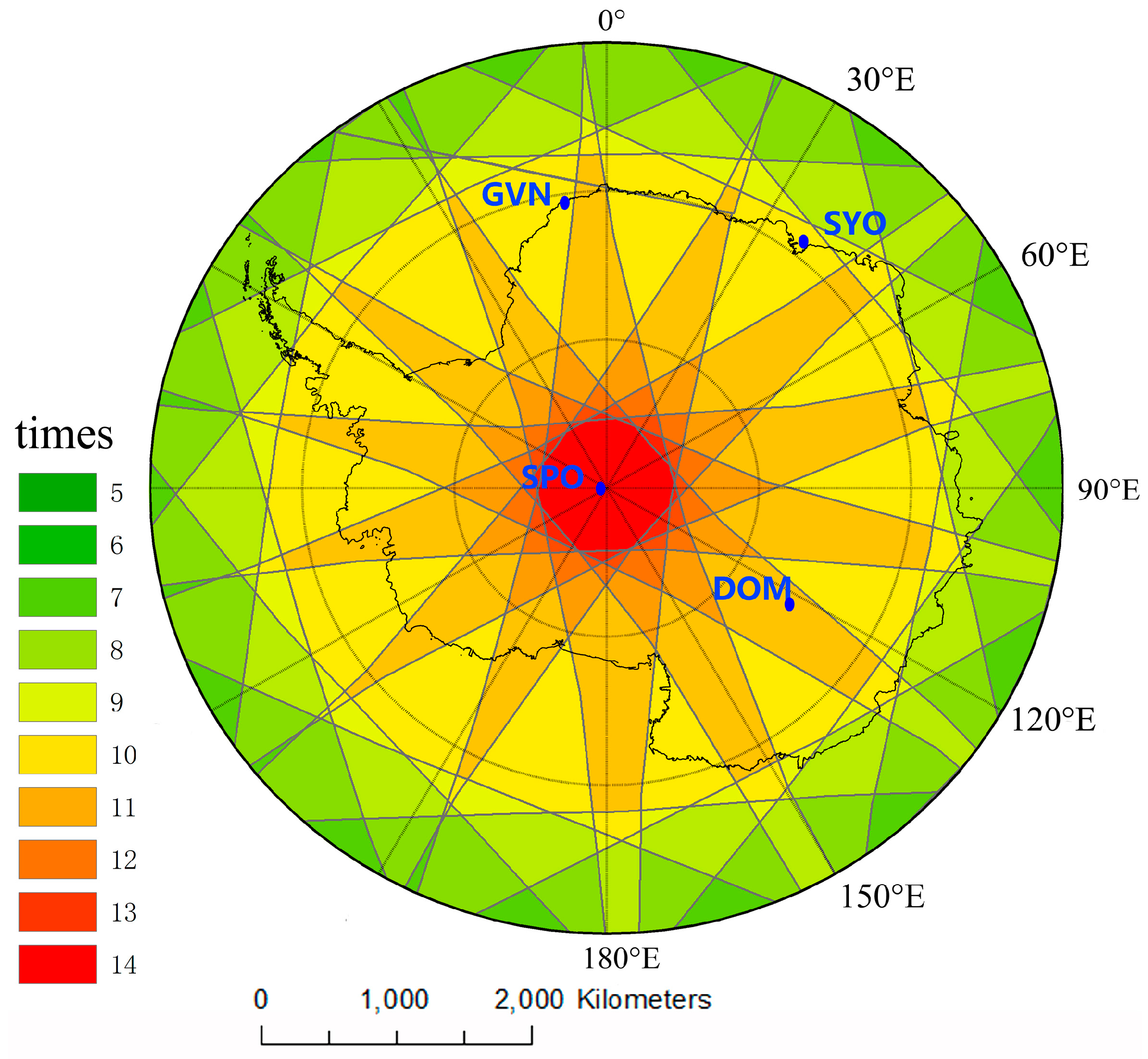
2.2.1. Calculation of the Diurnal Variation Range of SZA

In most areas, the diurnal variation in SZA is larger than 90°; it is the most important factor that affects downward shortwave irradiance [28]. The range of SZA diurnal variation is determined by latitude and date. We demonstrate the changes in DSR and SAZ on 17 October 2013 and 22 December 2013 at the GVN and SPO stations, respectively, to explain the diurnal variation in shortwave irradiance on the Antarctic surface in summer at different latitudes (shown in Figure 2).

The first step in our method is to calculate the range of diurnal SZA variation, sunrise time point and sunset time point [32]. Our sensitivity analysis indicates that if the range is larger than 10°, then SZA remains an important parameter when calculating radiation value. Consequently, we improve the sinusoidal method. If the change range is less than 10°, then cloud coverage becomes the most important influencing factor, which makes cloud coverage fraction interpolation a better choice.

2.2.2. Improved Sinusoidal Method

Traditional sinusoidal method firstly obtains satellite passing time point and the instantaneous irradiance value at this time point. Sunrise and sunset time points are then captured. The instantaneous values are determined with Formula (1) to calculate the maximum radiation in one day.

$$R_{n\_max}=\frac{R_{overpass}}{\sin \left(\frac{t_{overpass}-t_{rise}}{t_{set}-t_{rise}}\pi \right)}$$

(1)

The time point of satellite passing is marked as t_overpass, and the instantaneous value is marked as R_overpass. This formula leads to overestimated data of radiation because the SZA has small range of change in Antarctica. We improve this formula as Formula (2).

$$R_{n\_max}=\frac{R_{overpass}}{a\ast \sin \left[b\ast \left(\frac{t_{overpass}-t_{rise}}{t_{set}-t_{rise}}\right)\pi +c\right]+d}$$

(2)

A larger SZA in a high latitude area is considered, and parameter ‘a’ is inserted to compress the sine function. Downward irradiance is always positive during polar days; therefore, parameter ‘d’ is introduced to match the case. Parameters ‘b’ and ‘c’ are inserted to balance the different periods of time when SZA changes when compared with low-latitude areas. The curve can be fitted by least square method, after which the values of parameters ‘a,’ ‘b,’ ‘c’ and ‘d’ of each pixel in the area can be determined. The values of ‘a,’ ‘b,’ ‘c’, and ‘d’ are input into Formula (3), and we can obtain the irradiance value at any time in one day.

$$R_t=R_{overpass}\ast \frac{a\ast \sin \left[b\ast \left(\frac{\mathrm{t}-t_{rise}}{t_{set}-t_{rise}}\right)\pi +c\right]+d}{a\ast \sin \left[b\ast \left(\frac{t_{overpass}-t_{rise}}{t_{set}-t_{rise}}\right)\pi +c\right]+d}$$

(3)

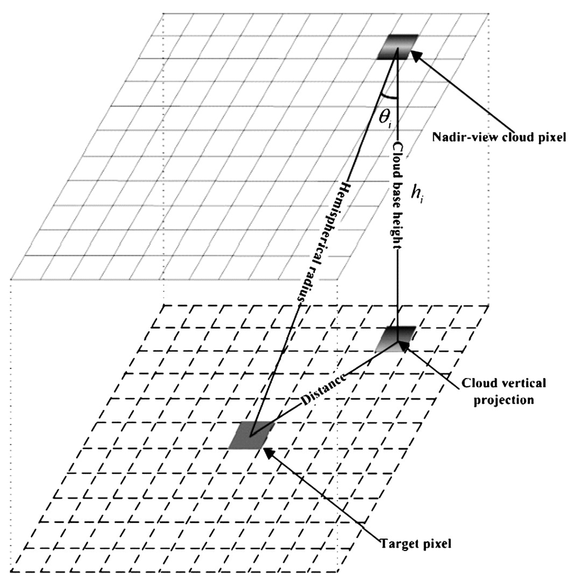
2.2.3. Cloud Coverage Fraction Interpolated Method

The improved sine curve model can match the case in most Antarctic areas, except near the South Pole. In this area, the daily change in SZA is insignificant. Instead, the main element that impacts downward shortwave irradiance is the cloud change. In our previous study, the most sensitive cloud parameters for irradiance estimation are HECF, COT, and RCF [28,33]. Consequently, we use satellite data to calculate instantaneous parameters to generate accurate data in this area. Other values at different times can be calculated with Formula (4).

$$\mathrm{P}\left(t\right)=\frac{t_{i+1}-t}{t_{i+1}-t_i}\ast \mathrm{P}\left(t_i\right)+\frac{t-t_i}{t_{i+1}-t_i}\ast \mathrm{P}\left(t_{i+1}\right)$$

(4)

‘t’ is the time point between two overpass times, when the latest polar-orbiting satellite overpass time is ’t_i’ and the next overpass time is ‘t_i+1’, ‘P(t)’ is the cloud parameter value at time ‘t’, and ‘P(t_i)’, ‘P(t_i+1)’ are the values at overpass time. We can let ’t’ to represent 24 h in one day.

We can then calculate the hourly downward shortwave irradiance flux by SBDART-CF model. In this way, the daily change in downward irradiance in this area can be revealed accurately.

2.2.4. Modelling Daily Solar Radiation

The process of calculating daily average downward shortwave irradiation values is described in Figure 3. The interpolation based on the improved sinusoidal method can integrate the values of irradiance from sunrise to sunset (00:00 to 24:00 during polar day) with Formula (5).

$$R_{daily}={{\displaystyle \int }}_{t_{rise}}^{t_{set}}{R}_t\left(t\right)dt$$

(5)

The cloud coverage fraction interpolated method can calculate the total radiation using Formula (6).

$$\begin{array}{l}{R}_{daily}={{\displaystyle \int }}_{t_{rise}}^{t_1}{R}_{t1}\left(t\right)dt\\ +{\displaystyle \sum _{i=1}^{n-1}}\left\{{{\displaystyle \int }}_{t_i}^{t_{i+1}}\left[\frac{t_{i+1}-t}{t_{i+1}-t_i}\ast R_{t_i}\left(t\right)+\frac{t-t_i}{t_{i+1}-t_i}\ast R_{t_i}\left(t\right)\right]dt\right\}\\ +{{\displaystyle \int }}_{t_n}^{t_{set}}{R}_{t_n}\left(t\right)dt\end{array}$$

(6)

We obtain hourly instantaneous values, and the other values between two instantaneous values are calculated with weighted average method. The daily average value can be estimated with Formula (7).

$$R_{daily\_avg}=R_{daily}/\left(t_{set}-t_{rise}\right)$$

(7)

3. Results

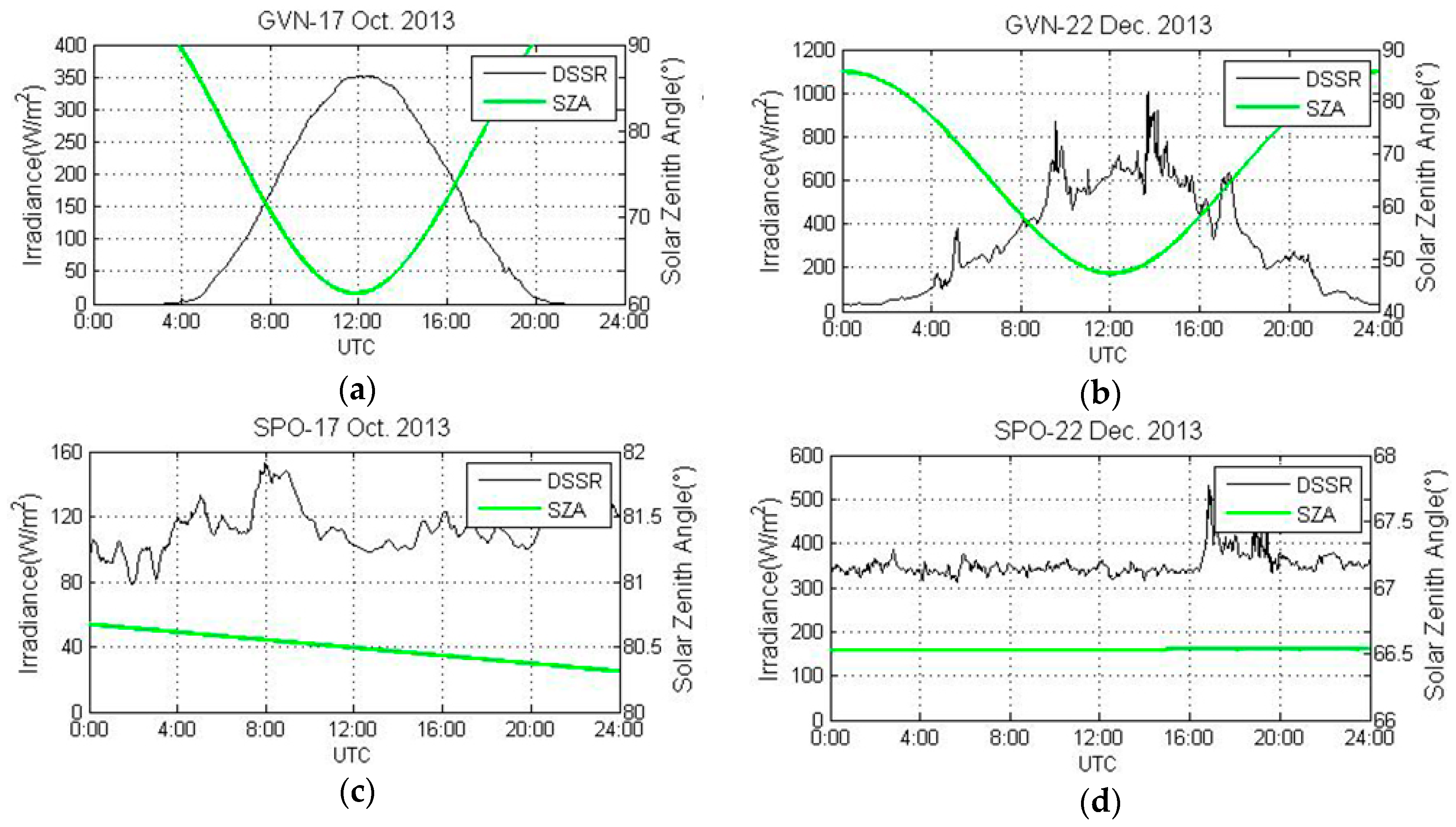
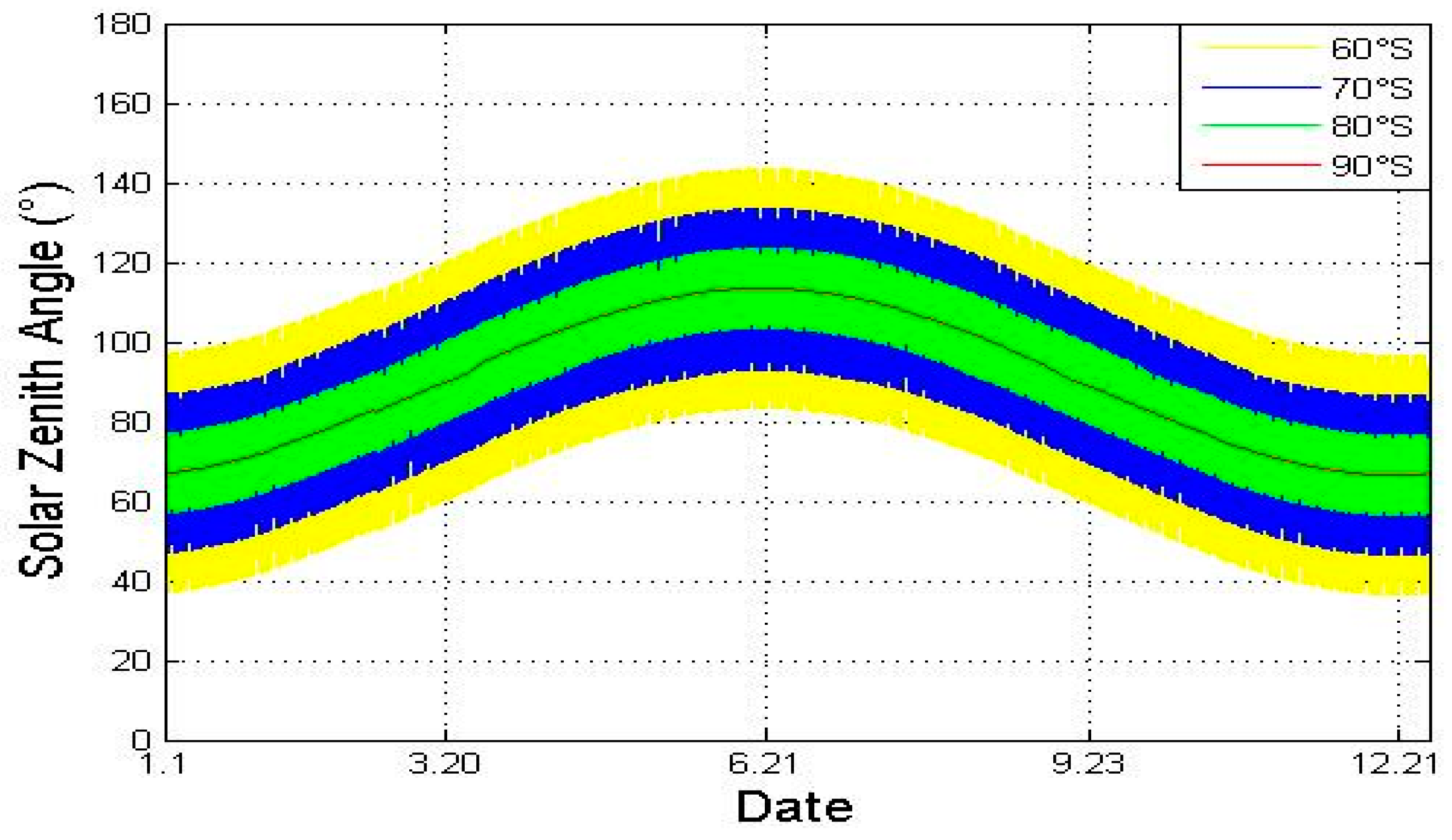
3.1. Diurnal Variation in SZA

We can calculate the diurnal variation in SZA at different dates and latitudes. During one year, the polar days and nights alternately show up in the southern hemisphere high-latitude area. We can calculate the range of SZA in one day on the basis of dates and latitudes. We can then decide which method should be used in specific area and date. Figure 4 shows the SZA change through the year at latitudes of 60°S, 70°S, 80°S, and 90°S.

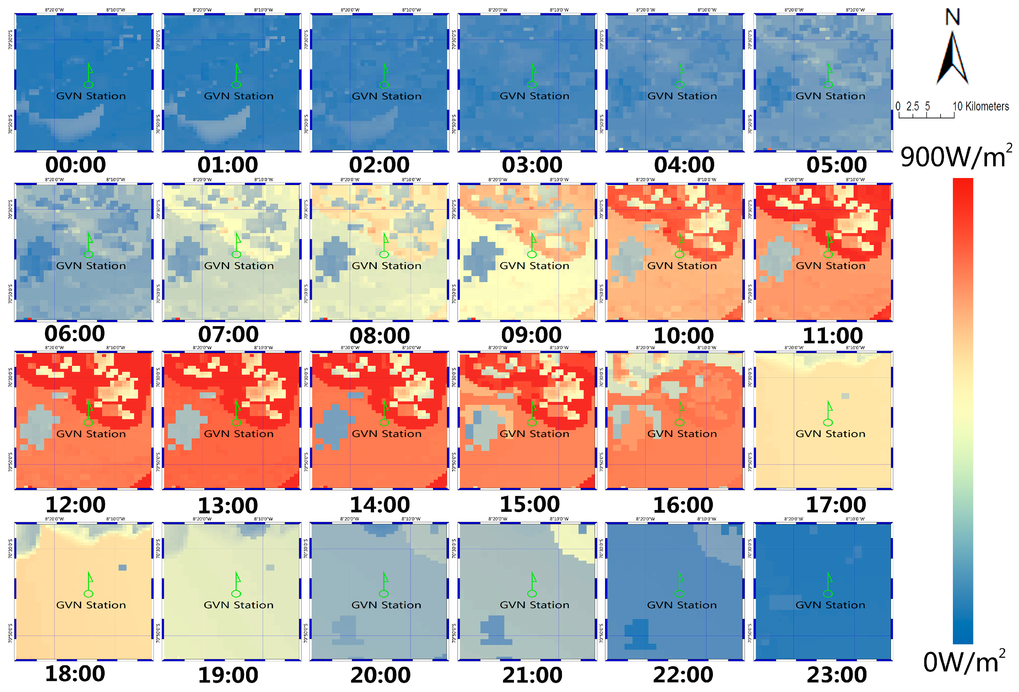
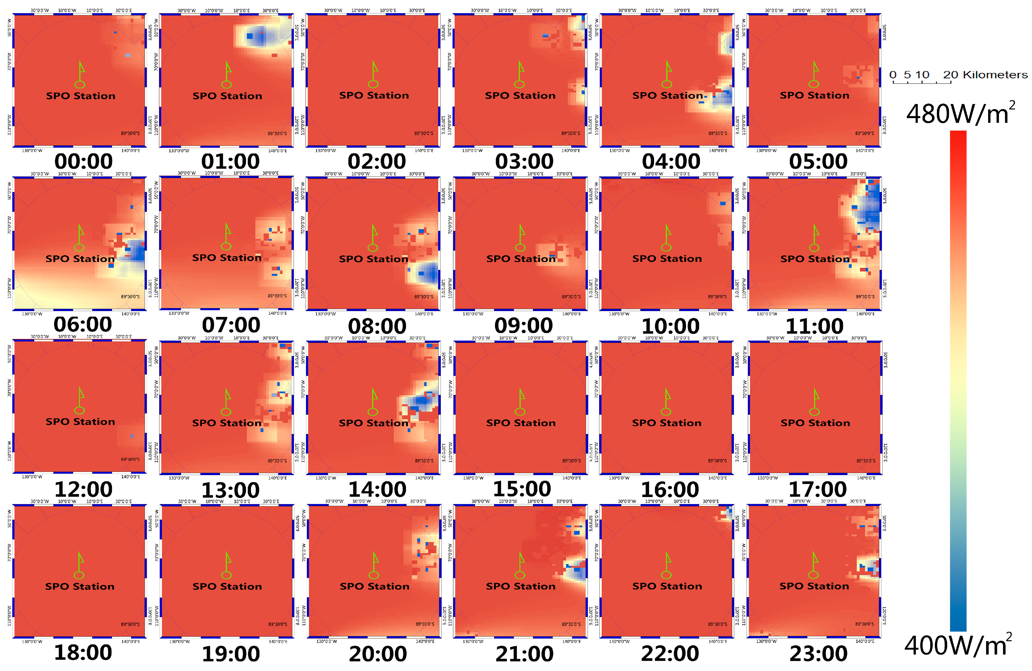
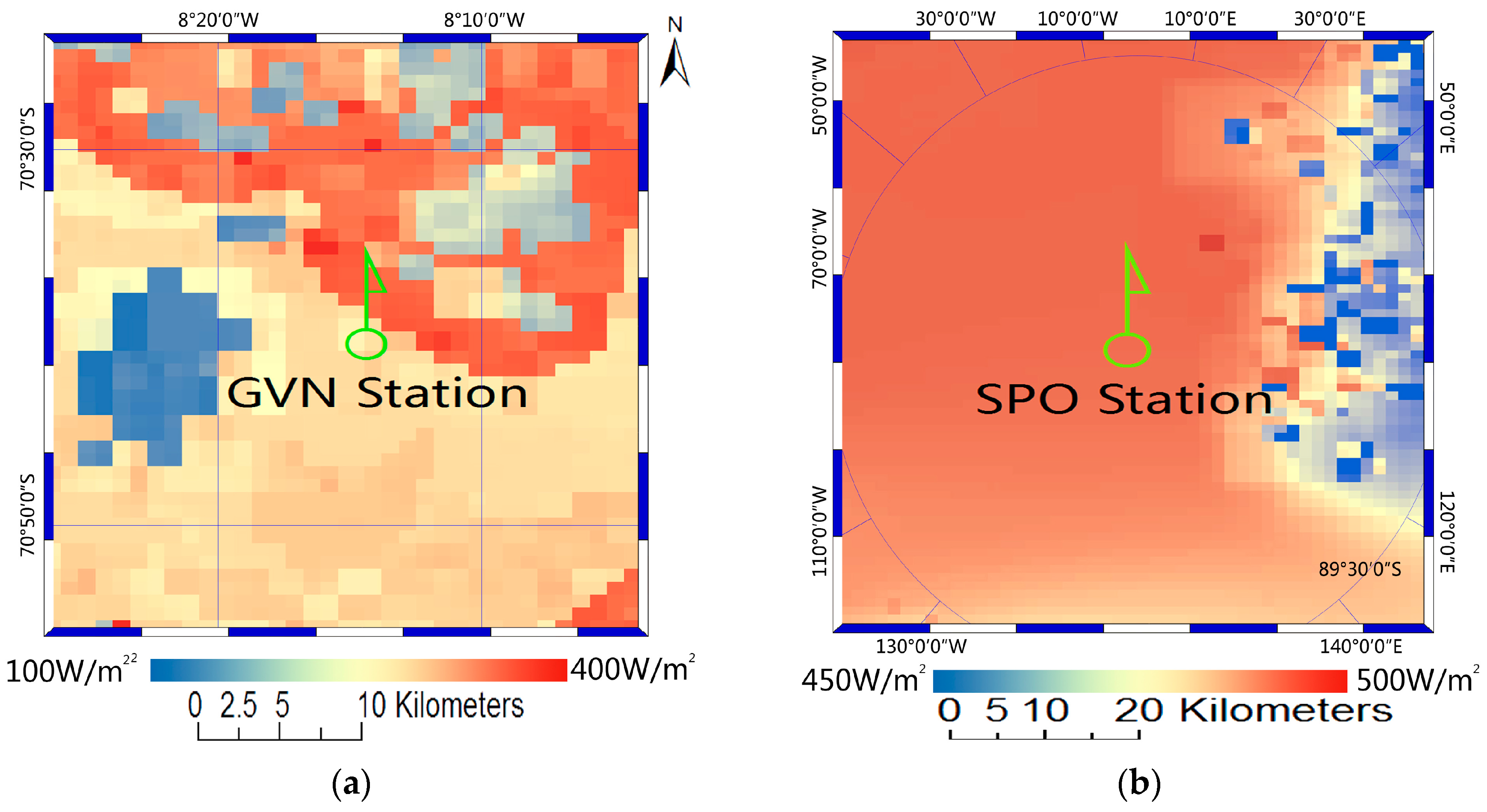
3.2. Diurnal Cycle of Interpolated Irradiance at Different Stations

The areas around the GVN and SPO stations are taken as examples. The diurnal variation in instantaneous downward shortwave irradiance estimated by two interpolation methods is shown below.

The interpolation results of the area around the GVN station are shown in Figure 5. Midnight sun occurs at the GVN station on that day; thus, the shortwave downward irradiance has a positive value over the entire 24-h period. Eight times of S-NPP transiting and corresponding products in the day at 0:47, 02:33, 14:32, 16:09, 17:15, 19:28, 21:10, and 22:47 are available. Although only 24 values are shown, the sinusoidal method can generate the irradiance value at any time in a day.

The shortwave irradiance around the GVN station shows a significant sinusoidal variation in one day. The maximum value appears near 14:00, and the values in the morning and evening are obviously lower. The lowest value is approximately 30 W/m², which matches the value that was measured by the GVN ground station.

Figure 6 shows the diurnal cycle results of surface shortwave irradiance where the SPO station is located. The cloud coverage parameter interpolation on 2 January 2015, indicates that the SPO station has 10 cloud parameter products on this day, and the satellite transit times are 0:03, 01:45, 03:22, 05:04, 06:47, 08:29, 11:54, 13:31, 18:38, and 22:03. The shortwave irradiance is stable around the SPO station, which is between 400 and 480 W/m². In fact, the more times the satellite can transit, the closer to actual situations the simulation cloud movement condition can be. On the contrary, when the satellite transits less, the insufficient consideration of temporal and spatial changes in clouds will lead to error.

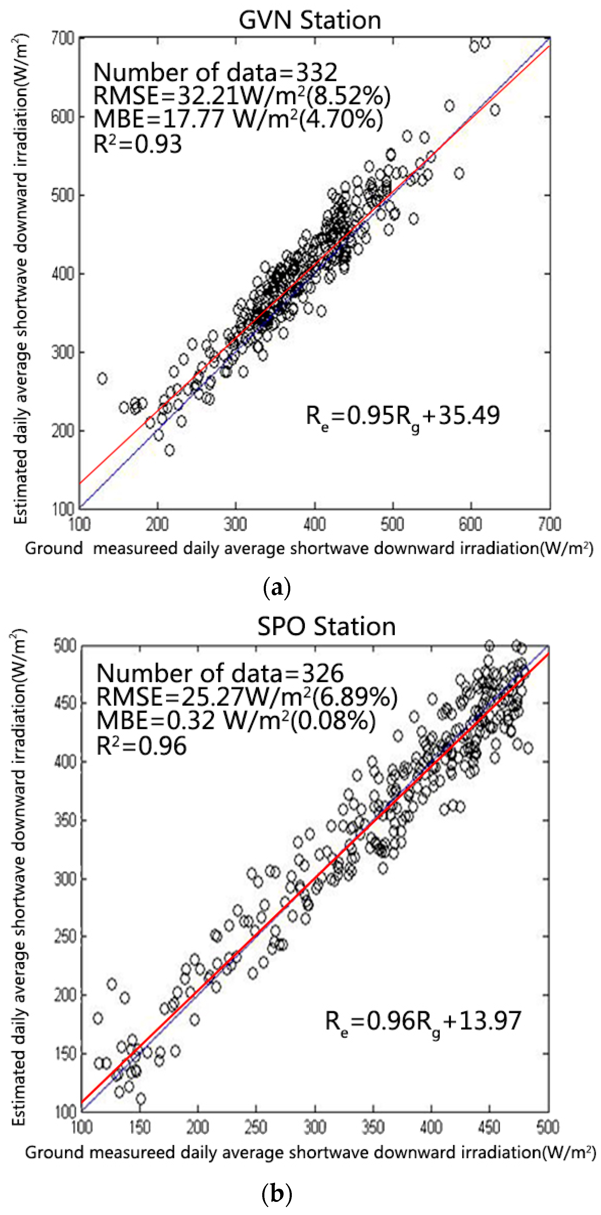
3.3. Average Daily Irradiation at Different Stations

We can calculate the total irradiation value of a day around the ground station with Formula (5) or (6) (shown in Figure 7). In polar days, we consider the length of day as 24 h; in other days, we can obtain the time points of sunrise and sunset [32]. Theoretically, the higher the temporal resolution of the instantaneous irradiance is, the more accurate the daily total and daily average values can be.

We use the data from December 2013 to February 2014, from December 2014 to February 2015, from December 2015 to February 2016, and from December 2016 to January 2017 to validate our estimated daily average values. The data quality control process is performed before validation to ensure that invalid data are deleted. We filter the data for SZA less than 90° and delete values that are less than zero. The measured value for some time periods is 0, which may be due to the snow cover being caused on the instrument surface. The irradiance values for these periods are also removed. We calculated the interpolation values in the neighbouring pixel (10 km × 10 km) and the daily average values measured by the ground station in summer are compared and analyzed. After data control, the number of daily average value in the SPO station is 326, and that in the GVN station is 332. In the formulas below, the ground-observed daily average irradiation data will be noted as R_O, and the estimated daily average irradiation data will be noted as R_e. The mean values of the two distributions are noted as R_Om and R_em. The total number of data is noted as N. Three statistical metrics are used to evaluate the estimates: the coefficient of determination (R²) calculated by Formula (8); the root mean square error (RMSE), as calculated by Formulas (9) and (10) and Mean bias error (MBE) calculated by Formulas (11) and (12) [34,35,36,37]. The RMSE and MBE are expressed here both in percent and absolute unit, as shown in Figure 8. The red line demonstrates the equation which includes Re and Rg, while the blue line is the demonstration when ‘Re = Rg’ for comparison.

$${\mathrm{R}}^2={\left[\frac{{{\displaystyle \sum }}_1^N\left(R_e-R_{em}\right)\ast \left(R_g-R_{gm}\right)}{{{\displaystyle \sum }}_1^N{\left(R_e-R_{em}\right)}^2\ast {\left(R_g-R_{gm}\right)}^2}\right]}^2$$

(8)

$$\mathrm{RMSE}=\sqrt[2]{\frac{{{\displaystyle \sum }}_1^N{\left(R_e-R_g\right)}^2}{N}}$$

(9)

$$\mathrm{RMSE}(\%)=\frac{100}{R_{gm}}\sqrt[2]{\frac{{{\displaystyle \sum }}_1^N{\left(R_e-R_g\right)}^2}{N}}$$

(10)

$$\mathrm{MBE}=\frac{{{\displaystyle \sum }}_1^N\left(R_e-R_g\right)}{N}$$

(11)

$$\mathrm{MBE}(\%)\frac{100}{R_{gm}}\ast \frac{{{\displaystyle \sum }}_1^N\left(R_e-R_g\right)}{N}$$

(12)

4. Discussion

4.1. Comparison of the Algorithm of the National Aeronautics and Space Administration (NASA)’s Surface Solar Radiation Budget Data Set

The U.S. NASA’s Surface Solar Radiation budget data set (https://gewex-srb.larc.nasa.gov/) produced for the Global Energy and Water Exchanges Programme provides daily average shortwave (SW) downward solar irradiation flux starting no later than July 1983 and extending to December 2007. SW surface radiation budget data sets are derived on a 1° × 1° global grid with two sets of algorithms, known as primary SW algorithm and Langley parameterized SW algorithms (LPSA) [38,39].

The primary SW algorithm gains irradiances from logarithmically averaged three-hourly International Satellite Cloud Climatology Project data. The satellite configuration consists of five geostationary satellites and at least one polar-orbiting satellite. The measurements taken at 00:00, 03:00, 06:00, 09:00, 12:00, 15:00, 18:00, and 21:00 UTC are included. The daily average irradiation is averaged by them. The LPSA using the values of daily average irradiation is computed by averaging measured daytime instantaneous (3 h) reflectance, weighted by the instantaneous value of cos SZA.

4.2. Comparison with Traditional Interpolation Methods

We intend to use two different interpolation methods to obtain the daily average values with high accuracy of DSSR in the study area. In 1979, Tarpley indicated that the sinusoidal formula of the SZA can be used to approximate the daily variation IN solar radiation [19]. The diurnal variation in surface shortwave irradiance is not a simple sinusoidal model due to geographical location, atmospheric conditions, and other factors, which means that the model needs to be corrected.

Lagouarde and Brunet advanced a sinusoidal model that can describe the diurnal variation in surface temperature and considers the time span and amplitude of curve [20]. Bisht proposed a diurnal sinusoidal model of surface net radiation, which is suitable for interpolation with MODIS data under clear sky conditions [18]. Wang proposed a modified sinusoidal method, supposing the values of irradiance at sunrise and sunset are zero [23]. However, the curve amplitude is smaller due to the smaller diurnal variation in SZA in Antarctica. In addition, no sunrise or sunset exists due to the polar day in summer, which makes the curve time span longer, even one cycle longer than the traditional curve. We set parameters ‘a’ and ‘d’ to adjust the curve amplitude in Formula (2), and parameters ‘b’ and ‘c’ to control time span and cycle.

The transit time is more than four in one day; therefore, we can set four parameters to adjust the sinusoidal curve.

Table 2. Comparison between the daily average values estimated by four different interpolation methods and ground measurements from two stations.

Station	Method	R2	C1 (W/m2)	C2	RMSE (W/m2)	RMSE (%)	MBE (W/m2)	MBE (%)
GVN station	Improved sinusoidal curve	0.93	35.49	0.95	32.21	8.52	17.77	4.70
	Traditional sinusoidal curve	0.68	55.50	1.09	70.32	18.59	36.39	9.62
SPO station	Cloud coverage fraction Interpolation	0.96	13.97	0.96	25.27	6.98	0.32	0.08
	Linear interpolation	0.79	28.51	1.04	57.40	15.87	30.18	8.34

shows the estimated daily average downward shortwave irradiation based on the traditional sinusoidal curve (the R² is near 0.68, and the RMSE is 70.32 W/m²). The parameters of the linear fits R_e = C₁+ C₂ × R_g for the two methods in the GVN station are also shown in Table 2.

In Antarctica, the sensitivity analysis method is used to prove that the cloud coverage fraction is the main parameter when diurnal changes in SZA are small. Unlike in the linear interpolation method, whether interpolation or calculation should be performed firstly does not matter in the cloud coverage fraction interpolation. In our calculations, the relationship between cloud coverage and downward shortwave irradiance values in the SBDART-CF model is nonlinear, which leads to different results. Table 2 shows the results from the linear interpolation method. If cloud coverage does not change over time, the results of two methods should be similar. Therefore, the cloud coverage interpolation method is more suitable when the cloud cover changes. The parameters of the linear fits R_e = C₁+ C₂ × R_g for the two methods in SPO station are shown in Table 2.

4.3. Limitation and Further Study

In Figure 5, the DSR is not continuous in space, because when we fit the four parameters, the influence of the cloud is ignored in some areas and enlarged in other areas. An apparent disadvantage of the sinusoidal method is that the cloud coverage in every transmit time will affect the four parameters in Formula (2).

In Figure 8a, the results of daily average irradiation values are slightly overestimated. In the experiments, the changes of irradiance near the station are not only caused by the change of SZA, but also by cloud conditions. Consequently, this method is more suitable under clear sky conditions. We need more cloud data from polar satellite to capture the change of cloud. S-NPP is the only satellite on which this paper relies. Obtaining data from more satellites can reduce the error between the interpolation results and the real-time measured values.

The cloud coverage interpolation method is computationally intensive and inefficient. With the accumulation of future cloud data, a look-up table between cloud coverage changes and the DSR in this area can be established to speed up the operation.

The methods of this study are not suitable for low and middle latitude areas because of inadequate satellite transits. However, the fusion of multi-source orbit satellite cloud data can cover the shortage of inadequate transits to some extent. Thus, the high spatial resolution geostationary satellite will be helpful in making our methods suitable for lower latitude areas [40,41].

More profound problems must be solved in the future. Firstly, the terrain effect in the research area is not considered in this paper. The influence of different topography on downward shortwave irradiance in Antarctica should be considered in further studies when combined with our previous studies [42]. Secondly, the influence of surface weather conditions is ignored owing to the lack of the surface weather data. Thirdly, the data for interpolation are available only after 2013 because of the limitation of the satellite launch time. In further studies, AVHRR and MODIS satellite sensors can be used [43], and the surface shortwave radiation estimate data set with long-term data series based on the method that is provided in this paper can be established.

5. Conclusions

In this paper, two interpolation methods to estimate daily average values of downward shortwave irradiation are mainly discussed. On the basis of the sinusoidal method provided by previous research, this research has improved the traditional sinusoidal interpolation method. Meanwhile, we present new cloud fraction parameter interpolation method to consider the cloud condition change in Antarctica. Four parameters are introduced (‘a’, ‘b’, ‘c’ and ‘d’) and are fitted in the improved sinusoidal method, with the data support of the S-NPP satellite that passes through polar areas several times a day. In this manner, the traditional sine curve model is improved to prevent overestimation. For cloud coverage fraction parameter interpolation method, the S-NPP satellite cloud product provides cloud fraction data of the hemisphere space, which are the input parameters to obtain the interpolation results.

According to the validation by the data from two BSRN surface stations, the R² of the first method is 0.93; the RMSE is 32.21 W/m² (8.52%) and the MBE is 17.77 W/m² (4.70%) in GVN station area. The R², RMSE and MBE of the second method are 0.96, 25.27 W/m² (6.98%) and 0.32 W/m² (0.08%), respectively, in the SPO station area. When compared with existing methods, our methods are more accurate than the traditional sinusoidal method (R² = 0.68; RMSE = 70.32 W/m² (18.59%) and MBE = 36.39 W/m² (9.62%)) in GVN station area and the direct linear interpolation method (R² = 0.79; RMSE = 57.40 W/m² (15.87%); MBE = 38.18 W/m² (8.34%)) in SPO station area.

References

1. Platt, T. Primary production of the ocean water column as a function of surface light intensity: Algorithms for remote sensing. Deep Sea Res. Part A Oceanogr. Res. Pap. 1986, 33, 149–163. [Google Scholar] [CrossRef]
2. Shook, K.; Pomeroy, J. Synthesis of incoming shortwave radiation for hydrological simulation. Hydrol. Res. 2011, 42, 433–446. [Google Scholar] [CrossRef]
3. Wild, M.; Ohmura, A.; Schär, C.; Müller, G.; Folini, D.; Schwarz, M.; Hakuba, M.Z.; Sanchez-Lorenzo, A. The global energy balance archive (GEBA) version 2017: A database for worldwide measured surface energy fluxes. Earth Syst. Sci. Data 2017, 9, 601. [Google Scholar] [CrossRef]
4. Budyko, M.I. The effect of solar radiation variations on the climate of the earth. Tellus 1969, 21, 611–619. [Google Scholar] [CrossRef]
5. Kiehl, J.T.; Trenberth, K.E. Earth’s annual global mean energy budget. Bull. Am. Meteorol. Soc. 1997, 78, 197–208. [Google Scholar] [CrossRef]
6. Foukal, P.; Fröhlich, C.; Spruit, H.; Wigley, T. Variations in solar luminosity and their effect on the earth’s climate. Nature 2006, 443, 161–166. [Google Scholar] [CrossRef] [PubMed]
7. Hansom, J.D.; Gordon, J. Antarctic Environments and Resources: A Geographical Perspective; Routledge: New York, NY, USA; Oxfordshire, UK, 2014. [Google Scholar]
8. Hall, A. The role of surface albedo feedback in climate. J. Clim. 2004, 17, 1550–1568. [Google Scholar] [CrossRef]
9. Holland, M.M.; Bitz, C.M. Polar amplification of climate change in coupled models. Clim. Dyn. 2003, 21, 221–232. [Google Scholar] [CrossRef]
10. Stanhill, G.; Cohen, S. Recent changes in solar irradiance in Antarctica. J. Clim. 1997, 10, 2078–2086. [Google Scholar] [CrossRef]
11. King, J.; Connolley, W. Validation of the surface energy balance over the antarctic ice sheets in the UK meteorological office unified climate model. J. Clim. 1997, 10, 1273–1287. [Google Scholar] [CrossRef]
12. Stocker, T. Climate Change 2013: The Physical Science Basis: Working Group I Contribution to the Fifth Assessment Report of the Intergovernmental Panel on Climate Change; Cambridge University Press: Cambridge, UK, 2014. [Google Scholar]
13. Wild, M.; Folini, D.; Henschel, F.; Fischer, N.; Müller, B. Projections of long-term changes in solar radiation based on cmip5 climate models and their influence on energy yields of photovoltaic systems. Sol. Energy 2015, 116, 12–24. [Google Scholar] [CrossRef]
14. Trnka, M.; Žalud, Z.; Eitzinger, J.; Dubrovský, M. Global solar radiation in central European lowlands estimated by various empirical formulae. Agric. For. Meteorol. 2005, 131, 54–76. [Google Scholar] [CrossRef]
15. Journée, M.; Bertrand, C. Improving the spatio-temporal distribution of surface solar radiation data by merging ground and satellite measurements. Remote Sens. Environ. 2010, 114, 2692–2704. [Google Scholar] [CrossRef]
16. Pinker, R.; Frouin, R.; Li, Z. A review of satellite methods to derive surface shortwave irradiance. Remote Sens. Environ. 1995, 51, 108–124. [Google Scholar] [CrossRef]
17. Liang, S.; Zheng, T.; Liu, R.; Fang, H.; Tsay, S.C.; Running, S. Estimation of incident photosynthetically active radiation from moderate resolution imaging spectrometer data. J. Geophys. Res. Atmos. 2006, 111. [Google Scholar] [CrossRef]
18. Bisht, G.; Venturini, V.; Islam, S.; Jiang, L. Estimation of the net radiation using modis (moderate resolution imaging spectroradiometer) data for clear sky days. Remote Sens. Environ. 2005, 97, 52–67. [Google Scholar] [CrossRef]
19. Tarpley, J. Estimating incident solar radiation at the surface from geostationary satellite data. J. Appl. Meteorol. 1979, 18, 1172–1181. [Google Scholar] [CrossRef]
20. Lagouarde, J.; Brunet, Y. A simple model for estimating the daily upward longwave surface radiation flux from noaa-avhrr data. Int. J. Remote Sens. 1993, 14, 907–925. [Google Scholar] [CrossRef]
21. Van Laake, P.E.; Sanchez-Azofeifa, G.A. Mapping par using modis atmosphere products. Remote Sens. Environ. 2005, 94, 554–563. [Google Scholar] [CrossRef]
22. Niu, X. Radiative Fluxes and Albedo Feedback in Polar Regions; University of Maryland: College Park, MD, USA, 2011. [Google Scholar]
23. Wang, D.; Liang, S.; Liu, R.; Zheng, T. Estimation of daily-integrated par from sparse satellite observations: Comparison of temporal scaling methods. Int. J. Remote Sens. 2010, 31, 1661–1677. [Google Scholar] [CrossRef]
24. Xu, X.; Du, H.; Zhou, G.; Mao, F.; Li, P.; Fan, W.; Zhu, D. A method for daily global solar radiation estimation from two instantaneous values using modis atmospheric products. Energy 2016, 111, 117–125. [Google Scholar] [CrossRef]
25. Chen, L.; Yan, G.; Ren, H.; Wang, T. A simple fusion algorithm of polar-orbiting and geostationary satellite data for the estimation of surface shortwave fluxes. In Proceedings of the 2016 IEEE International Geoscience and Remote Sensing Symposium (IGARSS), Beijing, China, 10–15 July 2016; IEEE: Piscataway, NJ, USA, 2016; pp. 2657–2660. [Google Scholar]
26. Cao, C.; De Luccia, F.J.; Xiong, X.; Wolfe, R.; Weng, F. Early on-orbit performance of the visible infrared imaging radiometer suite onboard the suomi national polar-orbiting partnership (s-npp) satellite. IEEE Trans. Geosci. Remote Sens. 2014, 52, 1142–1156. [Google Scholar] [CrossRef]
27. Yan, K.; Park, T.; Chen, C.; Xu, B.; Song, W.; Yang, B.; Zeng, Y.; Liu, Z.; Yan, G.; Knyazikhin, Y.; et al. Generating global products of lai and fpar from snpp-viirs data: Theoretical background and implementation. IEEE Trans. Geosci. Remote Sens. 2018, PP, 1–19. [Google Scholar] [CrossRef]
28. Zhao, J.; Yan, G.; Jiao, Z.; Chen, L.; Chu, Q. Enhanced shortwave radiative transfer model based on sbdart. J. Remote Sens. 2017, 6, 853–863. [Google Scholar]
29. König-Langlo, G.; Sieger, R.; Schmithüsen, H.; Bücker, A.; Richter, F.; Dutton, E. The Baseline Surface Radiation Network and Its World Radiation Monitoring Centre at the Alfred Wegener Institute; World Meteorological Organization: Geneva, Switzerland, 2013. [Google Scholar]
30. König-Langlo, G.; Loose, B. The meteorological observatory at neumayer stations (gvn and nm-ii) Antarctica. Polarforschung2006 2007, 76, 25–38. [Google Scholar]
31. Dutton, E.G. Basic and other measurements of radiation at station south pole (1998-06). Earth Environ. Sci. 2007. [Google Scholar] [CrossRef]
32. Grena, R. An algorithm for the computation of the solar position. Sol. Energy 2008, 82, 462–470. [Google Scholar] [CrossRef]
33. Chen, L.; Yan, G.; Wang, T.; Ren, H.; Calbó, J.; Zhao, J.; McKenzie, R. Estimation of surface shortwave radiation components under all sky conditions: Modeling and sensitivity analysis. Remote Sens. Environ. 2012, 123, 457–469. [Google Scholar] [CrossRef]
34. Gueymard, C.A. A review of validation methodologies and statistical performance indicators for modeled solar radiation data: Towards a better bankability of solar projects. Renew. Sustain. Energy Rev. 2014, 39, 1024–1034. [Google Scholar] [CrossRef]
35. Román, R.; Antón, M.; Valenzuela, A.; Gil, J.; Lyamani, H.; De Miguel, A.; Olmo, F.; Bilbao, J.; Alados-Arboledas, L. Evaluation of the desert dust effects on global, direct and diffuse spectral ultraviolet irradiance. Tellus B Chem. Phys. Meteorol. 2013, 65, 19578. [Google Scholar] [CrossRef]
36. Mateos, D.; Bilbao, J.; Kudish, A.; Parisi, A.; Carbajal, G.; Di Sarra, A.; Román, R.; De Miguel, A. Validation of omi satellite erythemal daily dose retrievals using ground-based measurements from fourteen stations. Remote Sens. Environ. 2013, 128, 1–10. [Google Scholar] [CrossRef] [Green Version]
37. De Miguel-Bilbao, S.; Ramos, V.; Blas, J. Assessment of polarization dependence of body shadow effect on dosimetry measurements in 2.4 ghz band. Bioelectromagnetics 2017, 38, 315–321. [Google Scholar] [CrossRef] [PubMed]
38. Pinker, R.; Laszlo, I. Modeling surface solar irradiance for satellite applications on a global scale. J. Appl. Meteorol. 1992, 31, 194–211. [Google Scholar] [CrossRef]
39. Gupta, S.K.; Kratz, D.P.; Stackhouse, P.W., Jr.; Wilber, A.C. The Langley Parameterized Shortwave Algorithm (LPSA) for Surface Radiation Budget Studies; version 1.0; Langley Research Center: Hampton, VA, USA, 2001.
40. Yang, J.; Zhang, Z.; Wei, C.; Lu, F.; Guo, Q. Introducing the new generation of Chinese geostationary weather satellites–fengyun 4 (fy-4). Bull. Am. Meteorol. Soc. 2016. [CrossRef]
41. Bessho, K.; Date, K.; Hayashi, M.; Ikeda, A.; Imai, T.; Inoue, H.; Kumagai, Y.; Miyakawa, T.; Murata, H.; Ohno, T. An introduction to himawari-8/9—Japan’s new-generation geostationary meteorological satellites. J. Meteorol. Soc. Jpn. Ser. II 2016, 94, 151–183. [Google Scholar] [CrossRef]
42. Yan, G.; Wang, T.; Jiao, Z.; Mu, X.; Zhao, J.; Chen, L. Topographic radiation modeling and spatial scaling of clear-sky land surface longwave radiation over rugged terrain. Remote Sens. Environ. 2016, 172, 15–27. [Google Scholar] [CrossRef]
43. Jiao, Z.; Yan, G.; Zhao, J.; Wang, T.; Chen, L. Estimation of surface upward longwave radiation from modis and viirs clear-sky data in the Tibetan plateau. Remote Sens. Environ. 2015, 162, 221–237. [Google Scholar] [CrossRef]
Figure 1. Overpass times of the Suomi National Polar-Orbiting Partnership satellite in one day and distribution of Baseline Surface Radiation Network stations in Antarctica.
Remotesensing 10 00422 g001
Figure 2. (a) Diurnal variation range of solar zenith angle (SZA) and downward surface shortwave irradiance (DSSR) at the Georg von Neumayer (GVN) station on 17 October 2013; (b) Diurnal variation range of SZA and DSSR at the GVN station on 22 December 2013; (c) Diurnal variation range of SZA and DSSR at the South Pole (SPO) station on 17 October 2013; and, (d) Diurnal variation range of SZA and DSSR at SPO station on 22 December 2013.
Remotesensing 10 00422 g002
Figure 3. Process of calculating daily average downward shortwave irradiation values.
Remotesensing 10 00422 g003
Figure 4. Change range of solar zenith angle at latitudes of 60°S, 70°S, 80°S, and 90°S in all year.
Remotesensing 10 00422 g004
Figure 5. Results of hourly interpolation in the Georg von Neumayer station area on 9 December 2014.
Remotesensing 10 00422 g005
Figure 6. Results of hourly interpolation in the South Pole station area on 2 January 2015.
Remotesensing 10 00422 g006
Figure 7. (a) Daily average value of solar global irradiation over horizontal surface in the Georg von Neumayer station area on 9 December 2014; and, (b) Daily average value of solar global irradiation over horizontal surface in the South Pole station area on 2 January 2015.
Remotesensing 10 00422 g007
Figure 8. (a) Comparison of the estimated downward shortwave irradiation from the improved sinusoidal method and the ground-measured downward shortwave irradiation in the Georg von Neumayer station; and, (b) Comparison of the estimated downward shortwave irradiation from the cloud coverage fraction interpolated method and the ground-measured downward shortwave irradiation in the South Pole station area.
Remotesensing 10 00422 g008