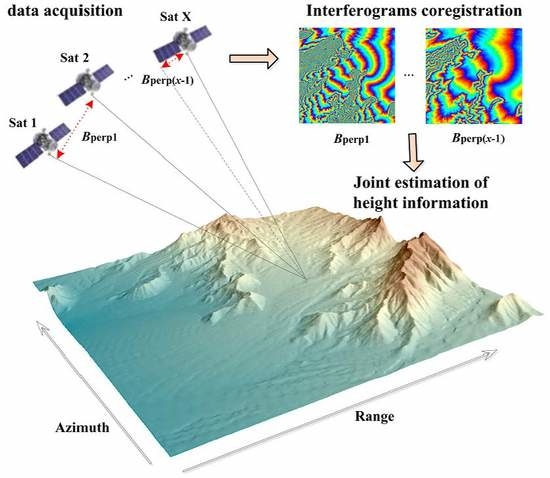
Article

An Efficient Maximum Likelihood Estimation Approach of Multi-Baseline SAR Interferometry for Refined Topographic Mapping in Mountainous Areas

1
State Key Laboratory of Information Engineering in Surveying, Mapping and Remote Sensing, Wuhan University, 129 Luoyu Road, Wuhan 430079, China
2
College of Geographic and Biologic Information, Nanjing University of Posts and Telecommunications, Nanjing 210023, China
3
Collaborative Innovation Center of Geospatial Technology, Wuhan University, 129 Luoyu Road, Wuhan 430079, China
*
Author to whom correspondence should be addressed.
Remote Sens. 2018, 10(3), 454; https://doi.org/10.3390/rs10030454
Submission received: 4 January 2018 / Revised: 23 February 2018 / Accepted: 5 March 2018 / Published: 14 March 2018
(This article belongs to the Special Issue Advances in SAR: Sensors, Methodologies, and Applications)

Abstract

:
For InSAR topographic mapping, multi-baseline InSAR height estimation is known to be an effective way to facilitate phase unwrapping by significantly increasing the ambiguity intervals and maintaining good height measurement sensitivity, especially in mountainous areas. In this paper, an efficient multi-baseline SAR interferometry approach based on maximum likelihood estimation is developed for refined topographic mapping in mountainous areas. In the algorithm, maximum likelihood (ML) height estimation is used to measure the topographic details and avoid the complicated phase unwrapping process. In order to be well-adapted to the mountainous terrain conditions, the prior height probability is re-defined to take the local terrain conditions and neighboring height constraint into consideration in the algorithm. In addition, three strategies are used to optimize the maximum likelihood height estimation process to obtain higher computational efficiency, so that this method is more suitable for spaceborne InSAR data. The strategies include substituting a rational function model into the complicated conversion process from candidate height to interferometric phase, discretizing the continuous height likelihood probability, and searching for the maximum likelihood height with a flexible step length. The experiment with simulated data is designed to verify the improvement of the ML height estimation accuracy with the re-defined prior height distribution. Then the optimized processing procedure is tested with the multi-baseline L-band ALOS/PALSAR data covering the Mount Tai area in China. The height accuracy of the generated multi-baseline InSAR DEM can meet both standards of American DTED-2 and Chinese national 1:50,000 DEM (mountain) Level 2.

Graphical Abstract

1. Introduction

SAR interferometry (InSAR) is an effective tool for large-area topographic mapping due to its all-weather imaging and high sensitivity to terrain relief [1,2]. The InSAR height measurement accuracy is greatly influenced by the phase unwrapping accuracy and the length of normal baselines [3,4]. Longer normal baselines allow more accurate height estimation but also generate higher frequency of the interferometric fringes, which increases the complexity of phase unwrapping. On the other hand, shorter normal baselines reduce the complexity of phase unwrapping but suffer from poorer phase-to-height sensitivity [5,6]. Therefore, the contradiction between the sensitivity of height measurement and the reliability of phase unwrapping caused by the length of normal baseline over rough terrain is inevitable for single-baseline InSAR.
To combine the advantages of large and short baselines in topographic mapping, a multi-baseline InSAR principle has been proposed to estimate terrain height by joint analysis of multiple interferometric pairs with diverse normal baselines [7,8]. Researchers have proposed a variety of methods for multi-baseline InSAR processing. The standard method to increase the accuracy of interferometric DEMs is to stack multiple geocoded layers, weighted with the individual error estimates [9,10,11]. However, all DEM stacking approaches assume correctly unwrapped interferograms. Moreover, it is difficult to co-register different geocoded DEM layers accurately and the horizontal displacements can introduce height errors. Other multi-baseline estimation methods have been published to facilitate the phase unwrapping process by taking advantage of baseline diversity, such as the Least Square estimation method [5], the iterative multi-baseline method [12], the Chinese Remainder Theorem (CRT) method [13,14], and so on. These multi-baseline phase unwrapping methods can significantly increase the ambiguity intervals of interferometric phases and keep the topographic details as well; however, these methods still have to solve the phase unwrapping problem correctly.
In order to avoid the phase unwrapping process and determine the target height directly, the statistical method using the criterion of maximum likelihood [9,15,16,17,18] is exploited to combine the multi-baseline information for target height estimation. However, in actual data processing, atmospheric effects, orbital errors, and decorrelation will introduce phase noise that cannot be ignored. Therefore, the maximum likelihood estimation method is not robust enough to search for the target height within all elevation values. In order to realize more robust and reliable height estimation, the prior height information from the reference DEM is incorporated into the ML estimation to restrict the height searching range [18], but the problem is that the local terrain conditions and the neighboring height constraint are not considered in the prior height distribution. The maximum a posteriori (MAP) estimation tries to introduce the neighboring height constraints by using Markov random fields to model the prior distribution of the unknown images [19,20]. This method allows recovering topographic profiles affected by strong height discontinuities and performing efficient noise rejections. However, the MAP methods also have limits concerning the computational time and the optimization step because there is no guarantee of finding the global optimum.
In this article, we apply the maximum likelihood estimation for multi-baseline InSAR DEM generation. The prior height probability is re-defined to take the local terrain conditions and neighboring height constraint into consideration. An experiment with simulated data is designed to verify the improvement of the ML height estimation accuracy with the well-defined prior height distribution. Furthermore, to make the maximum likelihood estimation method well adapted to spaceborne SAR data, the processing flow is optimized for higher computational efficiency with the following innovative points: (1) Replacing the rigorous height-to-phase conversion with the rational function model (RFM); (2) substituting the complicated height likelihood probability function with two-dimension lookup table; (3) searching for the maximum likelihood height with flexible search step length instead of fixed search step length. This processing flow is testified with the L-band ALOS/PALSAR data, which can be less influenced by the temporal and volume decorrelation and have a longer critical baseline than InSAR data with a shorter wavelength (such as X band or C band) [21]. Since the ALOS/PALSAR data were acquired in the repeat-pass mode, the above processing flow integrates atmospheric effect correction to improve the reliability of multi-baseline estimation. The rest of this article is structured as follows: Section 2 introduces the principle of ML estimation with prior DEM; Section 3 presents the improved proposed processing flow for spaceborne datasets; detailed descriptions of the experiments and results are given in Section 4; Section 5 is a discussion of the experimental results; finally, the conclusions are drawn.

2. Maximum Likelihood Height Estimation Assisted by Prior DEM

2.1. Basic Principle

The maximum likelihood (ML) height estimation method of multi-baseline InSAR considers the target height h as a parameter of the probability distribution of the interferometric phase ϕ , denoted as p d f ( ϕ | h ) , and combines the probability distributions of all the interferometric phase observations to estimate the target height with the maximum likelihood criterion [22]. Aiming at reducing the undesired variation in the maximum likelihood height estimation caused by non-negligible phase noise, the prior height distribution from a reference DEM is integrated into the maximum likelihood estimation, which not only greatly improves the estimation reliability but also narrows the search range and increases the computational efficiency. Therefore, the maximum likelihood height estimation assisted by the reference DEM is shown in Equation (1):
H ^ M L = arg   max h F { [ i = 1 K p d f ( ϕ i | h ) ] p d f ( h ) } ,
where p d f ( h ) is the a priori distribution function of height provided by the reference DEM. p d f ( ϕ i | h ) is the height likelihood function for the ith interferogram. According to [23], p d f ( ϕ | h ) can be estimated as the edge probability density function (PDF) of the interferometric phase ϕ , as shown in Equation (2):
p d f ( ϕ | h ) = p d f ( ϕ | ϕ 0 = F h 2 ϕ ( h ) ) = ( 1 | ρ | 2 ) L 2 π { ( 2 L 2 ) ! [ ( L 1 ) ! ] 2 2 2 ( L 1 ) × [ ( 2 L 1 ) β ( 1 β 2 ) L + 1 / 2 ( π 2 + arcsin β ) + 1 ( 1 β 2 ) L ] + 1 2 ( L 1 ) r = 0 L 2 Γ ( L 1 / 2 ) Γ ( L 1 / 2 r ) Γ ( L 1 r ) Γ ( L 1 ) 1 + ( 2 r + 1 ) β 2 ( 1 β 2 ) r + 2 } ,
where β = | ρ | cos ( ϕ ϕ 0 ) ; ϕ 0 is the mathematical expectation of interferometric phase; ρ is the complex coherence coefficient; and L is the effective number of looks (ENL). ϕ 0 can be represented by the target height h through height-to-phase conversion function F h 2 ϕ ( h ) . When ϕ 0 is set as zero, p d f ( ϕ | 0 , ρ , L ) describes the probability distribution of the interferometric phase noise. Hence the standard deviation of phase noise σ ϕ can be derived by Equation (3). Given L, σ ϕ is determined by the coherence coefficient ρ :
σ ϕ = s q r t { π + π f 2 p d f ( f | 0 , ρ , L ) d f } .
The standard deviation of the height errors σ h can be approximated as:
σ h = λ R sin θ 4 π B σ ϕ ,
where λ is the wavelength; R is the slant range; θ is the incidence angle; and B is the normal baseline.

2.2. Definition of the Prior Height Probability

Suppose the height acquired from the prior DEM corresponding to a resolution unit of the interferogram is h p r i o r . Generally, we think that the system error of the prior DEM has been corrected. Then the height error is the accidental error and obeys Gaussian distribution. The standard deviation of the height errors for each cell in the interferogram is σ h . Hence, the prior height probability distribution for each cell can be defined as in Equation (5) [18]:
p d f ( h ) = 1 2 π σ h 2 exp { ( h h p r i o r ) 2 2 σ h 2 } .
In this article, the SRTM DEM is used as the reference DEM with standard deviation of the height errors σ S R T M . The σ S R T M of the SRTM DEM in the Eurasian continent is 3.8 m [24]. For each cell of the interferogram, if we suppose that σ h = σ S R T M directly, Equation (5) defines the prior height probability distribution over all the geographic coverage of SRTM DEM, which can be much larger than the SAR image coverage, causing the following problems: (1) the local terrain conditions such as plains or mountains, are not taken into account, while σ h under different terrain conditions is not consistent; (2) the neighboring height constraints are not considered that the height probability distribution defined by Equation (5) is only related to the height of the resolution unit itself. Aimed at these two problems, Equation (5) is modified to take the local terrain conditions in the neighborhood into consideration. The prior height probability distribution is re-defined as in Equation (6):
p d f ( h ) = 1 2 π σ h 2 exp { 1 T i N ( h h DEM , i ) 2 2 σ h 2 } σ h = { σ local , σ local > σ DEM σ DEM , σ local σ DEM ,
where N is composed of the resolution units and its adjacent units, which are usually four-neighbor, eight-neighbor, or 24-neighbor. h S R T M , i , i N represent the heights of the resolution units, T represents the number of the pixels in the neighborhood, and σ l o c a l is the standard deviation of height errors in the neighborhood. Both h S R T M and σ l o c a l are obtained from the SRTM DEM. It can be seen from Equation (6) that when σ l o c a l is larger than σ S R T M , σ h is set to σ l o c a l . Under this condition, σ h is no longer a constant. In the undulating terrain areas, σ h depends on the local terrain conditions, while in the flat areas it is still conservatively set as σ S R T M .
The size of neighborhood used to define the prior height distribution probability is determined based on the spatial resolution of the prior DEM and the coherence level of the interferogram. When the spatial resolution of the prior DEM is much lower than that of the interferogram and the coherence level of the interferogram is high, a smaller neighborhood such as four-neighbor is preferred to reduce the influence of the prior height and neighboring heights in the height probability distribution so that the resulting DEM will not be too smooth. Otherwise, when the spatial resolution of the prior DEM is close to that of the interferogram or the coherence level of the interferogram is not high, a larger neighborhood such as eight-neighbor or even 24-neighbor is selected to enhance the constraints of the prior height and neighboring heights on the height probability distribution so that the impact of the phase noise is suppressed and the height estimate is more robust.
In this article, SRTM DEM with a cell size of 30 m is used as the prior DEM and the interferogram has a comparable cell size, about 22 m after 3 × 7 multi-look processing. The mean coherence of the interferogram is about 0.5, which is a moderate coherence level. Therefore, eight-neighbor is chosen in the experiment.
The correspondence between SRTM DEM and the resolution cell of the interferogram needs to be established by radar coding. The height error introduced by the radar coding procedure will increase the value of σ S R T M , hence, in practical calculations, σ S R T M will be adjusted empirically to make the height distribution curve more reasonable.

3. Optimized Processing Flow for Spaceborne Multi-Baseline InSAR Datasets

When applying the multi-baseline InSAR height estimation with maximum likelihood criterion in spaceborne InSAR datasets, the processing flow can be divided into three major stages. First is the interferometric processing including interferometric pairs combination and differential interferogram generation, as in Section 3.1. Second is the maximum likelihood height estimation process based on the principle introduced in Section 2. In order to make the ML estimation method well adapted to the spaceborne data, the processing flow is optimized for higher computational efficiency with the following new points: (1) Replacing the rigorous height-to-phase conversion with the rational function model (RFM), as in Section 3.2.1; (2) substituting the complicated height likelihood probability function with two-dimension lookup table, as in Section 3.2.2; (3) searching for the maximum likelihood height with flexible search step length instead of the fixed search step length, as in Section 3.2.3. Thirdly, the estimated height map in SAR image coordinate can be geocoded into the geographic coordinate system or the universal transverse mercator (UTM) system, as in Section 3.3. The flowchart of this approach is outlined in Figure 1. A brief description and rationale for each step are given as follows.

3.1. Interferometric Processing

For the repeat-pass interferometry, we first need to select the suitable SAR images in the given dataset to constitute interferometric pairs and then choose the master interferogram for other interferograms to register with, while for single-pass interferometry we merely need to choose the master interferogram. To keep good coherence, the interferometric pairs should have temporal baselines as short as possible under the premise that the normal baseline is shorter than the critical normal baseline. In order to select the proper master interferogram, the principle is to select a master interferogram at around the center of the time axis among all the interferograms to make it easier for the other interferograms to register to it.
Next is the interferometric processing step for each interferometric pair, which is the basic processing unit for the maximum likelihood height estimation, including complex image co-registration, interferogram generation, flattening, and filtering. The SRTM DEM is projected into the azimuth and slant-range coordinate system of the master SAR image in the interferometric pair. Then the interferometric phase is flattened by the radar-coded DEM, i.e., major 2π phase jumps due to topography are removed. For repeat-pass interferometry, the atmospheric phase screen (APS) introduces non-negligible height error into the InSAR height [25]. The APS consists of a vertically stratified component and a turbulent mixing one [6]. Based on spatial pattern analyses of these two APS components, a SRTM elevation-to-phase regression model and a low-pass plus adaptive combined filter are employed to estimate and remove them from the differential interferogram sequentially [25].
After interferometric processing, the differential interferograms are registered to the image space of the chosen master interferogram. The phase shift between the interferograms is a constant. In the repeat-pass interferometry mode, the phase shift can be removed through the combined filter used for the APS correction [25], while in the single-pass interferometry mode it can be obtained through statistical average value of the differential phase maps.

3.2. Maximum Likelihood Height Estimation with the Prior DEM

3.2.1. Rational Function Model (RFM) for Height-to-Phase Conversion

The candidate height must be converted to the interferometric phase to calculate the corresponding height likelihood probability as in Equation (2). This height-to-phase conversion starts from a pixel in the master image with the image coordinates ( i M , j M ) , and its slant range R M can be determined with the orbital information. The candidate height for pixel ( i M , j M ) is represented by h D E M . The Range-Doppler (RD) model can be iteratively solved to calculate the geographic coordinates for pixel ( i M , j M ) , which is the direct positioning process. With the calculated geographic coordinates and orbital information of the slave image, the RD model can be iteratively solved again to calculate its image coordinates ( i S , j S ) in the slave image, which is the indirect positioning process. The slant range for the pixel ( i S , j S ) can be determined for the slave image as R S . The corresponding interferometric phase for the chosen pixel with the candidate height h D E M can be determined through Equation (7), where λ is the wavelength. For repeat-pass interferometry, k = 2 and for single-pass interferometry, k = 1 .
ϕ = 2 π k λ ( R M R S )
As we can see, this height-to-phase conversion process requires iteratively solving the RD model twice for every candidate height in the height search range; this process has to be performed for every pixel in the SAR image, which is extremely time-consuming.
In order to improve the efficiency of height-to-phase conversion, we try to no longer care about the specific analytical form of height-to-phase conversion functions, but rather write them directly as a rational function of the image coordinates ( L _ a , P _ r ), the height h , as shown in Equation (8):
ϕ = F h 2 ϕ ( h ) = N u m h ( L a , P r , h ) D e n h ( L a , P r , h ) = i = 0 3 j = 0 3 i n = 0 3 i j a i , j , n L a i P r j h n i = 0 3 j = 0 3 i n = 0 3 i j b i , j , n L a i P r j h n .
They are called the rational function model of the height-to-phase conversion function F h 2 ϕ ( h ) . a i , j , n , b i , j , n are the unknown parameters to be solved. The value of b 0 , 0 , 0 is set to 1. The way to solve the unknown parameters is the same as in [26].
The rational function model for the height-to-phase conversion has been established in this article with the spaceborne InSAR data and tested to see whether it can replace the rigorous method. The number of the control points is 50 × 50 × 10, that is, there are 50 × 50 regular grid points in the plane and 10 layers in the height range. The height interval is between −500 m and 10,000 m. We randomly generate 10,000 checkpoints at which the rational function model and the rigorous method are used for the height-to-phase conversion, respectively. The conversion error of the rational function model is calculated using the results of the rigorous method as a reference. Table 1 lists the conversion error for different spaceborne SAR data, indicating that the conversion error for the rational function model is completely negligible in practical applications. Therefore, the rational function model can replace the rigorous method for height-to-phase conversion at each resolution unit.

3.2.2. Height Likelihood Probability Lookup Table

Equation (2) is used to calculate the height likelihood probability, which is a very complicated expression. In order to improve the computational efficiency, we propose using the two-dimensional look-up table as a substitution of Equation (2) to calculate the height likelihood probability. It is a regular sampling of the continuous likelihood probability that is to replace the continuous function surface with a discrete numerical table. The height likelihood probability is related to the phase, coherence, and effective number of looks. For a multi-baseline InSAR dataset, the effective number of looks of each interferogram is the same and hence the look-up table to be established is indexed by phase and coherence. The value range of the phase is [ π , π ] , and the sampling interval is π / 180 rad. The value range of the coherence coefficient is [0,1], and the sampling interval is 1/100. Figure 2a shows a three-dimensional view of the look-up table with an effective number of looks (16) and Figure 2b shows the profile perpendicular to the coherence axis.

3.2.3. ML Height Estimation with Flexible Search Step Length

From Section 3.1, the ML height satisfying Equation (1) can be estimated by searching the candidate height range. The search step length determines the accuracy of the ML height and the amount of computation time. Instead of the fixed step length, we propose using a flexible search step length to ensure the efficiency and accuracy of the ML height searching.
First, larger steps are used to narrow the candidate height range. Then a smaller step is applied to search for the ML height. Repeat the process until the target height changes less than the given threshold. The specific implementation flow is as follows:
(1)
Obtain the initial height value h 0 from the prior DEM, which is radar-coded to the SAR image coordinates;
(2)
Set the height search range to [ h 0 Δ H i , h 0 + Δ H i ] and the search step to Δ h i . Δ H i can be set to an integral multiple of σ h . The optimal height obtained by the maximum likelihood estimation is h i ;
(3)
The height search range becomes [ h i Δ H i + 1 , h i + Δ H i + 1 ] , Δ H i + 1 = Δ H i / 2 and the search step is Δ h i + 1 = Δ h i / 2 . The optimal height obtained by the maximum likelihood estimation is h i + 1 ;
(4)
Test whether ( h i + 1 h i ) is less than the given threshold. If yes, then stop the search and return h i + 1 as the optimal height. If no, then repeat Step (3).
It should be noted that the step length Δ h must be less than half of the minimum height ambiguity to satisfy the Nyquist sampling law and ensure that the correct position of the height likelihood probability peak can be detected.

3.3. Geocoding

The geographic coordinates of each cell with estimated height are calculated through the Range Doppler (RD) model with the World Geodetic System 1984 (WGS84) as the reference spheroid. Afterward, the multi-baseline InSAR DEM could be geo-referenced and gridded in the geographic coordinate system (latitude and longitude) or in the projection coordinates such as the universal transverse mercator (UTM) system with regular spacing in the East and North dimensions [11].

4. Experiments and Results

The purpose of the simulated experiment in Section 4.1 is to testify the improvement of the ML height accuracy with the re-defined prior height probability distribution by comparing the height accuracy of ML height with or without the prior DEM. Then, the proposed processing flow was applied in the L-band ALOS/PALSAR data covering the Mount Tai area of China, as in Section 4.2.

4.1. Simulated Experiment

4.1.1. Simulation of SAR Interferograms

An American NED DEM of 10 m resolution is used to simulate three SAR interferograms with different normal baselines and evaluate height accuracy of the generated DEMs. The wavelength of the simulated radar system is 0.031 m (X band). The orbit height is about 600 km. The incidence angle is 35 ° . The effective number of looks (ENL) of the interferogram is 16. For the three simulated interferograms, their respective normal baseline, height ambiguity ( H a m b ), coherence coefficient, and standard deviation (Std.) of phase noise are shown in Table 2.
The geometric decorrelation caused by terrain changes is not considered and the temporal decorrelation for the three interferograms is assumed to be the same. Therefore, the coherence differences among the three interferograms are induced only by the normal baseline differences. The standard deviation of the phase noise induced by decorrelation is calculated by Equation (3). Figure 3a shows the hillshade of NED DEM and Figure 3b is obtained by 15 × 15 smoothing filtering of the NED DEM, which is used for calculating the prior height probabilities and lots of detailed topographic information is lost, as in Figure 3c. Figure 3d–f represents the simulated interferograms I, II, and II, which are calculated from W { 2 π h / H a m b } , ( W { } is the wrapping operator) and h is the height value acquired from the NED DEM (Figure 3a). Figure 3g–i shows atmospheric turbulence phase generated by statistical simulation. Figure 3j–l is the simulated interferogram I, II, and III superimposed by the atmospheric phase (g–i), respectively.

4.1.2. Test of the Impact of the Prior Height on ML Estimation

The simulated interferograms superimposed by the phase noise (Figure 3d–f) are used to generate a multi-baseline InSAR DEM with ML estimation method with or without the prior DEM. The height search range is set to between 500 m and 2000 m and the search step is 1 m. For ML estimation without the prior DEM, the prior height probability is evenly distributed within this range, while for ML estimation with the prior DEM it is calculated through Equation (6). The standard deviation of the prior DEM height error σ D E M is calculated from the height error map generated by differentiating the NED DEM (Figure 3a) and the smoothed NED DEM (Figure 3b). σ D E M is 4.7 m by calculation and empirically enlarged to 6 m.
Figure 4 shows the generated DEMs and their error maps for ML estimation with the prior DEM, (Figure 4a,b) and without the prior DEM (Figure 4c,d). We can see the topographic information is almost all covered by the noise value in Figure 4a and the height error map in Figure 4b ranges between −960 m and 960 m. Compare Figure 4b to Figure 3d–f, it can be seen that the spatial distribution of the height errors is still related to the wrapped terrain phase, and hence the ML estimation without the prior DEM does not solve the height ambiguity problem and is very sensitive to phase noise. The DEM obtained with ML estimation with the prior DEM depicts the terrain condition well in Figure 4c. The height error map ranges between −8 m and 8 m and is almost randomly spatially distributed except that it is slightly larger in the fluctuating area. From all the above comparisons, it is obvious that the height estimation accuracy and anti-noise ability of ML estimation with the prior DEM are much better than those of ML estimation without the prior DEM.
The statistical values of the height errors in the simulation experiment are calculated as shown in Table 3. The theoretical error of the single-baseline interferogram is caused by the decorrelation phase noise without the phase unwrapping error. From Table 3, the Std. of the height errors are up to 408.8 m for ML estimated height without the prior DEM while shrink to 1.6 m for ML estimated height with the prior DEM. The height accuracy of ML estimation with the prior DEM is better than that of the single-baseline InSAR DEMs in terms of the standard deviation of height errors.
In Figure 3b, a small area in the black rectangle is selected and enlarged as shown in Figure 3c. The upper part of Figure 3c is the hillshade of the 10 m NED DEM and the lower part of Figure 3c is the hillshade of the 15 × 15 smoothing filtered NED DEM. Most of the terrain details are lost in the 15 × 15 smoothing filtered NED DEM. The same area of the ML-estimated InSAR DEM is also selected and enlarged in Figure 4e. By comparative analysis of Figure 3c and Figure 4e, it can be seen that although there is high-frequency random noise (caused by decorrelation noise) in the ML-estimated DEM in Figure 4e, the ML-estimated DEM well reconstructs the topographic details lost in the prior DEM as in the lower part of Figure 3c and obviously improves the spatial resolution of the prior DEM. The Std. of height error of ML estimation with a prior DEM (1.6 m) is less than that of prior DEM (4.7 m) in Table 3.

4.1.3. Test of the Impact of the Atmospheric Effects on ML Estimation

Figure 5 shows the multi-baseline InSAR DEM generated from interferograms with the atmospheric effects shown in Figure 3j–l and the corresponding height error map. Comparing the height error map Figure 5b to Figure 4d, it can be seen that there is a trend towards height error in Figure 5b, caused by the atmospheric effects.
Furthermore, Table 4 shows the statistical values of height errors of the single and multi-baseline InSAR DEMs generated from interferograms with the atmospheric effects in Figure 3j–l. For both single-baseline interferometry and multi-baseline InSAR height estimation, the atmospheric effects can evidently increase the height errors according to Table 4. The multi-baseline InSAR DEM has better height accuracy than the single-baseline InSAR DEMs, indicating that the ML estimation with prior DEM can effectively suppress the atmospheric effects to some extent. However, comparing Table 3 with Table 4, it can be seen the standard height error of the ML estimation with prior DEM has increased from 1.6 m to 4.1 m, revealing that the atmospheric effects can cause non-negligible height errors and should be removed from each interferogram.

4.2. ALOS/PALSAR Data Experiment

4.2.1. Experimental Area

The experimental area covers the central and southern parts of Mount Tai (including its main peak, Yuhuangding), and the the central plains and hills (including Taian city at the southern foot of Mount Tai) of Shandong Province. A large portion of this area is covered by vegetation. From the optical image acquired from Google Earth in Figure 6a, we can see that the northern part of the experimental area, including Mount Tai and hills, and Mount Culai in the southeast corner, are basically covered by woods. Moreover, there is a large amount of farmland in the central and southern parts of the experimental area, which is covered by crops. In this vegetation-covered area, the L-band ALOS/PALSAR data can maintain better temporal coherence and penetrate the vegetation cover to some extent. The terrain types of the experimental area are diverse, including plains, hills, and mountains. The height varies greatly such that the height of the plains is about 100 m above the sea level while the height of Mount Tai peak is about 1533 m. Therefore, we can say it is a suitable experimental area for multi-baseline InSAR DEM generation experiment.

4.2.2. ALOS/PALSAR Data

The SAR interferometric data used in this experiment are ALOS/PALSAR data obtained in the FBS mode and have a total of six images. Table 5 lists the detailed image parameters. The amplitude image shown in Figure 6b is acquired on 6 February 2008 and has been through multi-look processing with a ratio of 7:3 (azimuth:range). Since the data are acquired from ascending orbital direction with right-looking imaging, the amplitude image in Figure 6b is flipped over vertically compared with the image coverage in Figure 6a.
The ALOS/PALSAR multi-baseline dataset used in the experiment has six images and Figure 7 shows the spatial–temporal baseline distribution of the interferometric dataset. We selected four interferometric pairs based on the criteria given in Section 3.1, connected by the blue lines as shown in Figure 7. It can be seen that the temporal baselines of interferometric pairs are all about 46 d. For interferometric pairs 1–2 and 2–3, image 2 is chosen as the master image and for interferometric pairs 4–5 and 5–6, image 5 is chosen as the master image. Then we register interferograms 4–5 and 5–6 to the image space of image 2, as shown by the red line in Figure 7.
Table 6 shows the parameters of the four interferograms; the distribution of the normal baselines ranges from −784 m to 185 m and the corresponding height ambiguity ranges from 82 m to 833 m. These are the suitable normal baseline combinations for multi-baseline InSAR processing. In order to improve the signal-to-noise ratio, we perform 7 × 3 multi-look processing of the SAR images in the azimuth and range direction, and then the spatial resolution of the interferogram is about 22 m × 22 m.

4.2.3. Elevation Datasets

In the experiment, the SRTM DEM with a spatial resolution of 90 m × 90 m is used as the prior DEM and the standard deviation of the global height error of SRTM DEM is about 5 m [21]. In order to validate the accuracy of the single/multi-baseline InSAR DEMs, the 1:25,000 aerial photogrammetric DEM provided by the Shandong Provincial Land and Surveying and Mapping Institute is used as the reference DEM with the root mean square error (RMSE) less than 4 m [27]. The spatial resolution of 1:25,000 DEM is 10 m × 10 m. The area of the 1:25,000 DEM coverage is about 12 km × 14 km marked as the green rectangle in Figure 6a, including the southern part of Mount Tai and Tai’an City.

4.2.4. Experimental Results

Figure 8 shows the flattened interferograms of the ALOS/PALSAR data. The interferometric fringes are sparse in the interferogram with short baseline in Figure 8b,d, and become very dense in the interferogram with long baseline in Figure 8a,c. The interferograms are clearly visible even in the mountainous and vegetation-covered areas, indicating that the L-band SAR data have good capability of keeping geometric and temporal coherence.
In the calculation of the prior height probability, σ S R T M is empirically set to 20 m (considering the spatial resolution difference and the interpolation error of the radar coding) with the neighborhood system N = 8 . When calculating the height likelihood probability, the initial height value is obtained from the radar-coded SRTM DEM and the initial search height range and the step size are set at ±300 m and 20 m, respectively.
Figure 9 shows the hillshades of the single-/multi-baseline DEMs and SRTM DEM corresponding to the black rectangle in Figure 8a. Besides the multi-baseline InSAR DEM (Figure 8a), the radar-coded SRTM DEM (Figure 8b) and single-baseline InSAR DEMs (Figure 8c–f) of the same area are also presented as comparisons.
As to quantitatively evaluate the height accuracy with the reference 1:25,000 DEM, all the InSAR DEMs and are geocoded into the geographic coordinate system and then projected into the UTM coordinate system with spatial resolution of 20 m. Since the spatial resolution of 1:25,000 DEM is about 10 m, it needs to be down-resampled to 20 m when calculating the height error map. Moreover, in order to verify the height accuracy improvement of the multi-baseline estimation, the SRTM DEM and single-baseline InSAR DEMs are also evaluated as comparison. Figure 10 shows the hillshade of the generated multi-baseline InSAR DEM with height ranging between 20 m and 1535 m, which clearly shows the topographic conditions of Mount Tai, Mount Culai (located at the southeast corner) and a large number of hills.
Figure 11 shows the height error maps of single/multi-baseline InSAR DEMs and SRTM DEM, which directly reflect the distribution and amount of the height error for different DEMs. Table 7 shows the statistical values of the height error maps of the corresponding InSAR DEMs and SRTM DEM shown in Figure 10, which can clearly reflect the statistical characteristics of the height error distribution.

5. Discussion

5.1. Comparative Analysis of the Single- and Multi-Baseline InSAR DEMs

For the single-baseline InSAR, the interferograms in Figure 7 with longer normal baselines (Figure 7a,c) have denser fringes than the interferograms with shorter normal baselines (Figure 7b,d). After the phase unwrapping and phase-to-height conversion, the single-baseline InSAR DEMs with longer normal baselines (Figure 8c,e) have more topographic detail than InSAR DEMs with shorter normal baselines (Figure 8d,f). Quantitatively, the height error of single-baseline InSAR DEMs with longer normal baselines (Figure 10c,e) is evidently smaller than the InSAR DEMs with shorter normal baselines (Figure 10d,f), which can also be reflected in Table 6—the interferograms I, III with longer normal baselines a have smaller standard deviation of height errors and a larger percentage of the absolute height error less than 10 m than the interferograms II and IV with shorter normal baselines. Then, can it be concluded that the longer the normal baseline, the better height measurement accuracy for single-baseline InSAR? The answer is obviously no. Interferogram I (Figure 7a) has a longer normal baseline than interferogram III (Figure 7c); however, the height accuracy of the InSAR DEM generated by interferogram II, as in Figure 8e and Figure 10e, is better than that of the InSAR DEM generated by interferogram I, as in Figure 8c and Figure 10c. According to Equation (4), the height accuracy of single-baseline InSAR is determined by both the length of the normal baseline and the phase noise, while too long a normal baseline can also introduce non-negligible phase noise during the delicate phase unwrapping.
In this article, this contradiction is solved by a multi-baseline InSAR with maximum likelihood estimation criterion. In the ALOS/PALSAR data experiment, the multi-baseline InSAR DEM (Figure 9a) have more topographic detail than the single-baseline InSAR DEMs (Figure 9c–f). The height error of the single-baseline InSAR DEMs (Figure 10c–f) is larger than that of the multi-baseline InSAR DEM (Figure 10a). In Table 6, the standard deviation of height error of the multi-baseline InSAR DEM is the smallest and the percentage of the absolute height error less than 10 m of the multi-baseline InSAR DEM is the largest among all the DEMs. Therefore, the height accuracy of the multi-baseline DEM is better than that of the single-baseline DEMs on the whole, indicating that the proposed method is effective.

5.2. Comparative Analysis of the Prior Height’s Impact on ML Estimation

From the simulated data experiment in Section 4.1.2, the ML estimated DEM with the prior height probability distribution in Figure 4c,d has higher height accuracy than the ML estimated DEM without the prior height probability distribution in Figure 4a,b. Here, we analyze the influence of the prior height on ML estimation. A resolution unit in the simulated interferogram with true height of 1320.4 m is used as an example. Figure 12 shows the height probability distribution of the chosen resolution unit. Figure 12a shows the joint height probability distribution of three simulated interferograms without phase noise; when h is 1320 m, the joint probability density function (PDF) reaches its peak. Figure 12b shows the joint PDF with the decorrelation noise and, although there is a local peak at h = 1320 m, the highest peak is located at h = 1469 m with height error up to 149 m. Figure 12c shows the prior height probability distribution, with the highest peak located at h = 1332 m. Figure 12d shows the joint height PDF by multiplying the height PDF in Figure 12b and the prior height distribution in Figure 12c. There is only one peak in Figure 12d, located at h = 1320 m, very close to the true height of h = 1320.4 m. Therefore, we can say that the prior DEM forms an external height constraint on the multi-baseline InSAR observations and can effectively remove the erroneous estimate and solve the height ambiguity problem.

5.3. Comparative Analysis of the Multi-Baseline InSAR DEM and SRTM DEM

The height accuracy of the multi-baseline DEM and SRTM DEM is comparatively evaluated. The multi-baseline InSAR DEM (Figure 8a) has more topographic details than the radar-coded SRTM DEM (Figure 8b). In Figure 10, the height error of multi-baseline InSAR DEM (Figure 10a) is obviously smaller than that of SRTM DEM (Figure 10b), especially in the mountainous areas. From the statistical values of height errors in Table 6, it can also be seen that the multi-baseline has better height accuracy than SRTM DEM. The spatial resolution of the generated multi-baseline InSAR DEM is 20 m, while the SRTM DEM used for the prior DEM in the experiment is at 90 m resolution. The generation of the multi-baseline DEM with the SRTM DEM as the prior DEM can be viewed as a topographical information update of the SRTM DEM in terms of height accuracy and resolution.
According to the Digital Terrain Elevation Data (DTED) Standard defined by the American National Geospatial Intelligence Agency (NGA) [28], the multi-baseline InSAR DEM generated in this article meets the DTED-2 standard for spatial resolution and height accuracy based on the height error statistical values in Table 6. Similarly, with reference to the Chinese National 1:50,000 DEM Standard released by the National Administration of Surveying, Mapping and Geoinformation of China, the height accuracy of the multi-baseline InSAR DEM in mountainous areas reaches 1:50,000 DEM (mountain) Level 2.
Since high-resolution spaceborne InSAR data acquired by TerraSAR-X/TanDEM-X, COSMO-SkeMed, ALOS2/PALSAR-2 and so on are increasingly available, how can the optimized multi-baseline InSAR DEM generation with maximum likelihood estimation be applicable with these data? Two factors have to be considered. First, the cell size of the reference DEM, e.g., SRTM DEM, is much larger than that of the interferogram. The reference DEM should be oversampled and then radar-coded into the SAR image space. The height error introduced by the oversampling and radar coding processing will increase the value of σ S R T M to make it even larger than in the condition when the prior DEM has a cell size comparable to that of the interferogram. Hence, in the actual calculation, σ S R T M should be adjusted accordingly. Second, the size of the neighborhood should also be adjusted. Since the high spatial resolution spaceborne images have a much smaller cell size than the SRTM DEM and, moreover, these InSAR images usually have high coherence, a smaller neighborhood such as four-neighbor is preferred.

6. Conclusions

Multi-baseline InSAR height estimation can combine the advantages of both short and long normal baselines and generate DEMs with higher height accuracy than single-baseline InSAR DEMs. In this article, a multi-baseline InSAR with maximum likelihood criterion is used to generate DEM in mountainous areas. The prior height probability distribution is incorporated to suppress the phase noise and re-defined to take the local terrain conditions and neighboring height constraints into consideration. Furthermore, the processing flow is optimized for better computational efficiency. Simulation data and ALOS/PALSAR data experiments are performed to test the effectiveness of the proposed method. Our major findings in this article are as follows:
(1)
The height accuracy of the ML estimation with re-defined prior height probability distribution is much better than that of the ML estimation without prior height probability, indicating that well-defined height probability can suppress phase noise and help solve the height ambiguity problem.
(2)
The processing strategy proposed in this article, including (1) replacing the rigorous height-to-phase conversion with the rational function model (RFM); (2) substituting the complicated height likelihood probability function with a two-dimensional lookup table; (3) searching for the maximum likelihood height with flexible search step length instead of the fixed search step length, is effective, making the proposed processing flow applicable to spaceborne datasets.
(3)
Compared with SRTM DEM, the multi-baseline InSAR DEM has obvious advantages in terms of resolution and precision. Hence the multi-baseline InSAR estimation can be viewed as a topographical information update of the historical low-resolution DEMs.
(4)
The multi-baseline InSAR DEM generated from ALOS/PALSAR datasets meets the American DTED-2 standard and Chinese 1:50,000 DEM (mountain) Level 2 in the case of spatial resolution and height accuracy.
In the future, the proposed multi-baseline InSAR topographic mapping flow can be tested and improved further with more spaceborne datasets. The maximum likelihood height estimation method with the prior DEM provides a promising solution for DEM mass production in mountainous areas.

Acknowledgments

This work was financially supported by the National Natural Science Foundation of China (Grant Nos. 61331016, 41774006, 41501497, and 41271457). The authors would like to thank the Japan Aerospace Exploration Agency (JAXA) for providing the ALOS/PALSAR datasets via the ALOS RA project (PI: 1247, 1440 and 3248) and the Shandong Provincial Land and Surveying and Mapping Institute for providing the 1:25,000 photogrammetric DEM for validation.

Author Contributions

Houjun Jiang and Lu Zhang designed and performed the experiments; Mingsheng Liao analyzed the data; Yuting Dong validated the experiments and wrote the paper.

Conflicts of Interest

The authors declare no conflict of interest.

References

  1. Zebker, H.A.; Goldstein, R.M. Topographic mapping from interferometric synthetic aperture radar observations. J. Geophys. Res. Solid Earth 1986, 91, 4993–4999. [Google Scholar] [CrossRef]
  2. Zebker, H.A.; Werner, C.L.; Rosen, P.A.; Hensley, S. Accuracy of topographic maps derived from ERS-1 interferometric radar. IEEE Trans. Geosci. Remote Sens. 1994, 32, 823–836. [Google Scholar] [CrossRef]
  3. Li, W.; Zhang, L.; Xu, L.; Xu, M.; Lou, L.; Xu, H.; Liao, M.; Chen, J.; Yu, W. Spaceborne D-InSAR system: Conceptual overview. In Proceedings of the 2015 IEEE 5th Asia-Pacific Conference on Synthetic Aperture Radar (APSAR), Singapore, 1–4 September 2015; pp. 99–102. [Google Scholar]
  4. Gao, X.; Liu, Y.; Li, T.; Wu, D. High Precision DEM Generation Algorithm Based on InSAR Multi-Look Iteration. Remote Sens. 2017, 9, 741. [Google Scholar] [CrossRef]
  5. Ghiglia, D.C.; Wahl, D.E. Interferometric synthetic aperture radar terrain elevation mapping from multiple observations. In Proceedings of the IEEE 6th Digital Signal Processing Workshop, Yosemite National Park, CA, USA, 2–5 October 1994; pp. 33–36. [Google Scholar]
  6. Hanssen, R.F. Radar Interferometry: Data Interpretation and Error Analysis; Springer Science & Business Media: Berlin, Germany, 2001. [Google Scholar]
  7. Gini, F.; Lombardini, F.; Montanari, M. Layover solution in multi-baseline SAR interferometry. IEEE Trans. Aerosp. Electron. Syst. 2002, 38, 1344–1356. [Google Scholar] [CrossRef]
  8. Fornaro, G.; Pauciullo, A.; Sansosti, E. Phase difference-based multichannel phase unwrapping. IEEE Trans. Image Process. 2005, 14, 960–972. [Google Scholar] [CrossRef] [PubMed]
  9. Ferretti, A.; Prati, C.; Rocca, F.; Monti Guarnieri, A. Multi-baseline SAR interferometry for automatic DEM reconstruction (DEM). In Proceedings of the Third ERS Symposium on Space at the service of our Environment, Florence, Italy, 14–21 March 1997. [Google Scholar]
  10. Ferretti, A.; Prati, C.; Rocca, F. Multi-baseline InSAR DEM reconstruction: The wavelet approach. IEEE Trans. Geosci. Remote Sens. 1999, 37, 705–715. [Google Scholar] [CrossRef]
  11. Jiang, H.J.; Zhang, L.; Wang, Y.; Liao, M.S. Fusion of high-resolution DEMs derived from COSMO-SkyMed and TerraSAR-X InSAR datasets. J. Geodesy 2014, 88, 587–599. [Google Scholar] [CrossRef]
  12. Thompson, D.G.; Robertson, A.E.; Arnold, D.V.; Long, D.G. Multi-baseline interferometric SAR for iterative height estimation. In Proceedings of the 1999 IEEE International Geoscience and Remote Sensing Symposium, Hamburg, Germany, 28 June–2 July 1999; pp. 251–253. [Google Scholar]
  13. Xia, X.-G.; Wang, G. Phase unwrapping and a robust Chinese remainder theorem. IEEE Signal Process. Lett. 2007, 14, 247–250. [Google Scholar] [CrossRef]
  14. Yuan, Z.H.; Deng, Y.K.; Li, F.; Wang, R.; Liu, G.; Han, X.L. Multichannel InSAR DEM reconstruction through improved closed-form robust Chinese Remainder Theorem. IEEE Geosci. Remote Sens. Lett. 2013, 10, 1314–1318. [Google Scholar] [CrossRef]
  15. Lombardo, P.; Lombardini, F. Multi-baseline SAR interferometry for terrain slope adaptivity. In Proceedings of the IEEE National Radar Conference, Syracuse, NY, USA, 13–15 May 1997; pp. 196–201. [Google Scholar]
  16. Pascazio, V.; Schirinzi, G. Multifrequency InSAR height reconstruction through maximum likelihood estimation of local planes parameters. IEEE Trans. Image Process. 2002, 11, 1478–1489. [Google Scholar] [CrossRef] [PubMed]
  17. Fornaro, G.; Guarnieri, A.M.; Pauciullo, A.; De-Zan, F. Maximum likelihood multi-baseline SAR interferometry. IEEE Proc. Radar Sonar Navig. 2006, 153, 279–288. [Google Scholar] [CrossRef]
  18. Eineder, M.; Adam, N. A maximum-likelihood estimator to simultaneously unwrap, geocode, and fuse SAR interferograms from different viewing geometries into one digital elevation model. IEEE Trans. Geosci. Remote Sens. 2005, 43, 24–36. [Google Scholar] [CrossRef]
  19. Ferraiuolo, G.; Pascazio, V.; Schirinzi, G. Maximum a posteriori estimation of height profiles in InSAR imaging. IEEE Geosci. Remote Sens. Lett. 2004, 1, 66–70. [Google Scholar] [CrossRef]
  20. Ferraiuolo, G.; Meglio, F.; Pascazio, V.; Schirinzi, G. DEM Reconstruction Accuracy in Multichannel SAR Interferometry. IEEE Trans. Geosci. Remote Sens. 2009, 47, 191–201. [Google Scholar] [CrossRef]
  21. Xiong, S.; Muller, J.-P.; Li, G. The Application of ALOS/PALSAR InSAR to Measure Subsurface Penetration Depths in Deserts. Remote Sens. 2017, 9, 638. [Google Scholar] [CrossRef]
  22. Pascazio, V.; Schirinzi, G. Estimation of terrain elevation by multifrequency interferometric wide band SAR data. IEEE Signal Process. Lett. 2001, 8, 7–9. [Google Scholar] [CrossRef]
  23. Tough, R.; Blacknell, D.; Quegan, S. A Statistical Description of Polarimetric and Interferometric Synthetic Aperture Radar Data; Royal Society: London, UK, 1995; pp. 567–589. [Google Scholar]
  24. Rodriguez, E.; Morris, C.S.; Belz, J.E. A global assessment of the SRTM performance. Photogramm. Eng. Remote Sens. 2006, 72, 249–260. [Google Scholar] [CrossRef]
  25. Liao, M.; Jiang, H.; Wang, Y.; Wang, T.; Zhang, L. Improved topographic mapping through high-resolution SAR interferometry with atmospheric effect removal. ISPRS J. Photogramm. Remote Sens. 2013, 80, 72–79. [Google Scholar] [CrossRef]
  26. Zhang, L.; He, X.Y.; Balz, T.; Wei, X.H.; Liao, M.S. Rational function modeling for spaceborne SAR datasets. ISPRS J. Photogramm. Remote Sens. 2011, 66, 133–145. [Google Scholar] [CrossRef]
  27. National Administration of Surveying, Mapping and Geoinformation of China. National Standards for 1:5000, 1:10,000, 1:25,000, 1:50,000, 1:100,000 Digital Elevation Model; Surveying and Mapping Publishing House: Bejing, China, 2010.
  28. National Geospatial-Intelligence Agency. Geospatial Standards and Specifications, 2003. Available online: https://www.nga.mil/ProductsServices/TopographicalTerrestrial/Pages/DigitalTerrainElevationData.aspx (accessed on 10 March 2018).
Figure 1. Flowchart for spaceborne multi-baseline InSAR DEM generation.
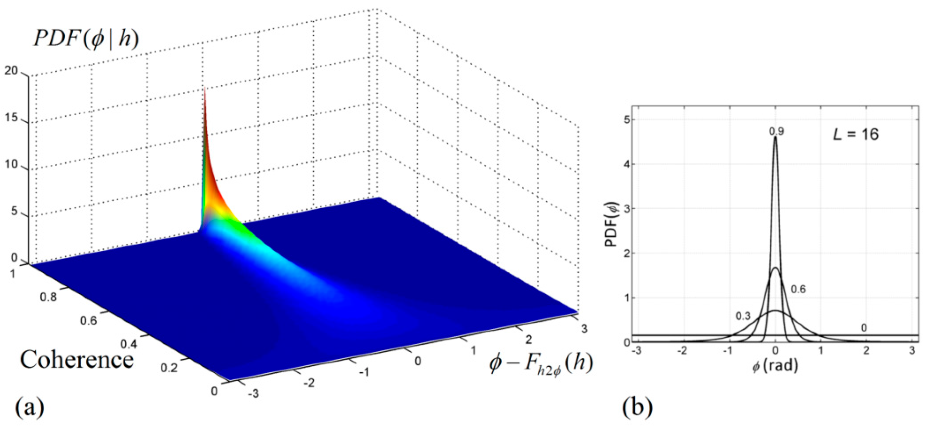
Remotesensing 10 00454 g001
Figure 2. (a) The fitted surface by the look-up table with ENL L = 16 and (b) the profile perpendicular to the coherence axis with ρ = 0.3 , 0.6 , 0.9 .
Remotesensing 10 00454 g002
Figure 3. (a) Hillshade of 10 m NED DEM; (b) hillshade of 15 × 15 smoothing filtered NED DEM; (c) NED DEM (upper) and smoothing filtered NED DEM (lower); (df) are the simulated interferograms I, II, and III, respectively, and the phase noise introduced by decorrelation is superimposed; (gi) are the simulated atmospheric phase for interferograms I, II, and III, respectively; (jl) are the simulated interferograms I, II, and III superimposed by the atmospheric phase (gi), respectively.
Remotesensing 10 00454 g003
Figure 4. Multi-baseline InSAR DEMs (without atmospheric effects) and height error maps, without the prior DEM (a,b) and with the prior DEM (ce) is the hillshade of (c) with the enlarged topographic details of a small area.
Remotesensing 10 00454 g004
Figure 5. (a) Multi-baseline InSAR DEM with prior DEM (with atmospheric effects); (b) height error map; (c) is the hillshade map of (a).
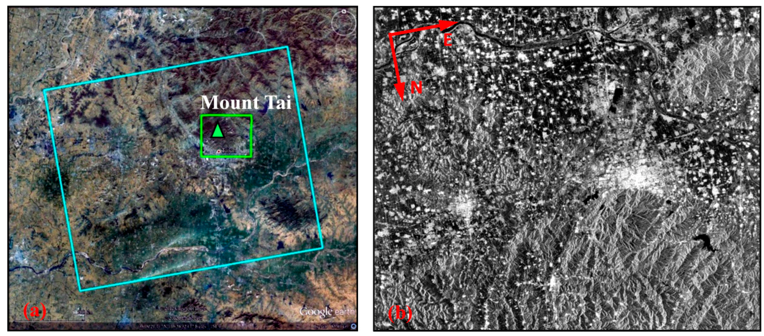
Remotesensing 10 00454 g005
Figure 6. (a) The coverage of ALOS/PALSAR images marked by the blue rectangle and 1:25,000 DEM marked by the green rectangle shown in Google Earth; (b) the amplitude image of ALOS/PALSAR data (acquisition time: 6 February 2008).
Remotesensing 10 00454 g006
Figure 7. The temporal and spatial baseline distribution of ALOS/PALSAR interferometric pairs. The images connected by the blue line constitute interferometric pairs and the interferograms connected by the red line are co-registered to the same image space.
Remotesensing 10 00454 g007
Figure 8. Flattened interferograms of the ALOS/PALSAR data. (a) Interferogram I, B = 784 m; (b) Interferogram II, B = 77 m; (c) Interferogram III, B = 561 m; (d) Interferogram IV, B = 185 m.
Remotesensing 10 00454 g008
Figure 9. Hillshades of single/multi-baseline DEMs and SRTM DEM corresponding to the black rectangle in Figure 8a. (a) Multi-baseline InSAR DEM; (b) radar-coded SRTM DEM; (c) Interferogram I DEM, h 2 π = 82 m; (d) Interferogram II DEM, h 2 π = 833 m; (e) Interferogram III DEM, h 2 π = 115 m; (f) Interferogram IV DEM, h 2 π = 347 m.
Remotesensing 10 00454 g009
Figure 10. Hillshade of multi-baseline InSAR DEM. The black rectangle marks the coverage of the 1:25,000 DEM used for accuracy validation.
Remotesensing 10 00454 g010
Figure 11. The height error map of InSAR DEMs, (a) the DEM generated by ML estimation with prior DEM; (b) SRTM DEM; (cf) are the DEMs generated by single-baseline interferograms I, II, III, and IV.
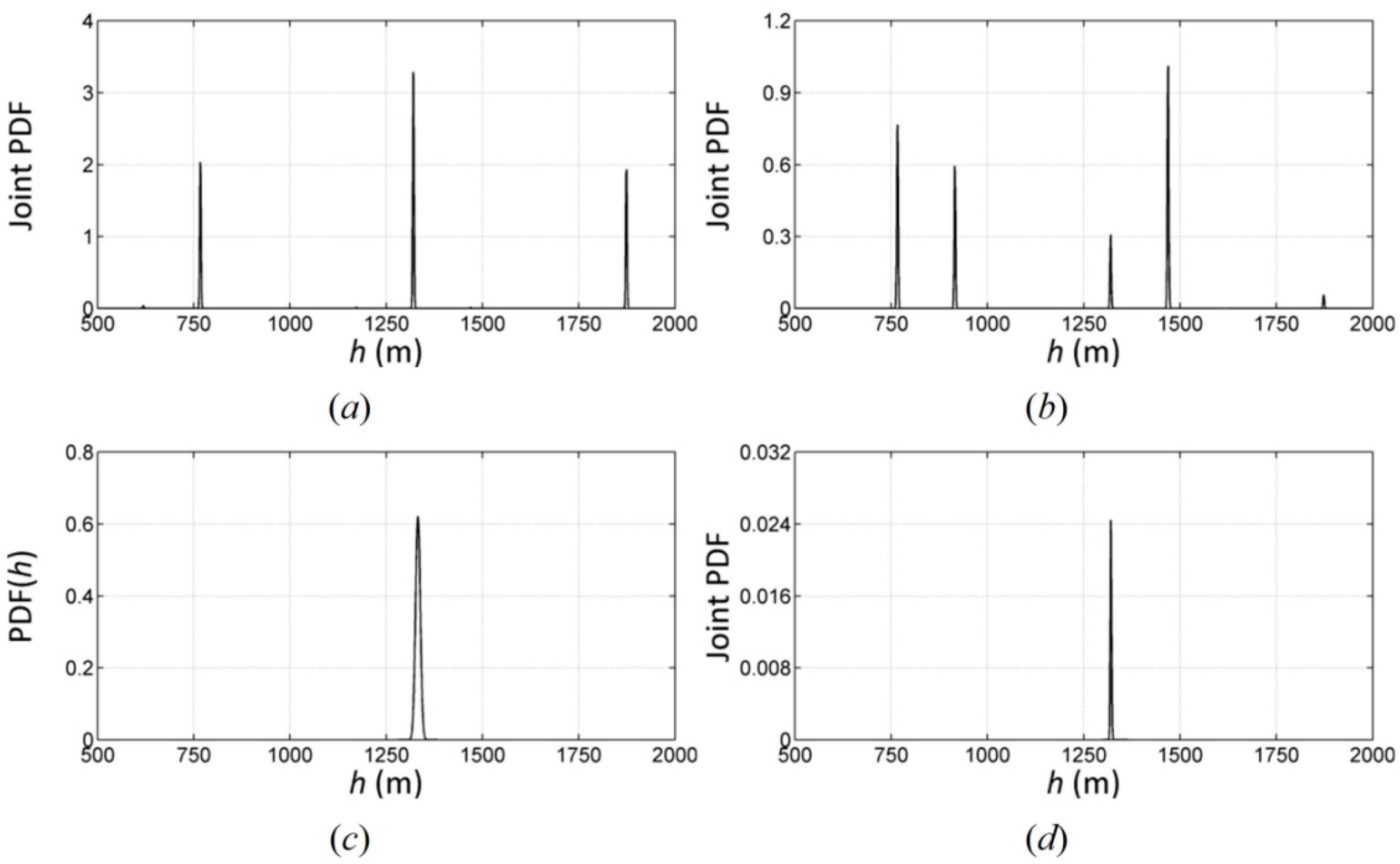
Remotesensing 10 00454 g011
Figure 12. The height probability distribution of a cell in the simulated interferogram with a true height of h = 1320.4 m. (a,b) The joint height probability distribution with and without decorrelation phase noise, respectively; (c) the prior height probability distribution acquired from the prior DEM; (d) the joint height probability distribution with the prior height probability distribution, obtained by multiplying the two probability distributions in (b,c).
Remotesensing 10 00454 g012
Table 1. Height-to-phase conversion errors of rational function model.
Spaceborne InSAR DataHeight AmbiguityHeight-To-Phase
Max. ErrorRMSE
ALOS/PALSAR82 m1.97 × 10−3°2.14 × 10⁻⁴°
COSMO-SkyMed164 m−4.08 × 10⁻⁴°6.78 × 10⁻⁵°
TerraSAR-X59 m−1.81 × 10⁻³°2.15 × 10⁻⁴°
Table 2. The simulation parameters of the interferograms.
Interferogram IInterferogram IIInterferogram III
Normal baseline47 m83 m178 m
Height ambiguity139.54 m79.02 m36.84 m
Coherence coefficient0.600.570.51
Std. of phase noise0.254 rad0.277 rad0.333 rad
Table 3. Statistical values of height errors without atmospheric effects.
MeanStd.
Prior DEM0.007 m4.7 m
Interferogram I (Figure 3d)0.002 m5.6 m
Interferogram II (Figure 3e)−0.010 m3.5 m
Interferogram III (Figure 3f)−0.001 m2.0 m
ML without prior DEM70.072 m408.8 m
ML with prior DEM−0.003 m1.6 m
Table 4. Statistical values of height errors with atmospheric effects.
MeanStd.
Interferogram I (Figure 3j)−2.5 m16.2 m
Interferogram II (Figure 3k)2.5 m8.7 m
Interferogram III (Figure 3l)−0.6 m4.6 m
ML with prior DEM−0.006 m4.1 m
Table 5. Image parameters for ALOS/PLASAR data.
Acquisition Time22 December 2007/6 February 2008/23 March 2008/
27 December 2009/11 February 2010/29 March 2010
Orbit directionAscending
Imaging modeStripmap
PolarizationHH
Central incidence angle38.7°
Sampling space of azimuth/range direction3.18 m/4.68 m
Band width of azimuth/range direction1522 Hz/28 MHz
Table 6. Parameters for ALOS/PALSAR interferometric pairs.
Interferogram IInterferogram IIInterferogram IIIInterferogram IV
Acquisition time of the Master image6 February 20086 February 200811 February 201011 February 2010
Acquisition time of the Slave image22 December 200723 March 200827 December 200929 March 2010
Temporal baseline46 days46 days46 days46 days
Normal baseline B −784 m77 m−561 m185 m
Height ambiguity h 2 π 82 m833 m115 m347 m
Central Doppler frequency74/75 Hz74/80 Hz68/57 Hz68/46 Hz
Mean coherence coefficient0.520.530.580.50
Table 7. Statistical values of height errors of single/multi-baseline InSAR DEMs and SRTM DEM.
MeanStd.Absolute Value ≤ 10 m
SRTM DEM4.9 m15.4 m58.9%
Interferogram I DEM1.9 m11.3 m81.4%
Interferogram II DEM−4.4 m43.0 m32.8%
Interferogram III DEM2.3 m10.6 m83.0%
Interferogram IV DEM−0.3 m27.7 m51.8%
multi-baseline DEM1.7 m8.6 m86.3%

