1. Introduction
Object detection has been a key factor in high-resolution remote sensing images (HR-RSIs) analysis, and has been extensively studied for the remote sensing community. It is basic but challenging, due to the fact that HR-RSIs contain objects with different textures, shapes, and complex backgrounds and are always affected by different imaging conditions caused by weather, clouds, sun elevation angles, etc.
Due to recent advancement in remote sensing technology, the detection of small moveable manmade objects becomes possible, and the focus of object detection in remote sensing has been gradually moved to relatively small targets, such as vehicles, airplanes, and ships, from large man-made infrastructures such as airports and residual areas. This shift leads to a situation in which, on the one hand, the induced information in HR-RSIs can easily affect the detection accuracy by the background, and on the other hand makes it hard to find frequently partially occluded objects with missing information. This paper exactly concentrates on partially occluded object detection (POOD) in HR-RSIs with high accuracy.
The state-of-the-art object detection methods for HR-RSIs can be roughly categorized into two groups. The first group of methods are based on deep learning (mainly the convolutional neural network (CNN) based methods [
1,
2,
3,
4,
5,
6,
7,
8,
9,
10]), which use a large amount of samples to train a deep layered neural network and learn deep feature representation to classify the candidate regions into objects and background. Its performances on ordinary unoccluded HR-RSI datasets is remarkable and superior. However, state-of-the-art CNN-based methods are unable to precisely handle the occlusion problem. Although some tricks [
11] can be applied to tackle it to some extent, its capability is rather limited. For example, the data augmentation method [
12] is always used to extend the training set to account for different transformations of objects, such as sample cropping. However, the trained network can only detect the unoccluded object area and will be unable to infer the exact location of the partially occluded object, which is considered to be the essential quality for an object detection method. Moreover, its black-box architecture also makes it relatively hard to accommodate heavy occlusion [
13] which is very common in HR-RSIs.
The other group of methods have handcrafted features or handcrafted architectures [
13,
14,
15,
16,
17,
18,
19,
20,
21,
22]. They either concentrate on better feature representation for objects [
18,
19], or focus on flexibly modeling the object structures and appearance [
17,
20], or try to design a better classifier [
21,
22]. This group has been extensively studied in previous decades before the emergence of deep learning-based methods. The deformable part-based method (DPM) proposed by Felzenszwalb [
15] is an outstanding generic object detection method in this group. It models object structure with a pictorial structure model and object appearance with part and root filters. Successively, researchers introduce DPM into object detection in HR-RSIs [
14,
16,
20,
23,
24]. However, researchers demonstrate that the performance of DPM will drop greatly when occlusion happens [
17,
25]. The fact is that the detection tasks in varied applications using HR-RSIs are always accompanied with large occlusion.
To tackle this, Ouyang et.al. and Niknejad et al. [
26,
27] both firstly utilize DPM to detect the scores of parts and then infer the occlusion with a hierarchical deep belief network and a two-layer conditional random field. These two methods concentrate on the inference of occlusion based on the scores of parts at hand. Different to these, our previous work [
17] proposed a two-layer object model named partial configuration object model (PCM) to deal with the occlusion problem in HR-RSIs. It designs several partial configurations to detect the unoccluded evidences and finally synthesizes these evidences to justify the presence of an object. Its idea is very simple and the result is promising. However, it requires a great amount of manual predefinition and massive computation [
13]. To solve the problem of PCM, an automatic and fast PCM generation method, AFI-PCM, was proposed by us in [
13]. It proposed a part sharing mechanism to tackle the above problem, thereby making the automatic implementation of PCM possible. However, it only pays attention to the model training stage of PCM and the more concerned detection stage is exactly as slow as PCM.
The work in this paper is inspired from the problems in PCM and AFI-PCM, which tries to integrate the entire PCM model with a novel part sharing mechanism for both fast and automatic model training and detection, that is, a unified PCM framework for fast POOD. To the best of our knowledge, no PCM/AFI-PCM–like POOD methods are reported currently, except for Refs. [
13,
17]. The work in this paper is a largely extended version of our previous work [
13,
17]. The contributions of the work can be found in four aspects: (1) we analyze the shortcomings of PCM and AFI-PCM in detail, and give the inherent causes that lead to these shortcomings; (2) we propose to use a part sharing mechanism for fast POOD, which will get around the PCM assembly process. It makes the entire training and detection processes a unified framework, and obtains great detection speedup compared to PCM and AFI-PCM. Experimental results not only verified the speedup, but also show that it can obtain a comparable accuracy with PCM; (3) we propose a novel spatial interrelationship estimation method directly from the deformation information of DPM model; (4) we propose to simultaneously learn the weights within a partial configuration and the weights between partial configurations in a unified way.
The remainder of this paper is organized as follows.
Section 2 analyzes the shortcomings of PCM and AFI-PCM in detail and gives their inherent causes.
Section 3 gives detailed information about the proposed unified PCM framework for fast POOD.
Section 4 shows the experimental results. And conclusions are drawn in
Section 5.
2. Shortcomings Analysis
In this section, we first briefly introduce PCM and AFI-PCM which are both designed for POOD in HR-RSIs, and then give detailed shortcoming analysis of these two methods. For convenience, we take the airplane category as an example to elaborate all related ideas hereinafter.
2.1. Brief Review of PCM and AFI-PCM
Compared to conventional single-layer object detection methods like DPM, PCM defined an extra buffer layer to block the occlusion impact from passing onto the object layer. This layer is intended to encode possible occlusion states. It is named as partial configurations which is the configuration of adjacent predefined semantic parts. Each partial configuration is represented by a standard DPM model.
The basic unit in PCM is semantic part. They are selected from a predefined category-dependent undirected skeleton graph. The definition of semantic parts determines the coverage of partial configurations. The coverage will then be used to estimate the spatial interrelationship that converts partial configuration hypotheses into full-object ones in the second layer of PCM. The second layer is the object layer that is the arrangements of partial configurations. Instead of the commonly used linear-scoring mechanism, a max-scoring one is used in the object layer to ensure that even certain partial configurations are occluded; the remained partial configurations will still have the chance to capture the unoccluded evidence of the presence of object to finally detect the object. During detection, unoccluded partial configurations will contribute to the locating of the partially occluded objects.
AFI-PCM mainly aims at the training stage for automatic and fast implementation of PCM. Based on the idea that a trained DPM model contains all the elements that PCM needs, AFI-PCM proposes to share part and root filters within partial configurations. It means that AFI-PCM find another way around to directly assemble these elements to generate new PCM models, while still following the detection pipeline of PCM. AFI-PCM adds an extra DPM filter layer into the two-layer object architecture of PCM for training, and uses the same two-layer architecture for model detection.
2.2. Shortcomings of PCM
In this section, we extend the analyses in [
13] about shortcomings of PCM from four perspectives.
2.2.1. Uncertainty of Semantic Parts and the Gap between Semantic Parts and Parts in Detection
The semantic part is the basic element in the first layer, of which the combination determines the coverage of partial configurations. The semantic parts are defined manually and semantically, along with the skeleton graph of the category. Generally, it is hard to determine whether the defined semantic parts are suitable for detection.
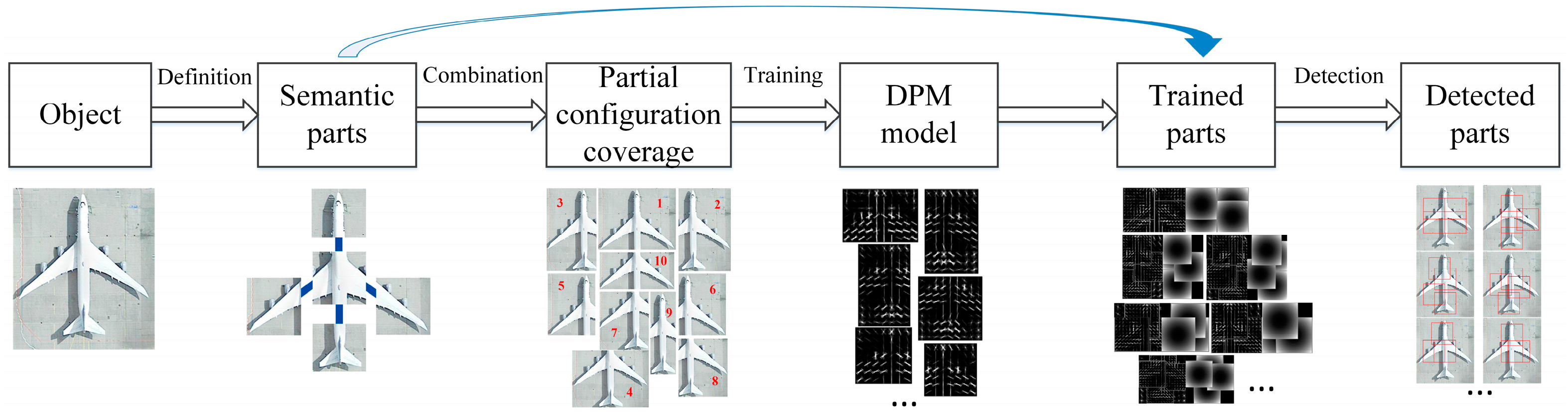
Actually, the semantic parts are not explicitly used in the partial configuration layer. They are only used to calculate the coverage of partial configuration. Partial configuration is represented by a standard DPM with parts located at salient points of the object. Therefore, these semantic parts are not the parts that we use for detection. In this way, the human prior does not contribute to the detection.
Figure 1 shows all related parts in the entire train and detection chain. It can be seen that semantic parts are different from the parts trained in the DPM model. It also indicates that the entire PCM model is designed with redundancy, as large amount of extra work will be needed to transform the defined semantic parts to the trained parts.
2.2.2. Tedious Sample Annotation and Arbitrary Skeleton Graph Predefinition
As revealed above, obtaining the semantic parts becomes a necessary and unavoidable job in PCM. Moreover, we cannot use definite rules to obtain partial configurations’ coverage directly from the bounding box of a full object, in order to avoid the variances of Gaussian functions of a spatial interrelationship being zero and the following weighted continuous clustering being discretized.
For PCM, annotating the semantic parts of each training sample becomes an inevitable route. However, this work is highly labor-intensive. Though it tries to reduce the annotation volume of a full object through semantic part combination, a large amount of additional annotations is still needed, compared to general object detection methods which only need full-object annotations.
In PCM, the semantic parts are organized with a category-dependent skeleton graph, and this graph should be defined beforehand for each category by operators. This predefinition relies too much on the operators’ subjective understanding, and sometimes it is also hard to tell whether the definition is suitable for detection. The predefinition of the skeleton graph greatly hinders the automatic implementation of PCM to other new object categories.
2.2.3. Repeated Training of Shared Semantic Part Areas
PCM uses multiple partial configurations to handle the occlusion impact. All these partial configurations are separately trained using the samples cropped from the same full object samples according to the coverage combined from the same set of semantic parts. This multi-model training process is actually a repeated process of modeling the same set of semantic part areas, as can be observed in
Figure 1. Therefore, the training of PCM is inefficient.
2.2.4. Repeated Detection of Shared Semantic Part Areas
During the detection stage, each DPM model of partial configuration will slide through the entire image to obtain the corresponding responses of part and root filters. Similarly, for an object to be detected, the multi-model detection process will convolve through its shared semantic part areas 10 times if the number of partial configurations is 10. Therefore, the detection process of PCM is also rather time-consuming. As can be imagined, it will be unsuitable for the applications that online detection speed is crucial for, especially when using very large HR-RSIs.
2.3. Shortcomings of AFI-PCM
2.3.1. Repeated Part Detection and Redundant PCM Packing
AFI-PCM in [
13] tries to speed up the training stage of PCM through a part sharing mechanism. It intends to share the same set of parts from a trained DPM model of a full object, and pack the shared part filters into new PCM models. As a consequence, its detection process is exactly the same as with PCM, and it shares the fourth shortcoming of PCM, that is, the more important detection stage is ignored.
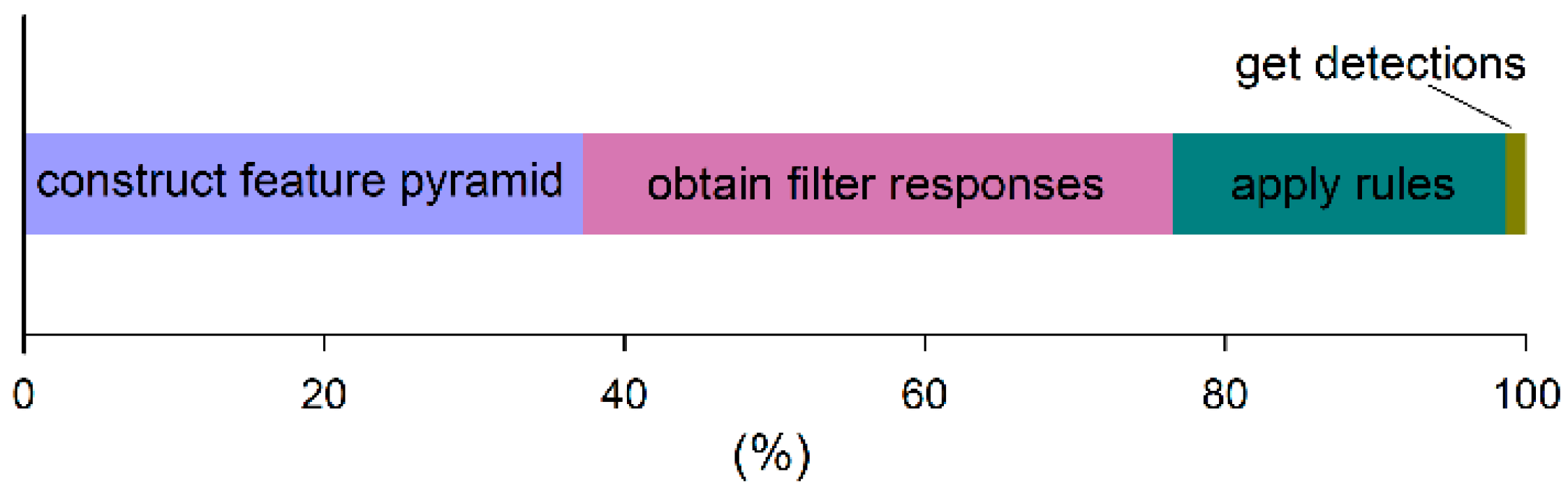
We take a detection example of a partial configuration and
Figure 2 illustrates the detection time consumption percentages of the four main steps: construct feature pyramid, obtain filter response, apply structural rules, and get final detections. The first two steps take more than 75% of the detection computation, while this work is exactly the same for different PCM models for the same image. The remaining two steps are different between different partial configurations but only take less than a quarter of the time. If the first two steps are shared, the computation overhead will be greatly reduced.
2.3.2. Separated Weights Learning among and within Partial Configurations
In AFI-PCM, there are two key factors. One is the weights that balance the performance differences between partial configurations, and the other one is the weights that balance the elements within a partial configuration. In PCM, the former is obtained through a max-margin Support Vector Machine (SVM) optimization method and the latter is done within the DPM method through latent SVM. In AFI-PCM, both parameters are explicitly optimized by the same max-margin SVM optimization method. However, these two optimization processes are separately learnt on two different datasets. Therefore, the optimization error introduced by the first round of optimization will be passed to the second round of optimization and it will be magnified.
2.3.3. Extra Loop in Spatial Interrelationship Estimation
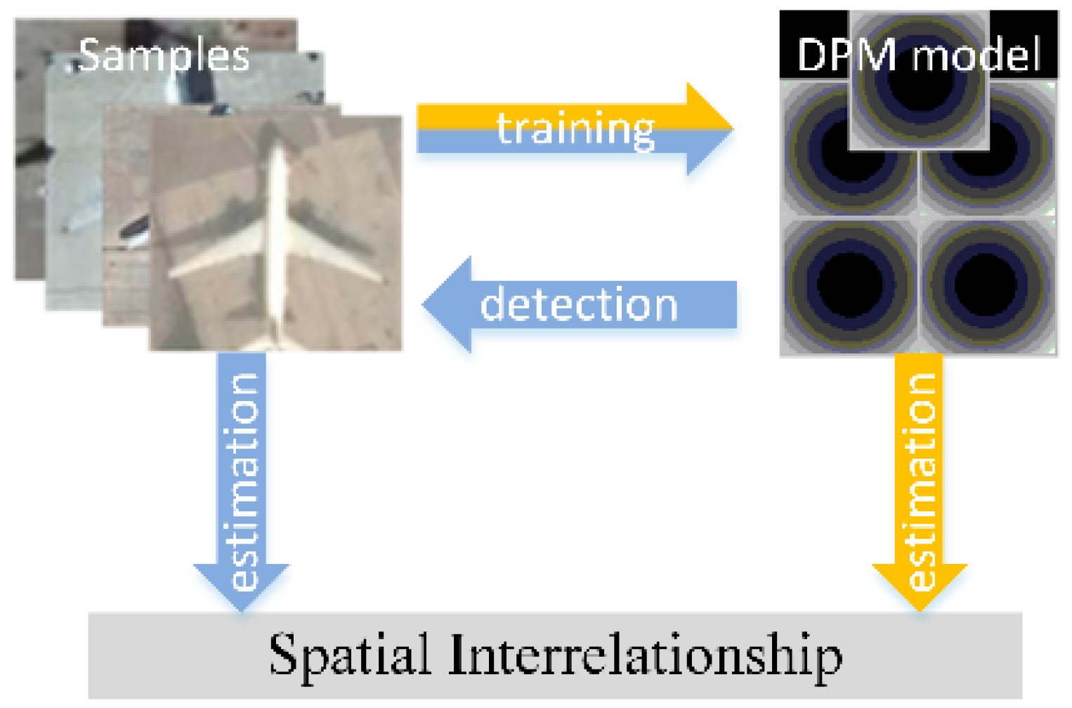
In PCM, the spatial interrelationship is estimated from offsets statistics from the manually annotated partial configuration to the full object. This annotation process is tedious, as analyzed in the above section. In AFI-PCM, this process is made into an automatic one. It uses the trained DPM model to re-detect the training samples to obtain the part locations for spatial interrelationship estimation. However, there is an extra loop in this process (See the blue arrows in
Figure 3), although already better than manual annotation. DPM learns the part deformation from massive training samples, and then it is used to redetect the training samples for part location variations. These variations are finally used to estimate the spatial interrelationship. The evident loop also takes a great amount of time in the training stage.
2.4. What Are the Causes of These Shortcomings in PCM and AFI-PCM?
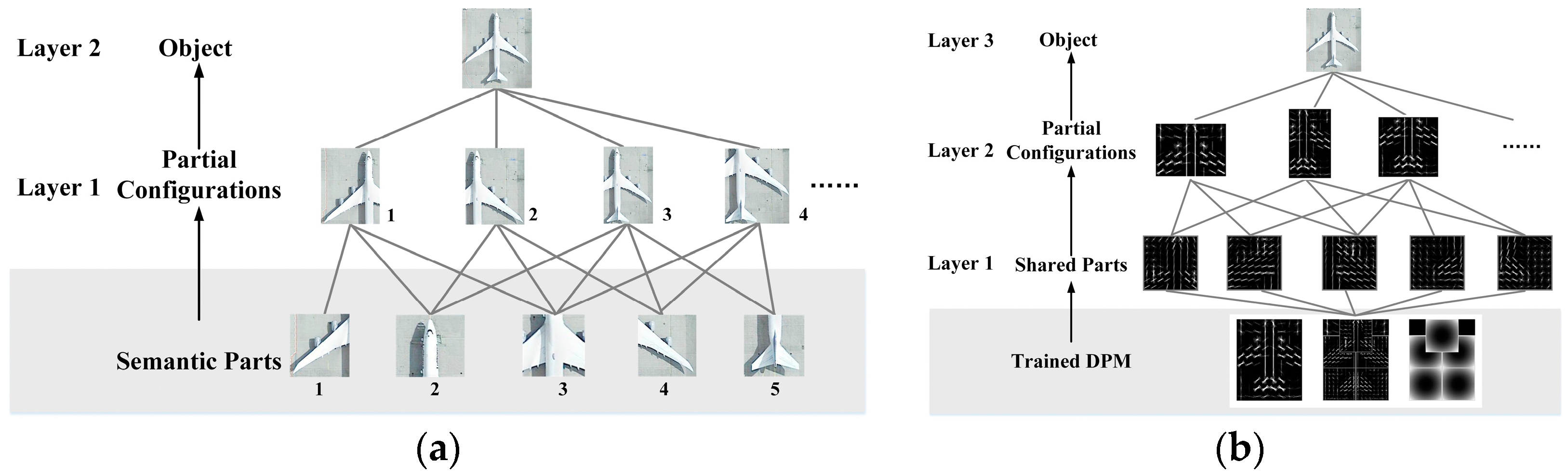
PCM consists of two layers. The first layer is the partial configuration layer, and the second layer is the object layer. There is also a hidden layer in PCM, the semantic part layer, which is the basis of the first layer. The architecture of PCM is given in
Figure 4a. The number of subjects/items in the first layer is much greater than other layers. As revealed above, the main body of all training or detection work is involved in the partial configuration layer, and the semantic part layer is only for the purpose of data preparation. This leads to a situation where a large number of subjects need to be trained or detected for the first layer. Although the elements in the partial configuration layer are based on the same basis layer, they do not share the basis during the training and detection, that is, the entire basis layer is separately trained or detected for each partial configuration. We believe that this is where these shortcomings in PCM come from.
As for AFI-PCM, it has a different architecture from PCM. It uses the part layer as its basis layer, and all other layers are constructed from this. However, this benefit is only used for the training stage, not for the more important detection stage. A more unified framework for both training and detection is preferred, as well as the unified parameter learning of different layers. Another cause is that the potential of the trained DPM is not fully explored. For example, the deformation information of an object is already trained from massive samples, so it does not need to re-detect training samples for this information.
3. Unified PCM Framework for Fast POOD
Given the analysis of the shortcomings of PCM and AFI-PCM and their causes, we propose to “sink” the main body of all training and detection work into its lower layer, as indicated in
Figure 4b. We add an extra shared part layer under the original partial configuration layer. The trained DPM model becomes the hidden layer in our architecture. In PCM, all data preparation work, such as annotations, is included in the hidden layer, and the main body of training and detection lies in the first layer. In the proposed architecture, the intention is similar: the data preparation work is for the hidden layer of training DPM and the main body of training and detection goes to the first layer for shared parts training and detection. We also keep the merits of PCM, which uses fully visible samples to train PCM for partially occluded objects.
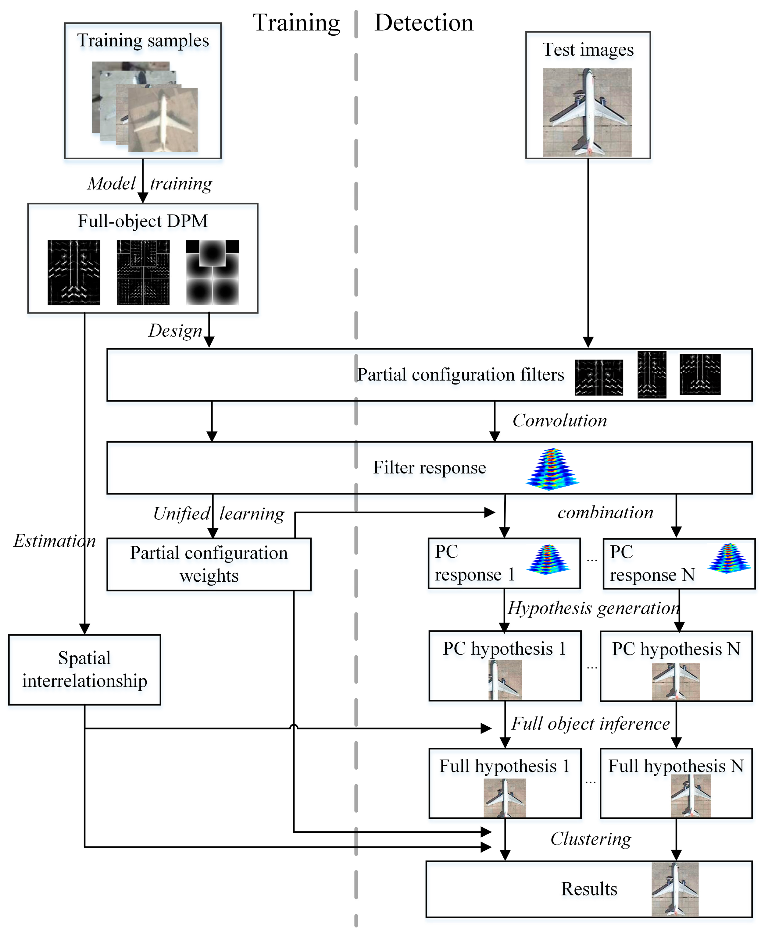
In this section, the proposed unified PCM framework (UniPCM) for fast POOD is described in detail. The proposed framework is illustrated in
Figure 5, which can be divided into several aspects. For the training stage, the original multi-model training process is replaced by (1) single model training; (2) partial configuration design; (3) spatial interrelationship estimation; and (4) unified weights learning. The multi-model detection stage is changed into a single model detection and part sharing based results combination. We firstly give the motivation for a part sharing mechanism, and then describe the key points of the proposed UniPCM framework for fast POOD.
3.1. Part Sharing Mechanism
We first take a look at the first shortcoming of PCM. Once the coverage of partial configuration is set, all related parts are consistent in the following training and detection processes, that is, no gap exists anymore, as can be seen in
Figure 1. Since the parts of DPM cannot be annotated beforehand, PCM uses the semantic parts with similar functions to replace them. This is the cause of the second shortcoming. If we can use the same set of parts for both annotation and training, the gap between the semantic parts and the parts in DPM could be bridged.
Once we obtain a DPM model, the coverage of partial configurations can be determined based on its parts’ locations. Hence, in this paper, we propose to directly use the parts trained from DPM as our semantic parts. Actually, this DPM model is a full-object model trained from fully visible samples. Although the parts of a full object DPM model have no semantic meaning, they do cover certain salient areas of the object. Their combination can also represent occlusion patterns which are most related to POOD using this DPM model. In this way, no skeleton graph has to be defined beforehand since the spatial configuration of parts in DPM is already trained from samples.
For the third shortcoming, the overlapping areas of partial configurations have already been trained, so there is no need to re-train them if we directly use the parts from the trained DPM model. Accordingly, we propose to directly share these part filters for partial configurations. In this way, only one model needs to be trained, which will largely speed up the training process.
The fourth shortcoming of PCM is similar to the third one. In PCM, each partial configuration will detect their own parts. Once the parts are shared, only one set of original parts needs to be detected, and the results of partial configurations can thus be inferred from them, which is the same situation with AFI-PCM.
As revealed above, the part sharing mechanism mainly operates for/at the parts of PCM, and successfully “sinks” the main body of training from the partial configuration layer in PCM (
Figure 4a) to the shared part layer in
Figure 4b. Consequently, part sharing exactly solves the shortcomings mentioned above for PCM and AFI-PCM, and will largely speed up training and detection simultaneously.
3.2. Partial Configuration Design
Different from PCM that uses predefined semantic parts and a skeleton graph to generate partial configurations, all that is available for our method is the trained full-object DPM model. As each partial configuration is represented by a DPM model, we need to prepare the root filter, part filters, and deformation information for a new partial configuration model, which is described in the following subsections.
3.2.1. Part Selection
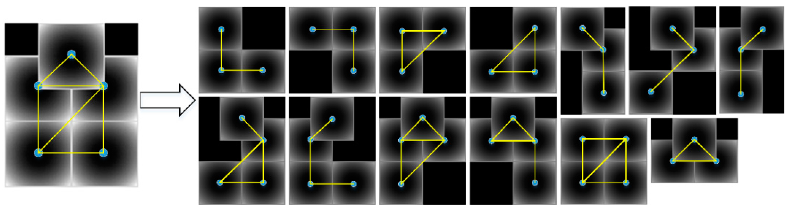
The first thing is to determine which parts to be combined into the new model. Each part in DPM model is characterized by its deformation anchor and size, which is a good guide for our determination. Without the skeleton graph, there are arbitrary possibilities of part combination. There are always many unreasonable combinations, representing the occlusion patterns that are not likely to happen in applications. For the case of remote sensing, geospatial objects on the ground are more likely to be occluded by larger occluders, such as clouds or its functional facilities. The occlusion patterns, such as a hollowed-out occlusion pattern, are unlikely to happen or very rare. In PCM, these unreasonable patterns are filtered out with the aid of a predefined skeleton graph. In our work, the only guide is the parts’ locations. Therefore, we relax the skeleton graph to a more generalized one. We form a net-like graph based on the anchor locations of parts, and then choose all possible sub-graphs from this graph, like PCM under connectivity constraints to leave out unreasonable possible combinations.
For a trained DPM model with
parts represented by
where
corresponds to the part filter parameters,
is its anchor position relative to the root and
is the deformation parameter; the location set
can be formed into a new undirected and connected graph
, see Equation (1) and
Figure 6. It is implemented by the iterative Delaunary triangulation method in [
28].
The main difference between this net-like graph and the skeleton graph in PCM is that the former is generated automatically according to parts’ locations and the latter is defined by human operator. This graph is more consistent with the DPM model for detection, as analyzed in
Section 2.
When the graph is settled down, the partial configuration design process is the same with [
13,
17] which is to select a sub-graph from
while maintaining the connectivity constraint [
29] and the vertex number constraint. These two constraints are used to model the location and ratio of occlusion. An example of this graph is given in
Figure 6. This process can be formulated as automatically choosing a connected sub-graph
from
as Equation (2) and the selected part index set is formulated as
.
When the part index set of each partial configuration is determined, we directly select the corresponding part parameters of from the trained DPM model as the parts of the partial configuration and keep their deformation parameters unchanged.
3.2.2. Root Cropping
The next step is to generate the root filter of partial configuration. The root filter for DPM is a parameter matrix that will convolve through the feature space to obtain the global appearance response of the object. For a partial configuration, its coverage is calculated from the minimal bounding rectangle of its selected parts. Then we directly crop the root filter parameter matrix according to this calculated coverage. The obtained root filter parameter matrix will be reweighted in the following step. Once the new root filter is set, the deformation anchors of parts are shifted to their actual locations.
Up until now, we have completed the work for selecting parts and cropping root from the trained DPM model. The last step away from a complete DPM model is the balance between the selected parts and cropped root.
3.3. Unified Weights Learning
In PCM, partial configurations are unbalanced and need to be weighted. We call this process inter-partial-configuration (inter-PC) weights learning which is conducted on the validation samples using a max-margin SVM framework. Actually, the shared filters in a partial configuration are also unbalanced and need to be reweighed as well. We call this intra-partial-configuration (intra-PC) weights learning. To combine these two processes into the entire framework of PCM, a natural idea is to coarsely aggregate these two reweighing processes. However, intra-PC parameters are intermediate results, and will be implicitly used in inter-PC weights learning. Moreover, they are two separated processes conducted on two different sample sets. The quality of intra-PC weights learning will largely affect the followed inter-PC weights learning.
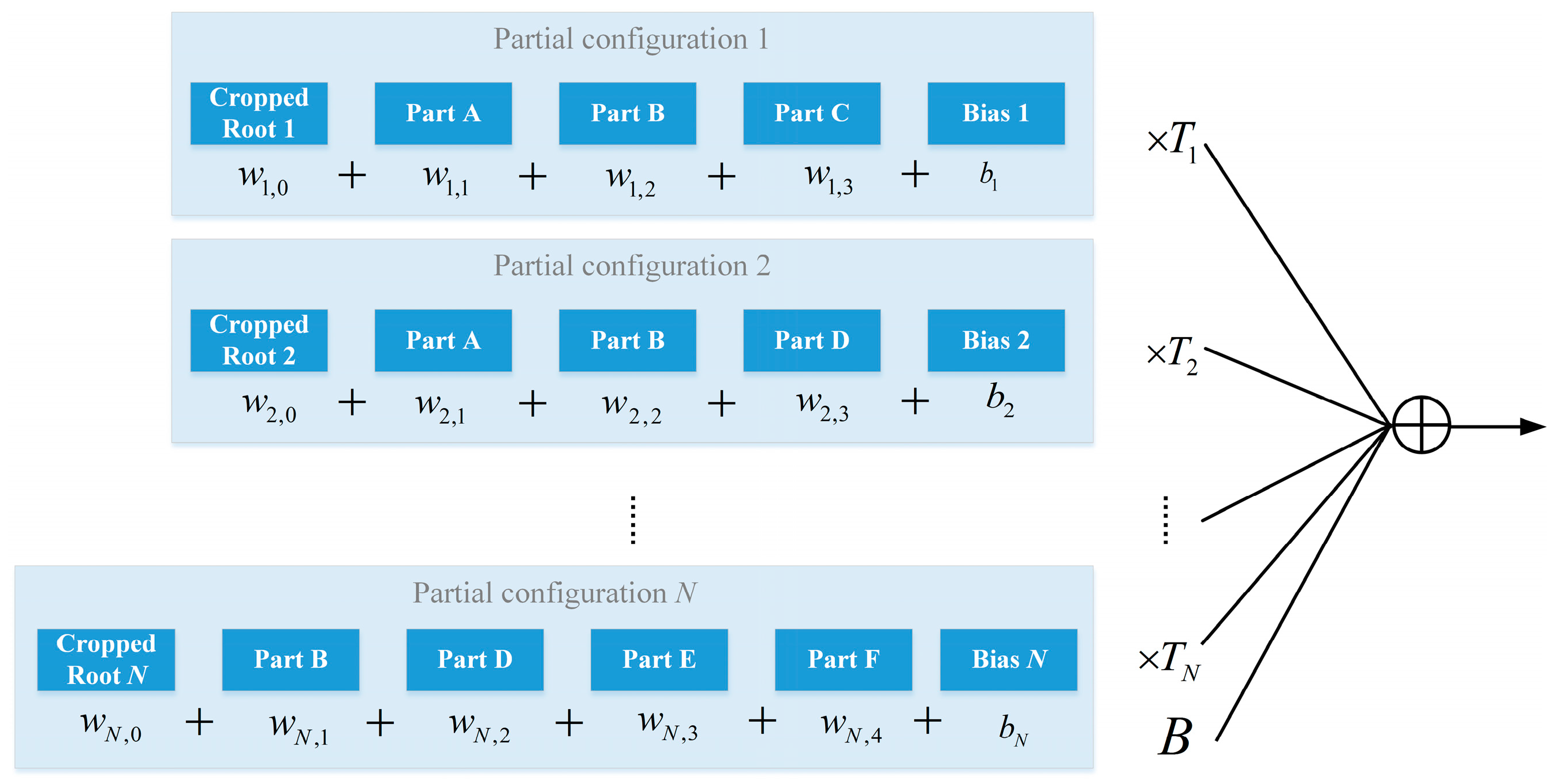
We first review the weights learning process of PCM as illustrated in
Figure 7. In each partial configuration, each component will be assigned a weight
, including a bias term
. When the
partial configurations have settled down, each partial configuration will be assigned a weight
to indicate its importance during the following hypotheses fusion process. In inter-PC weights learning, these scores of partial configurations will be combined with a linear formula. One simple idea is to directly optimize these two processes in one step. However, when the weights are multiplied for inter-PC optimization, it becomes a non-convex problem which is hard to optimize.
To tackle this problem, we propose a unified weights learning framework in this paper, which takes another way around. To separate the multiplied weights for a convex problem, we change the second optimization into a filter reweighing problem, that is, optimizing the weights of all cropped root filters and all part filters, and then obtaining the weights of partial configurations from these learnt filter weights.
For each partial configuration, we optimize the weights of its elements. Let
denotes the score of filter
of partial configuration
i, the score of the partial configuration can be formulated as
The optimization objective function is that the weights make the combination way in Equation (3) match their labels on validation samples. For all prepared filters from the trained DPM model, their score combination should also match their labels
. Let
denote the score of
-th filter (including part filters and cropped root filters), their final label can be formulated as
where
is the weights of two kinds of filters, and
is the bias term. We combine the above two optimization processes into one optimization process that simultaneously obtains the intra-PC and inter-PC weights which are learnt by minimizing the structured prediction objective function:
This standard convex optimization problem can be solved by Lagrange multipliers method using the standard off-the-shelf convex optimization package CVX [
30]. The constants
can be found using 5-fold cross validation.
The relationship between these weights can be formulated as
where
. Once we obtain the above weights
, the inter-PC weights
can be calculated from a least-square solution.
3.4. Spatial Interrelationship Estimation
Through samples re-detection, the partial configuration location distribution can be estimated from the relative offsets of detected parts in AFI-PCM, which is of low efficiency as analyzed in
Section 2. These offset variances actually come from the deformation ability embedded in the DPM model as a match cost like a spring. These deformation parameters are trained from massive training samples, and it is a repetitive process to re-detect the deformation related variances. Based on this fact, we propose to derive the spatial interrelationship directly from the deformation parameters trained in DPM for partial configurations (indicated as yellow arrows in
Figure 3). Its main idea is described as follows.
Given the index set
of a partial configuration, we use their corresponding parts
to derive the location interrelationship and size interrelationship. The deformation cost in DPM for location
is defined as
This deformation cost performs like a spring, and the closer the part locates to the ideal anchor position, the lower the cost will be. This inspires us to transform the deformation cost into a location distribution term. We use a simple conversion function in Equation (8) where
is the anchor position,
is the current position, and
is the deformation parameter vector.
is a normalization function that constrains the data in the range of part size and convert the value range to [0, 1]. Based on the above function, the part location becomes a continuous spatial probability density function (PDF). As can be seen in Equation (7), the deformation cost in DPM is dimension-independent, so the following derivation process can be conducted independently in
and
dimensions.
The location interrelationship represents the relative shift from the center of partial configuration to the object center, and the size interrelationship represents the size ratio between partial configuration and the full object. Given the index set
of a partial configuration and its
, the interrelationships can be estimated as
In Equation (9),
and
represent the right, left, bottom, and top of the bounding boxes of full object and partial configuration. In this way, the continuous interrelationship estimation can be solved as the derivation from the PDFs of parts to the PDF of
based on Equation (9). Fortunately, most of the operations are linear, and they can be directly solved with cascaded operations of PDF estimations. All related formulations of the operations are given in
Appendix A.
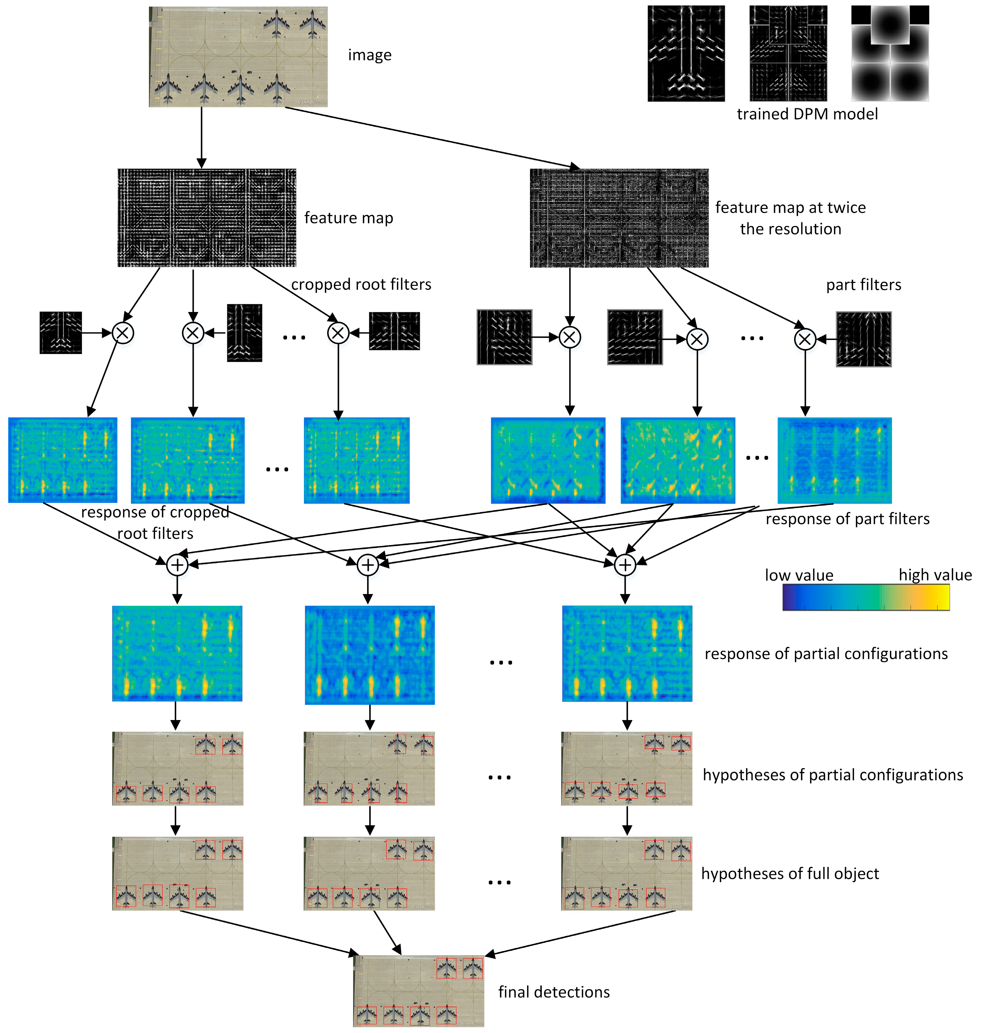
3.5. Unified Detection Framework
In PCM, the obtained models of partial configurations individually slide through the entire image to obtain their corresponding detection results, which means that the computational cost is nearly times as much as that of a full-object DPM model. This paper aims to cut down the computation in both the training and detection stage. Along with the training scheme, our detection is also based on the part sharing mechanism in a unified detection framework, which will largely reduce the computational overhead.
Similar to the training of PCM in that only one DPM model needs to be trained, our detection also needs only one DPM detection with similar computational cost, thereby largely reducing the cost, compared to PCM and AFI-PCM. It means that only one DPM will slide through the image pyramid, and all the POOD work is done based on the results of this DPM.
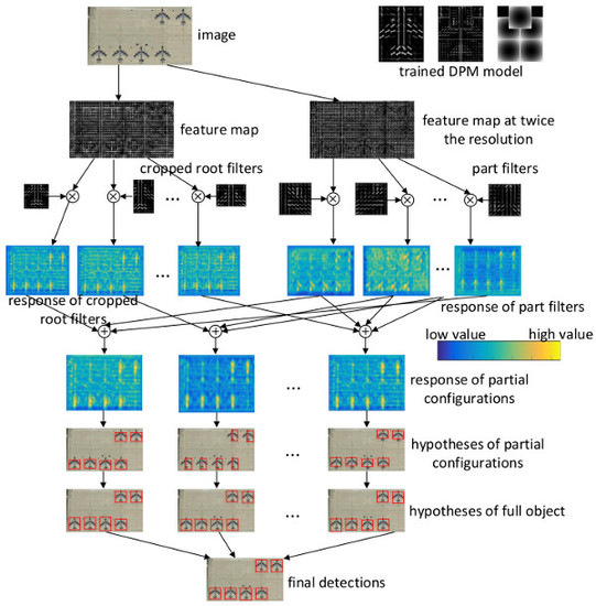
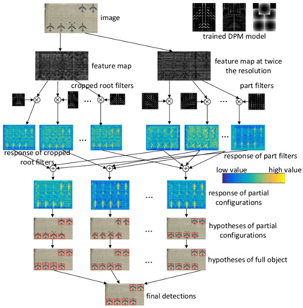
For a trained DPM with parts, we can obtain partial configurations. Therefore, cropped root filters and part filters are prepared for detection from the trained DPM model, along with their weights. In the proposed method, we only have to get the responses of filters and then all responses of partial configurations are obtained.
During detection, we first obtain the responses of all part filters and cropped root filters in the feature pyramid, before they are fed with the trained weights. The weighed responses of the root and part filters of specific partial configuration are combined to yield a final score pyramid for each PC. Different from training, we will then only use the weights of partial configuration to reweigh the responses of PC, rather than forming new results for PCs. Finally the bounding boxes of partial configurations, together with their scores, are predicted as in [
15].
These partial configuration hypotheses will be pre-filtered by a Non-Maximum Suppression (NMS) to ensure that there is only one type of partial configuration in the local area. The following clustering method is the same as PCM. These hypotheses are firstly grouped. In each group, the hypotheses are converted to full-object hypotheses using the spatial interrelationship estimated in
Section 3, which is followed by a weighted continuous NMS method of PCM to obtain the final object bounding box hypotheses.
The entire detection process at one scale is illustrated in
Figure 8.
4. Experimental Results and Discussion
In this section, we provide experimental results and analysis of the proposed UniPCM framework on HR-RSIs. The method is verified on the categories of airplane and ship.
4.1. Data Set Description
For fair comparison with PCM and AFI-PCM, we adopt the same training, validation and test data sets. Their detailed information is provided as follows.
For airplanes, two test sets are used. The first one is the fully visible NWPU10 VHR dataset [
20], with a ground sampling distance (GSD) of 0.5–2 m. Its airplane class is chosen, which contains 89 images with 753 airplanes. The other is the more challenging Occlusion dataset [
17] which is collected from Google Earth service. There are 47 images with 184 airplanes, with GSD ranging from 0.3–0.6 m. Many airplanes in this dataset are occluded by cloud or hangar, or truncated by image border. The training and validation datasets are collected from the similar area with similar GSD. There are, in total, 2810 samples for training and 282 samples for validation. To be noted, no occluded samples are used for training in our framework.
For ships, one occlusion dataset [
17] (hereinafter cited as Ship dataset) is used which is also collected from Google Earth service with a GSD of 0.5–2.4 m. There are, in total, 30 images with 227 ships, 22 objects of which are occluded. The training dataset contains 231 positive samples and 2422 negative samples, and the validation dataset includes 134 samples collected from similar areas.
4.2. Experimental Setup and Evaluation Criteria
To account for in-plane rotation of objects, we manually spilt the full direction into 16 bins, that is, 16 models are used for full-direction detection. The north direction is set as 0. To deal with possible object truncation, we zero-pad the images with 200 pixels for airplanes and 100 pixels for ships. The scale problem of detection is tackled by the inherent multi-scale capacity of DPM through feature pyramid matching. There are 5 parts for both the original DPM models of airplanes and ships. The Intersection-over-Union (IoU) parameter of NMS is 0.3, as calculated in Equation (10). The experiments are conducted on Ubuntu 14.04 LTS with a 4 GHz CPU, a 32 GB RAM, and a NVIDIA Titan X GPU. All codes are implemented with MATLAB.
The detection results are evaluated according to the criteria of [
31]. True positive (TP) refers to a result maintaining an IoU with the ground truth exceeding 0.6, otherwise it is referred as false positive (FP). The unfound ground truths are false negatives (FNs) and the rests are true negatives (TNs). The detection Precision and Recall are defined as
The precision-recall curve (PRC) is used to plot the tradeoff between recall and precision. Average precision (AP) is defined as the area under PRC. Higher AP indicates better performance, and vice versa. As different thresholds yield different precisions and recalls, we use another index,
score, to find the optimal threshold for final detection results. The highest
score makes the best tradeoff between recall and precision, as calculated in Equation (12). A higher optimal
generally means better performance.
4.3. Detection Results
In this section, we evaluate the performance of the proposed UniPCM detection framework on the three test sets. PCM [
17], AFI-PCM [
13], and DPM [
15,
32] are taken as our comparison baselines. Their parameters are chosen according to optimal trails. The DPM model trained for baseline [
15,
32] is then used as for partial configuration design for AFI-PCM and UniPCM. Additionally, a deep learning based object detection method, MSCNN [
33], is also used in our experiments as another baseline. MSCNN is a multi-scale version of the famous Faster RCNN [
34] detection method, which uses feature maps from multiple convolutional layers to enhance the multi-scale detection capability of CNN. Therefore, MSCNN is very suitable for object detection in HR-RSIs. It is originally trained on the much larger dataset ImageNet [
35], and then fine-tuned on our training datasets.
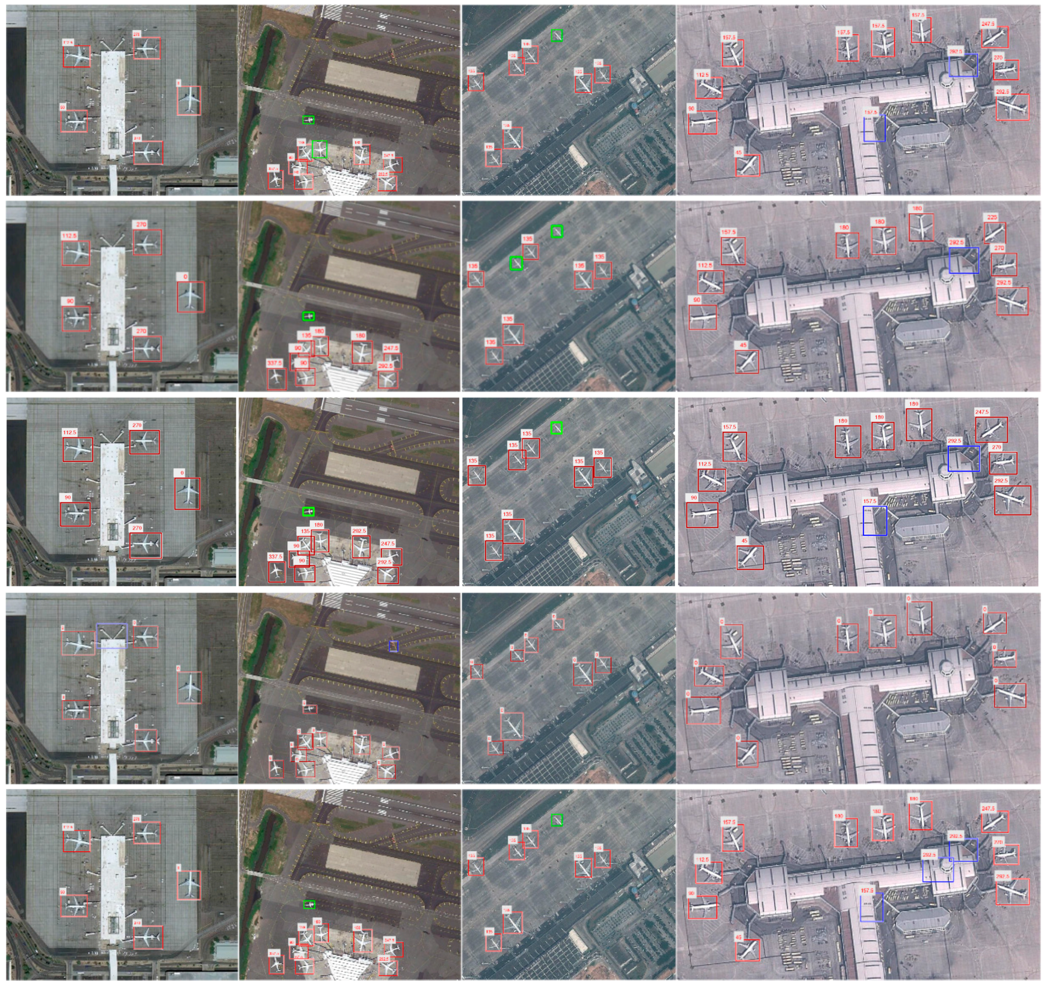
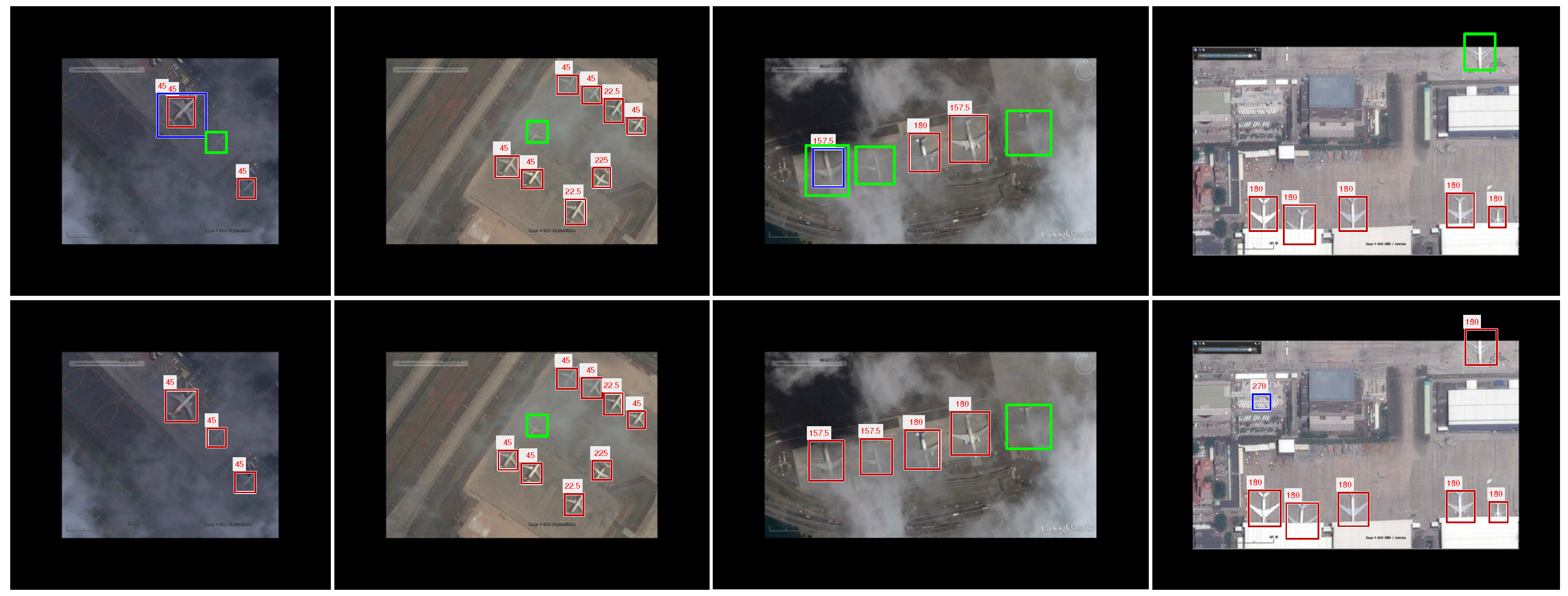
All qualitative detection results are obtained with the threshold that leads to the optimal value. In the following figures, red rectangles correspond to TPs, blue ones correspond to FPs and green ones are FNs. The predicted object direction is denoted above the rectangles. As MSCNN is unable to be direction-invariant, its results are all marked as 0.
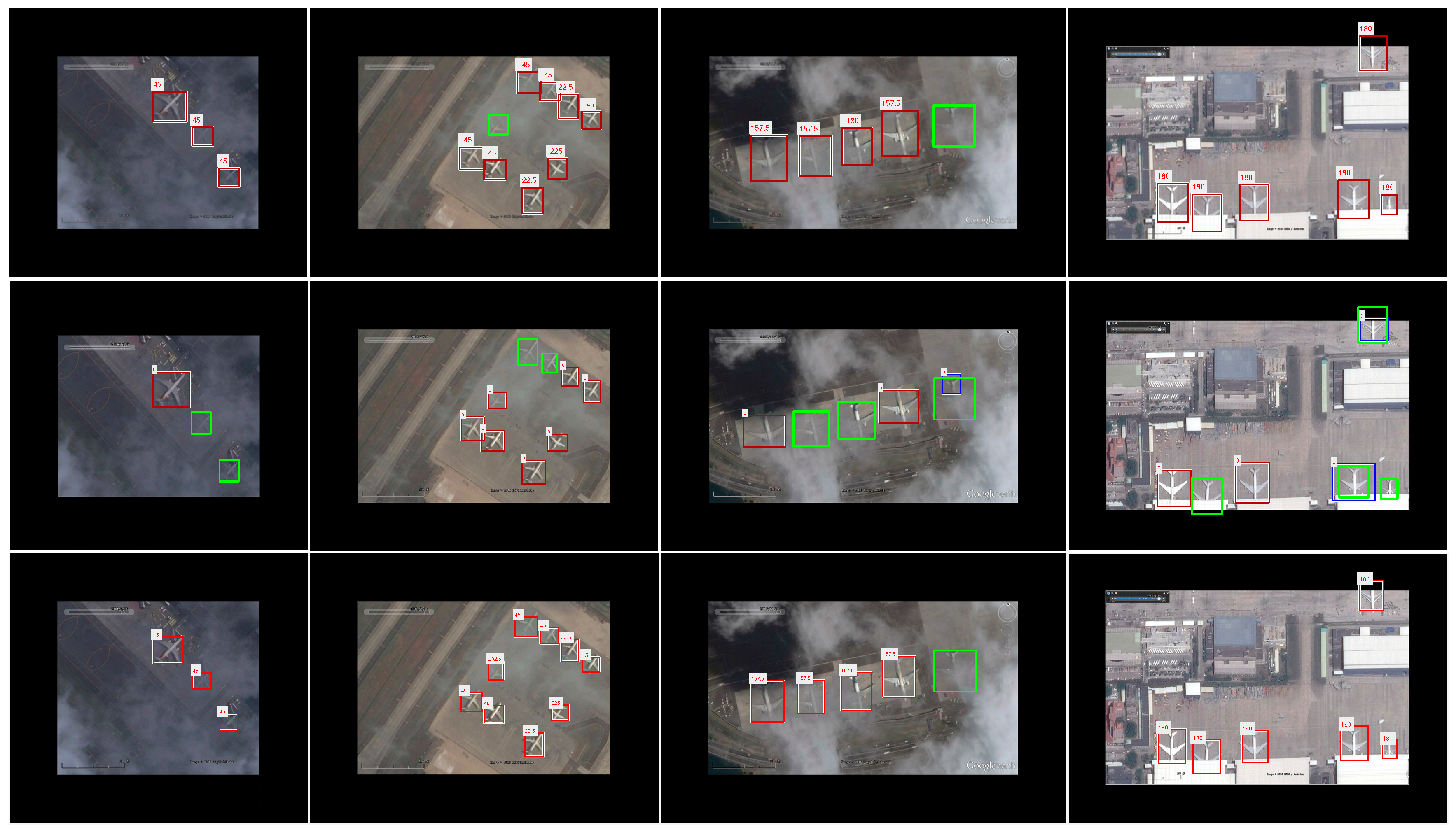
4.3.1. Detection Results on NWPU10 VHR Dataset
We first verify the proposed UniPCM method on the fully visible NWPU10 VHR dataset.
Figure 9 gives some qualitative detection results of all methods. As seen, most of the airplanes are successfully detected by our method, though with some FPs and FNs. The FNs mainly come from the small objects that are also missed by its counterparts, which indicates that it is due to the inherent defects of the trained DPM model. In some images, UniPCM detects some FPs that are avoided by its baselines. As observed, the structures and appearances of these FPs are very similar to that of an airplane as indicated from the predicted object angle, for example the FP in the fourth column. MSCNN obtains the best results among all methods as expected.
The quantitative results of PRC and optimal
values are given in
Figure 10a and
Table 1, respectively. The AP values are denoted in the legend of PRC, which are consistent with the performance difference indicated by optimal
values. It can be observed that UniPCM performs equally to that of PCM and AFI-PCM with very subtle improvement, while outperforming DPM by a large margin. As expected, the deep learning based method, MSCNN, performs best among the methods with an AP up to 0.95. Many airplanes with very small coverage are also successfully detected.
4.3.2. Detection Results on Occlusion Dataset
Figure 11 shows the detection results on the more challenging Occlusion dataset. Despite the fact that partial evidences of objects are missing, the PCM based methods successfully find most of the partial occluded airplanes. UniPCM and AFI-PCM both obtain a few more FNs and FPs, compared to the original PCM. Similarly, some FPs of PCM are avoided by UniPCM and AFI-PCM. Unsurprisingly, the performance of MSCNN decreases greatly compared with that on the NWPU10 VHR dataset. Its capability of discovering partial occluded objects is weak as they are regarded as background with insufficient full-object evidence.
Their performances are also reflected in their PRC and
values in
Figure 10b. The APs and
of UniPCM and AFI-PCM are very close and slightly worse than PCM, but outperform MSCNN and DPM by a large margin. Notably, the early decline of AFI-PCM in PRC does not appear in UniPCM, which indicates that its weights are more reasonable.
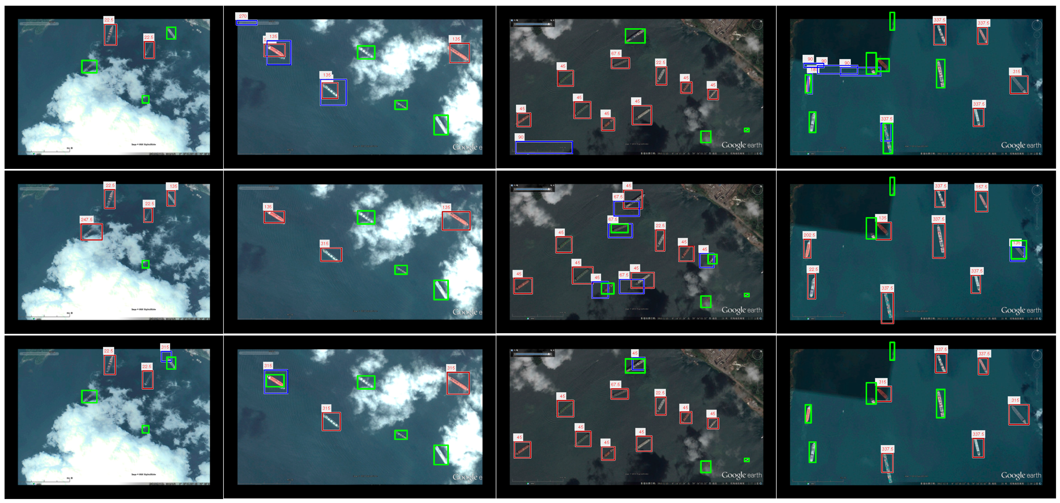
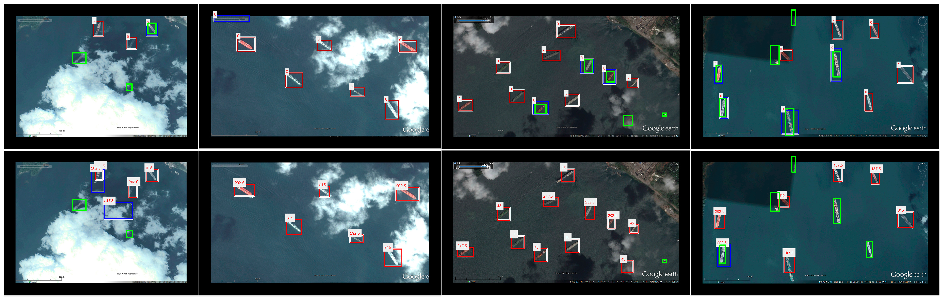
4.3.3. Detection Results on Ship Dataset
As ships vary from length and size, and many of them are in harbors, ship detection has always been a very difficult task [
36]. The detection results on the Ship dataset of all methods are given in
Figure 12. As can be seen, all of the methods obtain a number of FNs and FPs, including the deep learning method MSCNN. Despite the fact that their performances are relatively worse than the airplane datasets, many occluded objects are successfully detected. The ship occluded by cloud in the second column missed by DPM, PCM, and AFI-PCM is grasped by MSCNN and UniPCM. However, MSCNN detects more visible ships and maintains a relatively worse object localization accuracy.
Their quantitative results PRC and optimal
values are given in
Figure 10c and
Table 1. UniPCM achieves the highest AP value among all baselines, which is nearly 0.03 and 0.06 larger than AFI-PCM and PCM. UniPCM obtains the best precision when recall is about 0.15 to 0.4. It partially proves that its scoring mechanism is better than other PCM based methods. Optimal
value is coincident with PRC. AFI-PCM maintains a relatively higher
than UniPCM, while PCM performs worse than these two.
4.4. Scheme Analysis
In this section, we analyze the detection performance of the proposed UniPCM framework under different scheme conditions on the NWPU10 VHR dataset and the Occlusion dataset. The following two factors that will influence the final results are analyzed.
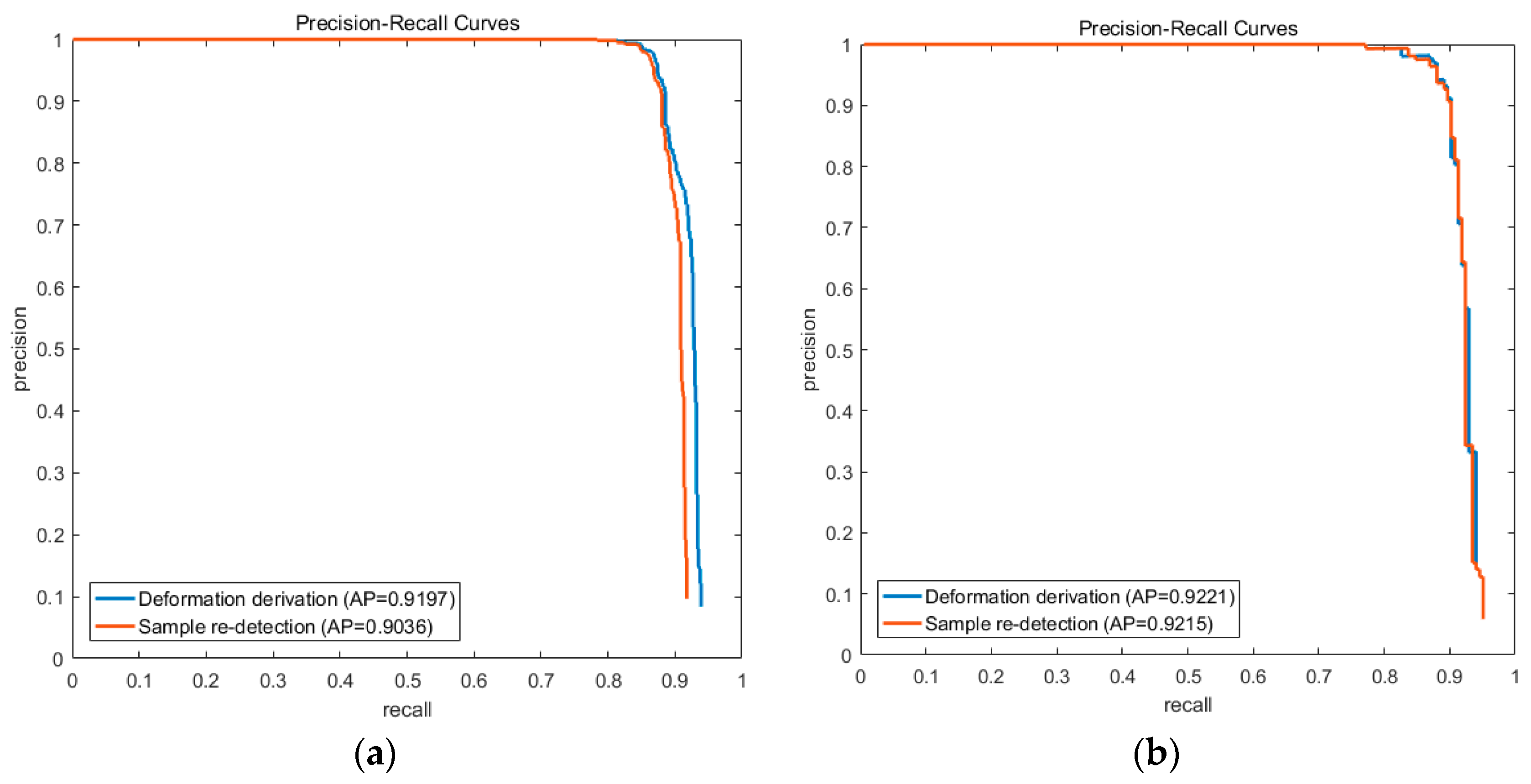
4.4.1. Different Spatial Interrelationship Estimation Schemes
In this paper, we propose to directly estimate the spatial interrelationship from the deformation information of the trained DPM. In AFI-PCM, this relationship is estimated from the re-detection of training samples. We evaluate these two different schemes in our experiments. Their PRC results are illustrated in
Figure 13 with the same experimental configuration.
As illustrated, their performances on the Occlusion dataset are very close to each other, and the deformation derivation scheme is a little better than sample re-detection on the NWPU10 VHR dataset. It is mainly because the sample re-detection process maintains uncertainty during detection, since the part detection is a process of global optimization of all possible locations and it can be affected by varied samples. The results indicate that the deformation derived spatial interrelationship can achieve a slightly better performance with much less computation during estimation.
4.4.2. Different Weights Learning Schemes
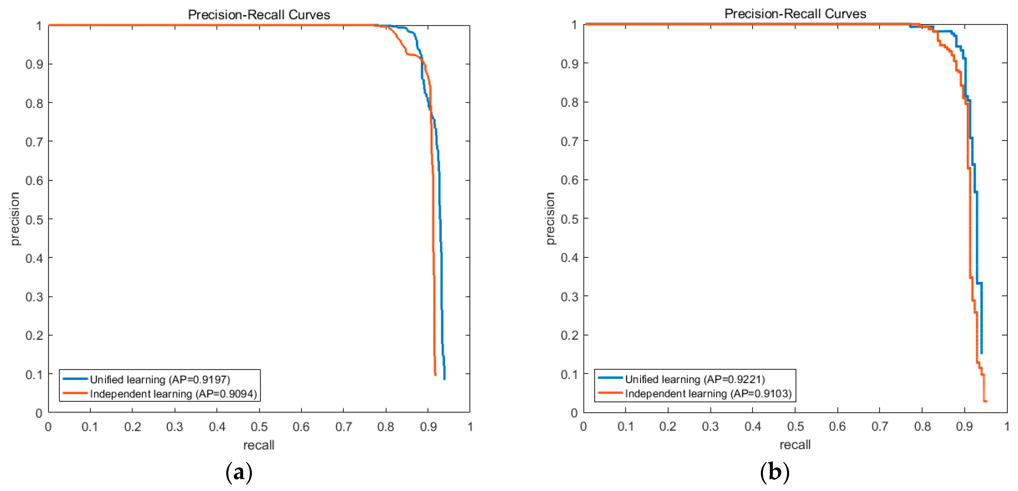
AFI-PCM uses two different datasets to learn independent intra-PC and inter-PC weights, while UniPCM integrates them into one step on only one dataset. To evaluate this difference, we conduct experiments on the independent weights learning scheme and compare them with the results of UniPCM.
Figure 14 shows their PRC results.
Both results on the NWPU10 VHR dataset and the Occlusion dataset illustrate that the unified weights learning process is better than the independent one. On the NWPU10 VHR dataset, UniPCM gets an AP improvement of 0.01 which gets to 0.012 on the Occlusion dataset. It is noticeable that independent learning gets a relatively higher precision when recall is about 0.9, but soon declines dramatically when recall goes up. The results on two datasets verify that unified weights learning can achieve better balance between the elements in partial configurations and also between partial configurations, and is thus better for unified detection than independent learning.
4.5. Training Time Analysis
In this section, we analyze the training time consumed by all baselines. As the architecture of MSCNN is totally different from others, we only analyze the training overhead of DPM, PCM, AFI-PCM, and UniPCM in detail. MSCNN runs on the GPU and takes about 4.5 h for training.
There are two groups of work for PCM training for all these methods. The first one is the manual work that mainly includes sample annotation and category predefinition. For PCM, it contains semantic part definition, category skeleton graph definition, and part-level sample annotation. For AFI-PCM and UniPCM, they only include object-level sample annotation. As manual work is hard to evaluate quantitatively, we do not analyze it in this section. As for manual work, UniPCM and AFI-PCM have already greatly reduced the workload. The annotation work of UniPCM and AFI-PCM is the same with DPM.
The other work for PCM training is the model training. To be brief, we list all related training stages of these three methods in
Table 2.
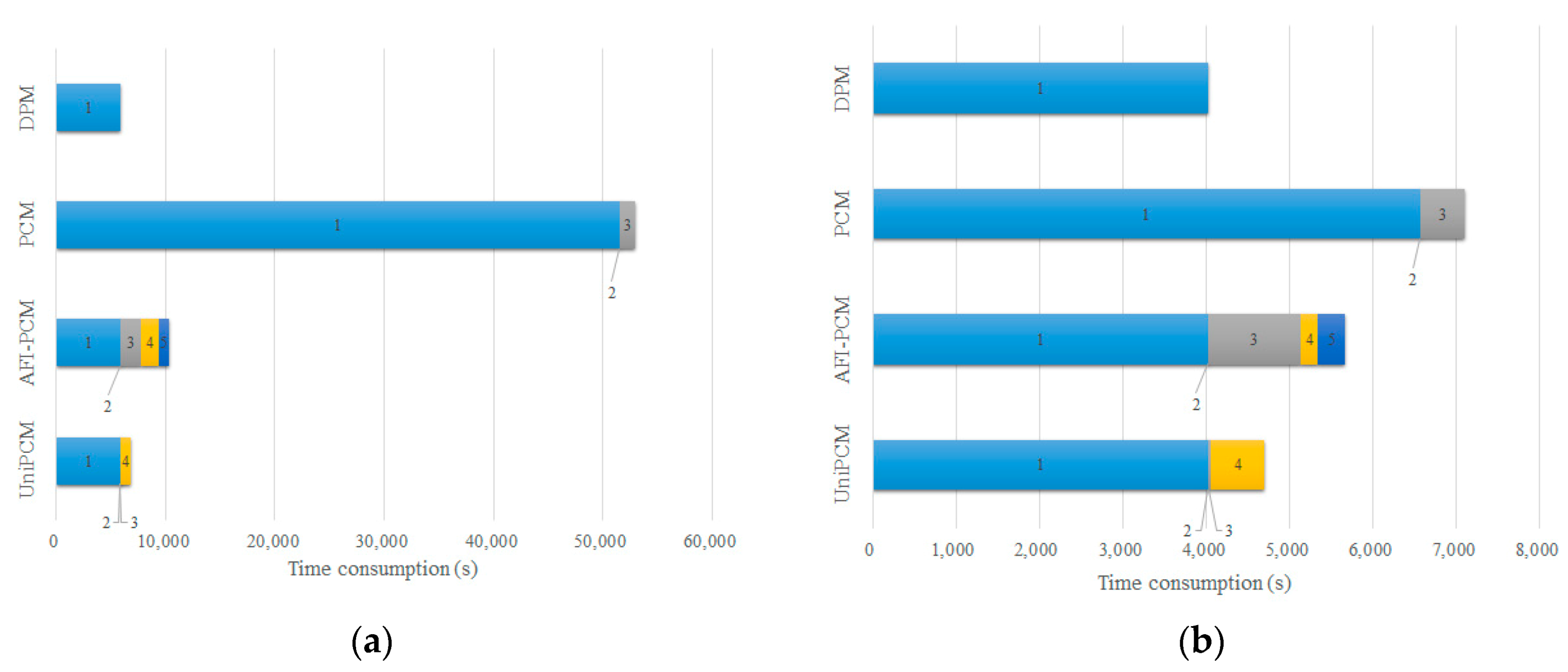
In this section, we only take the north direction of airplane and ship models as our experimental subjects. The statistical results of the model training stage of these methods are illustrated in the bar chart of
Figure 15. The overheads of training one DPM model for airplane and ship categories are 5844 s and 4022 s, respectively. Note that DPM has much lower detection accuracy compared with PCM based methods, although it achieves shorter time overheads since it is only the first training step of PCM based methods. Compared with PCM, AFI-PCM largely reduces the training volume to about 19% and 80% for the two categories, that is, a speedup up to 5.16× and 1.25×. The majority of saved time is the multi-DPM model training of PCM. Compared to AFI-PCM, UniPCM cuts down the training time by another 40% and 17%. Taking the airplane category as an example, step 3 of UniPCM is done within 15 s, while AFI-PCM takes about 1923 s. The step of weights learning, including scores preparation, is also decreased to about 983 s, while AFI-PCM takes about 2501 s. A similar performance acceleration can be also observed on the ship model training.
As the numbers of partial configurations in PCM and UniPCM are different, we take a second look at the speedup obtained by our UniPCM. To generate one partial configuration for airplanes and ships, AFI-PCM needs 15% and 48% of the time consumed by PCM, while UniPCM only uses nearly 10% and 40% of PCM, that is, a speedup of 10× and 2.5×, respectively. We will achieve greater speedup if more partial configurations are designed. This speedup for training is obvious, and it is convenient for the fast implementation to new categories of objects, let alone the time already saved for massive manual annotation work.
4.6. Detection Time Analysis
AFI-PCM and PCM simply detect
DPM models of partial configurations, that is, it is nearly
times of one single DPM detection. UniPCM only convolves through the image once and then directly obtains the responses of all partial configurations. To evaluate the more important detection speed, we obtain the statistical time consumption of PCM, AFI-PCM, and UniPCM for full-direction detection.
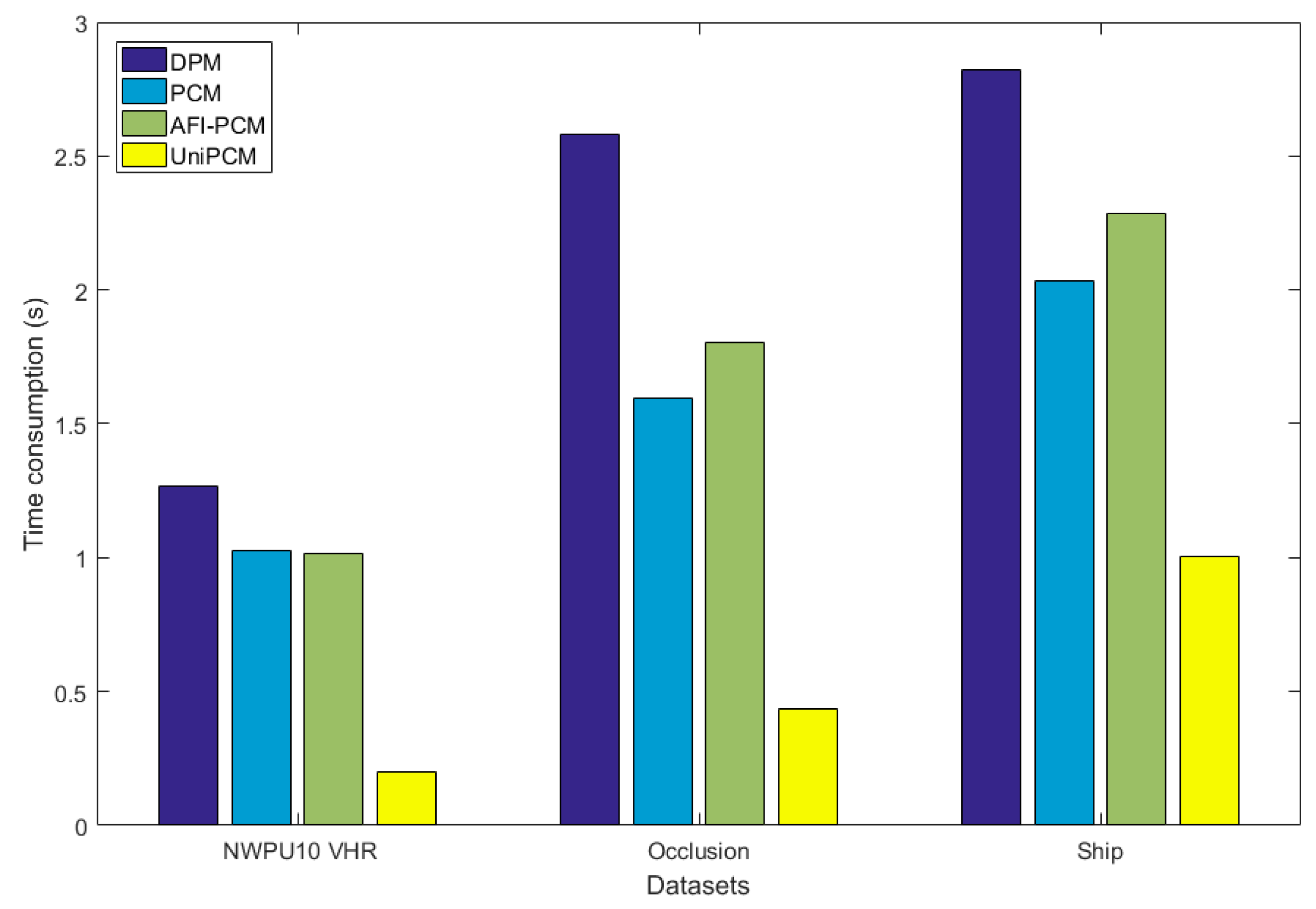
Figure 16 illustrates the time consumption per partial configuration per image of the three methods. The average image sizes of datasets are 683 × 970, 1125× 1457, and 987 × 1747. Similar to
Section 4.5, we give the detection time consumption of MSCNN of each image in the three datasets, which is about 0.15 s, 0.32 s, and 0.35 s, respectively.
Since a full-object DPM model generally has more filters than a single partial configuration, it takes the highest time consumption among all baselines as in
Figure 2, which partially supports that obtaining the filter responses takes great detection time. As indicated in
Figure 2, nearly three quarters of AFI-PCM and PCM detection computation involves calculating for the responses of filters. Although AFI-PCM shares the parts between partial configurations, their filter responses are actually wasted and unshared during detection. UniPCM makes full use of these responses and its total time consumption for one partial configuration is only 0.2 s for NWPU10 VHR, 0.4 s for Occlusion, and one second for Ship dataset; this is almost only 14%, 24%, and 40% of AFI-PCM, respectively, that is, a speedup up to 7.2×, 4.1× and 2.5× over AFI-PCM, and 5.1×, 3.7× and 2× over PCM. UniPCM makes fast POOD become possible. The detection speeds of AFI-PCM and PCM are roughly the same, with differences mainly coming from the extra weights multiplication in AFI-PCM.
To achieve full-direction detection of objects in the experiment, AFI-PCM and UniPCM maintain 208 and 188 partial configurations for the categories of airplane and ship, while PCM uses 160 and 48 partial configurations. It can also be inferred from
Figure 16 that when more partial configurations are designed, UniPCM will obtain a much higher detection speedup.


