Article

Evaluating the Applications of the Near-Infrared Region in Mapping Foliar N in the Miombo Woodlands

1
Discipline of Geography, School of Agricultural, Earth and Environmental Sciences, University of KwaZulu-Natal, P/Bag X01, Scottsville, Pietermaritzburg 3209, South Africa
2
Department of Physics, Geography and Environmental Science, Great Zimbabwe University, P.O. Box 1235, Masvingo 00263, Zimbabwe
3
Department of Geography & Environmental Science, University of Zimbabwe, P.O. Box MP 167, Mount Pleasant, Harare 00263, Zimbabwe
*
Author to whom correspondence should be addressed.
Remote Sens. 2018, 10(4), 505; https://doi.org/10.3390/rs10040505
Submission received: 23 November 2017 / Revised: 13 January 2018 / Accepted: 20 January 2018 / Published: 23 March 2018

Abstract

:
Remote sensing has been widely used to estimate the distribution of foliar nitrogen (N) in a cost-effective manner. Although hyperspectral remote sensing targeting the red edge and shortwave infrared regions has proved successful at estimating foliar N, research has recently shifted to include exploring the benefits of using the near-infrared (NIR) region, especially when using broadband sensing. Bootstrapped random forest regression analysis was applied on Sentinel 2 data to test the significance of using the NIR in foliar N estimation in miombo woodlands. The results revealed a low ranking for individual NIR bands, but the ranking improved when spectral indices were used. In addition, the results indicated a marginal increase in the normalised root mean square error of prediction (nRMSE) from 11.35% N when all bands were used to 11.69% N when the NIR bands were excluded from the model. Bootstrapping results show higher accuracy and better consistency in the prediction of foliar N using combined spectral indices and individual bands. This study therefore underscores the significance of spectral indices to increase the NIR region’s importance in estimating the distribution of foliar N as a key indicator of ecosystem health at the landscape scale in miombo systems.

Graphical Abstract

1. Introduction

In natural ecosystems, such as the miombo woodlands, nitrogen (N) regulates several key processes, such as plant productivity [1,2], rates of litter decomposition, and dynamics of the terrestrial carbon cycle [3]. The remote estimation of foliar N, a key component of plant biochemistry, is therefore invaluable in the mapping and monitoring of ecosystem health. The major advantage of using remote sensing technology in estimating foliar N is cost-effectiveness, owing to its capability to give synoptic, repetitive, and objective observations of the earth’s surface [4].
The remote estimation of foliar biochemicals is based on Beer’s Law [5], which predicts how the amount of absorbed or reflected electromagnetic radiation is directly related to foliar chemical concentrations. However, unlike chemical extracts used in laboratory setups, pigments from field samples are integrally bound with leaf structure; therefore, reflectance is not a function of the chemicals alone [6]. Despite this challenge, some regions of the electromagnetic spectrum have emerged as important in the remote estimation of foliar biochemical constituents. For example, the red edge region has been shown to be highly correlated to foliar N at the field level [7,8,9,10,11,12,13]. These studies succeeded in estimating foliar N by exploiting the strong relationship which exists between red edge reflectance and chlorophyll concentration, which holds a significant amount of leaf N. Despite the strong relationship between red edge reflectance and leaf N, the spatial extent of remote sensing methods of estimating N were limited by the low spatial coverage of the hyperspectral imagery [14]. Furthermore, the water absorption features in the shortwave infrared (SWIR) region were also found to mask the N absorption regions [15,16]. At the landscape scale, an increased absorption of radiation in the SWIR due to multi-layering of tree canopies further compounds the challenges of mapping foliar N. Thus, there is still a need to develop methods that can be used to estimate foliar N at the landscape level.
The application of broadband imagery has emerged as a promising method of estimating N at a landscape level [14,17]. Previous studies have successfully applied multispectral imagery in estimating foliar biochemicals using the near-infrared (NIR) region [18,19,20], including N [3,14,21]. These studies were mainly conducted in agro-ecosystems and temperate forests and had R2 values averaging around 0.80. The remote estimation of foliar N using the NIR region is based on the spectral properties of total lignin, cellulose, and N [22]. Reflectance in the NIR region is also a function of biomass, leaf area index, and leaf thickness; properties which are all affected by leaf N [14]. The establishment of a functional relationship between NIR and foliar N is considered the missing link to the generalised estimation of NIR using broadband satellites [17,23]. A recent study has hinted at the existence of a relationship between vegetation albedo and canopy N, which creates new opportunities for the remote estimation of N using broadband imagery [20]. The authors in [24] proposed a generalised partial least squares (PLS) model that relates NIR reflectance to foliar N across different ecosystems. This model rides on the observed consistent performance of the NIR region in estimating foliar N across temperate, humid tropical, and boreal forests. However, the low spatial coverage of imaging spectrometers has limited the subsequent development and testing of such universal models [14]. Despite the recorded progress, some scepticism, for example [25], still exists in using broadband imagery for N estimation. They argued that the relationship between foliar N and NIR is spurious, and is a function of canopy configuration rather than N concentration. However, when fully developed, NIR methods of estimating N using broadband satellites have the potential of landscape level estimation of leaf N.
The miombo woodlands cover an estimated 2.7 million km2 in central and southern Africa [26,27], and are one of the most extensive seasonally humid forest vegetation types in Africa. They are dominated by three genera of Julbernardia, Brachystegia, and Isoberlinia, which are seldom found outside the woodlands [26]. The miombo ecoregion, which is often confused with the woodlands, is made up of the miombo woodlands and other associated species, such as Vachellia spp., Colophospermum mopane, Baikiaea spp., and Burkea-Terminalia spp., which often form their own extensive stands [28]. The drier miombo woodlands (<1000 mm annual rainfall) cover most of Zimbabwe, Mozambique, and the southern parts of Malawi. The wetter miombo occurs in Angola, Tanzania, Zambia, and central Malawi, in areas receiving above 1000 mm of rainfall [26,28]. The miombo woodlands support a variety of large mammals in Africa, including 50% of the threatened species population of the African elephant (Loxodonta africana) and the rhinoceros (Rhinocerotidae spp.) in Africa [26]. The miombo woodlands have been receiving increasing biodiversity conservation attention [29] owing to their vastness, high endemicity levels, and unique habitat status [26,27,30]. To date, no study has tested the utility of the new generation multispectral sensors for estimating the distribution of foliar N at landscape scales in the miombo systems.
In this study, we test the utility of using the NIR region in mapping foliar N in the miombo woodlands of southern Africa. Using random forest regression, we used the recently launched Sentinel-2 satellite data to investigate the significance of the NIR region (a) as individual bands and (b) contained within spectral indices in the estimation of foliar N.

2. Materials and Methods
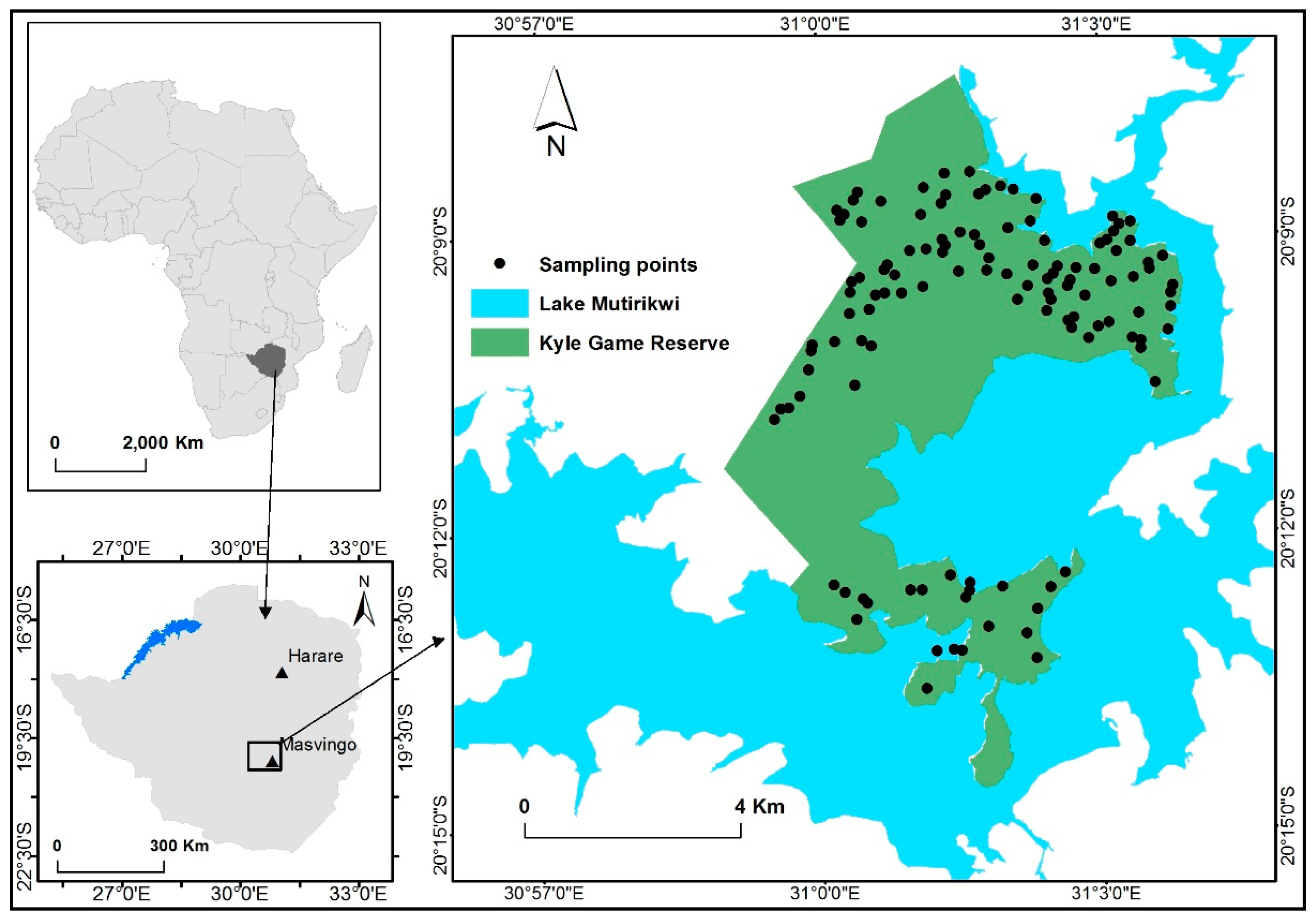
2.1. Study Area

The Kyle Game Reserve covers an area of approximately 44 km2. It was established as a recreational park in 1960 to conserve biological diversity. The game reserve is located between latitudes 20°04′ and 20°14′ South, and longitudes 31°07′ and 30°50′ East in southern Zimbabwe (Figure 1). It is situated about 56 km southeast of Masvingo city. The relief is dominated by the Beza mountain range and a plain that is dotted by a number of isolated hills, and stretches from the foot of the mountain range to the lake shore [31]. The altitude varies between 700 and 1485 m above sea level.
The climate is subtropical savanna, with an annual average rainfall of 622 mm (Masvingo airport rainfall data: 1906–2015). Most of the rain falls during a single wet (growing) season that stretches from mid-November to end of March. The mean daily maximum temperature ranges from 21 °C in June to 29 °C in October. The mean daily minimum temperatures range from 5 °C in July to 17 °C in January [32]. The soils comprise a mixture of chromic–leptic lixisols and chromic luvisols that are mainly derived from granitic and gneiss parent materials [33]. The vegetation on the plain ranges from miombo woodlands, dominated by msasa (Brachystegia spiciformis) and mnondo (Julbernardia globiflora), to bushland thickets dominated by African weeping wattle (Peltophorum africanum), Silver terminalia (Terminalia sericea), Combretum spp., and sweet thorn (Vachellia karoo), and to extensive grasslands dominated by thatch grass (Hyparrhenia filipendula), red grass (Themeda triandra), and yellow thatching grass (Hyperthelia dissoluta) [32,34].

2.2. Field Nitrogen Data

A field campaign was conducted from 4 April 2017 to 16 April 2017. This time coincided with the end of the growing season in the miombo woodlands. A landcover map of the game reserve, generated from a Sentinel-2 image of May 2016 with a kappa statistic of 0.83, was used to locate relatively homogenous miombo woodland stands that were targeted for sampling. Using the Hawths tools in ARCGIS 10.1 [35], a total of 103 sampling points distributed only in the miombo woodlands were generated (see Figure 1). A minimum distance of at least 150 m was set between sampling plots to eliminate the possibilities of overlapping pixels in the satellite image data. The coordinates (xy) of the sampling points were uploaded into a hand-held global positioning system (GPS) receiver.
In the field, a Garmin Etrex GPS receiver with a positional accuracy of ≤3 m was used to locate the random sampling points. Each sampling point was taken as the centre of a quadrat plot measuring 20 m by 20 m, which was north-oriented using a compass. A plot size of 400 m2 was chosen to coincide with the coarser spatial resolution of the Sentinel-2 data. The centroid of each sampling plot was located such that for a minimum distance of 40 m around the plot, the entire plot fell within a miombo woodland cover. This measure was taken to minimise the potential contaminating effect of other landcover types on the spectral value of the sampling plot.
In each sampling plot, all miombo trees whose canopies contributed most to the percentage canopy cover were identified and assigned a unique number. Those individual trees with the largest crowns (diameter >5 m) were targeted for sampling in each plot. The bigger and more widespread the crown of an individual tree, the greater its influence on the canopy cover of the sampling plot, and consequently the more influential it is on the reflectance value. Then, about 2–4 individual trees were randomly chosen. From each selected tree, 6 to 10 fresh, fully expanded green leaves [36] were clipped from two layers within the canopy; namely, the sunlit leaves from the top of the canopy and the partially shaded leaves from within the canopy. Our sampling plots were largely homogeneous, being dominated (>80%) by a single species of either Julbernardia globiflora or Brachystegia spiciformis. Consequently, the foliar samples were from the dominant tree species. At each sampling plot, leaves from the same canopy level but different trees were mixed to make one composite sample and placed in an airtight container, which was stored in a cooler box full of ice. At the end of each day, the collected samples were oven dried at 80 °C for 48 h. All leaf samples were later sent to the Department of Biological Sciences at the University of Zimbabwe in Harare for foliar N determination.
In the laboratory, the standard colorimetric method was used to determine foliar N concentration [37,38]. In brief, the plant material was first digested using selenium powder, lithium sulphate, hydrogen peroxide, and sulphuric acid [39,40]. Then, the absorbance of each sample was read using a Cole and Parmer 1100 spectrophotometer set at 655 nm. N concentration was expressed as a percentage of the dry matter. The colorimetric method has produced reliable results elsewhere hence its use [4,38,41]. The results for the top and middle canopy were analysed and presented separately. In this study, however, an average of the two values was related to remotely sensed data.

2.3. Remote Sensing Data

A Sentinel-2 level 1C image was downloaded from the European Space Agency (ESA) website [42]. The image was acquired on 12 April 2017, which coincided with the period of the field campaign. Sentinel-2 data consists of 13 bands, from the visible to the shortwave infrared band. Two of the bands contain information on cirrus clouds (band 10) and aerosols (band 1); therefore, they were not used in this study. An atmospheric correction procedure was performed on the Sentinel-2 data using the SACP plugin [43] in QGIS software, version 2.18. All of the bands were later re-sampled using the nearest neighbour analysis to the same 10 m spatial resolution in the SNAP software [44] to facilitate layer stacking during analysis. Table 1 presents the wavelength as well as spatial resolution of the Sentinel-2 bands used in this study.

2.4. Spectral Indices

In this study, eight spectral indices that were previously related to field N were calculated from Sentinel-2 data and used to estimate foliar N. The indices used, and the mathematical expressions applied to derive them, are given in Table 2. Five of the indices included the NIR band, while only three indices did not include the NIR band.

2.5. Random Forest Regression

We used the Random Forest (RF) regression model in relating (a) individual Sentinel-2 bands, (b) spectral indices, and (c) combined spectral indices and individual bands to field-measured foliar N. The RF regression model was used because of its ability to handle several input variables, such as remote sensing bands, while circumventing overfitting and multi-collinearity problems [4,51]. The RF regression analysis was performed in the R environment software developed by [52]. Specifically, the “randomForest” package developed by [53] was used to execute random forest regression. The RF regression algorithm is a bagging method that is based on the classification and regression trees (CART) method [4,51]. Three parameters were optimized: node size, mtry, and ntree, where the node size is the minimal size of the terminal nodes of the trees, mtry is the number of predictor variables performing the data partitioning at each node, and ntree is the total number of trees to be grown in the model [51]. The best ntree values for predicting foliar N in the miombo woodlands were determined by optimising ntree based on the root mean square error of calibration (RMSEC). The number of trees was tested from 100 to 1000 at intervals of 100 [54]. The default node size and mtry were accepted throughout the analysis. A more detailed explanation of random forest is outlined elsewhere [4,55,56].
The RF regression model was also applied to assess the importance of the NIR in the prediction of foliar N. Prior to running the model, the data set was randomly partitioned into modelling and validation data based on a 70:30 ratio (72 and 31 sampling points, respectively). The importance of each predictor variable was measured by calculating the percent increase in mean squared error (%IncMSE) when data not used in the prediction (out of the bag (OOB) data) for each variable are permuted, while all others are unchanged [54]. The mean variable importance was calculated from 500 bootstraps, and the results were shown. Bootstrapping is a resampling procedure that randomly selects samples with replacement, allowing researchers to draw conclusions from the existing sample rather than by making assumptions about the estimator [57]. In this study, each bootstrap iteration drew 72 plots with replacement from the 72 available samples. The remainder of the samples that were not drawn for modelling were used as holdout samples for an independent validation [58]. The mean percent increase in mean square error was used to rank the importance of (a) individual sentinel-2 bands and (b) each spectral index in predicting foliar N in the miombo woodlands. The variable with the highest ranking was the most important variable for predicting foliar N. After ranking the individual bands and spectral indices, we generated two more random forest models, which excluded (a) the NIR band (from the individual band list) and (b) those spectral indices which have information from the NIR band.

2.6. Model Evaluation

In order to evaluate the performance of the five random forest models, we made use of three statistical parameters. These are the normalised root mean square error (nRMSE), a square of the strength of the correlation (r2) between the observed and predicted values, and the bias. Firstly, the RF models were calibrated using the individual bands and spectral indices. A bootstrapping procedure with 500 iterations was then applied on the random forest regression models to predict the value of N from an independent test dataset of 31 observations. The mean nRMSE, mean r2, and mean bias from the 500 bootstraps were calculated for each of the five RF models and were used as measures of accuracy of the RF models. Based on the nRMSE, the best RF model was used to produce a map of the mean N and standard deviation of N based on the 500 bootstraps.

3. Results

The field-measured foliar N was variable. It ranged from a minimum of 0.33% to a maximum of 5.33%. The mean N concentration in the study area was 2.43%, with a standard deviation of 1.07%.

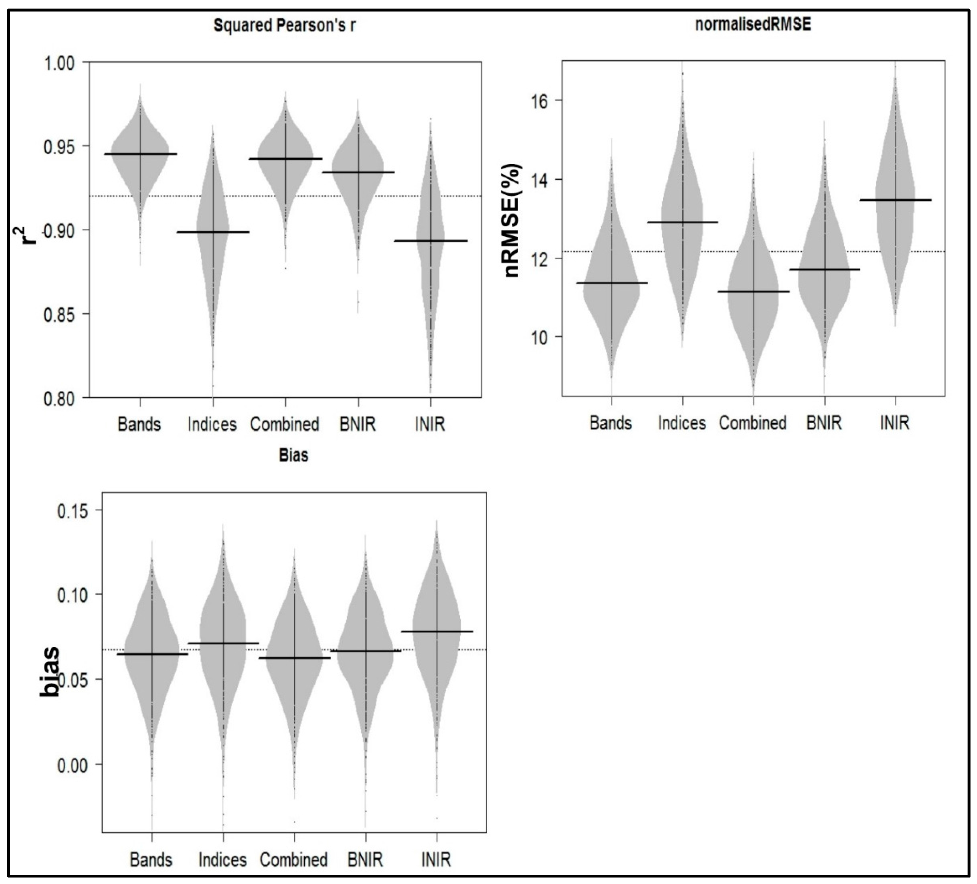
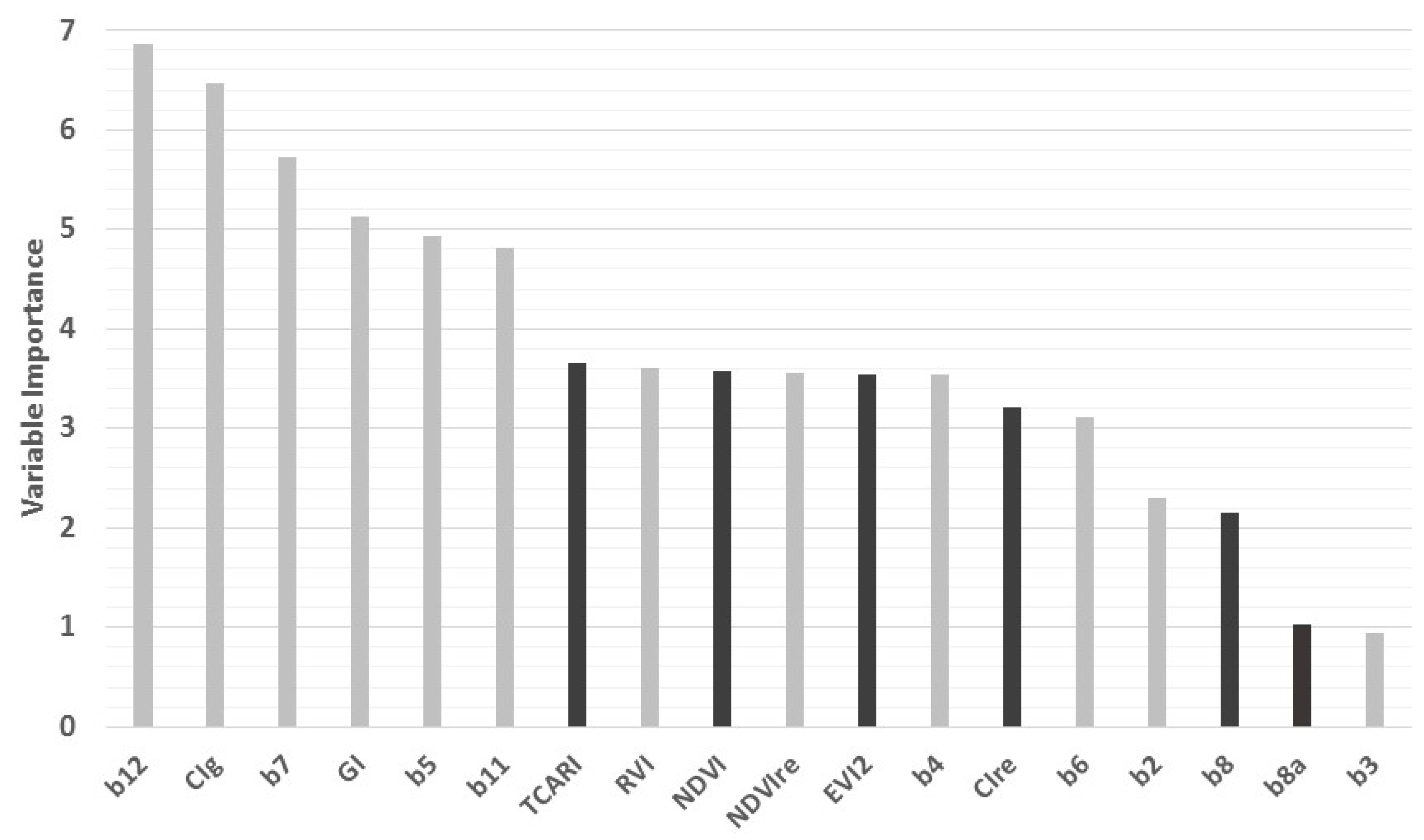
3.1. Individual Bands

Results of this study show that the NIR region of the electromagnetic spectrum is ranked lowly in the prediction of foliar N in the miombo woodlands. Figure 2 shows that the NIR band (band 8), the best-ranked NIR band in predicting foliar N, is ranked eighth out of the ten bands that were considered. The other NIR band (band 8a) is ranked ninth, which is second from last. The results in Figure 2 indicate that the four most important bands are found within the red edge section of the electromagnetic spectrum (band 5 and band 7) as well as the shortwave infrared (SWIR) portions of the electromagnetic spectrum (band 11 and band 12). The fifth-most important band is the blue band (band 2). The other red edge band (band 6) is ranked lowly in the prediction of foliar N in the miombo woodlands.

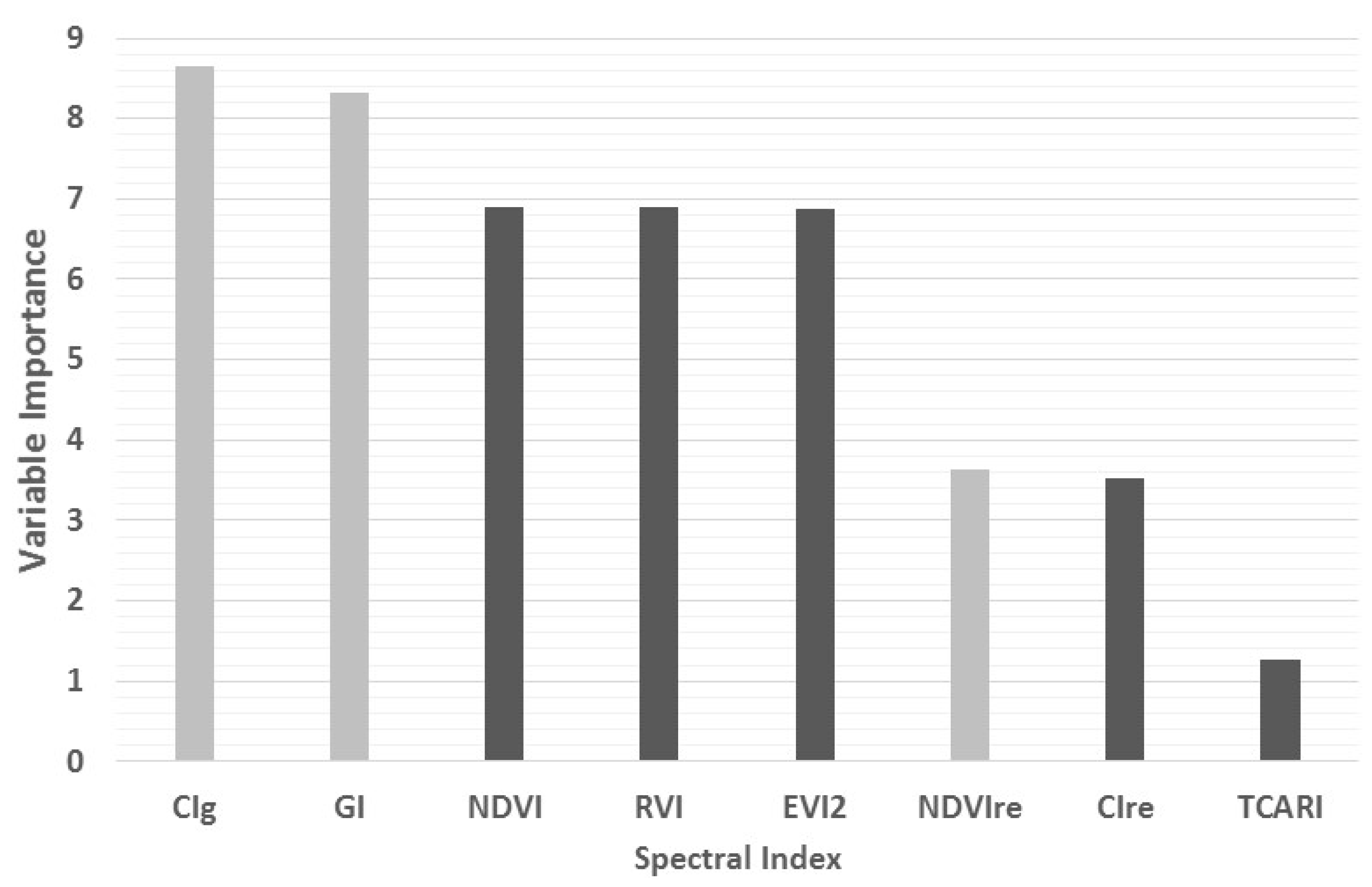
3.2. Spectral Indices

Figure 3 illustrates that three of the five most important spectral indices for estimating foliar N (that is, simple ratio index (RVI), enhanced vegetation index (EVI), and normalised difference vegetation index (NDVI)) contain the NIR band. Specifically, NDVI, which is derived from the NIR and red bands, is the most important NIR-based spectral index for predicting variations in foliar N concentration in the miombo woodlands. The two spectral indices ranked higher than NDVI are the green chlorophyll index (CIG) and the green index (GI), both of which contain the green band. Only the CIG contains information from the red edge band. The spectral index containing only the red edge (NDVIre) was ranked lower than several spectral indices which contained the NIR and visible region bands. When combined in a spectral index, the NIR band improved in their ranking in foliar N prediction. However, combining the individual bands and spectral indices in the same model results in a low ranking of the NIR-based indices (Figure 4). This shows the low ranking of information from the NIR region in predicting N in the miombo woodlands.

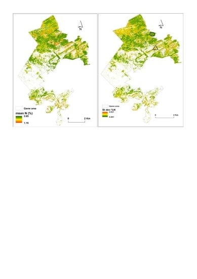
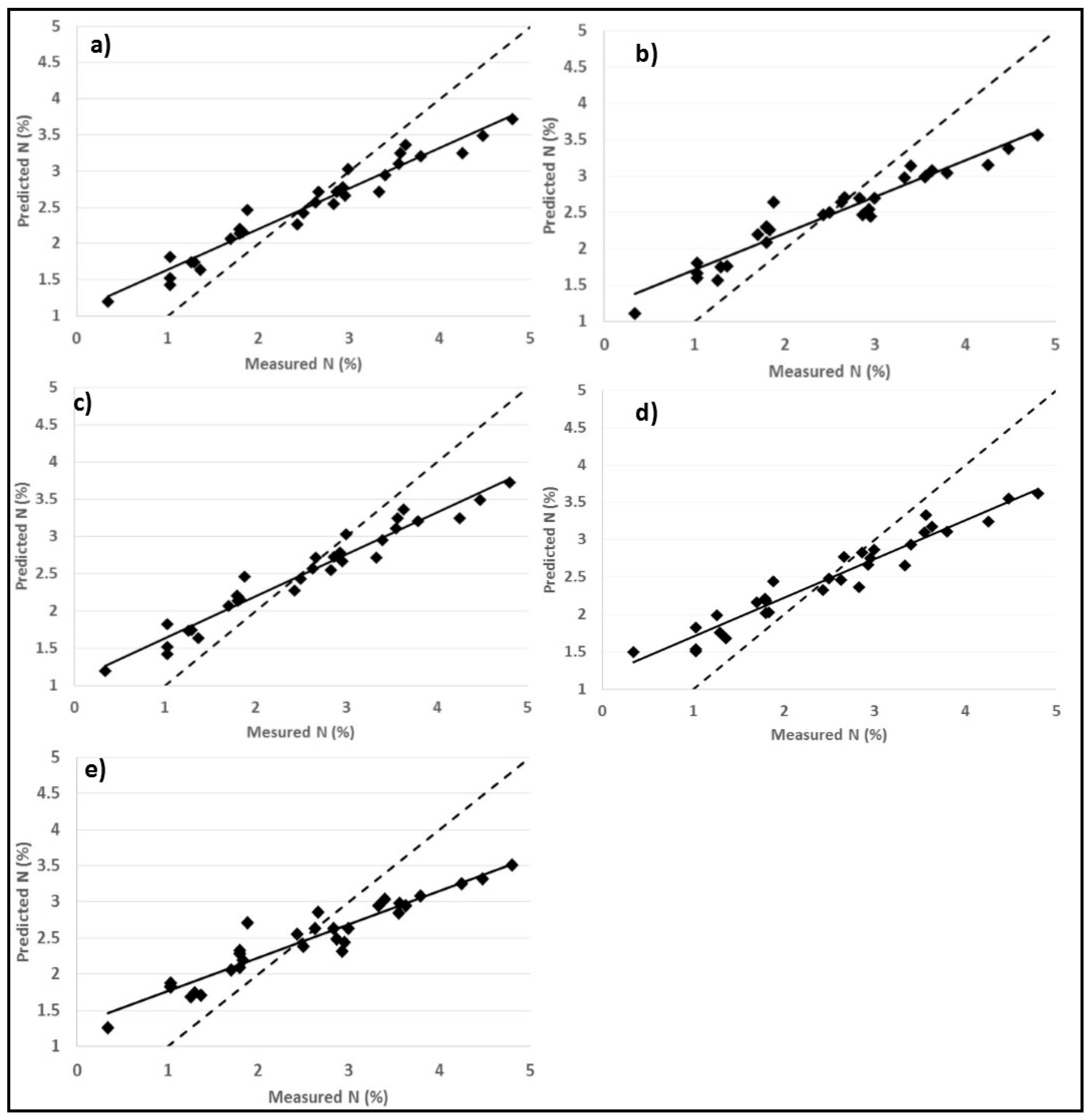
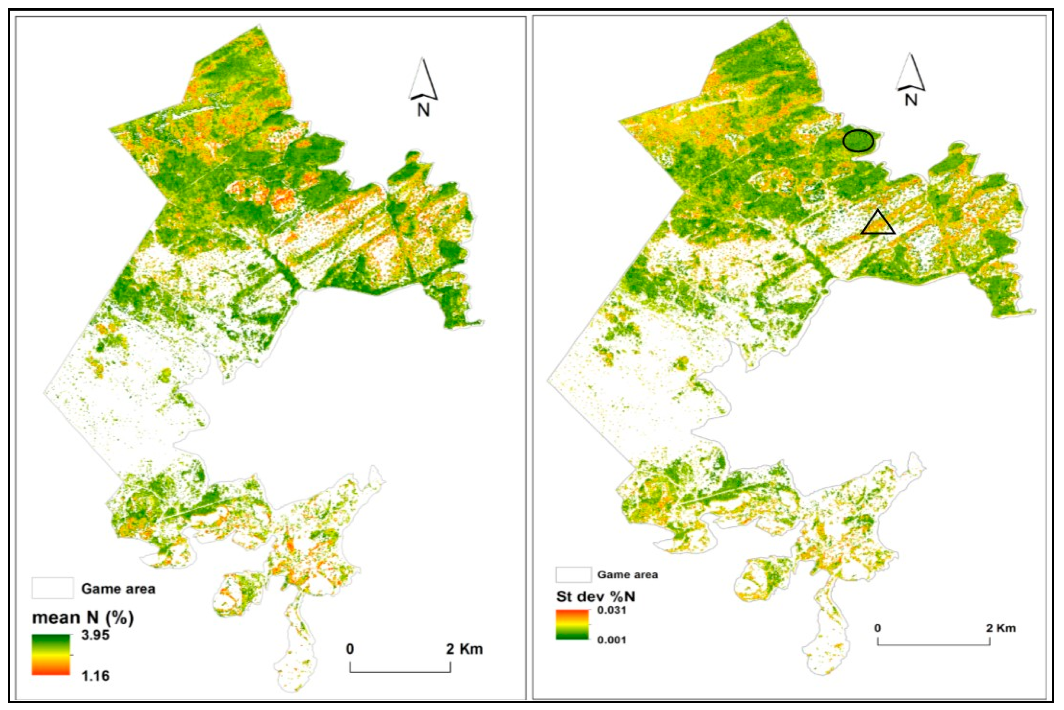
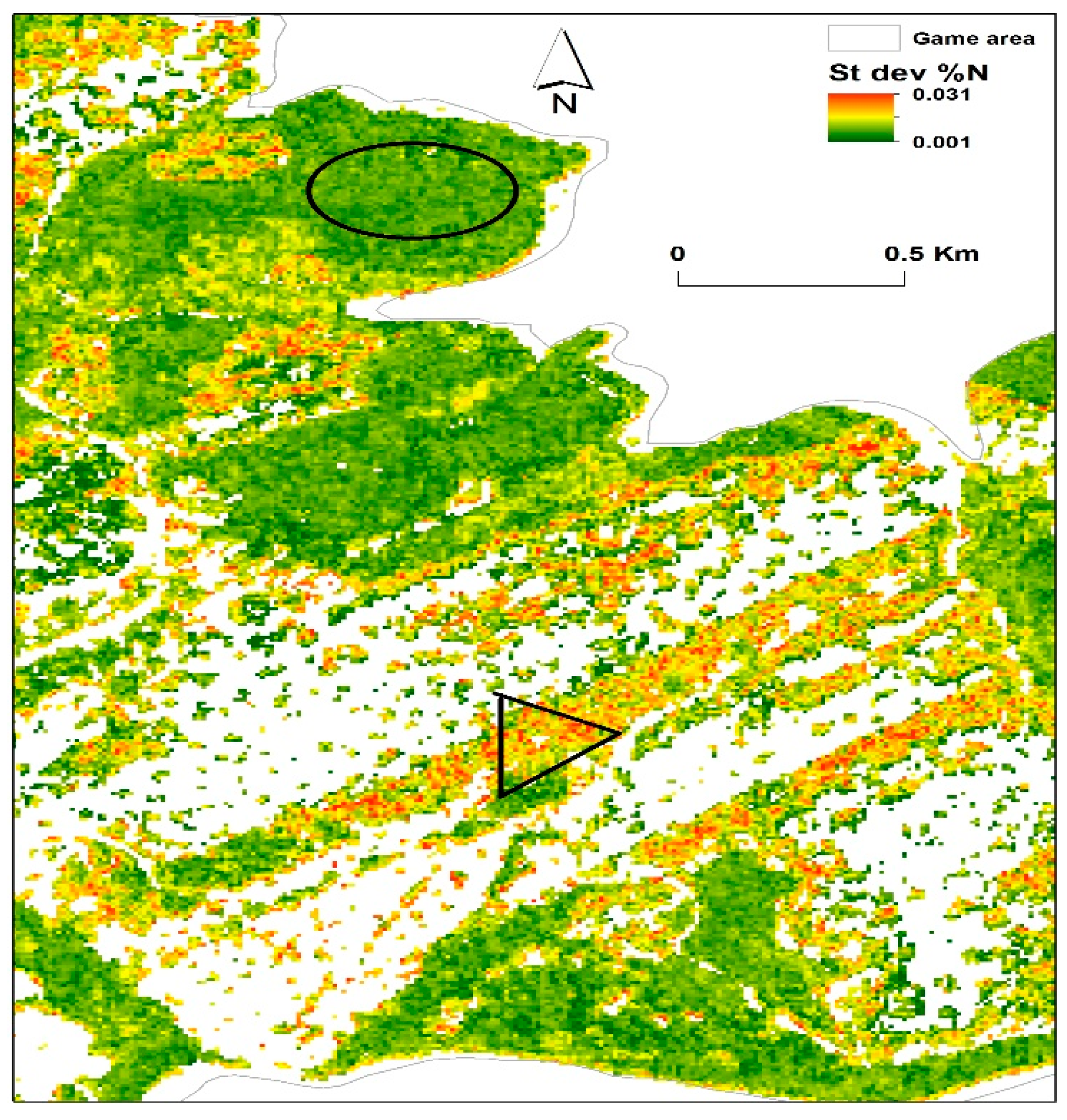
3.3. Predictions of Foliar N

Table 3 shows that individually, the NIR band makes a small contribution in the prediction of foliar N in the miombo woodlands.
A comparison of the two models utilising individual Sentinel-2 bands revealed that an exclusion of the NIR bands in the random forest regression model increased the normalised root mean square error (nRMSE) from 11.35% to 11.69%. The coefficient of determination of the model marginally dropped from 0.94 to 0.93. On the other hand, it can be noted that excluding NIR-based spectral indices resulted in a marginal decline in the value of r2, while the normalised root mean square error increases from 12.90% to 13.45%. The marginal decrease in the r2 when NIR-based indices were excluded from the model points towards the significance of using spectral indices in the prediction of foliar N in the miombo woodlands. Combining both individual bands and spectral indices in the regression model resulted in the lowest nRMSE recorded.
Scatterplots of the relationship between predicted N and field-measured N are shown in Figure 5. The scatterplots show a generally consistent deviation from the 1:1 line by all the models. Figure 5 shows that there is an overestimation of foliar N at lower concentrations. At higher concentrations of N, there is an underestimation of foliar N. The goodness of fit statistics for the relationship between predicted N and field-measured N are given in Table 3.
Figure 6 shows the distribution of the accuracy statistics of the five models after running a bootstrap with 500 iterations. Figure 6 shows that for the three accuracy statistics, the bias was the least varied, while the r2 and the nRMSE were highly variable (more widely spread). While the nRMSE for the two models based on spectral indices was consistently high, the r2 for the same models was low. The higher nRMSE indicates a lower prediction accuracy, while the wider range of values indicate increased variation in the performance of the models in predicting foliar N. Models utilising individual bands on the other hand have a narrower range of values, indicating a more consistent prediction of foliar N in the miombo woodlands.
Figure 7 shows the spatial variation of mean %N in the miombo woodlands estimated using the RF model developed from all the individual bands and spectral indices. This model was chosen because it had the lowest nRMSE (Table 3).
The map of the standard deviation in Figure 6 shows very low variation (0.001 to 0.031) in the prediction of foliar N. The low values of standard deviation are consistent with the results from Figure 6, where the combined model shows a narrower range of values of nRMSE. Figure 8 shows areas of high and low standard deviation of foliar N prediction using the RF model with all the spectral indices and all individual bands.
The areas that have a lower standard deviation (black oval in Figure 8) have more mature trees and a higher percentage cover, while those areas that have a higher standard deviation (black triangle in Figure 8) have lower percent canopy cover. The higher variations in predicted figures might be explained by the inclusion and exclusion of such sample plots in the calibration of the model, thereby altering the accuracy of the model. The soil background could also have affected the prediction accuracy, causing higher uncertainty in sample plots of medium canopy cover. The absence of the soil background in sample plots of high canopy cover could have led to small variations in the prediction of foliar N.

4. Discussion

The results demonstrate that, when single bands are used, information from the NIR region ranked very lowly in the prediction of foliar N within the miombo woodlands. Our results contradict several studies that have ranked the NIR region highly in predicting variations in foliar N [14,22,59,60]. For example, [61] concluded that the NIR band significantly (r2 = 0.73) predicted variation in foliar N in the Bavarian Forest National Park, a mixed temperate forest ecosystem. In addition, Lepine et al. [14] also reported an r2 of 0.86 when relating foliar N to the NIR bands. However, in this study, the red edge and the SWIR regions are important in the prediction of N when we consider individual bands. However, the spectral indices containing the NIR and red regions were found to be important in the prediction of foliar N in the miombo woodlands.
Another important feature of the findings is that, when spectral indices are used, the indices which contained the NIR band, such as RVI and EVI2, ranked highly in the prediction of N in the miombo woodlands. This result provides additional empirical support to the hypothesis that spectral indices increase the content of the information in remotely sensed data and the NIR gains in importance when combined with other bands. The three best predicting spectral indices that contain the NIR are made up of the NIR and the red band, showing the prominence of the visible region in the estimation of N. The superior performance of the spectral indices derived from the NIR can be attributed to the fact that spectral indices generate new information by aggregating the relationships between foliar N and different portions of the electromagnetic spectrum [62]. The NIR region contains information on several leaf characteristics, including biomass, leaf area, and thickness [14], while the red edge is related to chlorophyll concentration; leaf properties which have both been related to foliar N concentration [11,17]. Spectral indices have evolved over time with the aim of enhancing the vegetation signal while decreasing the “noise effect” from several sources, including solar irradiance and soil background [63]. However, other critical factors, such as the leaf area index [64] and saturation problems, have to be accounted for if the spectral indices are to be used for mapping foliar biochemicals such as N.
Results of this miombo study share similarities with some studies that were carried out in grassland ecosystems of southern Africa at the landscape scale. For example, [65] used simulated Sentinel-2 data and came to the conclusion that the red edge and SWIR bands were significant in remotely estimating foliar N in a savanna grassland. In addition, the visible SWIR bands (583 nm, 679 nm, 710 nm, 2091 nm, 2128 nm, and 2146 nm) and red edge position were also important in predicting foliar N in Colophospermum mopane woodlands [66,67]. Our study is different in that the previous studies used hyperspectral remote sensing as well as simulated Sentinel-2 bands to relate to foliar N, where here broadband Sentinel-2 images were used in estimating foliar N. The high ranking of the red edge in this study is not surprising. This is because the red edge has been widely used in mapping leaf biochemical composition across different ecosystems [8,11,68,69]. However, the consistency in the importance of the SWIR region underlines its significance for foliar N estimation in seasonally humid landscapes. The SWIR region contains N absorption features that have been used in the remote estimation of N [15,16,21,70]. The development of SWIR-based methods, however, has been overshadowed by those from the red edge region mainly because the N absorption features in the SWIR are masked by water absorption.
The application of spectral indices containing NIR as well as the SWIR in foliar N mapping is a promising method of using broadband remote sensing in estimating N at the landscape level. On one hand, Ref. [14] noted that the %N–NIR relationship is driven by several canopy structural properties that influence reflectance. On the other hand, Pellissier et al. [71] concluded that the NIR and SWIR peaks that explained %N variations were also significant in explaining variations in canopy height, biomass, and water content. Taking these two conclusions together, other factors, such as water availability in an ecosystem, can potentially influence the relationship between foliar N and NIR. This is important given that the SWIR region contains both water and N absorption features [72,73]. However, information from the NIR region has ordinarily been used to explain leaf characteristics such as leaf area index, density, and canopy cover [14]. While our study was conducted within the miombo woodlands, within a single season, the results provide an insight into the remote estimation of foliar N in other resource-constrained environments where hyperspectral remote sensing is considered too expensive and broadband remote sensing is an alternative.

5. Conclusions

This study assessed the utility of the NIR region in estimating foliar N in the miombo woodlands. This study concluded that when used as single bands, the NIR region is ranked low when related to foliar N in the miombo woodlands. However, when combined with other bands in spectral indices, the importance of the NIR region improved markedly. This means that spectral indices which contain the NIR band are important in the estimation of foliar N in the miombo woodlands. This finding suggests that combining bands generates new information which is important in the prediction of foliar N in the miombo woodlands. Spectral indices improve the relationship between foliar N and remotely sensed imagery by minimising the “noise” in spectral values while amplifying the relationship with factors affecting leaf morphology, such as biochemicals. Information from a single broadband channel is often too “contaminated” to be meaningfully related to variations in foliar biochemical concentrations, including N.
Sentinel-2 broadband data has been proved to be very useful in foliar N mapping. The spatial resolution of 20 m potentially offers no challenges in less-frequently disturbed ecosystems. This is largely because few individual trees dominate the reflectance, making field sampling cheaper and correlation with field data easier. However, in frequently disturbed ecosystems made up of several smaller individual trees, relating reflectance to foliar N may be costly and compounded by the presence of several species. This method is significant in the mapping and monitoring of foliar N as a measure of ecosystem health in the miombo woodlands.

Acknowledgments

The authors are grateful to the anonymous reviewers whose comments improved this manuscript.

Author Contributions

Godfrey Mutowo conceived the research, collected data, analysed the data, and wrote the paper under the supervision of Onisimo Mutanga and Mhosisi Masocha. Onisimo Mutanga and Mhosisi Masocha also edited the manuscript. Furthermore, Onisimo Mutanga provided the funds for open access publication.

Conflicts of Interest

The authors declare no conflict of interest.

References

  1. Asner, G.P.; Martin, R.E. Spectral and chemical analysis of tropical forests: Scaling from leaf to canopy levels. Remote Sens. Environ. 2008, 112, 3958–3970. [Google Scholar] [CrossRef]
  2. Cho, M.A.; Ramoelo, A.; Debba, P.; Mutanga, O.; Mathieu, R.; Van Deventer, H.; Ndlovu, N. Assessing the effects of subtropical forest fragmentation on leaf nitrogen distribution using remote sensing data. Landsc. Ecol. 2013, 28, 1479–1491. [Google Scholar] [CrossRef]
  3. Clevers, J.G.P.W.; Gitelson, A.A. Remote estimation of crop and grass chlorophyll and nitrogen content using red-edge bands on Sentinel-2 and -3. Int. J. Appl. Earth Obs. Geoinf. 2013, 23, 344–351. [Google Scholar] [CrossRef]
  4. Ramoelo, A.; Cho, M.A.; Mathieu, R.; Madonsela, S.; Kerchove, R.V.D.; Kaszta, Z.; Wolff, E. Monitoring grass nutrients and biomass as indicators of rangelandquality and quantity using random forest modelling and WorldView-2data. Int. J. Appl. Earth Obs. Geoinf. 2015, 43, 43–54. [Google Scholar] [CrossRef]
  5. Bortolot, Z.; Wynne, R. A method for predicting fresh green leaf nitrogen concentrations from shortwave infrared reflectance spectra acquired at the canopy level that requires no in situ nitrogen data. Int. J. Remote Sens. 2003, 24, 619–624. [Google Scholar] [CrossRef]
  6. Gamon, J.A.; Surfus, J.S. Assessing leaf pigment content and activity with a reflectometer. New Phytol. 1999, 143, 105–117. [Google Scholar] [CrossRef]
  7. Curran, P.J.; Dungan, J.L.; Gholz, H.L. Exploring the relationship between reflectance red edge and chlorophyll content in slash pine. Tree Physiol. 1990, 7, 33–48. [Google Scholar] [CrossRef] [PubMed]
  8. Filella, I.; Peruelas, J. The red edge position and shape as indicators of plant chlorophyll content, biomass and hydric status. Int. J. Remote Sens. 1994, 15, 1459–1470. [Google Scholar] [CrossRef]
  9. Barnes, E.M.; Clarke, T.R.; Richards, S.E.; Colaizzi, P.D.; Haberland, J.; Kostrzewski, M.; Waller, P.; Choi, C.; Riley, E.; Thompson, T.; et al. Coincident detection of crop water stress, nitrogen status and canopy density using ground-based multispectral data. In Proceedings of the 5th International Conference on Precision Agriculture, Bloomington, MN, USA, 16–19 July 2000. [Google Scholar]
  10. Baranoski, G.V.G.; Rokne, J.G. A practical approach for estimating the red edge position of plant leaf reflectance. Int. J. Remote Sens. 2005, 26, 503–521. [Google Scholar] [CrossRef]
  11. Mutanga, O.; Skidmore, A.K. Red edge shift and biochemical content in grass canopies. ISPRS J. Photogramm. Remote Sens. 2007, 62, 34–42. [Google Scholar] [CrossRef]
  12. Kanke, Y.; Raun, W.; Solie, J.; Stone, M.; Taylor, R. Red edge as a potential index for detecting differences in plant nitrogen status in whinter wheat. J. Plant Nutr. 2012, 35, 1526–1541. [Google Scholar] [CrossRef]
  13. Ramoelo, A.; Skidmore, A.K.; Cho, M.A.; Schlerf, M.; Mathieu, R.; Heitkönig, I.M.A. Regional estimation of savanna grass nitrogen using the red-edge band of the spaceborne Rapid Eye sensor. Int. J. Appl. Earth Obs. Geoinf. 2012, 19, 151–162. [Google Scholar] [CrossRef]
  14. Lepine, L.C.; Ollinger, S.V.; Ouimette, A.P.; Martin, M.E. Examining spectral reflectance features related to foliar nitrogen in forests: Implications for broad-scale nitrogen mapping. Remote Sens. Environ. 2016, 173, 174–186. [Google Scholar] [CrossRef]
  15. Curran, P.J. Remote Sensing of Foliar Chemistry. Remote Sens. Environ. 1989, 30, 271–278. [Google Scholar] [CrossRef]
  16. Herrmann, I.; Karnieli, A.; Bonfil, D.; Cohen, Y.; Alchanatis, V. SWIR-based spectral indices for assessing nitrogen content in potato fields. Int. J. Remote Sens. 2010, 31, 5127–5143. [Google Scholar] [CrossRef]
  17. Ollinger, S.V.; Reich, P.B.; Frolking, S.; Lepine, L.C.; Hollinger, D.Y.; Richardson, A.D. Nitrogen cycling, forest canopy reflectance, and emergent properties of ecosystems. Proc. Natl. Acad. Sci. USA 2013, 110, E2437. [Google Scholar] [CrossRef] [PubMed]
  18. Gamon, J.A.; Field, C.B.; Goulden, M.L.; Griffin, K.L.; Hartley, A.E.; Joel, G.; Penuelas, J.; Valentini, R. Relationships between NDVI, canopy structure, and photosynthesis in three Californian vegetation types. Ecol. Appl. 1995, 5, 28–41. [Google Scholar] [CrossRef]
  19. Zhao, C.; Liu, L.; Wang, J.; Huang, W.; Song, X.; Li, C. Predicting grain protein content of winter wheat using remote sensing data based on nitrogen status and water stress. Int. J. Appl. Earth Obs. Geoinf. 2005, 7, 1–9. [Google Scholar] [CrossRef]
  20. Hollinger, D.Y.; Ollinger, S.V.; Richardson, A.D.; Meyers, T.P.; Dail, D.B.; Martin, M.E.; Scott, N.A.; Arkebauer, T.J.; Baldocchi, D.D.; Clark, K.L.; et al. Albedo estimates for land surface models and support for a new paradigm based on foliage nitrogen concentration. Glob. Chang. Biol. 2010, 16, 696–710. [Google Scholar] [CrossRef]
  21. Wang, L.; Wei, Y. Revised normalized difference nitrogen index (NDNI) for estimating canopy nitrogen concentration in wetlands. Int. J. Light Electron Opt. 2016, 127, 7676–7688. [Google Scholar] [CrossRef]
  22. Aitkenhead-Peterson, J.A.; Alexander, J.E.; Albrechtova, J.; Kram, P.; Rock, B.; Cudlín, P.; Hruška, J.; Lhotakova, Z.; Huntley, R.; Oulehle, F.; et al. Linking foliar chemistry to forest floor solid and solution phase organic C and N in Picea abies [L.] Karst stands in northern Bohemia. Plant Soil 2006, 283, 187–201. [Google Scholar] [CrossRef]
  23. Ollinger, S.V.; Richardson, A.D.; Martin, M.E.; Hollinger, D.Y.; Frolking, S.; Reich, P.B.; Plourde, L.C.; Katul, G.G.; Munger, J.W.; Oren, R.; et al. Canopy nitrogen, carbon assimilation and albedo in temperate and boreal forests: Functional relations and potential climate feedbacks. PNAS 2008, 105, 19335–19340. [Google Scholar] [CrossRef] [PubMed]
  24. Martin, M.E.; Plourde, L.C.; Ollinger, S.V.; Smith, M.; McNeil, B.E. A generalizable method for remote sensing of canopy nitrogen across a wide range of forest ecosystems. Remote Sens. Environ. 2008, 112, 3511–3519. [Google Scholar] [CrossRef]
  25. Knyazikhin, Y.; Schull, M.A.; Stenberg, P.; Mõttus, M.; Rautiainen, M.; Yang, Y.; Marshak, A.; Carmona, P.L.; Kaufmann, R.K.; Lewis, P.; et al. Hyperspectral remote sensing of foliar nitrogen content. PNAS 2013, 110, 811–812. [Google Scholar] [CrossRef] [PubMed]
  26. Byers, A. Conserving the miombo ecoregion. In Reconnaissance Summary; WWF, Southern Africa Regional Program Office: Harare, Zimbabwe, 2001; p. 24. [Google Scholar]
  27. Jew, E.K.; Dougill, A.J.; Sallu, S.M.; O’Connell, J.; Benton, T.G. Miombo woodland under threat: Consequences for tree diversity and carbon storage. For. Ecol. Manag. 2016, 361, 144–153. [Google Scholar] [CrossRef]
  28. Campbell, B.M. The Miombo in Transition: Woodlands and Welfare in Africa; CIFOR: Bogor, Indonesia, 1996. [Google Scholar]
  29. Williams, M.; Ryan, C.; Rees, R.; Sambane, E.; Fernando, J.; Grace, J. Carbon sequestration and biodiversity of re-growing miombo woodlands in Mozambique. For. Ecol. Manag. 2008, 254, 145–155. [Google Scholar] [CrossRef]
  30. Mittermeier, R.A.; Mittermeier, C.; Brooks, T.; Pilgrim, J.; Konstant, W.; da Fonseca, G.A.; Kormos, C. Wilderness and biodiversity conservation. Proc. Natl. Acad. Sci. USA 2003, 100, 10309–10313. [Google Scholar] [CrossRef] [PubMed]
  31. Masocha, M.; Skidmore, A.K. Integrating conventional classifiers with a GIS expert system to increase the accuracy of invasive species mapping. Int. J. Appl. Earth Obs. Geoinf. 2011, 13, 487–494. [Google Scholar] [CrossRef]
  32. Masocha, M. Savanna aliens. In ITC; University of Twente: Enschede, The Netherlands, 2010. [Google Scholar]
  33. Nyamapfene, K.W. The Soils of Zimbabwe; Nehanda Publishers: Harare, Zimbabwe, 1991; Volume 1. [Google Scholar]
  34. Mutowo, G.; Murwira, A. Relationship between remotely sensed variables and tree species diversity in savanna woodlands of Southern Africa. Int. J. Remote Sens. 2012, 33, 6378–6402. [Google Scholar] [CrossRef]
  35. Introduction to ArcGIS 10.1. Available online: http://www.esri.com/news/arcnews/spring12articles/introducing-arcgis-101.html (accessed on 10 February 2016).
  36. Cornelissen, J.; Lavorel, S.; Garnier, E.; Diaz, S.; Buchmann, N.; Gurvich, D.; Reich, P.; Steege, H.T.; Morgan, H.; van der Heijden, M. A handbook of protocols for standardised and easy measurement of plant functional traits worldwide. Aust. J. Bot. 2003, 51, 335–380. [Google Scholar] [CrossRef]
  37. Sapan, C.V.; Lundblad, R.L.; Price, N.C. Colorimetric protein assay techniques. Biotechnol. Appl. Biochem. 1999, 29, 99–108. [Google Scholar] [PubMed]
  38. Mutanga, O.; Skidmore, A. Integrating imaging spectroscopy and neural networks to map grass quality in the Kruger National Park, South Africa. Remote Sens. Environ. 2004, 90, 104–115. [Google Scholar] [CrossRef]
  39. Novozamsky, I.; Houba, V.; van Eck, R.; van Vark, W. A novel digestion technique for multi-element plant analysis. Commun. Soil Sci. Plant Anal. 1983, 14, 239–248. [Google Scholar] [CrossRef]
  40. Anderson, J.M.; Ingram, J. Tropical Soil Biology and Fertility; CAB International: Wallingford, UK, 1989. [Google Scholar]
  41. Cho, M.A.; Skidmore, A.K. A new technique for extracting the red edge position from hyperspectral data: The linear extrapolation method. Remote Sens. Environ. 2006, 101, 181–193. [Google Scholar] [CrossRef]
  42. Copernicus Open Access Hub. Available online: https://scihub.copernicus.eu/dhus/#/home (accessed on 22 May 2017).
  43. Luca, C. Semi-automatic classification plugin documentation. Release 2016, 4, 29. [Google Scholar]
  44. Science Toolbox Exploitation Platform. Available online: http://step.esa.int/main/download/ (accessed on 23 July 2017).
  45. Haboudane, D.; Millera, J.R.; Tremblay, N.; Zarco-Tejada, P.J.; Dextraze, L. Integrated narrow-band vegetation indices for prediction of crop chlorophyll content for application to precision agriculture. Remote Sens. Environ. 2002, 81, 416–426. [Google Scholar] [CrossRef]
  46. Eitel, J.U.H.; Long, D.S.; Gessler, P.E.; Hunt, E.R. Combined spectral index to improve ground-based estimates of nitrogen status in Dryland wheat. Agron. J. 2008, 100, 1694–1702. [Google Scholar] [CrossRef]
  47. Rouse, J.W., Jr.; Haas, R.; Schell, J.; Deering, D. Monitoring Vegetation Systems in the Great Plains with ERTS; NASA: Washington, DC, USA, 1974. [Google Scholar]
  48. Gitelson, A.A.; Vina, A.; Ciganda, V.; Rundquist, D.C.; Arkebauer, T.J. Remote estimation of canopy chlorophyll content in crops. Geophys. Res. Lett. 2005, 32, 1–4. [Google Scholar] [CrossRef]
  49. Sims, D.A.; Gamon, J.A. Relationships between leaf pigment content and spectral reflectance across a wide range of species, leaf structures and developmental stages. Remote Sens. Environ. 2002, 81, 337–354. [Google Scholar] [CrossRef]
  50. Jiang, Z.; Huete, A.R.; Didan, K.; Miura, T. Development of a two-band enhanced vegetation index without a blue band. Remote Sens. Environ. 2008, 112, 3833–3845. [Google Scholar] [CrossRef]
  51. Abdel-Rahman, E.M.; Ahmed, F.B.; Ismail, R. Random forest regression and spectral band selection for estimating sugarcane leaf nitrogen concentration using EO-1 Hyperion hyperspectral data. Int. J. Remote Sens. 2013, 34, 712–728. [Google Scholar] [CrossRef]
  52. R Development Core Team. R: A Language and Environment for Statistical Computing; R Foundation for Statistical Computing: Vienna, Austria, 2009. [Google Scholar]
  53. Liaw, A.; Wiener, M. Classification and regression by random Forest. R News 2002, 2, 18–22. [Google Scholar]
  54. Prasad, A.M.; Iverson, L.R.; Liaw, A. Newer classification and regression tree techniques: Bagging and random forests for ecological prediction. Ecosystems 2006, 9, 181–199. [Google Scholar] [CrossRef]
  55. Breiman, L. Random forests. Mach. Learn. 2001, 45, 5–32. [Google Scholar] [CrossRef]
  56. Mutanga, O.; Adam, E.; Cho, M.A. High density biomass estimation for wetland vegetation using WorldView-2 imagery and random forest regression algorithm. Int. J. Appl. Earth Obs. Geoinf. 2012, 18, 399–406. [Google Scholar] [CrossRef]
  57. Mooney, C.Z.; Duval, R.D. Bootstrapping: A Nonparametric Approach to Statistical Inference; Sage: Newcastle upon Tyne, UK, 1993. [Google Scholar]
  58. Fassnacht, F.E.; Neumann, C.; Förster, M.; Buddenbaum, H.; Ghosh, A.; Clasen, A.; Joshi, P.K.; Koch, B. Comparison of feature reduction algorithms for classifying tree species with hyperspectral data on three central European test sites. IEEE J. Sel. Top. Appl. Earth Obs. Remote Sens. 2014, 7, 2547–2561. [Google Scholar] [CrossRef]
  59. Johnson, L.F. Nitrogen influence on fresh-leaf NIR spectra. Remote Sens. Environ. 2001, 78, 314–320. [Google Scholar] [CrossRef]
  60. Mahajan, G.R.; Sahoo, R.N.; Pandey, R.N.; Gupta, V.K.; Kumar, D. Using hyperspectral remote sensing techniques to monitor nitrogen, phosphorus, sulphur and potassium in wheat (Triticum aestivum L.). Precis. Agric. 2014, 15, 499–522. [Google Scholar] [CrossRef]
  61. Wang, Z.; Wang, T.; Darvishzadeh, R.; Skidmore, A.K.; Jones, S.; Suarez, L.; Woodgate, W.; Heiden, U.; Heurich, M.; Hearne, J. Vegetation indices for mapping canopy foliar nitrogen in a mixed temperate forest. Remote Sens. 2016, 8, 491. [Google Scholar] [CrossRef]
  62. Qi, J.; Chehbouni, A.; Huete, A.; Kerr, Y.; Sorooshian, S. A modified soil adjusted vegetation index. Remote Sens. Environ. 1994, 48, 119–126. [Google Scholar] [CrossRef]
  63. Jackson, R.D.; Huete, A.R. Interpreting vegetation indices. Prev. Vet. Med. 1991, 11, 185–200. [Google Scholar] [CrossRef]
  64. Lawrence, R.L.; Ripple, W.J. Comparisons among vegetation indices and bandwise regression in a highly disturbed, heterogeneous landscape: Mount St. Helens, Washington. Remote Sens. Environ. 1998, 64, 91–102. [Google Scholar] [CrossRef]
  65. Ramoelo, A.; Cho, M.; Mathieu, R.; Skidmore, A.K. Potential of Sentinel-2 spectral configuration to assess rangeland quality. J. Appl. Remote Sens. 2015, 9, 1–11. [Google Scholar] [CrossRef]
  66. Ferwerda, J.G.; Skidmore, A.K.; Mutanga, O. Nitrogen detection with hyperspectral normalized ratio indices across multiple plant species. Int. J. Remote Sens. 2005, 26, 4083–4095. [Google Scholar] [CrossRef]
  67. Skidmore, A.K.; Ferwerda, J.G.; Mutanga, O.; Wieren, S.E.V.; Peel, M.; Grant, R.C.; Prins, H.H.T.; Balcik, F.B.; Venus, V. Forage quality of savannas—Simultaneously mapping foliar protein and polyphenols for trees and grass using hyperspectral imagery. Remote Sens. Environ. 2010, 114, 64–72. [Google Scholar] [CrossRef]
  68. Horler, D.N.H.; Dockray, M.; Barber, J. The red edge of plant leaf reflectance. Int. J. Remote Sens. 1983, 4, 273–288. [Google Scholar] [CrossRef]
  69. Li, F.; Miao, Y.; Feng, G.; Yuan, F.; Yue, S.; Gao, X.; Liu, Y.; Liu, B.; Ustin, S.L.; Chen, X. Improving estimation of summer maize nitrogen status with red edge-based spectral vegetation indices. Field Crops Res. 2014, 157, 111–123. [Google Scholar] [CrossRef]
  70. Serrano, L.; Penuelas, J.; Ustin, S.L. Remote sensing of nitrogen and lignin in Mediterranean vegetation from AVIRIS data: Decomposing biochemical from structural signals. Remote Sens. Environ. 2002, 81, 355–364. [Google Scholar] [CrossRef]
  71. Pellissier, P.A.; Ollinger, S.V.; Lepine, L.C.; Palace, M.W.; McDowell, W.H. Remote sensing of foliar nitrogen in cultivated grasslands of human dominated landscapes. Remote Sens. Environ. 2015, 167, 88–97. [Google Scholar] [CrossRef]
  72. Kokaly, R.F.; Clark, R.N. Spectroscopic determination of leaf biochemistry using band-depth analysis of absorption features and stepwise multiple linear regression. Remote Sens. Environ. 1999, 67, 267–287. [Google Scholar] [CrossRef]
  73. Curran, P.J.; Dungan, J.L.; Peterson, D.L. Estimating the foliar biochemical concentration of leaves with reflectance spectrometry. Testing the Kokaly and Clark methodologies. Remote Sens. Environ. 2001, 76, 349–359. [Google Scholar] [CrossRef]
Figure 1. The location of Kyle Game Reserve in Zimbabwe, and the location of Zimbabwe in Africa (inset). The sampling points are overlaid as solid black circles.
Remotesensing 10 00505 g001
Figure 2. Variable importance, shown by the percentage increase in mean square error, for each band in the prediction of foliar N. The mean values of the 500 bootstraps are shown. The SWIR bands are shown in light gray, the NIR bands in green, the red edge bands in black, and the visible bands in blue.
Remotesensing 10 00505 g002
Figure 3. Variable importance of each spectral index in the prediction of foliar N. The variable importance here is measured by the percentage increase in the mean square error. The mean values of the 500 bootstraps are shown. The spectral indices containing the NIR band are shown in the dark shade while the lighter shade shows those indices without the NIR band.
Remotesensing 10 00505 g003
Figure 4. Variable importance, measured by the percentage increase in the mean square error, of the spectral indices and individual bands in the prediction of foliar N. The mean value after 500 bootstraps is shown. A high variable importance score implies that the variable is more important in predicting foliar N. The NIR bands and spectral indices containing the NIR band are shown in the dark shade, while the rest are shown in a lighter shade.
Remotesensing 10 00505 g004
Figure 5. One-to-one plots of field-measured % N versus predicted N (%). The following datasets were used: (a) all Sentinel-2 bands and spectral indices, (b) all spectral indices, (c) all individual Sentinel-2 bands, (d) Sentinel-2 bands minus the NIR bands, and (e) spectral indices without the NIR band. The 1:1 line (dashed) and line of best fit (solid) are shown on the individual graphs.
Remotesensing 10 00505 g005
Figure 6. Model accuracies in terms of r2, nRMSE, and bias from the 500 bootstraps. Black horizontal lines indicate the median values of the distribution. The random forest (RF) models are as labelled as follows; Bands = RF model using all sentinel bands, Indices = RF model using all spectral indices, Combined = RF model using all spectral indices and all bands, BNIR = RF model using all bands excluding the NIR, and INIR = RF model using all indices excluding NIR-based indices as predictors.
Remotesensing 10 00505 g006
Figure 7. The spatial variations in the distribution of mean foliar N (%) as well as standard deviation of %N calculated from 500 bootstraps of the random forest model containing both individual bands and spectral indices. Examples of areas with low standard deviation are shown by a black oval while areas with high standard deviation are shown by a black triangle.
Remotesensing 10 00505 g007
Figure 8. A close view of examples of areas showing high and low standard deviation of the prediction of foliar N.
Remotesensing 10 00505 g008
Table 1. Band information of Sentinel-2 bands used in this study.
BandCentral Wavelength (µm)Spatial Resolution (m)
B2- Blue0.49010
B3- Green0.56010
B4- Red0.66510
B5- Red edge0.70520
B6- Red edge0.74020
B7- Red edge0.78320
B8- NIR0.84210
B8a- NIR0.86520
B11- SWIR1.61020
B12- SWIR2.19020
NIR: near-infrared; SWIR: shortwave infrared.
Table 2. Spectral indices that have been previously correlated with foliar N in previous studies.
IndexFormulaSentinel-2 Bands UsedReference
Modified Transformed Chlorophyll Absorption in Reflectance Index (TCARI) 3 ( ( N I R R ) 0.2 ( R G ) ) ( N I R R ) B3, B5, B6[45]
Simple ratio Index (RVI) N I R R B8, B4[46]
Normalised Difference Vegetation Index (NDVI) N I R R N I R + R B4, B8[47]
# Red Edge Chlorophyll Index (CIre) N I R R E 1 1 B5, B8[48]
# Green Chlorophyll Index (CIg) R E 3 G 1 B3, B7[48]
Green Index (GI) G r e e n R e d B4, B5, B6, B8[46]
# Normalised difference Red edge index (NDVIre) R E 2   R E 1 R E 2 + R E 1 B5, B6[49]
Enhanced Vegetation Index 2 (EVI2) 2.5 ( N I R R ) ( N I R + 2.4 R + 1 ) B4, B8[50]
# the subscripts on the red edge band are used to distinguish the central wavelengths within the red edge band that were used for calculating the indices (see Table 1). Sentinel-2 has three red edge bands, which are identified in this table by subscripts 1–3.
Table 3. The statistical measures of accuracy and goodness of fit derived from the test data set (n = 31) of the five models that were evaluated in this study. The statistics shown here are mean values of the 500 bootstraps.
Predictor VariablesnRMSE (%)Bias (%)r2
All bands11.350.060.94
All bands excluding the NIR11.690.070.93
All spectral indices12.900.070.90
All spectral indices excluding the NIR-based13.450.080.89
All bands and spectral indices11.090.060.94
nRMSE: normalised root mean square error.

