Comparison of Satellite-Derived Phytoplankton Size Classes Using In-Situ Measurements in the South China Sea

Abstract

Ocean colour remote sensing is used as a tool to detect phytoplankton size classes (PSCs). In this study, the Medium Resolution Imaging Spectrometer (MERIS), Moderate Resolution Imaging Spectroradiometer (MODIS), and Sea-viewing Wide Field-of-view Sensor (SeaWiFS) phytoplankton size classes (PSCs) products were compared with in-situ High Performance Liquid Chromatography (HPLC) data for the South China Sea (SCS), collected from August 2006 to September 2011. Four algorithms were evaluated to determine their ability to detect three phytoplankton size classes. Chlorophyll-a (Chl-a) and absorption spectra of phytoplankton (a_ph(λ)) were also measured to help understand PSC’s algorithm performance. Results show that the three abundance-based approaches performed better than the inherent optical property (IOP)-based approach in the SCS. The size detection of microplankton and picoplankton was generally better than that of nanoplankton. A three-component model was recommended to produce maps of surface PSCs in the SCS. For the IOP-based approach, satellite retrievals of inherent optical properties and the PSCs algorithm both have impacts on inversion accuracy. However, for abundance-based approaches, the selection of the PSCs algorithm seems to be more critical, owing to low uncertainty in satellite Chl-a input data

1. Introduction

Marine phytoplankton communities play an important role in the Earth’s carbon cycle [1,2,3], and they often consist of hundreds of species, making their identification and understanding difficult [4]. In terms of primary production and the global carbon cycle, cell size, referred to here as phytoplankton size classes (PSCs), has been introduced to describe phytoplankton communities, because phytoplankton size is easier to determine and also has significant links to the marine ecosystem [4,5,6]. According to a conceptual model, phytoplankton can be partitioned into three size classes: picoplankton (<2 μm), nanoplankton (2–20 μm), and microplankton (>20 μm) [7].

PSCs measurements in situ can be determined by a variety of methods, including microscopy, flow-cytometry and High-Performance Liquid Chromatography (HPLC). However, the methods enumerated above cannot currently be applied to assess PSCs on a basin scale. Satellite sensors now routinely provide synoptic and frequent global ocean-colour products for the ocean surface. Long series, high-quality global ocean-colour products can be extensively used in PSCs studies [8,9]. In addition, a number of satellite algorithms have been developed for estimating the phytoplankton community structure, some of which provide size structure estimations of phytoplankton. The algorithms for assessing PSCs from remote sensing data can be mainly categorized into abundance-based and inherent optical property (IOP)-based approaches [10,11,12].

Inter-comparing and validating different PSCs algorithms using in situ data is also a critical issue with regard to improving synoptic estimations of the three size classes. Brewin et al. [13] conducted the first systematic inter-comparison of bio-optical algorithms for detecting dominant PSCs from satellite remote sensing in oceans, and their results indicated that individual model performance varies according to PSCs, input satellite data sources and in situ validation data types. With the increasing publication of new algorithms, continuing international inter-comparison efforts are currently underway [5,12,13,14,15,16]. More efforts are needed to focus on gathering in situ data over larger spatial scales and to clarify the uncertainty in regard to using bio-optics proxies to infer phytoplankton size [10,12,17].

The South China Sea (SCS) is the largest marginal sea of the Western Pacific Ocean, with an area of about 3.5 million km². The East Asian monsoon plays an important role in the hydrological features and upper layer circulations. Run-off from the rivers carries large quantities of fresh water and dissolved nutrients into the SCS. These special oceanographic conditions have a huge impact on the dynamics of the ecosystem and its bio-optical properties [18,19,20]. It is necessary to assess the applicability and uncertainties of different ocean colour algorithms when satellite products are used for the validation or assimilation of data into regional ecosystem models [10,12]. Satellite-derived chlorophyll-a (Chl-a) and radiometric products have been evaluated for the open ocean and coastal waters in this area [21,22,23]; however, less systematic studies have been conducted for PSCs validation. In this study, using a high-quality in-situ dataset, the uncertainties of SeaWiFS-, MODIS-, and MERIS-derived PSCs products were evaluated and compared for data collection in the SCS. In addition, the analysis of uncertainties, as well as the inter-comparison of different bio-optical techniques were also carried out.

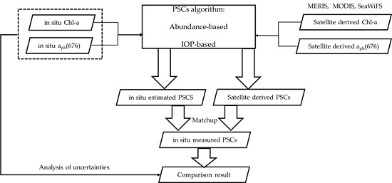
2. Materials and Methods

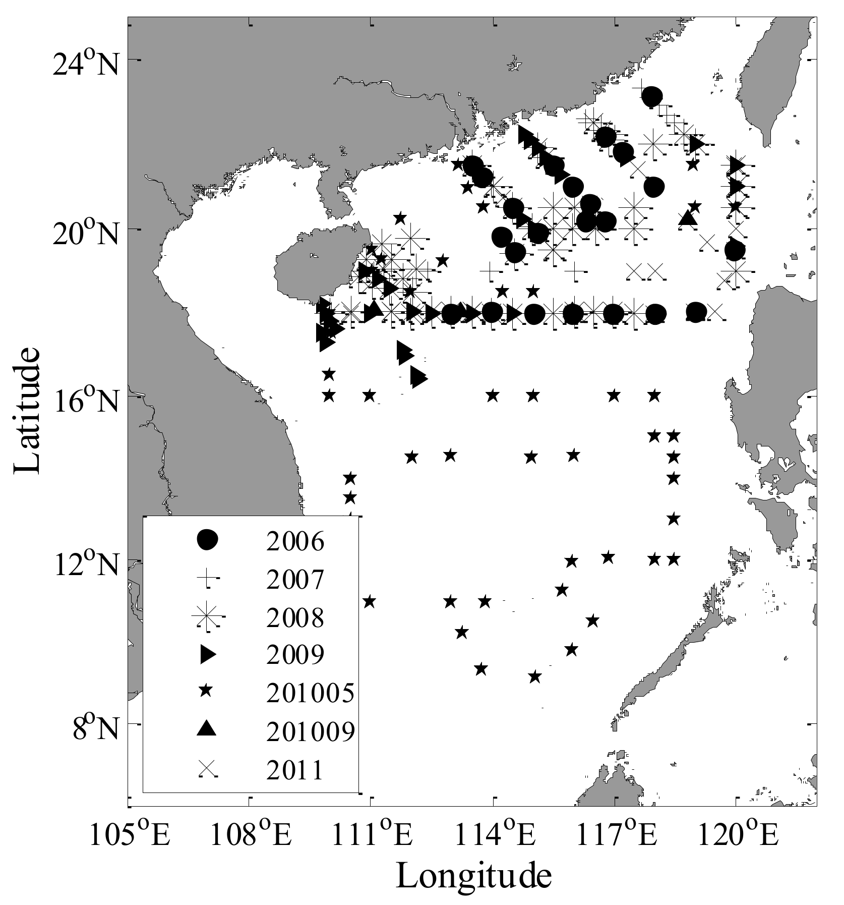
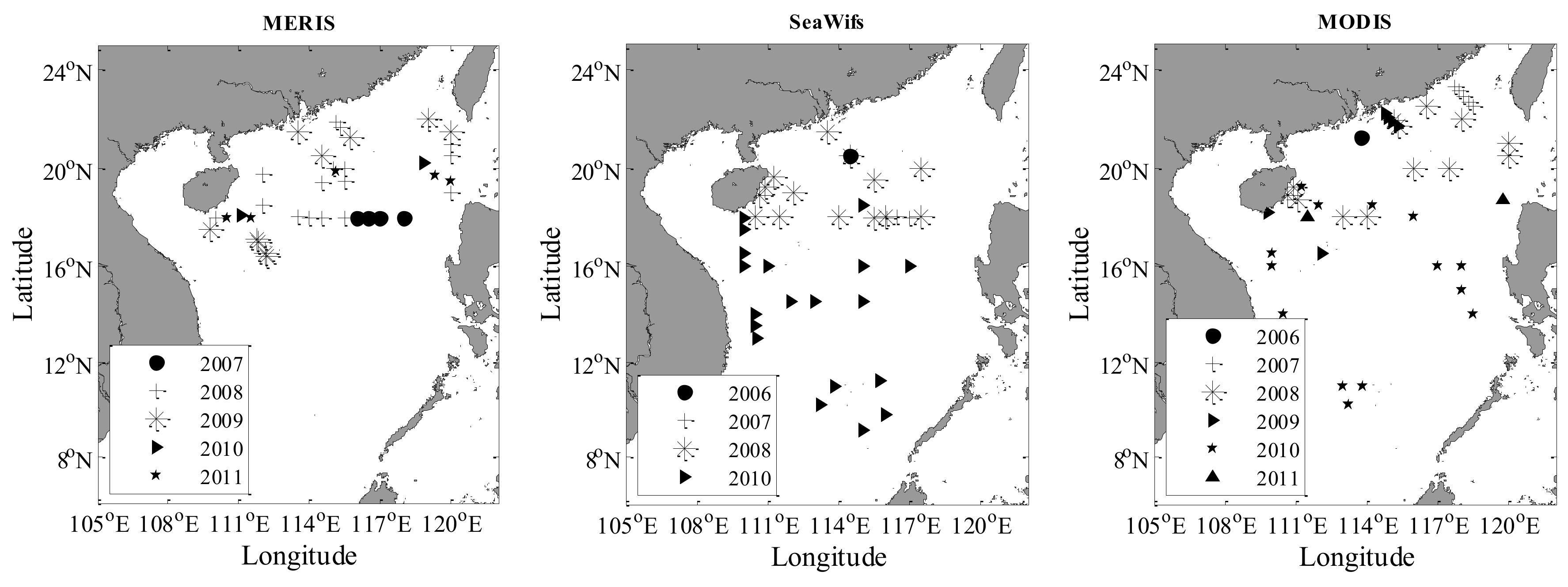
2.1. In-Situ Data

Field data were collected during a number of cruises in coastal and offshore waters from 2006 to 2011 (Figure 1). These cruises included the following: (1) six cruises in the Northern part of the South China Sea (NSCS) (August–September 2006, 2007, 2008, 2009, 2010 and 2011); and (2) one cruise in the SCS (April–May 2010). During each SCS and NSCS cruise, water samples from the surface were collected using Niskin bottles.

2.1.1. High Performance Liquid Chromatography Datasets

High Performance Liquid Chromatography (HPLC) pigment datasets were collected during SCS and NSCS cruises from 2006 to 2011, and they consisted of 410 measurements acquired from multiple locations which ensured high variability in phytoplankton pigments. Water samples (0.5–3 L) from certain depths were filtered onto a 25-mm glass fiber filter (Whatman GF/F). Following filtration, the samples were stored in liquid nitrogen. Fifteen pigments were quantified, and the diagnostic pigments include fucoxanthin, peridinin, 19′-hexanoyloxyfucoxanthin, 19′-butanoyloxyfucoxanthin, alloxanthin, chlorophyll-b and divinyl chlorophyll-b and zeaxanthin. Total chlorophyll a (Chl-a) is the sum of chlorophyll a, divinyl chlorophyll a and chlorophyllide a. Only the samples taken in the top 10 m of the water column were selected, and the quality assurance of pigment data was performed according to [24], ultimately yielding 233 surface HPLC samples. The fractions [F] of picoplankton (F_p), nanoplankton (F_n), and microplankton (F_m) were calculated from HPLC measurements using diagnostic pigment analysis (DPA) [5,25]. The fractions [F] of each size class can be inferred as

$$\mathrm{C}={\displaystyle \sum _{\mathrm{i}=1}^7{\mathrm{W}}_{\mathrm{i}}}{\mathrm{P}}_{\mathrm{i}}$$

(1)

$${\mathrm{F}}_{\mathrm{m}}=\frac{{\displaystyle \sum _{\mathrm{i}=1}^2{\mathrm{W}}_{\mathrm{i}}}{\mathrm{P}}_{\mathrm{i}}}{\mathrm{C}}$$

(2)

$${\mathrm{F}}_{\mathrm{n}}=\frac{{\displaystyle \sum _{\mathrm{i}=3}^5{\mathrm{W}}_{\mathrm{i}}}{\mathrm{P}}_{\mathrm{i}}}{\mathrm{C}}$$

(3)

$${\mathrm{F}}_{\mathrm{p}}=\frac{{\displaystyle \sum _{\mathrm{i}=6}^7{\mathrm{W}}_{\mathrm{i}}}{\mathrm{P}}_{\mathrm{i}}}{\mathrm{C}}$$

(4)

where [W] = {1.41; 1.41; 1.27; 0.35; 0.6; 1.01; 0.86} and [P] = {fucoxanthin; peridinin; 19′-hexanoyloxyfucoxanthin; 19′-butanoyloxyfucoxanthin; alloxanthin; chlorophyll-b and divinyl chlorophyll-b; zeaxanthin}. Note that 19′-hexanoyloxyfucoxanthin signal was probably attributable to pico-eukaryotes rather than to nanoplankton, and thus diagnostic pigment correction was performed according to [26], so that for C < 0.08, Equations (3) and (4) are adjusted as follows:

$${\mathrm{F}}_{\mathrm{n}}=\frac{12.5\mathrm{C}{\mathrm{W}}_3{\mathrm{P}}_3}{\mathrm{C}}+\frac{{\displaystyle \sum _{\mathrm{i}=4}^5{\mathrm{W}}_{\mathrm{i}}}{\mathrm{P}}_{\mathrm{i}}}{\mathrm{C}}$$

(5)

$${\mathrm{F}}_{\mathrm{p}}=\frac{(-12.5\mathrm{C}+1){\mathrm{W}}_3{\mathrm{P}}_3}{\mathrm{C}}+\frac{{\displaystyle \sum _{\mathrm{i}=6}^7{\mathrm{W}}_{\mathrm{i}}}{\mathrm{P}}_{\mathrm{i}}}{\mathrm{C}}$$

(6)

2.1.2. Spectral Absorption of Phytoplankton

For phytoplankton absorption measurements, water samples (0.5–3 L) from certain depths were filtered onto a 25-mm glass fiber filter (Whatman GF/F) at a low vacuum to record the particulate absorption measurements. Filters were kept in liquid nitrogen before analysis. In the laboratory, we measured the absorption spectra of the particles (a_p(λ)) using an ultraviolet-visible spectrophotometer (Shimadzu, UV-2550) equipped with an integrating sphere (T method, measuring the transmittance of a sample filter relative to a blank reference filter [27]). Spectra were acquired between 240 and 800 nm with a 1-nm step. Then, phytoplankton pigments were removed from the filter using a methanol treatment for 90–180 min [28]. The sample filter was rescanned to measure the non-algal absorption spectra (a_d(λ)) using the same method. The absorption spectra of a_ph(λ) were determined using the difference between a_p(λ) and a_d(λ). All spectra were shifted to zero in the near infrared region by subtracting the average optical density between 750 and 800 nm to minimize any possible differences between the sample and reference filters [29]. The path-length amplification effect was corrected in accordance with the method proposed by [30].

2.2. Satellite-Derived Data

2.2.1. Satellite Products

MODIS (Aqua), SeaWiFS, and MERIS (Reduced Resolution, RR) Level 2 (L2) data products were downloaded from NASA’s OceanColor website (http://oceancolor.gsfc.nasa.gov/). These data were processed by the l2gen operational software program (processing versions R2014.0, R2014.0, and R2012.1 for MODIS, SeaWiFS, and MERIS respectively). For SeaWiFS, Global Area Coverage (GAC, spatial resolution 4 km) data were used (Because data were available only for SeaWiFS GAC from 2007 to 2010 in the SCS). Previous studies have indicated minimal differences between the results of GAC and MLAC (Merged Local Area Coverage) retrieval products and in situ data in the SCS [22,23].

2.2.2. Matching Procedures for Satellite and In-Situ Data

To assess the performance of PSCs algorithms, satellite products were compared to the “matching” in-situ data. The HPLC data were matched to the closest spatial and temporal satellite pixel within a certain threshold. The first step was to find the closest 3 × 3 pixel window to the location of the in-situ measurement within a time interval of +/−48 h. Second, pixels from windows with poor quality, as defined by the quality control flags in the data products (i.e., problems due to clouds, stray light, glint, atmospheric correction failure, high top-of-atmosphere radiance, low water-leaving radiance, large solar/viewing angles, and navigation failure), were then discarded. Finally, if the percentage of remaining pixels in each window exceeded 50%, then the pixel window was accepted for subsequent matching analysis (for detailed matching procedures, refer to [31]). As a result, this criterion produced 48 in-situ and satellite data pairs for MODIS-Aqua, 41 pairs for MERIS, and 42 pairs for SeaWiFS GAC.

2.3. PSCs Algorithms

Algorithms designed to retrieve PSCs information from satellite data depend generally on either the spectral optical properties or the abundance of phytoplankton (Chl-a). IOP-based approaches rely on the covariation between spectral features of optical properties (absorption or backscattering) and PSCs [6,16,32]. Abundance-based approaches rely on the observed relationships between the trophic status of an environment and PSCs, on the premise that smaller cells are associated with oligotrophic conditions, whereas larger cells are associated with eutrophic conditions [10,12]. In this study, we incorporated four published PSCs satellite approaches designed for global applications using ocean colour sensors (

Table 1. Overview of the PSCs algorithms used in this study.

Algorithm Publication(s)	Acronym	Input Data	Methodology
Uitz et al., (2006)	Uitz2006	Chl-a, Ze, Zm	Abundance-based
Brewin et al., (2010)	Brewin2010	Chl-a	Abundance-based
Hirata et al., (2011)	Hirata2011	Chl-a	Abundance-based
Roy et al., (2011, 2013)	Roy2013	aph * (676)	IOP-based

Note: Chl-a is the concentration of chlorophyll-a; Z_e is the euphotic depth; Z_m is the mixed layer depth.

).

2.3.1. Abundance-Based PSCs Algorithm: Uitz2006

The Uitz2006 algorithm involves dividing global oceanic waters into stratified and mixed environments based on the ratio of the euphotic depth (Z_e) to the mixed layer depth (Z_m). Given information on the surface chlorophyll-a concentration, Z_e and Z_m, the percentage of the three phytoplankton size classes at a given pixel can be estimated. In this study, Z_e was inferred from a bio-optical model for light propagation [33]. Z_m was extracted for the appropriate month and geographic location from the published mixed layer depth climatology database (http://apdrc.soest.hawaii.edu /datadoc/mld.php). In order to be consistent with [5], the fractions [F] of each size class used here were calculated by Equations (1)–(4), and the specific parameters of PSCs algorithms were the same as those used in ref. [5].

2.3.2. Abundance-Based PSCs Algorithm: Brewin2010

The Brewin2010 algorithm describes the exponential functions that relate Chl-a to the fractional contribution of various PSCs. This model is based on the assumption that small cells dominate at low Chl-a concentrations and large cells at high Chl-a concentrations. In our study, the reparameterized three-component PSCs model using seven years of pigment measurements acquired in the SCS was selected. For comparison, parameter values from other oceans are also provided (

Table 2. Parameter values derived from fitting the three-component model to pigment data from the South China Sea. For comparison, parameter values from other oceans are also provided. ${\mathrm{C}}_{\mathrm{p},\mathrm{n}}^{\mathrm{m}}$ and ${\mathrm{C}}_{\mathrm{p}}^{\mathrm{m}}$ are the asymptotic maximum values for ${\mathrm{C}}_{\mathrm{p},\mathrm{n}}$ and ${\mathrm{C}}_{\mathrm{p}}$, respectively. S_p,n and S_p are the initial slopes.

Study Regions	${\mathbf{C}}_{\mathbf{p},\mathbf{n}}^{\mathbf{m}}$ (mg m−3)	Sp,n	${\mathbf{C}}_{\mathbf{p}}^{\mathbf{m}}$ (mg m−3)	Sp
South China Sea (this study) [4]	0.953	0.984	0.256	3.535
Atlantic Ocean [26]	0.977	0.910	0.095	7.822
Indian Ocean [34]	0.937	1.033	0.170	4.804
Global [35]	0.770	1.221	0.130	6.154

).

2.3.3. Abundance-Based PSCs Algorithm: Hirata2011

The Hirata2011 algorithm estimates fractions of three PSCs from empirical relationships between Chl-a and diagnostic pigments of various phytoplankton groups [14]. The model parameters are estimated using a large database (from various sources and different regions) of HPLC measurements. In order to be consistent with [14], the proportion of Fuco as a diatom biomarker is corrected (Fuco_corrected = Fuco_original − (Fuco/Hex)_baseline × Hex_original). (Fuco/Hex)_baseline was calculated using Fuco and Hex (data set from the SCS) in the Chl-a range less than 0.25 mg m^-3. After that, in situ PSCs were defined and classified as in the Brewin2010 algorithm. The estimated PSCs can be derived by the following equations (C is the concentration of Chl-a):

$${\mathrm{F}}_{\mathrm{m}}={[0.912+\mathrm{e}\mathrm{x}\mathrm{p}(-2.733{\log }_{10}(\mathrm{C}))+0.400]}^{-1}$$

(7)

$${\mathrm{F}}_{\mathrm{p}}=-{[0.153+\mathrm{e}\mathrm{x}\mathrm{p}(1.031\mathrm{l}\mathrm{o}{\mathrm{g}}_{10}(\mathrm{C})-1.558)]}^{-1}-1.086\mathrm{l}\mathrm{o}{\mathrm{g}}_{10}(\mathrm{C})+2.995$$

(8)

$${\mathrm{F}}_{\mathrm{n}}=1-{\mathrm{F}}_{\mathrm{m}}-{\mathrm{F}}_{\mathrm{p}}$$

(9)

2.3.4. IOP-Based PSCs Algorithm: Roy2013

The Roy2013 algorithm utilizes phytoplankton absorption at 676 nm to derive the power-law exponent/slope of the phytoplankton size spectrum (ξ). The method relies on measurements of two quantities of a phytoplankton sample: Chl-a and a_ph(676) [16]. In this study, the Chl-a products of MERIS, MODIS and SeaWiFS were obtained using the OC4 empirical maximum band ratio algorithm. For satellite derived a_ph(676), two existing IOPs algorithms were applied to assess its performance in the SCS: (1) the Garver–Siegel–Maritorena (GSM) model [36]; and (2) the default global configuration of the Generalized Inherent Optical Property (GIOP) model [37]. The proportions of Chl-a within any diameter range of PSCs can be calculated as follows:

$${\mathrm{F}}_{\mathrm{p}}=\frac{{\mathrm{D}}_1^{4-\mathsf{\xi }-\mathrm{m}}-{\mathrm{D}}_0^{4-\mathsf{\xi }-\mathrm{m}}}{{\mathrm{D}}_3^{4-\mathsf{\xi }-\mathrm{m}}-{\mathrm{D}}_0^{4-\mathsf{\xi }-\mathrm{m}}}$$

(10)

$${\mathrm{F}}_{\mathrm{n}}=\frac{{\mathrm{D}}_2^{4-\mathsf{\xi }-\mathrm{m}}-{\mathrm{D}}_1^{4-\mathsf{\xi }-\mathrm{m}}}{{\mathrm{D}}_3^{4-\mathsf{\xi }-\mathrm{m}}-{\mathrm{D}}_0^{4-\mathsf{\xi }-\mathrm{m}}}$$

(11)

$${\mathrm{F}}_{\mathrm{p}}=\frac{{\mathrm{D}}_3^{4-\mathsf{\xi }-\mathrm{m}}-{\mathrm{D}}_2^{4-\mathsf{\xi }-\mathrm{m}}}{{\mathrm{D}}_3^{4-\mathsf{\xi }-\mathrm{m}}-{\mathrm{D}}_0^{4-\mathsf{\xi }-\mathrm{m}}}$$

(12)

where m = 0.06 (dimensionless), D is the cell diameter, D₀ = 0.2 μm, D₁ = 2 μm, D₂ = 20 μm, and D₃ = 50 μm. as ξ→ (4-m); the above fractions can be approximated as:

$${\mathrm{F}}_{\mathrm{p}}=\frac{{\log }_{\mathrm{e}}({\mathrm{D}}_1/{\mathrm{D}}_0)}{{\log }_{\mathrm{e}}({\mathrm{D}}_3/{\mathrm{D}}_0)}$$

(13)

$${\mathrm{F}}_{\mathrm{n}}=\frac{{\log }_{\mathrm{e}}({\mathrm{D}}_2/{\mathrm{D}}_1)}{{\log }_{\mathrm{e}}({\mathrm{D}}_3/{\mathrm{D}}_0)}$$

(14)

$${\mathrm{F}}_{\mathrm{m}}=\frac{{\log }_{\mathrm{e}}({\mathrm{D}}_3/{\mathrm{D}}_2)}{{\log }_{\mathrm{e}}({\mathrm{D}}_3/{\mathrm{D}}_0)}$$

(15)

2.4. Statistical Methods

Several statistical parameters (Equations (16)–(18)) were used to evaluate the matching comparison results: (1) MR, the median of the ratio of satellite-derived values to in-situ values, provided a measure of overall bias for the comparison; (2) SIQR, the semi-interquartile range calculated for the satellite to in-situ ratio, indicated the spread of these data; and (3) RMSE, the relative root mean squared error, was used to assess the uncertainty.

$$\mathrm{M}\mathrm{R}=\mathrm{m}\mathrm{e}\mathrm{d}\mathrm{i}\mathrm{a}\mathrm{n}(\frac{{\mathrm{y}}_{\mathrm{i}}}{{\mathrm{x}}_{\mathrm{i}}})$$

(16)

$$\mathrm{S}\mathrm{I}\mathrm{Q}\mathrm{R}=\frac{({\mathrm{Q}}_3-{\mathrm{Q}}_1)}{2}$$

(17)

$$\mathrm{R}\mathrm{M}\mathrm{S}\mathrm{E}(\%)=100\times {\left\{\frac{1}{\mathrm{N}}{\displaystyle \sum _{\mathrm{i}=1}^{\mathrm{N}}{[\frac{{\log }_{10}{\mathrm{x}}_{\mathrm{i}}-{\log }_{10}{\mathrm{y}}_{\mathrm{i}}}{{\log }_{10}{\mathrm{x}}_{\mathrm{i}}}]}^2}\right\}}^{1/2}$$

(18)

where y_i is the satellite-retrieved value, x_i is the in-situ value, and N is the number of matching data points. Q₁ is the 25th percentile and Q₃ the 75th percentile. A least-squares fit was also performed within the matching points (performed in log₁₀ space), giving the associated coefficient of determination (R²) and slope S.

3. Results

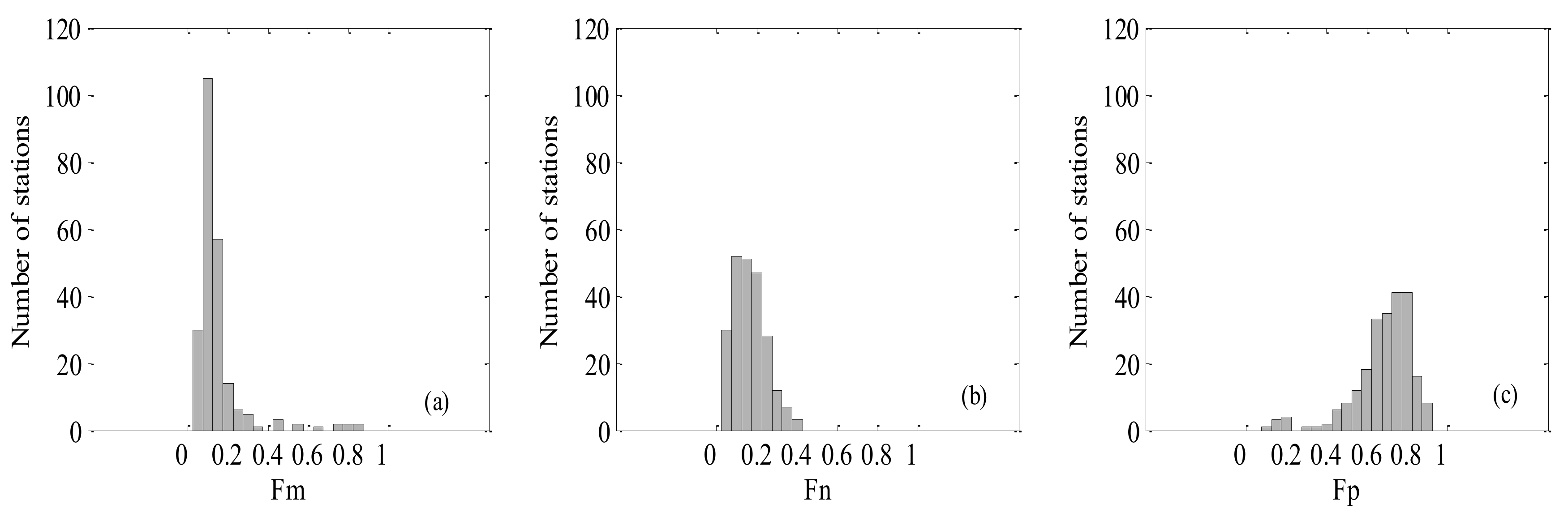
3.1. Statistics of In Situ Datasets and Match-up Data

Figure 1 and Figure 2 show the spatial distribution of in situ HPLC measurement and the valid matches for MERIS, MODIS, and SeaWiFS. The in situ and matched values exhibited a range of spatial variation. The fraction of picoplankton varied from 0.1 to 0.9 (average 0.71) and was dominant in the open ocean. High proportions of microphytoplankton and nanophytoplankton were found over the coastal regions. The specific statistics are shown in Figure 3 and

Table 3. Statistics of in situ and matched HPLC datasets. SD, max and min represent the standard deviation, maximum, and minimum values, respectively. The units for Chl-a are mg m⁻³, N is the number of samples. * denotes valid matches for MERIS, MODIS, and SeaWiFS.

In Situ Data	Median ± SD	Average	Max.	Min.	N
Fm	0.12 ± 0.14	0.16	0.85	0.05	230
Fn	0.17 ± 0.09	0.16	0.40	0.03	230
Fp	0.71 ± 0.15	0.68	0.91	0.09	230
Chl-a	0.10 ± 0.43	0.20	3.25	0.03	230
Fm *	0.12 ± 0.15	0.17	0.83	0.05	101
Fn *	0.15 ± 0.08	0.16	0.39	0.03	101
Fp *	0.74 ± 0.16	0.70	0.91	0.13	101

Note: F_m, F_n and F_p is the fractions of picoplankton (<2 μm), nanoplankton (2–20 μm), and microplankton (>20 μm).

. For matchups (include MERIS, MODIS, and SeaWiFS), the corresponding statistical results were similar to the HPLC data sets, suggesting that these matchups can give typical and representative validation in the SCS.

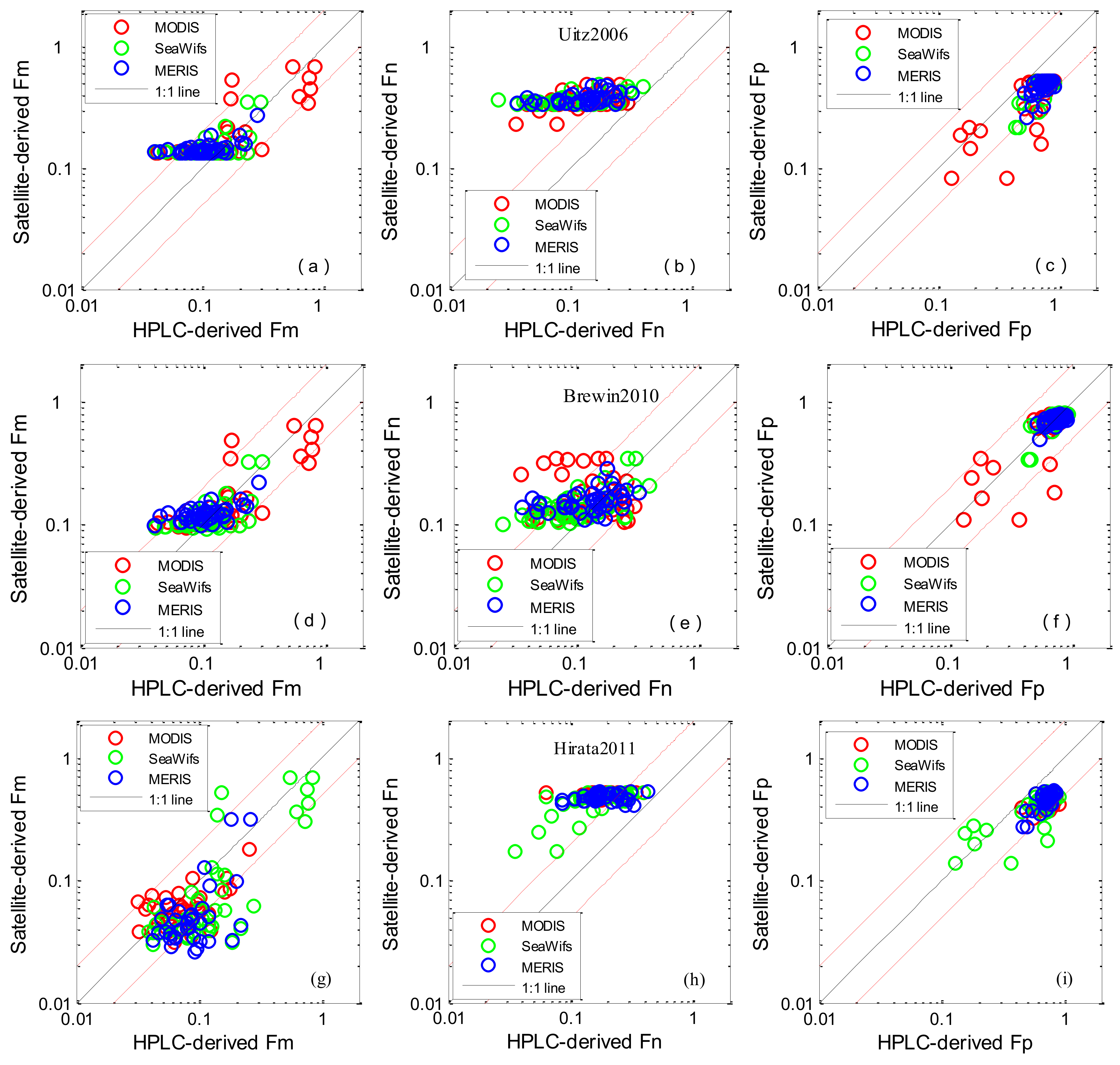
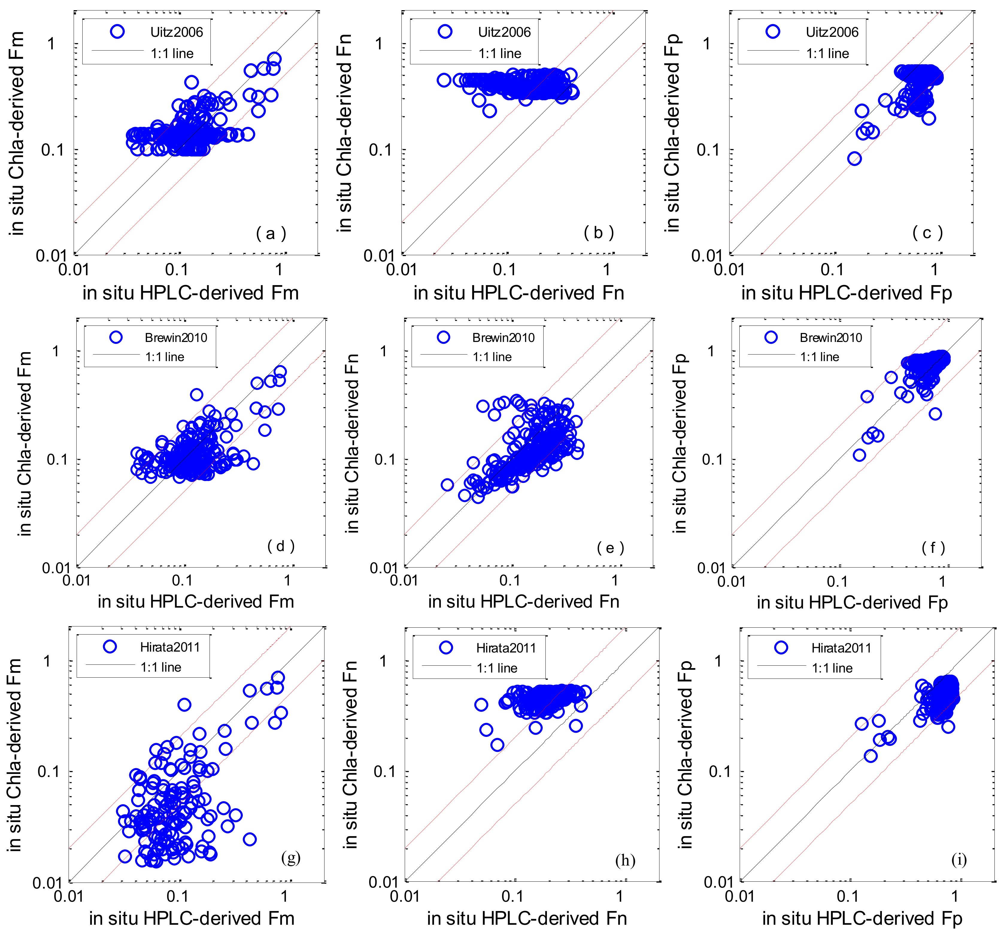
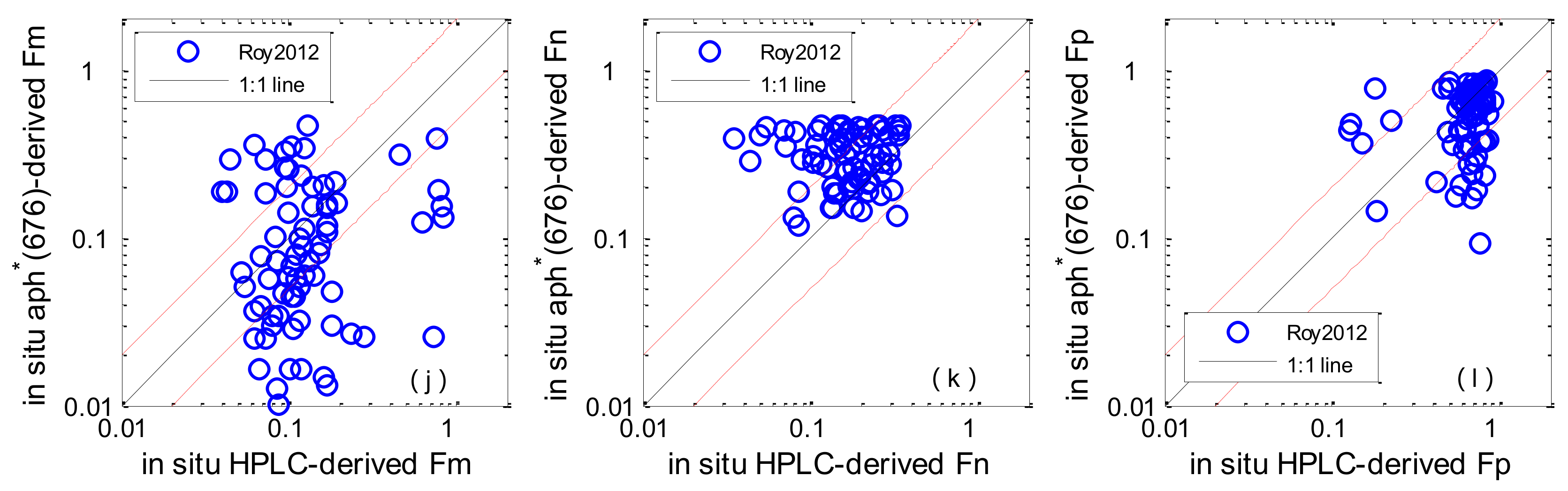
3.2. Algorithm Evaluation Using In-Situ Data

Figure 4a–l shows the performances of different algorithms when in situ Chl-a and a_ph * (676) were used as the algorithm inputs. The statistical results of MR, SIQR and RMSE are shown in

Table 4. Statistical results for the validation of the selected algorithms using in-situ data. The slope is the linear regression results from retrieval values versus in situ ones. N is the number of samples.

Algorithm	MR	SIQR	RMSE (%)	R2	Slope	N
Fm
Uitz2006	1.204	0.298	32.666	0.307	0.504	227
Brewin2010	0.906	0.246	38.848	0.292	0.487	227
Hirata2011	0.612	0.339	71.525	0.205	0.599	178
Roy2013	0.589	0.464	221.282	0.011	0.065	75
Fn
Uitz2006	2.421	1.005	49.956	0.039	−0.078	227
Brewin2010	0.778	0.187	32.090	0.355	0.368	227
Hirata2011	2.243	0.500	51.346	0.171	0.356	178
Roy2013	1.675	0.676	40.215	0.000	0.083	75
Fp
Uitz2006	0.647	0.081	205.294	0.418	0.332	227
Brewin2010	1.068	0.069	44.566	0.597	0.715	227
Hirata2011	0.709	0.102	148.755	0.481	0.433	178
Roy2013	0.854	0.253	238.369	0.008	0.254	75

. Concerning picoplankton, Brewin2010 performed with the highest accuracy, with a median bias of 6.8% (MR = 1.068) and the RMSE was 44.5%; Uitz2006 and Hirata2011 slightly underestimated values at the higher end of measured F_p, with median biases of −35.3% and −28.1%, and RMSEs of 205.3% and 148.8% respectively. Concerning microplankton, Uitz2006 and Brewin2010 performed with higher accuracy—the RMSEs for the F_m were 32.7% and 38.8% and the MR were 1.20 and 0.91, respectively; Hirata2011 underestimated F_m when the fractions were low, with a median bias of −39% (MR = 0.61). The detection of nanoplankton was generally worse than those of microplankton and picoplankton, Brewin2010 showed the best performance (F_n) among all algorithms.

With regard to the a_ph * (676)-based algorithm, Roy2013 showed the worst performance regarding F_m and F_p with RMSE of 221.8% and 238.4%. However, Roy2013 performed better than Uitz2006 and Hirata2011 at detecting F_n.

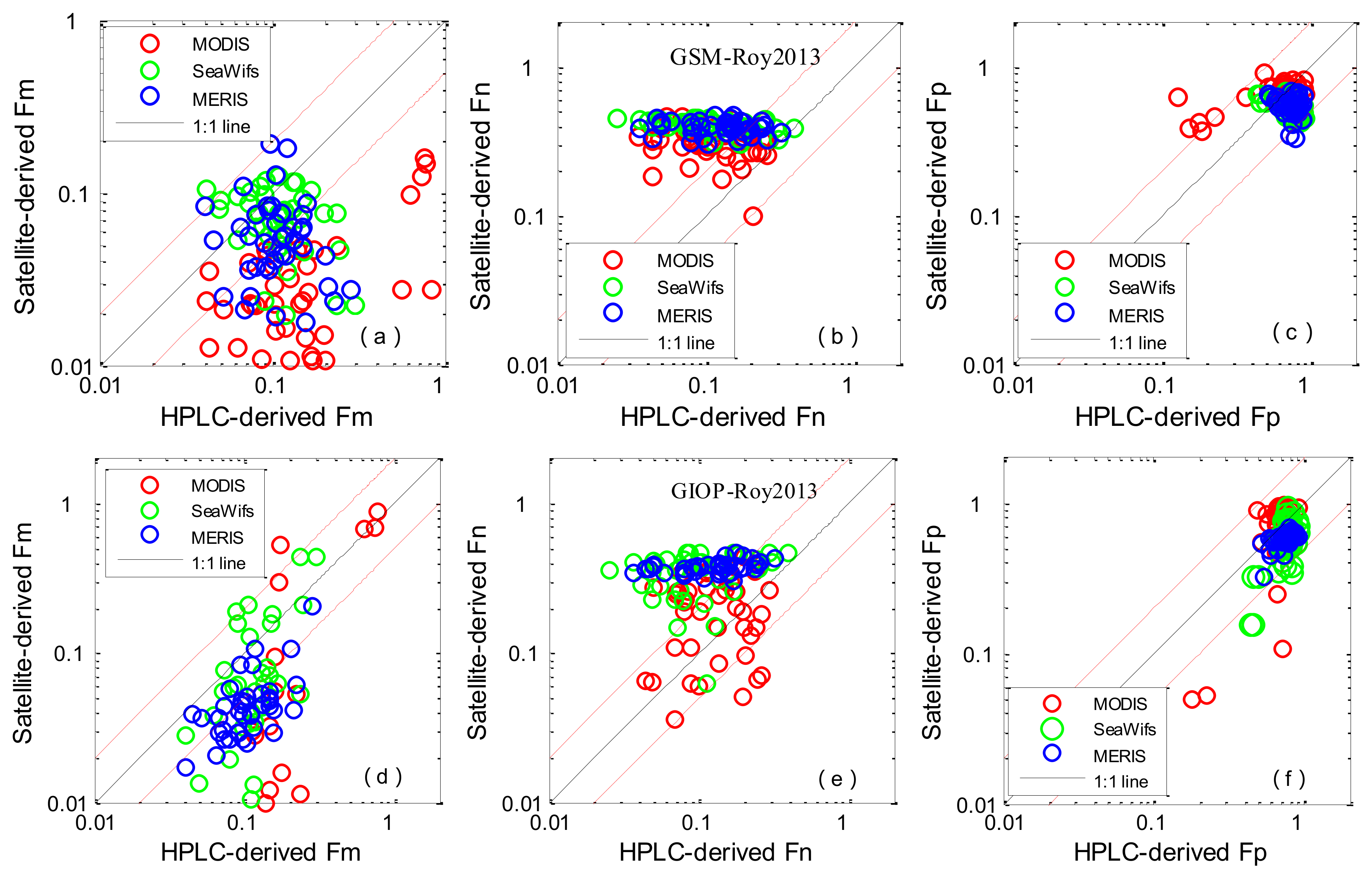
3.3. Algorithm Evaluation Using Satellite Data

All algorithms were applied to the ocean colour satellite products of MODIS, SeaWiFS and MERIS, and the derived values were compared with the in situ HPLC data (Figure 5 and Figure 6). The statistical results are shown in

Table 5. Statistical results for the validation of abundance-based algorithms for MERIS, MODIS and SeaWiFS. The slope is the linear regression results from retrievals versus in situ ones. N is the number of samples.

Algorithm	MR	SIQR	RMSE	R2	Slope	N
Fm
Uitz2006MODIS	1.218	0.396	59.382	0.584	0.584	48
Uitz2006Meris	1.362	0.314	18.091	0.304	0.331	41
Uitz2006Seawifs	1.258	0.248	18.696	0.288	0.572	42
Uitz2006Average	1.275	0.333	38.814	0.504	0.579	131
Brewin2010MODIS	0.965	0.277	68.146	0.624	0.563	48
Brewin2010Meris	1.170	0.248	15.408	0.325	0.294	41
Brewin2010Seawifs	1.055	0.223	16.878	0.357	0.605	42
Brewin2010Average	1.042	0.268	43.211	0.536	0.558	131
Hirata2011MODIS	0.631	0.255	70.907	0.591	0.673	48
Hirata2011Meris	0.808	0.214	21.581	0.274	0.383	41
Hirata2011Seawifs	0.599	0.255	35.700	0.184	0.663	42
Hirata2011Average	0.697	0.252	48.955	0.421	0.666	131
Fn
Uitz2006MODIS	2.983	1.281	51.083	0.198	0.276	48
Uitz2006Meris	2.612	0.904	51.448	0.183	0.272	41
Uitz2006Seawifs	3.759	1.408	54.118	0.237	0.299	42
Uitz2006Average	3.028	1.256	52.188	0.197	0.286	131
Brewin2010MODIS	1.417	0.609	32.511	0.000	−0.050	48
Brewin2010Meris	1.105	0.441	22.535	0.122	0.182	41
Brewin2010Seawifs	1.373	0.538	26.131	0.347	0.406	42
Brewin2010Average	1.306	0.524	27.661	0.083	0.199	131
Hirata2011MODIS	2.715	0.788	55.639	0.447	0.602	48
Hirata2011Meris	2.685	0.320	58.472	0.043	0.092	41
Hirata2011Seawifs	2.897	0.527	55.838	0.024	0.054	42
Hirata2011Average	2.755	0.497	56.604	0.287	0.336	131
Fp
Uitz2006MODIS	0.668	0.075	216.880	0.608	0.536	48
Uitz2006Meris	0.646	0.033	212.641	0.401	0.416	41
Uitz2006Seawifs	0.648	0.052	253.765	0.639	0.532	42
Uitz2006Average	0.650	0.051	228.107	0.617	0.519	131
Brewin2010MODIS	0.980	0.117	81.580	0.612	0.810	48
Brewin2010Meris	0.951	0.053	56.528	0.396	0.354	41
Brewin2010Seawifs	0.949	0.071	52.072	0.613	0.686	42
Brewin2010Average	0.967	0.068	65.635	0.623	0.736	131
Hirata2011MODIS	0.650	0.077	190.522	0.600	0.414	48
Hirata2011Meris	0.592	0.034	218.544	0.277	0.231	41
Hirata2011Seawifs	0.628	0.039	169.353	0.584	0.492	42
Hirata2011Average	0.619	0.049	193.504	0.579	0.401	131

^Average The average values of MODIS, SeaWiFS and MERIS.

and

Table 6. Statistical results for the validation of the inherent optical property (IOP)-based algorithm for MERIS, MODIS and SeaWiFS. The slope is the linear regression results from retrievals versus in situ ones. N is the number of samples.

Algorithm	MR	SIQR	RMSE	R2	Slope	N
Fm
a Roy2013MODIS	4.804	1.507	100.427	0.225	−0.272	48
a Roy2013MERIS	4.982	1.426	72.642	0.014	0.321	41
a Roy2013SeaWiFS	4.882	1.067	69.773	0.143	0.492	42
a Roy2013Average	4.964	1.408	83.114	0.000	−0.068	131
b Roy2013MODIS	5.567	2.564	334.090	0.520	−1.189	41
b Roy2013MERIS	5.601	1.558	74.534	0.342	−0.842	39
b Roy2013SeaWiFS	5.278	1.683	73.616	0.249	−1.577	39
b Roy2013Average	5.567	2.065	205.068	0.361	−0.984	119
Fn
a Roy2013MODIS	2.705	1.585	47.053	0.041	−0.227	48
a Roy2013MERIS	2.864	1.055	53.279	0.010	−0.084	41
a Roy2013SeaWiFS	4.341	1.898	58.924	0.217	−0.210	42
a Roy2013Average	3.076	1.669	53.036	0.040	−0.196	131
b Roy2013M°DIS	1.506	0.852	42.041	0.025	0.166	41
b Roy2013MERIS	2.719	1.087	51.524	0.155	0.238	39
b Roy2013SeaWiFS	3.568	1.701	53.018	0.028	0.372	39
b Roy2013Average	2.496	1.185	48.992	0.004	0.195	119
Fp
a Roy2013MODIS	0.032	0.019	1666.956	0.142	−0.108	48
a Roy2013MERIS	0.072	0.023	1211.414	0.053	0.077	41
a Roy2013SeaWiFS	0.092	0.023	1198.100	0.266	0.122	42
a Roy2013Average	0.066	0.033	1392.007	0.000	−0.008	131
b Roy2013MODIS	0.006	0.012	2934.519	0.274	−0.955	41
b Roy2013MERIS	0.056	0.017	1360.411	0.425	−0.207	39
b Roy2013SeaWiFS	0.068	0.046	1924.974	0.206	−0.670	39
b Roy2013Average	0.042	0.036	2188.129	0.099	−0.724	119

^a The combined model, GIOP-Roy2013; ^b The combined model, GSM-Roy2013. ^Average The average values of MODIS, SeaWiFS and MERIS.

. When comparing the results from the four methods listed in Table 1, it firstly appears that abundance-based algorithms performed with higher accuracy than the IOP-based method. For abundance-based algorithms, the evaluation results using in situ and satellite-derived Chl-a showed good tendency towards accuracy. Concerning picoplankton, Brewin2010 performed with the highest accuracy—the median biases of the three satellites were −0.02%, −0.51% and −0.49% for MODIS, SeaWiFS and MERIS, respectively, the RMSEs were 81.6%, 52.1%, and 56.5% and the coefficients of determination were 0.61, 0.61, and 0.40, respectively. For Uitz2006 and Hirata2011, underestimation of the satellite-derived F_p was observed—the average median satellite/in situ ratios were 0.65 and 0.70. Concerning microplankton, Uitz2006 and Brewin2010 were found to perform with higher accuracy—the median biases of the three satellites were 21.8%/−3.5%, 36.2%/17.0% and 25.8%/5.5% for MODIS, SeaWiFS and MERIS, respectively and the RMSEs were 59.4%/68.0%, 18.1%/15.4%, and 18.7%/16.9%; Hirata2011 underestimated the measured F_m when the concentration of microplankton was low, with median biases of −37.0%, −20.0% and −40.1%, and RMSEs were 70.9%, 21.4% and 35.7% for MODIS, SeaWiFS and MERIS, respectively. Concerning nanoplankton, Uitz2006 and Hirata2011 were found to have bad performances, the average RMSEs were 52.1% and 56.6%. With regard to the a_ph * (λ)-based PSCs algorithm, the performances of GIOP-Roy2013 and GSM-Roy2013 are shown in Figure 6, and the corresponding statistical results are provided in Table 6. GIOP-Roy2013 performed with higher accuracy for detecting microplankton than GSM-Roy2013, especially when F_m was high. Concerning picoplankton, when F_p < 0.5, GSM-Roy2013/GIOP-Roy2013 showed an overestimation/underestimation. MODIS derived F_n (GIOP-Roy2013) seemed to have higher accuracy than MERIS and SeaWiFs.

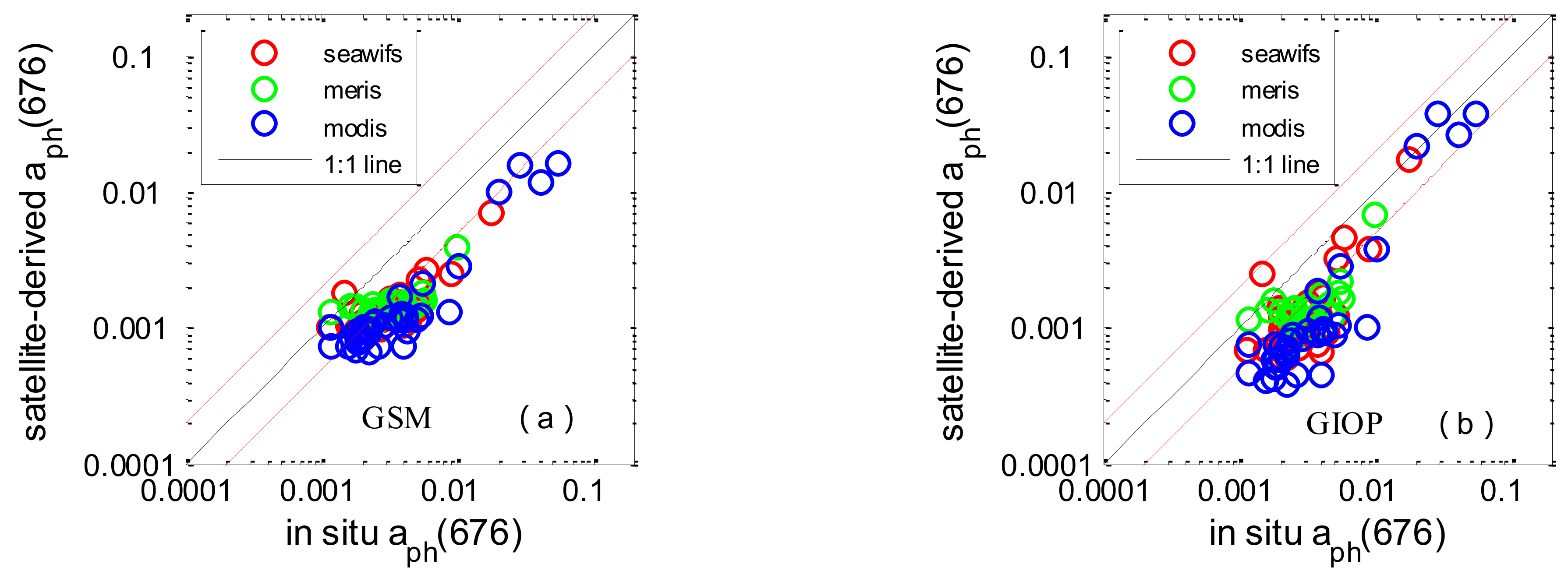
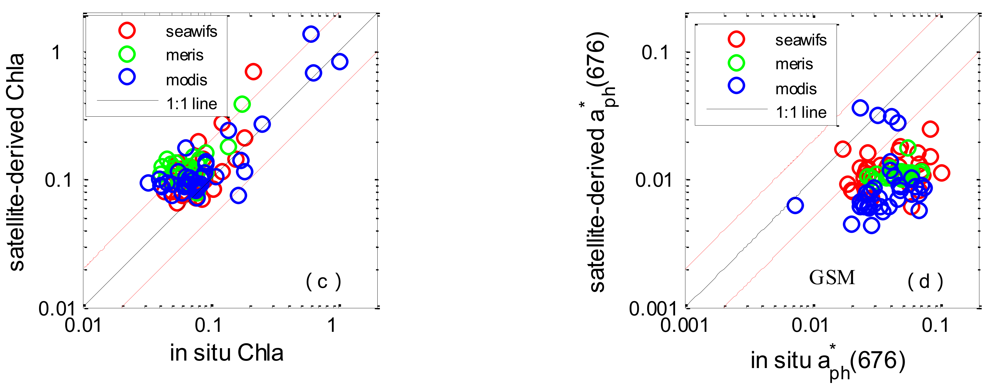
3.4. Chl-a and a_ph(676) Assessment in the SCS

The comparison statistics associated with Chl-a and a_ph(676) are shown in

Table 7. Statistical results for the validation of abundance-based algorithms for MERIS, MODIS and SeaWiFS. The slope is the linear regression results from retrievals versus in situ ones. N is the number of samples.

Name	MR	SIQR	RMSE	R2	Slope	N
a aph(676)MODIS	0.403	0.084	20.785	0.858	0.334	37
a aph(676)MERIS	0.485	0.096	15.168	0.475	0.242	21
a aph(676)SeaWiFS	0.443	0.096	16.920	0.672	0.299	37
a aph(676)Average	0.434	0.104	18.183	0.745	0.328	95
b aph(676)MODIS	0.306	0.064	22.423	0.858	0.800	37
b aph(676)MERIS	0.448	0.104	15.152	0.453	0.513	21
b aph(676)SeaWiFS	0.430	0.077	17.593	0.617	0.797	37
b aph(676)Average	0.376	0.097	19.161	0.723	0.795	95
Chl-aMODIS	1.305	0.228	38.896	0.785	0.556	37
Chl-aMERIS	1.834	0.308	26.108	0.472	1.546	21
Chl-aSeaWiFS	1.224	0.258	20.114	0.496	1.745	37
Chl-aAverage	1.429	0.373	24.713	0.643	0.573	95
a * ph(676)MODIS	0.265	0.084	44.495	0.038	0.016	37
a * ph(676)MERIS	0.257	0.042	48.389	0.007	−0.006	21
a * ph(676)SeaWiFS	0.339	0.157	43.918	0.027	−0.009	37
a * ph(676)Average	0.265	0.103	45.165	0.004	0.005	95

^a The combined model, GIOP-Roy2013; ^b The combined model, GSM-Roy2013. ^Average The average values of MODIS, SeaWiFS and MERIS.

. The Chl-a concentrations derived from SeaWiFS, MODIS, and MERIS data were lightly overestimated, with average satellite/in situ ratios of 1.22, 1.31, and 1.83, respectively. The RMSEs were 20.1%, 38.9%, and 26.1%. The average coefficients of determination were 0.64. Two IOP algorithms (GSM and GIOP) were used to derive the absorption coefficient of phytoplankton, and the results clearly showed that they underestimated the measured a_ph(676). The assessment showed a similar tendency towards accuracy between GSM and GIOP derived a_ph(676). Underestimation of a_ph(676) and the slight overestimation of Chl-a could lead to an underestimation of a * _ph(676), which is the input of Roy2013 (see in Figure 7). As for a * _ph(676), the validation result exhibited dispersion and poor statistical correlation, the average RMSEs for SeaWiFS, MODIS, and MERIS were 43.9%, 44.5% and 48.3% and the R² values were 0.03, 0.04 and 0.007.

4. Discussion

In this study, MERIS, MODIS, and SeaWiFS PSCs products for SCS were compared with in situ data collected from 2007 to 2011. Our purpose here was to inter-compare the performances of different PSCs algorithms. This work can aid in selecting the proper satellite PSCs model to best fit the required application in the SCS.

There are two main reasons for a mismatch between in situ-measured and satellite derived PCSs. The first is the possible uncertainty of satellite-derived phytoplankton abundance data (Chl-a) and IOP data and the second is the choice of PSCs algorithms. For the abundance-based algorithms, the comparison results of Chl-a generally showed reasonable agreement in the SCS (RMSE < 38% for all three satellites, Table 7); this is why the evaluation results using in situ and satellite-derived Chl-a showed a good tendency towards accuracy. Regarding the algorithms themselves, three of the abundance-based approaches presented above were designed to estimate fractions of size classes in a given Chl-a concentration. The Uitz2006 method assigns size classes according to a finite number of trophic status defined on the basis of surface Chl-a and on whether or not the euphotic zone may be treated as stratified or mixed [5]. The Brewin2010 and Hirata2011 methods are both based only on the Chl-a concentration but differ from each other in the functional relationships assigned to relate total Chl-a to size classes [10,12]. The performance of reparameterized Brewin2010 using seven years of pigment measurements acquired in the SCS is in agreement with the results of [26,34]. Regarding Uitz2006, comparison results of satellite derived F_m in the SCS is consistent with [5] which resulted from numerous field campaigns; while the derived F_p showed an obvious underestimation (but has good tendency towards accuracy). With regard to Hirata2011, both F_m and F_p were underestimated relative to previous results (which are based on a dataset from oceans around the world) [14]. The observed different performance compared with other areas indicated that the choice of a proper PSCs algorithm seems to be critical. It should be noted that Uitz2006 and Hirata2011 were originally not designed for coastal and shelf waters; this difference may impact the algorithm’s performance in the SCS (especially for water depth < 200 m). In addition, the observed different performances of the three abundance-based algorithms are likely related to different pigment-to-size methods (DPA). With regard to Brewin2010, part of the matched data for satellite validation (less than 1/5) was used to re-tune the algorithm; this could be helpful for the comparison result. For our regional application, it is better to reparameterize using the HPLC measurements collected in the SCS [4]. Regarding the a * _ph(λ)-based Roy2013 algorithm, the total absorption coefficient of phytoplankton in the red peak at 676 nm estimated from satellite remote sensing was used to compute the exponent of an assumed power-law (ξ) for phytoplankton particle size spectrum. Two IOP algorithms (GSM and GIOP) were used to derive the absorption coefficient of phytoplankton, and the results clearly show that they underestimated the measured a_ph(676). This means the development of robust IOP algorithms is still a challenge in the SCS. As for the algorithm itself, the validation result using in situ a * _ph(676) exhibited dispersion and poor statistical correlation (see in Figure 4), which implies much effort is needed to improve the quantitative information on phytoplankton size structure, namely, the exponent ξ of phytoplankton size spectrum and the equivalent spherical diameter of the population.

Other factors can confound comparison (between in situ and satellite) results. Firstly, there are measurement errors. An inter-comparison of HPLC pigment methods indicates an instrument error of 7% for total Chl-a and, on average, 21.5% for other pigments (ranging from 11.5% for fucoxanthin to 32.5% for peridinin), and an inverse dependence on pigment concentration (with large disagreements for pigments close to the detection limits) [38]. Secondly, there are uncertainties associated with the use of pigment concentration to determine size class. The HPLC DPA does not strictly reflect the true size of phytoplankton, and some taxonomic pigments might be shared by various phytoplankton groups. Different diagnostic pigment methods can bring deviations in the comparison result [5,13,17]. In addition, multiple regression analysis of Chl-a and the concentration of accessory pigments collected from the SCS need to be strengthened. Thirdly, the in situ observation was performed at a single location, while the minimum satellite resolution is about 1 × 1 km, and thus, spatial mismatch exists between in situ and satellite values. When ocean waters are patchy, for example, in eddies, fronts or river plumes, the two observational scales may eventually affect data comparison [13,39].

The detection of microplankton and picoplankton was generally better than that of nanoplankton in the SCS. This result was consistent with previous studies. This may be because of higher diversity in nanoplankton than pico- or microplankton, which may result in greater variability in their optical characteristics, making them harder to detect from satellite/in situ measurement [13]. It is worth noting that some of the results from the statistical analysis of satellite derived PSCs were slightly better than those obtained from only using in situ data (e.g., F_p- Brewin2010^Meris, F_m-Uitz2006^Seawifs). This abnormality might be partly explained by the differences in the dynamic range of the measured data or because there was not enough matching data.

Throughout the inter-comparisons of the four algorithms, we found that the abundance-based approaches provided better spatial retrieval of PSCs than IOP-based ones. Though abundance-based approaches are easy to implement and offer a simple and effective method for revealing the expected size structure of phytoplankton, they are indirect methods for detecting PSCs. They rely on observed patterns of change in the size structure with a change in the concentration of Chl-a. Variability in the optical properties of phytoplankton (e.g., changes in temperature, nutrient, species and light regimes) can make the algorithms less suitable for long-term analysis as this will require on-going comparison with in situ measurements [12,17]. Regarding IOP-based approaches, they are more direct and capable of detecting changes in size structure independent of phytoplankton concentration. However, accurately exploiting the optical characteristics (e.g., a_ph(676), b_bp(λ)) of different PSCs to build algorithms may not always be effective [12]. Further efforts to develop robust IOP algorithms and IOP-based PSCs algorithms are desirable in the SCS. The three-component model is recommended for use in the proposed procedure using satellite data to produce maps of surface PSCs in the SCS.

5. Conclusions

Four algorithms designed to detect phytoplankton size structure were assessed using in situ data and satellite data (MERIS, MODIS, SeaWiFS) in this study. Results indicated that, abundance-based approaches performed with better accuracy than optics-based ones, and the detection of microplankton and picoplankton were generally better than that of nanoplankton in the SCS. For the abundance-based algorithms, the selection of the PSCs algorithm seemed to be more critical to the performance of ocean colour data. For the IOP-based PSCs algorithms, the selection of a proper inherent optical property model and PSCs algorithm both had an impact on the satellite-derived results. The good performance of satellite derived a_ph(676) implies a potential for IOP-based PSCs algorithms in the SCS. Our comparison activity in the SCS advocated that (1) the three-component model is recommended for use for the proposed procedure using satellite data for application in the SCS; (2) developing robust IOP algorithms and optics-based PSCs algorithms is desirable; and (3) continuous support of dedicated to in-situ data collection is needed for validation purposes.

References

1. Falkowski, P.G.; Barber, R.T.; Smetacek, V. Biogeochemical controls and feedbacks on ocean primary production. Science 1998, 281, 200–206. [Google Scholar] [CrossRef] [PubMed]
2. Field, C.B.; Behrenfeld, M.J.; Randerson, J.T.; Falkowski, P. Primary production of the biosphere: Integrating terrestrial and oceanic components. Science 1998, 281, 237–240. [Google Scholar] [CrossRef] [PubMed]
3. Siegel, D.A.; Buesseler, K.O.; Doney, S.C.; Sailley, S.F.; Behrenfeld, M.J.; Boyd, P.W. Global assessment of ocean carbon export by combining satellite observations and food-web models. Glob. Biogeochem. Cycles 2014, 28, 181–196. [Google Scholar] [CrossRef]
4. Lin, J.; Cao, W.; Wang, G.; Hu, S. Satellite-observed variability of phytoplankton size classes associated with a cold eddy in the South China Sea. Mar. Pollut. Bull. 2014, 83, 190–197. [Google Scholar] [CrossRef] [PubMed]
5. Uitz, J.; Claustre, H.; Morel, A.; Hooker, S.B. Vertical distribution of phytoplankton communities in open ocean: An assessment based on surface chlorophyll. J. Geophys. Res. Ocean. 2006, 111, 275–303. [Google Scholar] [CrossRef]
6. Kostadinov, T.S.; Siegel, D.A.; Maritorena, S. Global variability of phytoplankton functional types from space: Assessment via the particle size distribution. Biogeosci. Discuss. 2010, 7, 3239–3257. [Google Scholar] [CrossRef] [Green Version]
7. Sieburt, J.M.; Smetacek, V.V.; Lenz, J. Pelagic ecosystem structure: Heterotrophic compartments of the plankton and their relationship to plankton size fractions. Limnol. Oceanogr. 1978, 23, 1256–1263. [Google Scholar] [CrossRef]
8. Mcclain, C.R. A decade of satellite ocean color observations. Ann. Rev. Mar. Sci. 2009, 1, 19–42. [Google Scholar] [CrossRef] [PubMed]
9. Siegel, D.A.; Behrenfeld, M.J.; Maritorena, S.; Mcclain, C.R.; Antoine, D.; Bailey, S.W.; Bontempi, P.S.; Boss, E.S.; Dierssen, H.M.; Doney, S.C. Regional to global assessments of phytoplankton dynamics from the seawifs mission. Remote Sens. Environ. 2013, 135, 77–91. [Google Scholar] [CrossRef]
10. Bracher, A.; Bouman, H.A.; Brewin, R.J.W.; Bricaud, A.; Brotas, V.; Ciotti, A.M.; Clementson, L.; Devred, E.; Di Cicco, A.; Dutkiewicz, S.; et al. Obtaining phytoplankton diversity from ocean color: A scientific roadmap for future development. Front. Mar. Sci. 2017, 4. [Google Scholar] [CrossRef]
11. Kostadinov, T.S.; Cabré, A.; Vedantham, H.; Marinov, I.; Bracher, A.; Brewin, R.J.W.; Bricaud, A.; Hirata, T.; Hirawake, T.; Hardman-Mountford, N.J. Inter-comparison of phytoplankton functional type phenology metrics derived from ocean color algorithms and earth system models. Remote Sens. Environ. 2017, 190, 162–177. [Google Scholar] [CrossRef]
12. Mouw, C.B.; Hardman-Mountford, N.J.; Alvain, S.; Bracher, A.; Brewin, R.J.W.; Bricaud, A.; Ciotti, A.M.; Devred, E.; Fujiwara, A.; Hirata, T.; et al. A consumer’s guide to satellite remote sensing of multiple phytoplankton groups in the global ocean. Front. Mar. Sci. 2017, 4. [Google Scholar] [CrossRef]
13. Brewin, R.J.W.; Hardman-Mountford, N.J.; Lavender, S.J.; Raitsos, D.E.; Hirata, T.; Uitz, J.; Devred, E.; Bricaud, A.; Ciotti, A.; Gentili, B. An intercomparison of bio-optical techniques for detecting dominant phytoplankton size class from satellite remote sensing. Remote Sens. Environ. 2011, 115, 325–339. [Google Scholar] [CrossRef]
14. Hirata, T.; Hardman-Mountford, N.J.; Brewin, R.J.W.; Aiken, J.; Barlow, R.; Suzuki, K.; Isada, T.; Howell, E.; Hashioka, T.; Noguchi-Aita, M.; et al. Synoptic relationships between surface chlorophyll-a and diagnostic pigments specific to phytoplankton functional types. Biogeosciences 2011, 8, 311–327. [Google Scholar] [CrossRef] [Green Version]
15. Hirata, T.; Hardman-Mountford, N.; Brewin, R.J.W. Comparing satellite-based phytoplankton classification methods. Eos Trans. Am. Geophys. Union 2012, 93, 59–60. [Google Scholar] [CrossRef]
16. Roy, S.; Sathyendranath, S.; Bouman, H.; Platt, T. The global distribution of phytoplankton size spectrum and size classes from their light-absorption spectra derived from satellite data. Remote Sens. Environ. 2013, 139, 185–197. [Google Scholar] [CrossRef]
17. International Ocean-Colour Coordinating Group (IOCCG). Phytoplankton Functional Types from Space. In Reports of the International Ocean-Colour Coordinating Group No. 15; Sathyendranath, S., Ed.; IOCCG: Dartmouth, NH, USA, 2014. [Google Scholar]
18. Chen, Y.L.L.; Chen, H.Y. Seasonal dynamics of primary and new production in the northern South China Sea: The significance of river discharge and nutrient advection. Deep Sea Res. I 2006, 53, 971–986. [Google Scholar] [CrossRef]
19. Dai, M.; Zhai, W.; Cai, W.J.; Callahan, J.; Huang, B.; Shang, S.; Huang, T.; Li, X.; Lu, Z.; Chen, W. Effects of an estuarine plume-associated bloom on the carbonate system in the lower reaches of the pearl river estuary and the coastal zone of the northern South China Sea. Cont. Shelf Res. 2008, 28, 1416–1423. [Google Scholar] [CrossRef]
20. Gan, J.; Li, L.; Wang, D.; Guo, X. Interaction of a river plume with coastal upwelling in the northeastern South China Sea. Cont. Shelf Res. 2009, 29, 728–740. [Google Scholar] [CrossRef]
21. Zhang, C.; Hu, C.; Shang, S.; Müller-Karger, F.E.; Li, Y.; Dai, M.; Huang, B.; Ning, X.; Hong, H. Bridging between seawifs and modis for continuity of chlorophyll-a concentration assessments off southeastern china. Remote Sens. Environ. 2006, 102, 250–263. [Google Scholar] [CrossRef]
22. Zhao, W.J.; Wang, G.Q.; Cao, W.X.; Cui, T.W.; Wang, G.F.; Ling, J.F.; Sun, L.; Zhou, W.; Sun, Z.H.; Xu, Z.T.; et al. Assessment of seawifs, modis, and meris ocean colour products in the South China Sea. Int. J. Remote Sens. 2014, 35, 4252–4274. [Google Scholar] [CrossRef]
23. Hu, S.B.; Cao, W.X.; Wang, G.F.; Xu, Z.T.; Lin, J.F.; Zhao, W.J.; Yang, Y.Z.; Zhou, W.; Sun, Z.H.; Yao, L.J. Comparison of meris, modis, seawifs-derived particulate organic carbon, and in situ measurements in the South China Sea. Int. J. Remote Sens. 2016, 37, 1585–1600. [Google Scholar] [CrossRef]
24. Aiken, J.; Pradhan, Y.; Barlow, R.; Lavender, S.; Poulton, A.; Holligan, P.; Hardman-Mountford, N. Phytoplankton pigments and functional types in the Atlantic Ocean: A decadal assessment, 1995–2005. Deep Sea Res. II 2009, 56, 899–917. [Google Scholar] [CrossRef]
25. Vidussi, F.; Claustre, H.; Manca, B.B.; Luchetta, A.; Marty, J.C. Phytoplankton pigment distribution in relation to upper thermocline circulation in the eastern mediterranean sea during winter. J. Geophys. Res. Ocean. 2001, 106, 633–636. [Google Scholar] [CrossRef]
26. Brewin, R.J.W.; Sathyendranath, S.; Hirata, T.; Lavender, S.J.; Barciela, R.M.; Hardman-Mountford, N.J. A three-component model of phytoplankton size class for the Atlantic Ocean. Ecol. Model. 2010, 221, 1472–1483. [Google Scholar] [CrossRef]
27. Stramski, D.; Reynolds, R.A.; Kaczmarek, S.; Uitz, J.; Zheng, G. Correction of pathlength amplification in the filter-pad technique for measurements of particulate absorption coefficient in the visible spectral region. Appl. Opt. 2015, 54, 6763–6782. [Google Scholar] [CrossRef] [PubMed]
28. Kishino, M.; Takahashi, M.; Okami, N.; Ichimura, S. Estimation of the spectral absorption coefficients of phytoplankton in the sea. Bull. Mar. Sci. 1985, 37, 634–642. [Google Scholar]
29. Bricaud, A.; Babin, M.; Claustre, H.; Ras, J.; Tièche, F. Light absorption properties and absorption budget of southeast pacific waters. J. Geophys. Res. 2010, 115. [Google Scholar] [CrossRef]
30. Roesler, C.S. Theoretical and experimental approaches to improve the accuracy of particulate absorption coefficients derived from the quantitative filter technique. Limnol. Oceanogr. 1998, 43, 1649–1660. [Google Scholar] [CrossRef]
31. Morel, A.; Maritorenal, S. Bio-optical properties of oceanic waters: A reappraisal. J. Geophys. Res. 2001, 106, 7163–7180. [Google Scholar] [CrossRef]
32. Bailey, S.W.; Werdell, P.J. A multi-sensor approach for the on-orbit validation of ocean color satellite data products. Remote Sens. Environ. 2006, 102, 12–23. [Google Scholar] [CrossRef]
33. Roy, S.; Sathyendranath, S.; Platt, T. Retrieval of phytoplankton size from bio-optical measurements: Theory and applications. J. R. Soc. Interface 2011, 8, 650–660. [Google Scholar] [CrossRef] [PubMed]
34. Brewin, R.J.W.; Hirata, T.; Hardman-Mountford, N.J.; Lavender, S.J.; Sathyendranath, S.; Barlow, R. The influence of the Indian Oceandipole on interannual variations in phytoplankton size structure as revealed by earth observation. Deep Sea Res. II 2012, 77, 117–127. [Google Scholar] [CrossRef]
35. Brewin, R.J.W.; Sathyendranath, S.; Jackson, T.; Barlow, R.; Brotas, V.; Airs, R.; Lamont, T. Influence of light in the mixed-layer on the parameters of a three-component model of phytoplankton size class. Remote Sens. Environ. 2015, 168, 437–450. [Google Scholar] [CrossRef]
36. Maritorena, S.; Siegel, D.A.; Peterson, A.R. Optimization of a semianalytical ocean color model for global-scale applications. Appl. Opt. 2002, 41, 2705–2714. [Google Scholar] [CrossRef] [PubMed]
37. Werdell, P.J.; Franz, B.A.; Bailey, S.W.; Feldman, G.C.; Boss, E.; Brando, V.E.; Dowell, M.; Hirata, T.; Lavender, S.J.; Lee, Z.; et al. Generalized ocean color inversion model for retrieving marine inherent optical properties. Appl. Opt. 2013, 52, 2019–2037. [Google Scholar] [CrossRef] [PubMed]
38. Claustre, H.; Hooker, S.B.; Heukelem, L.V.; Berthon, J.F.; Barlow, R.; Ras, J.; Sessions, H.; Targa, C.; Thomas, C.S.; Linde, D.V.D. An intercomparison of hplc phytoplankton pigment methods using in situ samples: Application to remote sensing and database activities. Mar. Chem. 2004, 85, 41–61. [Google Scholar] [CrossRef]
39. Lee, Z.; Hu, C.; Arnone, R.; Liu, Z. Impact of sub-pixel variations on ocean color remote sensing products. Opt. Express 2012, 20, 20844–20854. [Google Scholar] [CrossRef] [PubMed]
Figure 1. Map of the study area and locations of the in situ water sampling sites in the South China Sea.
Remotesensing 10 00526 g001
Figure 2. Maps of the matching HPLC data sets for MERIS, MODIS, and SeaWiFS.
Remotesensing 10 00526 g002
Figure 3. Histogram of the in situ HPLC data sets for the South China Sea (SCS).
Remotesensing 10 00526 g003
Figure 4. Scatter plots of estimated phytoplankton size classes (PSCs) versus in situ measurements: Uitz2006 (ac); Brewin2010 (df); Hirata2011 (gi); Roy2013 (jl). The solid line is the 1:1 line. The red dashed lines are the 1:2 and 2:1 lines.
Remotesensing 10 00526 g004aRemotesensing 10 00526 g004b
Figure 5. Scatter plots of satellite-derived PSCs versus in situ measurements: Uitz2006 (ac); Brewin2010 (df); Hirata2011 (gi). The solid line is the 1:1 line. The red dashed lines are the 1:2 and 2:1 lines.
Remotesensing 10 00526 g005
Figure 6. Scatter plots of satellite-derived (Roy2013) PSCs versus in situ measurements: aph(676) was estimated by the Garver–Siegel–Maritorena (GSM) model (ac); aph(676) was estimated by the Generalized Inherent Optical Property (GIOP) model (df). The solid line is the 1:1 line. The red dashed lines are the 1:2 and 2:1 lines.
Remotesensing 10 00526 g006
Figure 7. Scatter plots of satellite-derived values versus in situ measurements in the SCS: GSM derived aph(676) (a); GIOP-derived aph(676) (b); Chl-a (c); GIOP-based a * ph(676) (d). The solid line is the 1:1 line. The red dashed lines are the 1:2 and 2:1 lines.
Remotesensing 10 00526 g007aRemotesensing 10 00526 g007b