Article

An Approach for Unsupervised Change Detection in Multitemporal VHR Images Acquired by Different Multispectral Sensors

by
Yady Tatiana Solano-Correa
1,2,*,
Francesca Bovolo
1,* and
Lorenzo Bruzzone
2,*
1
Fondazione Bruno Kessler, Center of Information and Communication Technology, I-38123 Trento, Italy
2
Department of Information Engineering and Computer Science, Università degli Studi di Trento, I-38123 Trento, Italy
*
Authors to whom correspondence should be addressed.
Remote Sens. 2018, 10(4), 533; https://doi.org/10.3390/rs10040533
Submission received: 1 February 2018 / Revised: 15 March 2018 / Accepted: 29 March 2018 / Published: 30 March 2018
(This article belongs to the Special Issue Analysis of Multi-temporal Remote Sensing Images)

Abstract

:
This paper proposes an approach for the detection of changes in multitemporal Very High Resolution (VHR) optical images acquired by different multispectral sensors. The proposed approach, which is inspired by a recent framework developed to support the design of change-detection systems for single-sensor VHR remote sensing images, addresses and integrates in the general approach a strategy to effectively deal with multisensor information, i.e., to perform change detection between VHR images acquired by different multispectral sensors on two dates. This is achieved by the definition of procedures for the homogenization of radiometric, spectral and geometric image properties. These procedures map images into a common feature space where the information acquired by different multispectral sensors becomes comparable across time. Although the approach is general, here we optimize it for the detection of changes in vegetation and urban areas by employing features based on linear transformations (Tasseled Caps and Orthogonal Equations), which are shown to be effective for representing the multisensor information in a homogeneous physical way irrespectively of the considered sensor. Experiments on multitemporal images acquired by different VHR satellite systems (i.e., QuickBird, WorldView-2 and GeoEye-1) confirm the effectiveness of the proposed approach.

Graphical Abstract

1. Introduction

The use of Remote Sensing (RS) in the analysis and evaluation of environmental processes evolution is a valuable tool whose relevance has increased in conjunction with the use of digital image processing techniques. Due to the improvement of both acquisition sensor technology and data processing algorithms, it is possible to get an accurate and automatic identification and extraction of features for understanding the environmental changes occurring on the ground due to natural and anthropogenic interactions. The technological evolution resulted in the availability of multitemporal and multispectral satellite images with Very High spatial Resolution (VHR) acquired by passive sensors (e.g., QuickBird, WorldView-2, GeoEye, Pleiades). In the context of this paper, we define VHR images as those acquired with a metric to sub-metric spatial resolution in the panchromatic channel (i.e., spatial resolution lower than one meter). These images allow a detailed geometrical analysis when compared to medium or high spatial resolution data [1,2,3,4]. When considering VHR satellite systems, it is difficult to define Time Series (TS) made of images from one single sensor that satisfy the application temporal resolution constraints and show homogeneous acquisition conditions characteristics (e.g., similar light conditions, similar acquisition angle). This is mainly due to the satellite revisit period, the possible competing orders of different users on the satellite pointing, the limited life of a satellite mission, and weather conditions. However, since a considerable number of satellites have been launched in the last decades, the above-mentioned limitations can be mitigated by building TS where images acquired by different multispectral VHR sensors are considered.
The use of multisensor TS increases the probability of having sequences of multitemporal images with a proper time sampling but poses some challenges. In addition to real changes occurring on the ground, multisensor multitemporal images are affected by differences induced by the acquisition conditions (e.g., atmospheric conditions and acquisition system). On the one hand, some of the differences in atmospheric conditions (e.g., cloud cover), and the differences in acquisition system (e.g., view angle and shadows) affect single-sensor multitemporal image processing as well [5]. On the other hand, multisensor TS poses the big challenge of having system induced differences due to the type of sensor and the sensor acquisition modes. They result in spectral and geometric differences. Such differences make state-of-the-art change detection methods (here based on image comparison) less effective since they usually assume that multitemporal images are acquired by the same sensor and under similar acquisition conditions. Similar observations hold for the use of quantities like Digital Numbers (DN) that become non-comparable, thus their use may increase Change Detection (CD) error. Moreover, standard methods for converting DN in reflectance can be insufficient when using images acquired by different sensors [6].
An appropriate multitemporal image homogenization is therefore required to reduce both spectral and geometrical differences, and to ensure that differences in the multitemporal images can be associated to real changes occurring on the ground. In the literature, multitemporal image homogenization methods are available for medium and low spatial resolution data [7,8,9,10,11,12]. However, their adaptation to VHR images is still an open issue because of the higher within-class spectral variability induced by the very high spatial resolution, when compared to lower spatial resolution sensors. In [13] and [14], the authors made a first attempt to adapt existing methods to radiometric homogenization of a pair of VHR images (IKONOS and QuickBird). Spatial resolution differences were mitigated by resampling to the images with the lowest spatial resolution [13,14]. Other works transform DNs to physical information [6,15]. Pacifici et al. [6] showed the importance of working with physical quantities that are homogenous across time when using VHR optical images acquired by the same sensor. They pointed out the improvement achieved while increasing the level of information abstraction in the feature space, and its consequence for the final image homogenization. In [15], a first attempt to create a fully automated system for CD in VHR and multisensor images is presented. Attention is paid to the pre-processing steps where the goal is to standardize images across the sensors. To do so, many steps are carried out, among them the conversion of DN to Top Of Atmosphere (TOA) reflectance values, which allows the direct comparison of images acquired by different sensors. In other words, some work on adaptation of homogenization methods is present in the literature. However, and to the best of the authors’ knowledge, no formal approach exists that properly accounts for the complexity of data acquired by similar, yet different VHR multispectral sensors [15,16,17,18], nor does an approach exist that guides the user from data pre-processing until the final CD process.
In the literature, methods are available for multitemporal VHR optical images information extraction in the context of CD [5,19,20,21]. Both supervised and unsupervised CD techniques have been widely used in several RS applications (e.g., flood detection, damage assessment, environmental monitoring). The main drawback of supervised methods lies in the need for collecting and constructing ground reference data for the system-training phase. However, they lead in general to more accurate results. On the other hand, unsupervised techniques have the advantage of not requiring any ground reference information. This mainly results in a faster and more operational processing, but lower accuracy in part due to the use of non-homogenous features. Accordingly, in the literature a large attention has been devoted to improving the accuracy of unsupervised approaches [5,6,20,21,22,23]. Among CD techniques, the most widely used are the ones based on Principal Component Analysis (PCA), Iteratively Reweighted Multivariate Alteration Detection (IR-MAD) and Change Vector Analysis (CVA) [20,24,25,26].
CVA has been widely applied to the original spectral bands of multitemporal images from low to very high spatial resolution [22,23,27,28,29]. Other authors used CVA on the vegetation index or the Tasseled Cap (TC) feature space, but with low and medium spatial resolution images only, and/or for the detection of specific/single vegetation changes [28,29]. In the case of VHR images, original spectral bands are traditionally used, and the CD mainly focuses on the separation of change and no change classes, or the identification of a single type of change, without considering the nature (type) of the changes [5,30,31,32,33]. In low, medium, high and VHR cases, features are mostly selected according to the possible changes occurring on the ground. However, less attention is devoted to explicitly mitigating the differences induced by the acquisition system, both from the homogenization and feature selection perspectives [30,31,32,33], which in turn would lead to an improvement on the CD accuracy. In the specific case of IR-MAD, little attention is devoted to the possibility of using these features for CD in multisensor images [33]. Mostly qualitative visual analysis about the possibility to detect changes is conducted, but no quantitative change information extraction approach is provided [24]. In this context, the need arises for defining proper techniques and operational strategies for homogenization of multitemporal images acquired by different VHR multispectral sensors that mitigates differences in both atmospheric conditions and acquisition system parameters, thus reducing their impact on the multitemporal information extraction, and on the CD accuracy. The technique should also be able to extract changes automatically and distinguish among different types.
This paper presents an approach for unsupervised CD in multitemporal VHR images acquired by different multispectral sensors. The proposed approach takes inspiration from two existing frameworks presented in [5] and [34], but improves them by introducing guidelines and solutions for how to deal with multisensor VHR images in the context of CD. It exploits some of the concepts in [5] and extends and integrates them with a strategy for mitigating the effects of the non-homogeneous properties of multitemporal images acquired by different VHR multispectral satellite systems at both pre-processing and feature extraction/change detection level. In conclusion, this paper aims at illustrating the entire processing chain from image acquisition to CD map using multi-sensor images. Attention is focused on the possible sources of differences, particularly on the ones becoming more critical when multisensor images are used and may result in change detection errors.
The main steps of the proposed approach are: (i) mitigation of differences induced by the use of VHR multitemporal images acquired by different sensors; and (ii) detection of multiple changes occurring on the ground by means of high level physical features. The first step is conducted by defining homogenization procedures that address radiometric, spectral and geometrical differences. Thus, multitemporal multisensor images become more comparable (i.e., more homogeneous) across time. Homogenization is further improved by extracting physical features from multisensor images that allow for an effective multitemporal comparison across sensors at a given level of abstraction. Features are designed to detect multiple changes relevant to the user. Although the approach is general, here we concentrate on the selection of high-level physical features (i.e., features that account for the physical quantities) suitable to detect changes in vegetation and urban areas. Linear/Orthogonal transformation features are selected for the detection step. They are shown to be effective for representing the multisensor information in a coherent physical way versus the considered sensor. Other physical features should be selected depending on the application. The second step is conducted by means of CVA in spherical coordinates, where the changes are represented by magnitude and direction variables. Separation among the changes is carried out in an automatic way. In the case of the magnitude variable, changed and non-changed pixels are separated by means of a Bayesian decision rule [35], whereas along direction variables, an adaptation of the Two-Stage Multithreshold Otsu (TSMO) method [36] is used. Experiments carried out on bi-temporal VHR image pairs acquired by different sensors confirm the effectiveness of the proposed approach.
The remainder of this paper is structured as follows. Section 2 presents an overview and an analysis of the properties of a CD system for VHR RS images, the proposed approach for the mitigation of differences induced by the use of VHR multisensor multitemporal images and the CD process. Section 3 introduces the multisensor datasets, describes the design of experiments, and illustrates and discusses the experimental results. Finally, Section 4 draws the conclusions and future developments.

2. Methods

In this section, an overview of the conceptual framework for analyzing the properties of a CD system in the context of VHR RS images is presented. The theoretical structure of the problem in the context of multisensor VHR images is drawn. This is the model for the design of solutions for different specific CD problems. After that, the proposed approach for the mitigation of differences induced using VHR multisensor images is introduced. Last, the description of the CD approach for detecting changes of interest in bi-temporal images is provided.

2.1. Conceptual Framework: CD Systems for VHR Remote Sensing Images

When considering VHR RS images, the CD problem becomes complex due to the heterogeneous spatial and spectral characteristics. Further, standard CD techniques often do not account for the semantic meaning of changes of interest. Standard CD methods often assume that unchanged pixels have similar signatures on the two dates, whereas changed ones do not. Unfortunately, this assumption is often not satisfied when we consider multitemporal VHR images, since additional differences may appear due to spectral and spatial heterogeneity. This becomes more critical when multisensor images are considered [5,37]. In accordance with [5], a proper understanding and modeling of changes is fundamental for the development of effective techniques that can mitigate the intrinsic differences in multitemporal VHR data, and accurately detect multiple changes. Further, most of the current methods for CD in VHR images focus on: (i) handling images acquired by the same sensor [38,39], or (ii) detecting specific type of changes by using multisensor images (i.e., deforestation, burned areas, buildings detection) [30,31,32,33]. Thus, their applicability to CD in multisensor image pairs is limited.
In this paper, we aim at developing a CD approach for multisensor VHR optical images. For this purpose, the framework in [5] is used as a baseline. The general flowchart proposed in [5] consists of two main steps: (i) definition of the tree of radiometric changes; and (ii) detection of changes.

2.1.1. Definition of the Tree of Radiometric Changes

In this step, possible classes of radiometric changes are analyzed and their taxonomy is defined. The resulting tree of radiometric changes is specific for the considered CD problem. To this end, a categorization of the different possible radiometric changes that may be present in a multitemporal VHR dataset is required.
Figure 1 shows the tree that models radiometric changes for a generic CD problem in multitemporal multisensor VHR images. Let Ω be the symbol representing the concept of change class. Thus, each specific type of change will be represented by the symbol Ω and a sub-script that refers to the meaning of the type of change. According to [5], two main types of radiometric changes ( Ω Rad ) originate because of the complexity of VHR images: (i) changes due to acquisition conditions ( Ω Acq ); and (ii) changes occurring on the ground ( Ω Grd ) . The former corresponds usually to changes of no interest for the end user. The latter includes the changes relevant from the user’s viewpoint. Ω Acq changes are the ones associated to differences in atmospheric conditions ( Ω Atm ) and in the acquisition system ( Ω Sys ) . The latter results in the appearance of undesired change patterns, differences in the geometry and in shadows. Ω Sys changes, such as the ones due to the type of sensor ( Ω Sen ), can be mitigated by working with proper homogeneous features.
Among Ω Sen , we find changes due to differences in the spectral resolution ( Ω Spe ) and spatial resolution ( Ω Spa ). Ω Sys includes changes due to the sensor view angle ( Ω Ang ) or the solar rays incidence angle ( Ω Sun ). Ω Ang can be related to the topography ( Ω Top ) and the relief ( Ω Rel ). For example, they may generate changes in shadows, whereas Ω Sun refers to effects such the ones induced by seasonal variations of the solar ray incidence angle, which generates shadows differences that are not associated to changes on the ground. On the other hand, Ω Grd changes can be divided into four main categories: natural disasters ( Ω Dis —e.g., earthquake damages), vegetation phenology ( Ω Veg —e.g., leaves lost during winter), environmental conditions ( Ω Env —e.g., variation in soil moisture levels) and anthropogenic activities ( Ω Ant —e.g., harvested crop fields, new buildings). The tree structure illustrated in Figure 1 has a general validity and can be used to model most of the CD problems [5]. However, depending on the specific CD problem, the tree can be adapted and optimized. On the one hand, some leaves/nodes might be irrelevant and thus can be removed. On the other hand, some leaves may require to be further specified in accordance with the specific study case (see Section 3 for an example of how to define the tree of radiometric changes for a concrete CD problem). To extract the changes of interest, it is necessary to select effective features and to count on prior knowledge about the problem.

2.1.2. Detection of Changes

In this step, the type of changes identified in the previous step are detected by selecting the strategy for the design of the CD method. According to [5], two possible strategies can be adopted based on: (i) direct extraction of the radiometric changes of interest; or (ii) detection by cancellation of non-interesting radiometric changes. Most of the current available CD methods for VHR RS images make use of the direct extraction strategy since their goal is to extract a specific type of change. Nevertheless, sometimes it is easier to detect the radiometric changes that are of no interest, and therefore to detect relevant changes by cancellation.

2.2. Proposed Approach to Unsupervised CD in VHR Multispectral Images Acquired by Different Sensors

In this sub-section, details on the proposed approach to solve the CD problem in VHR multisensor optical images are given. For handling the problem, we focus on two issues: (i) mitigation of multisensory induced changes Ω Sys by the homogenization of multispectral data acquired by different VHR sensors; and (ii) detection of Ω Grd changes by mitigation of residual Ω Sys at the level of feature extraction. Figure 2 depicts the block scheme of the proposed approach. In order to accomplish the Ω Sys mitigation, two main steps are considered: (1) spectral; and (2) geometric differences mitigation. Ω Grd detection is accomplished in two steps: (3) multisensor feature extraction; and (4) change detection.
Let us consider two VHR optical images, X 1 , a and X 2 , b , acquired by different sensors S 1 and S 2 , where a = 1 , 2 , , A and b = 1 , 2 , , B represent the multispectral bands for S 1 and S 2 . The number A and B of spectral channels in S 1 and S 2 can be equal or different depending on the sensor. Given the use of different VHR sensors, X 1 , a and X 2 , b are likely to show different number of acquisition bands with slightly different bandwidth and spatial resolution, and/or different view angle. In other words, different spectral and geometrical properties. Let us assume that X 1 , a and X 2 , b sizes are I 1 × J 1 and I 2 × J 2 , respectively, and that the images are acquired over the same geographical area at different times t 1 and t 2 .

2.2.1. Ω Sys Differences Mitigation

When dealing with multitemporal images acquired by different sensors S 1 and S 2 , one of the critical issues is to identify and remove acquisition system induced changes ( Ω Sys ). Handling the differences due to Ω Sys , contributes to mitigating issues on the left side of the tree of radiometric changes (Figure 1). In single sensor VHR images, Ω Sys are mainly due to differences given by the sensor view angle ( Ω Ang ), and are accentuated by the topography ( Ω Top ) and relief ( Ω Rel ). All of them contribute to the geometrical differences and result in radiometric distortions. When multisensor VHR images are considered, additional problems arise due to the type of sensor ( Ω Sen ) and thus the differences in the spectral ( Ω Spe ) and spatial ( Ω Spa ) resolution. Ω Spe can be mitigated by performing a radiometric normalization of the images, whereas Ω Spa should be managed by means of geometric corrections, since they contribute to geometric differences.
To mitigate Ω Spe , two macro-categories of normalization methods exist in the literature: absolute and relative methods. The former involves the conversion of the DN values into the corresponding ground reflectance ones [6], while the latter performs image-to-image adaptation in the histogram feature space [9,10,11,12,13,14]. When data from two different sensors S 1 and S 2 are considered, the spectral information in the multisensor images is not comparable. Thus, absolute normalization is preferred with respect to the relative one, though not limited.
Absolute normalization estimates surface reflectance values providing information at physical level and mitigating spectral differences. The steps for spectral differences mitigation are shown in Figure 3, where X 1 , a and X 2 , b are converted from DN to At-Surface Reflectance ( ρ A S R [unitless]) images, X 1 , a s and X 2 , b s (where s stands for spectrally corrected). Although this step might seem obvious in the CD process, several works can be found in the literature that use DN in the comparison step. Further, the mitigation of Ω Spe becomes more critical when multisensor data are considered.
To get ρ A S R , the digitalization process performed at the sensor during image formation must be inverted [6]. Parameters such as the mean exoatmospheric solar irradiance, solar zenith angle, Earth–Sun distance, radiance value and others are required. They can be retrieved from the metadata or from user guides, and are specific for each satellite. The resulting X 1 , a s and X 2 , b s have the same physical meaning. However, some differences cannot be mitigated. Thus, in addition to physical driven strategies, some data driven ones (feature extraction) are required (see next sub-section).
Satellites carrying on-board VHR sensors have the capability to acquire images with different view angles; this increases the probability of having multitemporal images with the required time resolution and cloud free on a given area. However, when multitemporal images are considered, differences in the acquisition view angle can induce misalignments because of the impact of topography ( Ω Top ), small changes in relief of the terrain or the presence of buildings ( Ω Rel ) [40,41,42,43]. Further, when X 1 , a and X 2 , b are acquired by different VHR sensors, small differences in the spatial resolution ( Ω Spa ) are also expected. To achieve the geometric differences mitigation (step 2, Figure 2), the block scheme shown in Figure 4 is followed. X 1 , a s and X 2 , b s are the input images and X 1 , a s , g and X 2 , b s , g are the spectrally and geometrically mitigated ones ( g stands for geometrically corrected).
Geometric distortions due to the joint effect of topography, relief and sensor view angle, are mitigated by applying orthorectification with a high resolution Digital Elevation Model (DEM). In this way, most of the misalignments between multitemporal images due to Ω Top and Ω Rel are corrected. However, additional issues remain because of differences in spatial resolutions, thus co-registration should be applied so that pixels with the same coordinates in the images may be associated with the same area on the ground. This step is very critical since a poor co-registration may result in an unreliable final CD map [44]. On the other hand, it is important to clarify that neither orthorectification, nor co-registration solve the problems derived by the presence of vertical structures (i.e., the parallax problem). These types of changes are usually considered as sources of noise and are not of interest, thus they can be removed/mitigated by some feature extraction strategy applied during the CD stage (e.g., shadow detection and removal).
Pansharpening (PS) could be applied between orthorectification and co-registration as an optional step. It is meant to improve the spatial information by integrating the high spectral and low spatial resolution bands with the high spatial and low spectral resolution panchromatic band. Several PS methods exist in the literature, e.g., Intensity–Hue–Saturation (IHS), PCA, wavelets and Gram–Schmidt [45]. While co-registering, a resampling of the image with highest spatial resolution is performed in order to get the same common spatial resolution of the one with lower spatial resolution. The spatial resolution of VHR images is metric to sub-metric. Looking at existing satellite missions, the spatial resolution of VHR optical images ranges from the 0.3 m of WV-3 and -4 to the 1 m of Kompsat-2 in the panchromatic channel. Thus, when considering VHR multisensor image pairs the maximum resolution difference may rise up to about 0.7 m. Therefore, VHR images spatial resolutions are different yet similar and comparable. The outputs are multisensor VHR images, X 1 , a s , g and X 2 , b s , g , showing the same spatial resolution and the same physical information, where Ω Sys have been mitigated.

2.2.2. Ω Grd Detection

Once the Ω Sys have been mitigated, the proposed approach performs Ω Grd detection. It extracts the changes of interest by selecting and extracting significant features for specific changes present in the study area. Standard CD approaches like Univariate Image Difference (UID) [46] and CVA [47] perform multitemporal comparison by means of the difference operator. The multispectral (or single spectral, in the case of UID) difference image X D is composed by Spectral Change Vectors (SCV).
The rationale behind the use of the difference operator is that unchanged samples show similar spectral signatures and thus result in SCVs with almost all zero components, whereas changed samples show SCVs with components far from zero. However, when multisensor images are considered, such an assumption is seldom satisfied, even after Ω Sys mitigation. Thus, further homogenization is required in order to satisfy the a priori assumption for a successful employment of simple methods like UID and CVA. When multisensor images are considered, a proper feature space should be explicitly identified where pixel based comparison is meaningful. Here we propose the use of higher-level physical features, derived from the ρ A S R ones. While reducing residual sensor-induced differences in the unchanged areas, thus improving the homogenization level, a better highlighting of the changes of interest is achieved. In other words, working with higher-level physical quantities improves the level of abstraction while increasing the probability to detect the changes of interest and reducing the number of false alarms [6].
Since the proposed approach is general, any feature with high-level physical meaning can be used (e.g., radiometric indices). Further, since the approach is designed for VHR images, it may benefit from the use of spatial context information [5,48]. However here we are interested in understanding the performance of the approach for CD and thus of the multisensor homogenization procedure in mitigating the effects of sensor differences on the CD map. Accordingly, pixel-based features are considered such as radiometric indices. As an example, if changes due to vegetation phenology ( Ω Veg ) are present, a radiometric index to detect vegetation can be used. In the case of natural disasters ( Ω Dis ) in urban areas, a building index plus vegetation or soil index could be considered. Radiometric indices suitable to detect most of the relevant type of changes can be found in the literature.
Selection of a proper index becomes more and more complex when the Ω Grd are coming from different sources. Since here we focus on vegetation and urban changes, we select features based on linear transformations such as TC or Orthogonal Equations (OrE) among the others [49,50]. TC features were designed originally as a linear transformation for the agricultural analysis on single date images [49], but they were further analyzed and used for CD analysis in multitemporal images. The literature works mainly used TCs in medium resolution and single sensor images (e.g., Landsat) [28,29]. Three main TCs have been studied (i.e., Brightness, Greenness and Wetness) because of their ability to detect and monitor soil content or transitions, vegetation and canopy moisture. Since TC is an invariant transformation in the physical feature space, its features are consistent between different scenes in a multitemporal time series [49] and therefore could be invariant between multisensor multitemporal images. Similarly, the OrE were derived following the TC philosophy and highlight information on crops, vegetation and soil. Additionally, OrE were designed as a substitution for the sensors which TC coefficients have not been derived in the literature, yet.
Given the above discussion, we use TC or OrE for the Ω Grd detection process. These transformations compute a linear combination of the spectral bands. The number of features derived from TC is the same as the number of input features (in our case A and B , respectively), but only 3 TCs are generally used for CD. In the case of OrE, only 3 features are derived. Equation (1) shows the general equation to calculate TC or OrE features ( F ), where j represents each of the F features and C j , a are the coefficients calculated for each X j F . The same equation applies for TC and OrE, though only the red, blue, green and NIR bands of the sensors are used for the latter. The following analysis applies for both TC and OrE:
X j F = a = 1 A C j , a X 1 , a s , g .
Once physical level features have been extracted from different sensors, step 4 (Figure 2) applies CD. As mentioned above, CVA is employed. Since three features are considered, a 3-D representation is obtained [34]. Each SCV of X D F is defined as in Equation (2):
X D F = X 2 F X 1 F .
Each SCV component captures the multitemporal behavior of the corresponding feature (either TC or OrE). SCV components tend to assume small values when no change occurred, whereas if changes occurred, components assume large values (either negative or positive) depending on the type of change. This is true, even if single date features may have different ranges across each other since the difference operator (2) is applied to corresponding features computed at t1 and t2 showing similar range. To effectively perform CD in the multidimensional space defined by X D F , the information in X D F vector is represented in spherical coordinates by computing its magnitude ( ρ ), azimuth angle ( θ ), and elevation angle ( φ ). The relationship between X D F in Cartesian coordinates and Spherical coordinates is described by Equations (3)–(5):
ρ = X D , 1 F 2 + X D , 2 F 2 + X D , 3 F 2 ,
θ = a r c t a n ( X D , 2 F X D , 1 F ) ,
φ = a r c o s ( X D , 3 F ρ ) .
In the spherical representation, unchanged samples having small values in all the X D F components assume small magnitude ( ρ ) values, whereas changed samples assume large values in one or more X D F components thus showing a large magnitude ( ρ ) and a direction along θ and φ variables that depends on the ratios among values of the X D F components (i.e., on the type of change). Therefore, the magnitude variable carries information about the presence/absence of changes, whereas the direction variables carry information about the possible type of changes [22,34,47]. According to these observations, a magnitude-direction domain (D) (Figure 5) can be defined as in Equation (6) that includes all SCVs:
D = { ρ [ 0 , ρ m a x ] ,   0 θ < 2 π   a n d   0 φ < π } ,
where ρ m a x is the maximum magnitude of X D T C .
Three subsets of D are of interest: (i) the sphere ( S n ) that includes unchanged pixels, i.e., the ones with small magnitude values; and (ii) the spherical shell ( S c ) that includes changed pixels, i.e., the ones with large magnitude values. S n and S c are complementary, the radius T of S n is the inner radius of S c , and their union provides D. T separates changed from unchanged samples along the magnitude. Since the magnitude is a compressed 1-dimensional representation of the change problem, T is obtained as a trade-off among the effects of the types of change. Yet, the definition of T along the magnitude only is a simple and effective solution [22,34]; and (iii) truncated cone sectors ( S k ) of changed pixels associated to preferred directions ( θ k , φ k ) in S c (gray shaded truncated cone in Figure 5). Each preferred direction is associated to a specific type of change Ω Grd (see Figure 1). The volume S k associated with the k-th change is defined as:
S k = { ρ , θ , φ : T ρ < ρ m a x , θ k 1   θ < θ k 2 , φ k 1   φ < φ k 2 } .
The upper and lower bounds θ k 1 , θ k 2 , φ k 1 and φ k 2 , as well as T, can be calculated manually or automatically [51]. Once the angular thresholds have been estimated, the magnitude threshold T can be refined for S k to account for the behavior of each specific type of change [52]. Finally, the change detection map ( C D m a p ) is built by including the following labels Ω = { ω n , Ω Grd } , with Ω Grd = { Ω Dis , Ω Veg , Ω Env , , Ω Ant } , where ω n refers to unchanged areas. As last step, non-relevant changes (e.g., misregistration, shadows), usually associated with the left side of the tree of radiometric changes shown in Figure 1, are removed from the C D m a p .

3. Experimental Results and Discussion

3.1. Dataset Description and Design of Experiments

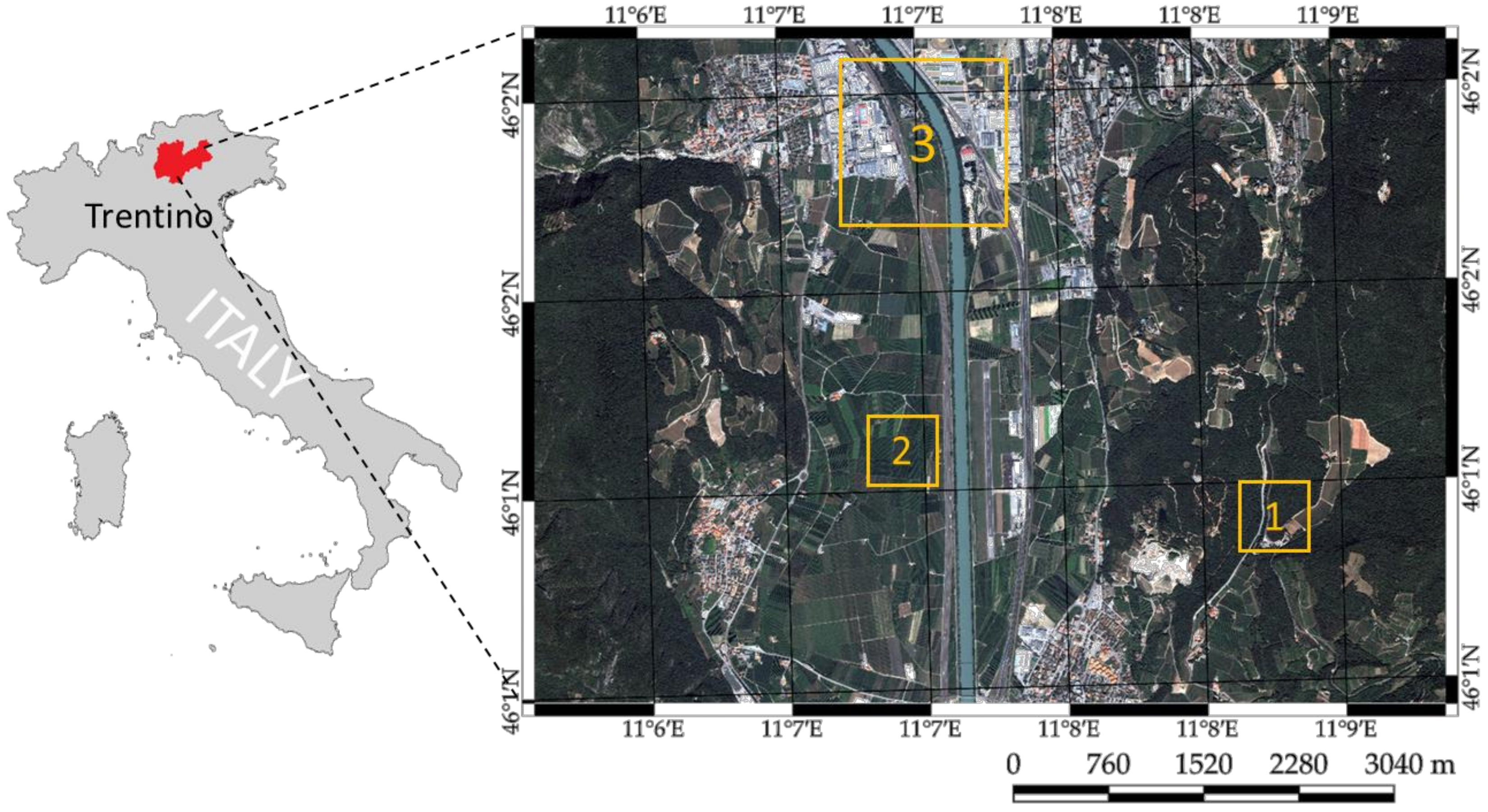
The proposed approach was validated over different areas located in the Trentino region in the north of Italy (Figure 6). These areas show interesting properties from the point of view of orographic conformation and environmental variety. Over a relatively small region it is possible to find: (i) flat regions including precious apple and vineyard fields, and urban, sub-urban and industrial areas with different density and structure; and (ii) hill and mountain environments with a variety of tree species.
Three bi-temporal data sets made up of different couple of images among QuickBird (QB), two WorldView-2 (WV-2) and one GeoEye-1 (GE-1) were constructed over the sample areas (yellow squares in Figure 6). The three datasets were selected such that different types of change are represented. Therefore, dataset 1 shows the transition from forest area to several types of vegetation, dataset 2 shows transitions among different phenological states of crop areas; and dataset 3 shows transitions from vegetation and bare soil (and vice versa) and changes in roofs and roads around an urban area. These datasets allow us to evaluate the complexity of working with multisensor VHR optical images. Details about the three datasets are provided in Table 1. The three satellites show some remarkable differences due to differences in the view angle, the spectral resolution, the number of bands and the spatial resolution.
The QB and GE-1 images have four multispectral bands, whereas WV-2 has eight. The spatial resolution of the QB image is 0.6 m for the panchromatic band and 2.4 m for multispectral bands, whereas WV-2 and GE-1 offer a higher spatial resolution in both panchromatic and multispectral bands with 0.5 m and 2 m, respectively. Table 2 summarizes the characteristics of QB, WV-2 and GE-1 images from the spectral and spatial point of view. The spatial resolution differences imply that the sizes I 1 × J 1 and I 2 × J 2 of X 1 and X 2 images, respectively, are different despite they cover the same surface. The size of QB image in Figure 6 is 8674 × 6300 pixels, whereas the size of WV-2 and GE-1 images is 10297 × 7139 pixels. Thus, pixel-by-pixel comparison cannot be directly applied since the same pixel coordinates in the two images do not correspond to the same position on the ground. Concerning spectral resolution, we can observe that the four primary multi-spectral bands of QB, GE-1 and WV-2 are acquired over similar spectral ranges (e.g., red), but not fully identical (e.g., blue). Similar considerations hold for green and NIR bands.
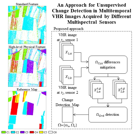
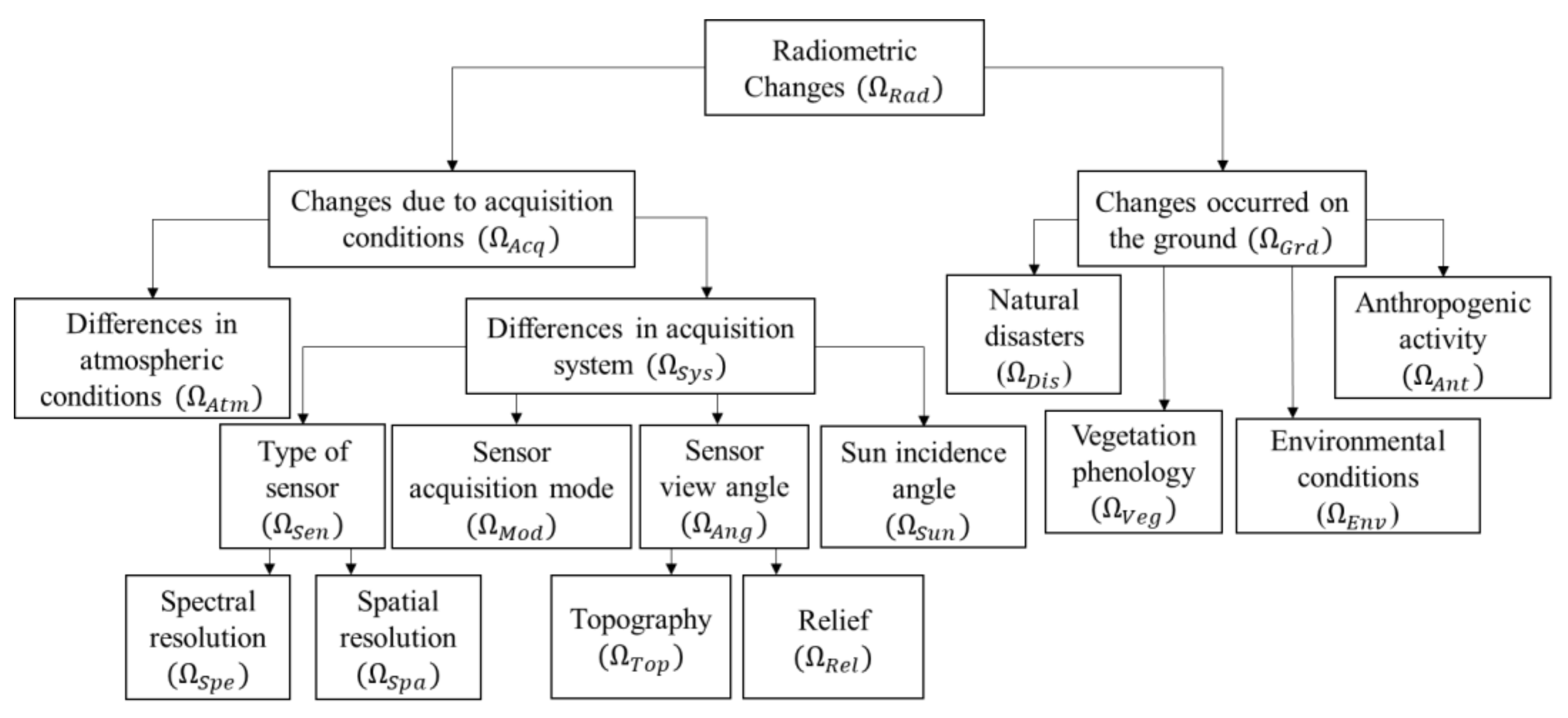
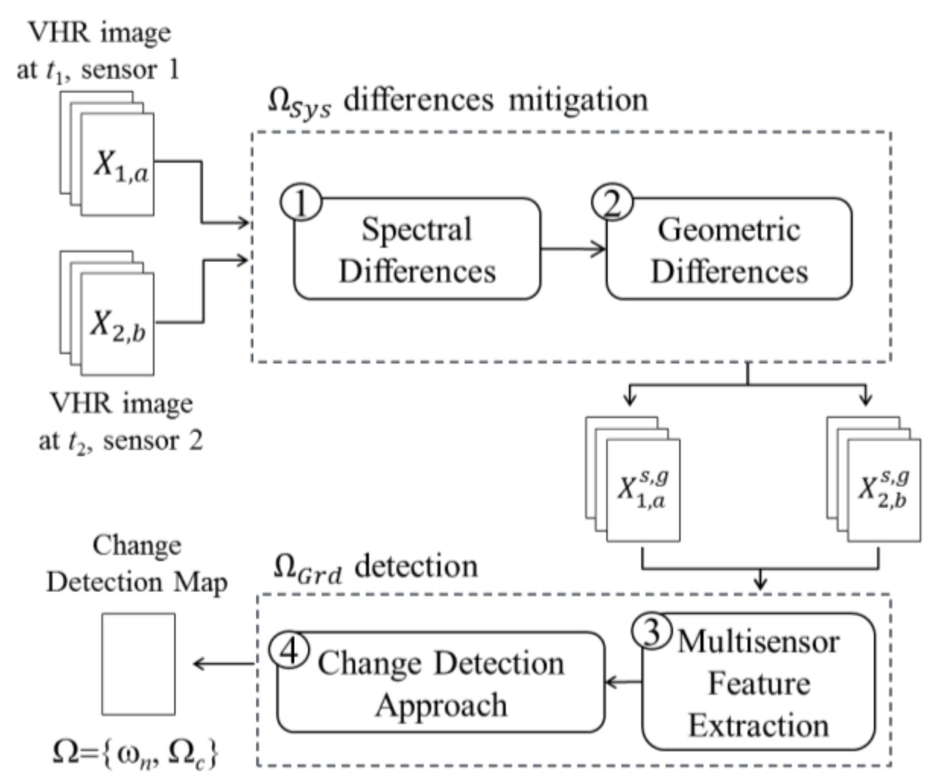
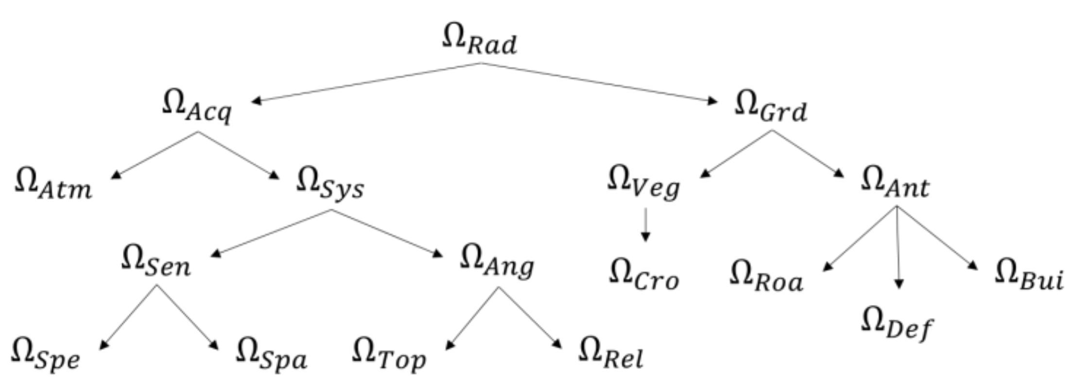
In order to apply the proposed approach, we define the tree of radiometric changes ( Ω Rad ) specific for the considered study areas (one single joint tree is provided for the three datasets), apply mitigation, extract suitable features and perform Ω Grd detection. As a first step, we define the specific tree of radiometric changes ( Ω Rad ) for the considered problem by starting from the general tree given in Figure 1 [5]. The three datasets show changes due to acquisition conditions ( Ω Acq ) and changes occurring on the ground ( Ω Grd ). With regard to Ω Grd , there are changes in the phenological state of the vegetation ( Ω Veg ) (e.g., radiometry of some crops yards, trees, small roads between crop yards ( Ω Cro ), re-vegetation) and changes due to anthropogenic activities ( Ω Ant ) (e.g., changes in road Ω Roa , deforestation Ω Def , roofs Ω Bui and crop planting). It is important to clarify that even though the types of changes can be visually separated by photointerpretation, we do not have enough information to give a precise “from-to” label to them.
Concerning Ω Acq , both atmospheric conditions ( Ω Atm ) and acquisition system ( Ω Sys ) effects are present. Ω Atm is mitigated by means of atmospheric corrections [6]. Ω Sys is related to the type of sensor ( Ω Sen ) and to the sensor view angle ( Ω Ang ). The Ω Ang changes generate small differences in the appearance of objects, leading to geometric distortions, thus to residual misregistration even after proper alignment of images, and to spectral differences when tall buildings are present. We can also see some differences in shadows, which become more critical when high buildings, structures or reliefs are present. Ω Ang and Ω Sen changes are non-relevant from the application viewpoint. Therefore, they are explicitly handled before proceeding to detect Ω Grd and tuning the final CD map. Ω Sys such as the ones due to sensor acquisition mode ( Ω Mod ) are not considered since we are working with passive sensors. Ω Grd like the ones due to natural disasters ( Ω Dis ) or environmental conditions ( Ω Env ) are ignored, since such events did not occur in the considered study area. According to this analysis and to the general taxonomy in Section 2, the tree of radiometric changes for the considered problem becomes the one in Figure 7.
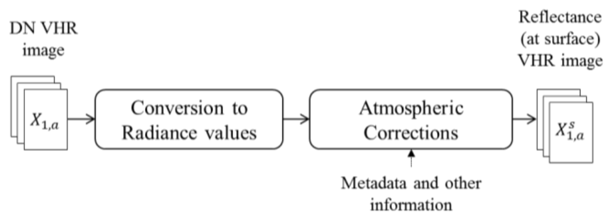
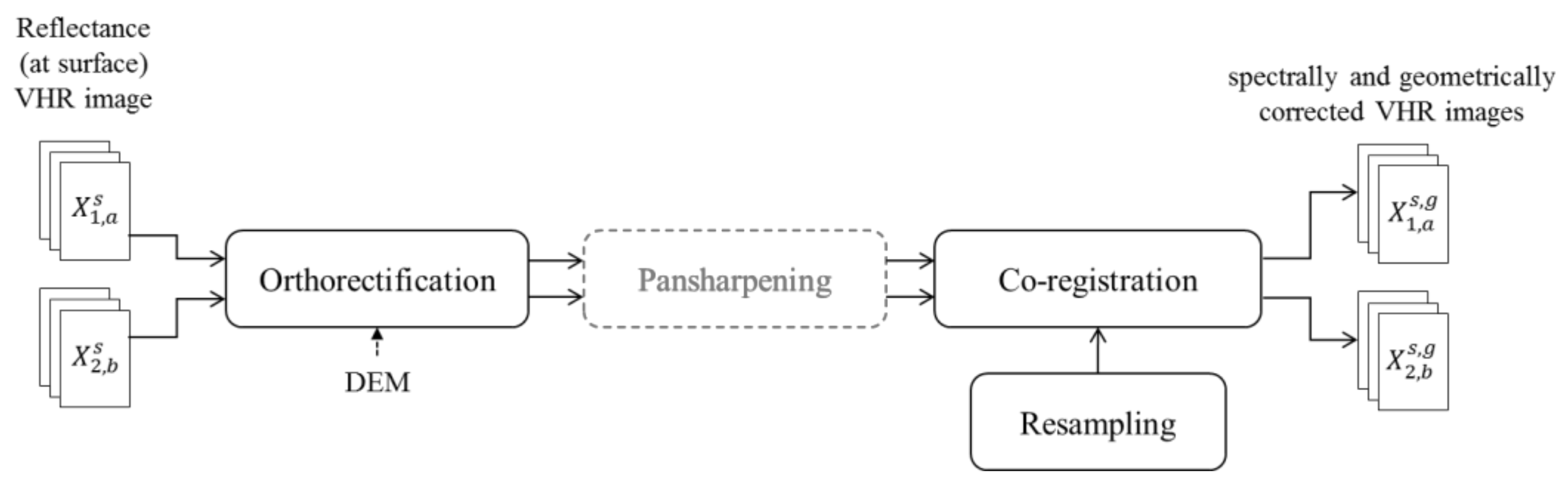
Once the radiometric tree was defined, we performed spectral and geometric differences mitigation. All images were provided by DigitalGlobe Foundation in the context of the “MS-TS—Analysis of Multisensor VHR image Time Series” project [54]. Conversion from DNs to At-Surface Reflectance (ASR) was conducted before delivery by means of the Atmospheric Compensation (AComp) algorithm [6,55,56]. Given the orography of the study area and the possible distortions, we applied orthorectification by using a DEM obtained from LiDAR data [57]. Further distortions appear in dataset 1, since it is located in mountain area, and dataset 3 because of the presence of buildings. Additional pixel-to-pixel problems are also observed due to Ω Ang , and co-registration should be applied.
In order to achieve a better co-registration, PS was applied by means of the Gram–Schmidt method. Here ENVI software package was employed [58]. After PS, the spatial resolution for QB is 0.6 m, and 0.5 m for GE-1 and WV-2 multispectral bands. Co-registration was carried out over the QB–WV-2 and WV-2–GE-1 pairs, covering the whole study area in Figure 6, by using a polynomial function of second order. For the QB 2006 and WV-2 2010 couple, 79 uniformly distributed Ground Control Points (GCP) were selected, whereas 68 uniformly distributed GCP were selected for the WV-2 2011 and GE-1 2011 couple. The WV-2 2010 image was resampled during co-registration. Resampling was performed by means of the nearest neighbor interpolation. 
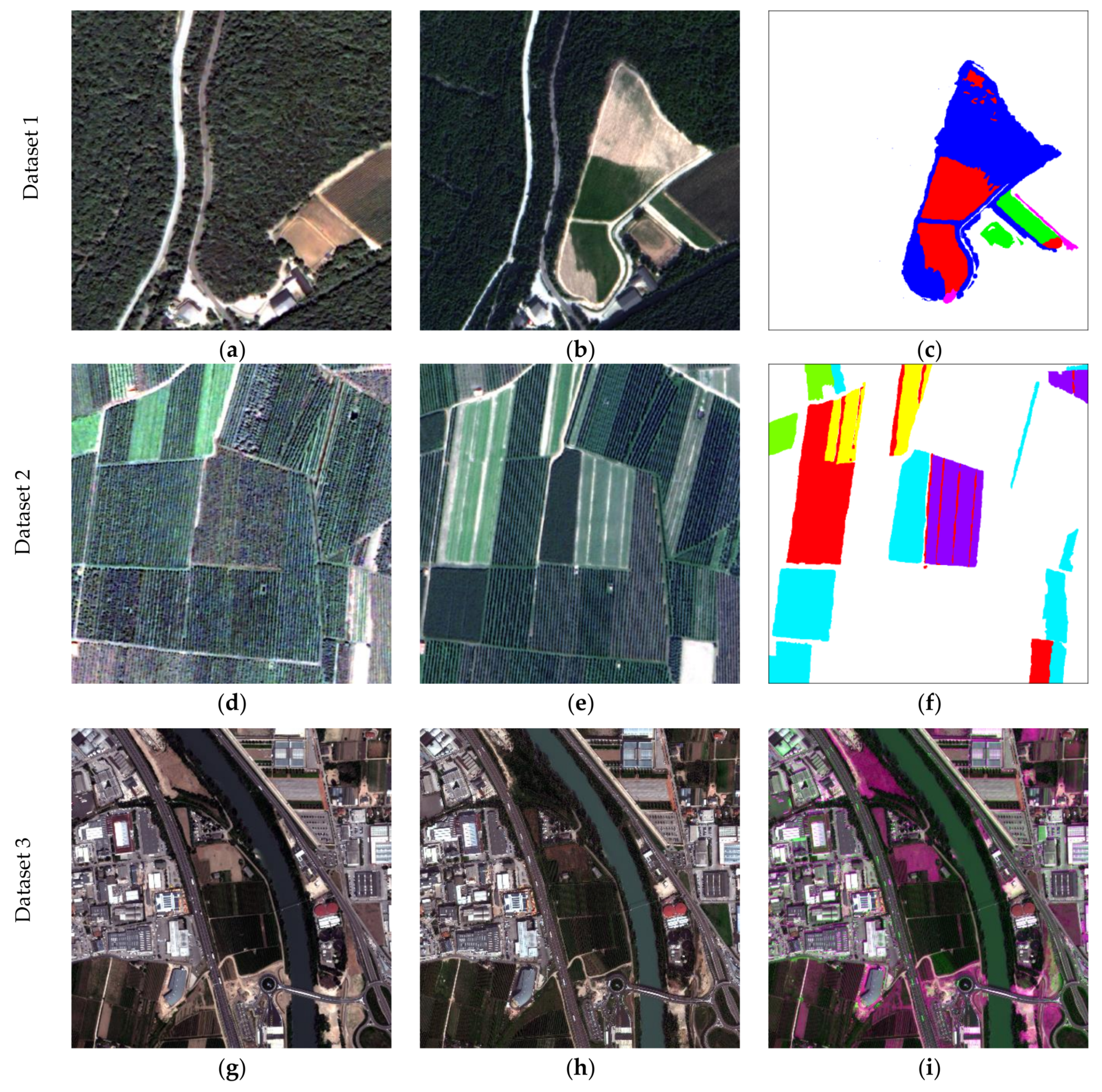
Figure 8 shows the pansharpened multisensor VHR QB, GE-1 and WV-2 images after applying spectral and geometric mitigation in the first and second column, respectively.
Datasets 1 and 2 show a common spatial resolution of 0.6 m and a size of 640 × 640 pixels, whereas dataset 3 shows a common spatial resolution of 0.5 m and a size of 1800 × 1800 pixels. Datasets 1, 2 and 3 appear in first, second and third row of Figure 8, respectively. In order to perform qualitative and quantitative analysis, a reference map for datasets 1 and 2 was defined by photointerpretation and exploiting prior knowledge on the scene as no ground truth was available (see Figure 8c,f, showing 332,414 and 280,928 unchanged pixels (white color) and 77,186 and 128,672 changed pixels (different colors), respectively). For dataset 3, considering the extent of the area and the fact that we have no complete knowledge of the changes occurring on the ground, it was not possible to derive a complete reference map. Thus, quantitative analysis was based on 62808 pixels marked as changed, and 6263 as unchanged, selected by photointerpretation. For comparison purposes, a false color composition of the two acquisitions is provided, green and fuchsia areas represent changes (Figure 8i). Changed pixels in the reference map include Ω Grd , only. For dataset 1, changes from (i) forest to bare soil; (ii) forest to grass; (iii) base soil to grass and (iv) bare soil to some road are identified. For dataset 2, changes from (i) dense vegetation to sparse or light vegetation and vice versa; and (ii) bare soil to vegetation are present. In addition, for dataset 3, changes are from (i) bare soil to vegetation, both dense and sparse; (ii) one to another color of the roofs; and (iii) old to new roads.
Once spectral and geometric mitigation was achieved, mitigation of residual Ω Sys was performed at the level of feature extraction. The selection of the features is therefore designed to detect the residual Ω Sys and the Ω Grd . According to the tree of radiometric changes (Figure 7), residual Ω Sys might be related to Ω Ang , resulting in possible shadows and/or registration noise, whereas Ω Grd includes three type of changes: Ω Cro ,   Ω Roa and Ω Def . Residual Ω Sys due to shadows, due to vegetation or buildings, were detected by means of the method in [59], whereas Ω Sys due to registration noise are negligible. Ω Grd were detected by employing TC and OrE features.
Three main TCs (i.e., Brightness, Greenness and Wetness) and three OrE (Crop mark, Vegetation and Soil) have been studied because of their sensibility to soil content or transitions from-to soil, vegetation, canopy moisture and anthropogenic activities have been studied. Thus, we expect them to properly detect the different changes in the study area, with the exception of some transitions between green areas that do not show up in TC features. These are the cases of datasets 1 and 3, where transitions from forest to grass and crop to grass are misdetected. This is due to the fact that the difference is more in texture rather than in TC features. In order to evaluate and compare the proposed approach, experiments carried on features such as ASR, are also conducted. The detection of changes is obtained by applying CVA to a 3D TC and OrE feature space. However, other features such as IR-MAD [24] could be also used, despite no approaches for automatic detection with these features in multisensor VHR images exist yet. The drawback with IR-MAD is that it requires an end-user interaction to select the most specific components that represent the specific change of interest and to separate among changed and un-changed samples. This is time consuming and makes the approach not fully automatic.
Two experiments were designed: (i) experiment 1 (exp. 1) applies CVA to the transformed ASR bands features; and (ii) experiment 2 (exp. 2) applies CVA to TC (for datasets 1 and 2) or OrE (for dataset 3 which has a large presence or urban areas) features. In exp. 1, the first two selected bands are the Near-IR (NIR) and Red (R) given their high spectral sensibility in the analysis of vegetation and anthropogenic activities. The R bands of QB, GE-1 and WV-2 have quite similar spectral range, whereas the NIR ones do not (see Table 2). Therefore, between NIR1 and NIR2 WV-2 bands, NIR1 (770–995 nm) was selected given that its spectral range better matches to the QB NIR (760–900 nm) and GE-1 NIR (757–853 nm) band spectral range. Another ASR feature to be selected could be the Green or Blue band. Empirical experiments showed a slightly improvement in the final CD accuracy while using Green band instead of Blue one. Therefore, Green band was selected as third feature. In exp. 2, for datasets 1 and 2, TC features were selected based on: (i) the maximum number of TC features that can be derived for each specific sensor, (ii) the radiometric tree of changes; and (iii) the possibility to compare between multisensor TC features. Thus, 4 TC features were derived, bounded by QB properties. In accordance with the radiometric tree, features should be selected that are able to highlight Ω Veg and Ω Ant . Based on the level of comparison between the multisensor TC coefficients, and according to the state-of-the-art, only the first three TC features of each sensor show similar physical meaning. For dataset 3, only three OrE features exist in the literature and are derived by means of the 4 main spectral bands of the sensors.
TC and OrE features were derived directly from the spectrally mitigated data and by using the coefficients in Table 3, Table 4 and Table 5. For TC, only coefficients corresponding to the first three TC feature are present. Here the set of coefficients in [60] was applied to the QB image. The coefficients are derived from the DN feature space (Table 3). There are no TC coefficients derived from TOA values for QB images in the literature. Thus, we applied the QB TC coefficients over the QB DN features, and compared the derived TC features as a higher level primitive. For the WV-2 image, coefficients are applied as given in [61], but to the ASR features instead of TOA ones, as originally derived (Table 4). The OrE features were derived by means of the coefficients shown in Table 5 and as per Equation (1).

3.2. Results and Discussion

In order to assess the effectiveness of the Ω Sys mitigation and the Ω Grd detection approach based on higher-level physical features, CVA was applied by considering the 3D feature space defined above and by means of Equations (2)–(5). We first extracted all the areas that correspond to radiometric changes in the image, by thresholding the magnitude variable. The selection of a threshold T over ρ showed to be a simple and fast way to separate among changed and non-changed pixels. A good separation, among the three dimensions of CVA was guaranteed in average. T was automatically selected by applying a Bayesian decision rule [35] and by following the implementation presented in [62]. In [62], the statistical distribution of the magnitude as a mixture model representing the classes of unchanged and changed pixels is approximated by a Gaussian mixture. Parameters for the statistical distribution are derived by means of the EM algorithm and decision of the threshold is made using a Bayesian minimum cost criterion [46]. The T values for each of the datasets in the two experiments are shown in Table 6.
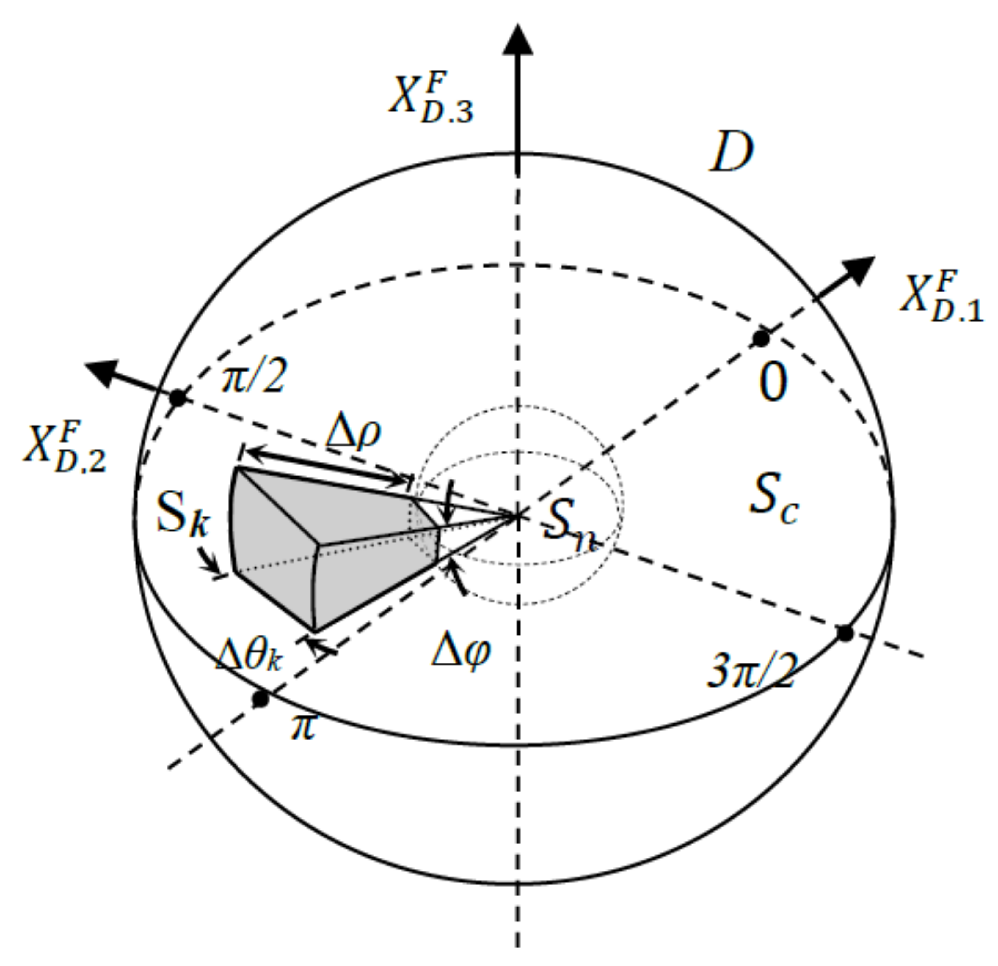
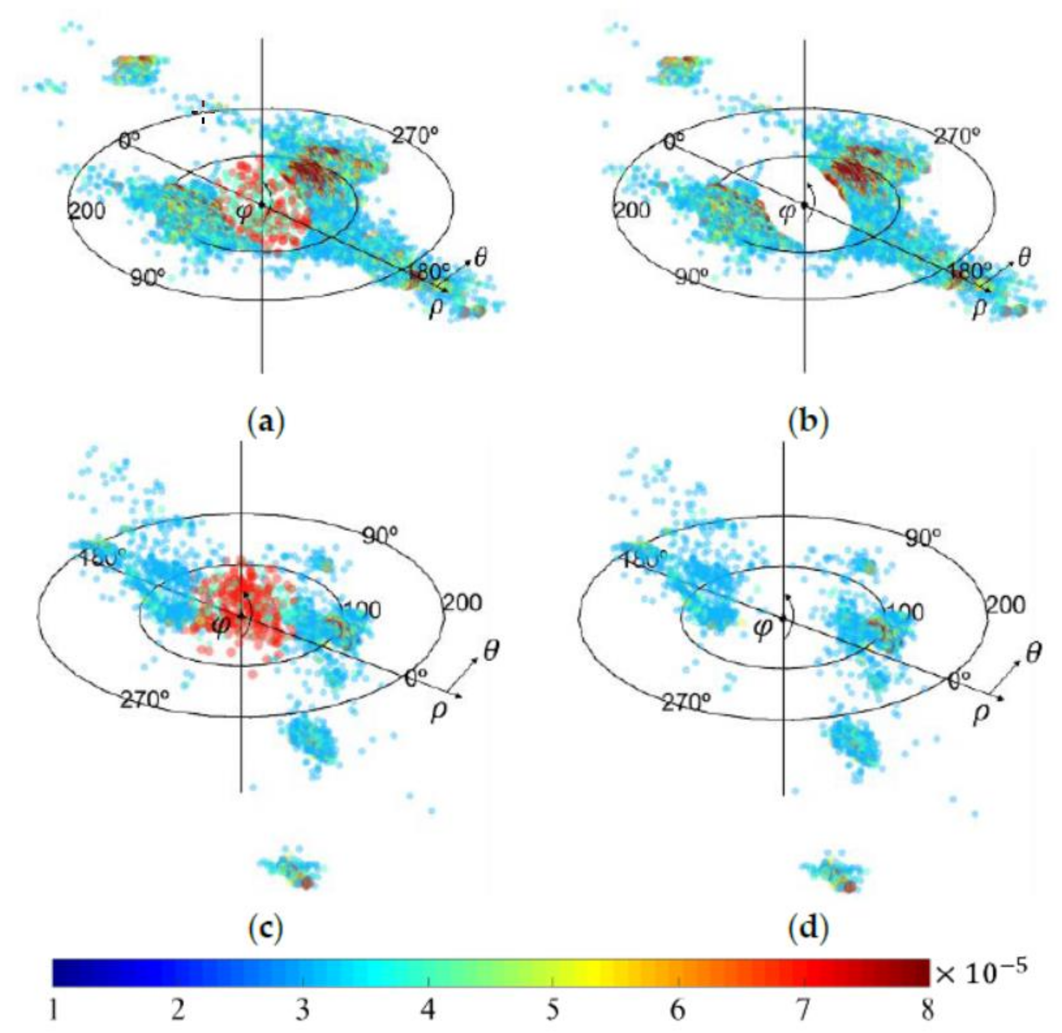
Figure 9 shows the multispectral difference image 3D histogram for the dataset 1, where bigger circles represent higher density (corresponding to the un-changed samples) and small circles represent lower densities (related to the different types of changes). In Figure 9a,c, it is possible to see how X D A S R and X D T C are distributed in a coplanar and sparse way, respectively. This kind of distribution leads to an easier visual interpretation of the X D T C , if compared to X D A S R . In fact, from the 3D histograms in Figure 9, we can see that the coplanar distribution of ASR features does not allow good separation between changes of interest and changes of no interest. A similar behavior is observed between the ASR and OrE features. Right column of Figure 9, presents the changed samples after removing the unchanged ones. Different clusters fit to different S k sectors and are associated with different changes. As we move from X D A S R to X D T C , or X D A S R to X D O r E , it becomes evident how different clusters locate around preferred directions and how the number of clusters increases, making their detection and separation more effective. Separation among different clusters can be performed by automatic or manual methods.
The last step builds the multiple C D m a p by means of the extraction by cancellation strategy. To this end, selection of each of the clusters in the changed region was conducted automatically by means of an adaptation of the TSMO proposed in [36]. The TSMO method yields the same set of thresholds as the conventional Otsu method, but it greatly decreases the required computation time. This is achieved by introducing an intermediate step based on histogram valley estimations, which is used to automatically determine the appropriate number of thresholds for an image. Final multiple CD maps were built by cancelling the remaining Ω Sys and the Ω Grd 
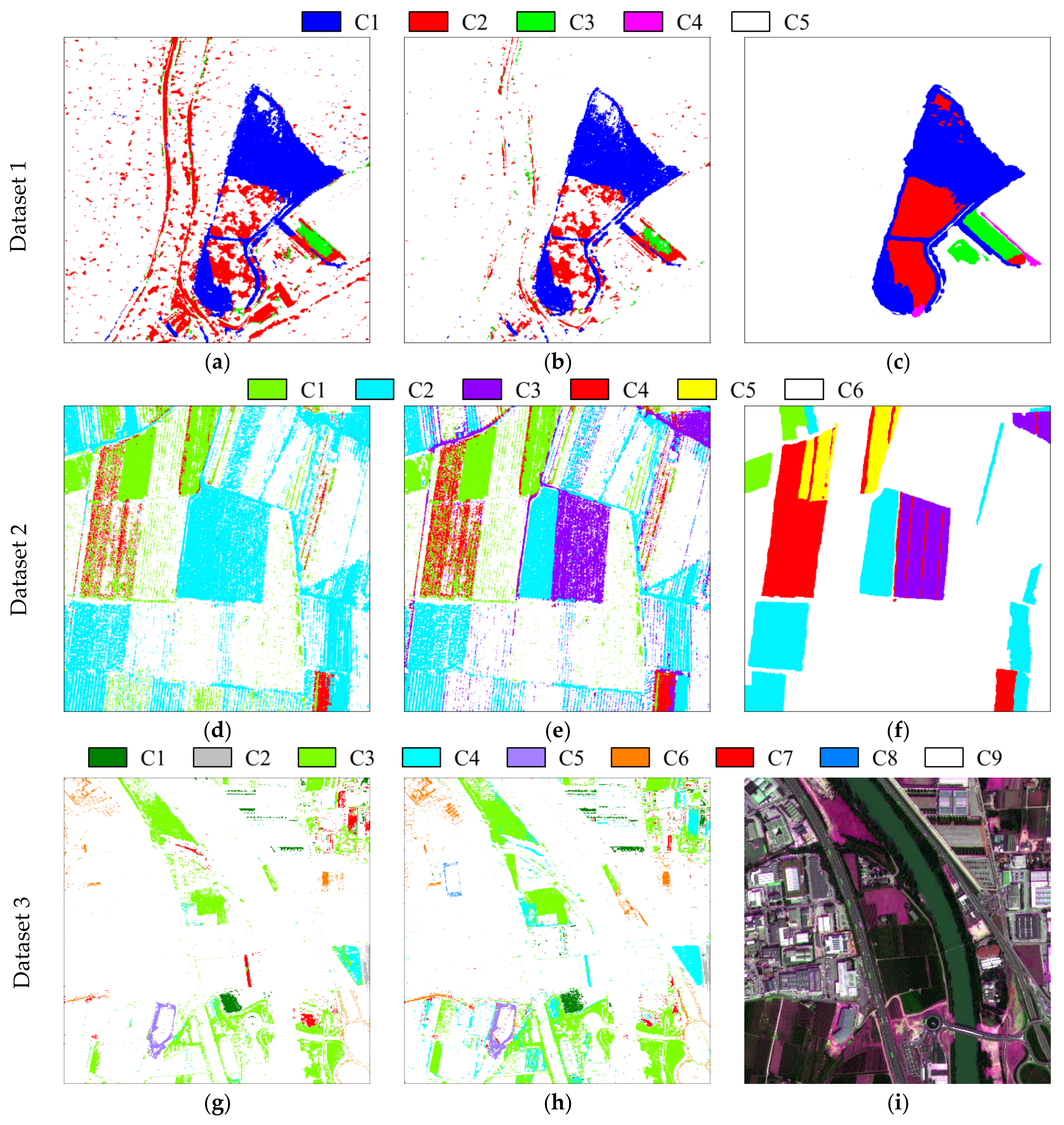
that are out of interest (e.g., cars in road and parking areas, Figure 10). As expected, some vegetation changes that affect more texture rather than TC features are misdetected in datasets 1 and 3. In other words, the selected higher-level physical features are not optimized for those changes, but different higher-level physical features could be selected to properly model most of the types of changes.
In order to perform a qualitative analysis, a comparison of the CD maps with their reference maps (for datasets 1 and 2) and the set of points collected by photointerpretation (dataset 3) was carried out. The comparison pointed out the improvement achieved when working with higher-level physical quantities, specifically for transitions from and to bare soil and different types of crops. This is confirmed when we analyze dataset 1 where changes are mainly from-to vegetation and bare soil. TC features outperform the results obtained when using ASR features (Table 7). As expected, both TC and ASR features have similar problems to identify the change from forest to vegetation. An analogous situation occurs on dataset 2, with changes from-to different types of crops. In this case, TC outperforms ASR being able to separate among changes C2 and C3 (which cannot be discriminated when using ASR features—see Figure 10d–f).
For datasets 1 and 2, the major improvement is related to the decrease of False Alarms (FA) (see Table 7 and Table 8). In dataset 1, the FA correspond to the main road passing through the area and to some of the remaining shadows generated by the tree lines. Even though an index was used to remove the shadows, a small percentage of them remained. In dataset 2, the FA correspond mainly to the linear structures like roads in between the different crops. Moreover, it is possible to observe improvements in terms of detection and separation of the different types of changes. The number of Missed Alarms (MA) decreased as well when working with TC, leading to a better detection of changes, especially when a higher number of changes exist, such as the case of dataset 2. From the quantitative viewpoint, the reduction in both FA and MA reflects in the Overall Accuracy (OA) that increases of about five percent and seven percent for dataset 1 and 2, respectively (see Table 7 and Table 8).
In the case of dataset 3, ASR features poorly separates among C3 and C4 classes that correspond to transitions from bare soil to sparse and dense vegetation, respectively. The number of MA for the class C3 by ASR features is clearly larger than for OrE ones (see Table 9). Moreover, OrE features are able to better detect the classes C2 and C7 than ASR features. C2 and C7 correspond to changes occurring on building roofs and roads renewed in the studied period. Finally, ASR features do not detect class C8 (change in roof color of a building), whereas OrE features do. Other transitions from-to vegetation and bare soil can be seen in the change classes with less MA and FA when the OrE features are used. It is worth noting that changes due to moving cars on roads or in parking areas were considered as non-relevant for this study and thus neglected. From the quantitative perspective, the OA obtained by OrE features increased the overall accuracy of about 2% over that of ASR features. This improvement can be considered relevant given the complexity of the scene with the presence of more types of changes. Proper higher-level physical features, such as some radiometric indexes or texture features, may provide better results. Table 7, Table 8 and Table 9 show the confusion matrices obtained for each dataset in the two experiments.

4. Conclusions and Future Developments

In this paper, an approach for CD in VHR multispectral multisensor optical images has been presented. The proposed approach aims at defining and illustrating a data flow for effectively handling differences due to acquisition sensors. It is based on a general framework for the design of CD systems for VHR multitemporal images presented in [5]. In order to deal with multispectral and multitemporal images acquired by different sensors, it integrates in the general approach the following two concepts: (i) spectral, radiometric and geometric homogenization between images acquired by different sensors; and (ii) detection of multiple changes by means of features that guarantees homogeneity over time and across sensors. Experimental results on real datasets, made-up of VHR bi-temporal and multisensor optical images, confirmed the effectiveness of the proposed block scheme and the improvement achieved by the use of higher-level physical features (i.e., TC and OrE) over the traditional features (i.e., TOA or ASR). In the specific cases of datasets 1 and 2, a major improvement is observed when changes from-to vegetation and bare soil, and different types of crops are considered. This given that the higher-level physical feature (i.e., TC) were selected to highlight such type of changes. In the case of dataset 3, the use of OrE for the detection of changes described above, as well as for changes from-to vegetation and bare soil (i.e., forest to grass, crop to grass, bare soil to grass/forest) and small changes on roads and roofs, resulted in better CD accuracy than that obtained by using ASR. In general, both TC and OrE features allow a better separation and interpretation of Ω Grd by guaranteeing that these changes are distributed in compact and well separated clusters (when in the 3D feature space).
As future developments, further analysis should be carried out to determine which cluster represents a specific type of change, and to define appropriate features for other types of changes. For the mitigation of remaining Ω Sys and the better detection of the Ω Grd , the use of additional features, either in the physical feature space or in the spatial feature space, could help to make the separation and distinction better, thus improving the final OA. Additional improvements from the Ω Sys mitigation process point of view in both spectral and geometric perspective should be considered. For the spectral differences, and given that some of the VHR multisensor optical images have different number of bands and different spectral ranges, the use of regression methods for predicting bands that match from the spectral viewpoint could be considered. For the geometric differences, improvements on the co-registration process by the use of co-registration methods designed for multisensor images could be also explored. Improvements on the detection of building changes could be also integrated.

Acknowledgments

This research is being partially developed under the project “MS-TS—Analysis of Multisensor VHR image Time Series” with DigitalGlobe Foundation. Authors would like to thank DigitalGlobe Foundation for data crosscheck and images provided for the research development.

Author Contributions

All the coauthors made significant contributions to the manuscript. The idea and experiments of the manuscript were conceived by all the coauthors. Yady Tatiana Solano-Correa performed the experiments, analyzed the results and wrote the paper; Francesca Bovolo and Lorenzo Bruzzone provided the background knowledge of change detection in VHR images and helped to revise the manuscript.

Conflicts of Interest

The authors declare no conflicts of interest.

References

  1. Ridd, M.K.; Liu, J. A comparison of four algorithms for change detection in an urban environment. Remote Sens. Environ. 1998, 63, 95–100. [Google Scholar] [CrossRef]
  2. Nemmour, H.; Chibani, Y. Multiple support vector machines for land cover change detection: An application for mapping urban extensions. ISPRS J. Photogramm. Remote Sens. 2006, 61, 125–133. [Google Scholar] [CrossRef]
  3. Desclée, B.; Bogaert, P.; Defourny, P. Forest change detection by statistical object-based method. Remote Sens. Environ. 2006, 102, 1–11. [Google Scholar] [CrossRef]
  4. Yang, X.; Chen, L. Using multi-temporal remote sensor imagery to detect earthquake-triggered landslides. Int. J. Appl. Earth Obs. Geoinf. 2010, 12, 487–495. [Google Scholar] [CrossRef]
  5. Bruzzone, L.; Bovolo, F. A novel framework for the design of change-detection systems for very-high-resolution remote sensing images. Proc. IEEE 2013, 101, 609–630. [Google Scholar] [CrossRef]
  6. Pacifici, F.; Longbotham, N.; Emery, W.J. The importance of physical quantities for the analysis of multitemporal and multiangular optical very high spatial resolution images. IEEE Trans. Geosci. Remote Sens. 2014, 52, 6241–6256. [Google Scholar] [CrossRef]
  7. Schott, J.R.; Salvaggio, C.; Volchok, W.J. Radiometric scene normalization using pseudoinvariant features. Remote Sens. Environ. 1988, 26, 1–16. [Google Scholar] [CrossRef]
  8. Hall, F.G.; Strebel, D.E.; Nickeson, J.E.; Goetz, S.J. Radiometric rectification: Toward a common radiometric response among multidate, multisensor images. Remote Sens. Environ. 1991, 35, 11–27. [Google Scholar] [CrossRef]
  9. Elvidge, C.D.; Yuan, D.; Werackoon, R.D.; Lunetta, R.S. Relative radiometric normalization of Landsat Multispectral Scanner (MSS) data using an automated scattergram controlled regression. Photogramm. Eng. Remote Sens. 1995, 61, 1255–1260. [Google Scholar]
  10. Yang, X.J.; Lo, C.P. Relative radiometric normalization performance for change detection from multi-date satellite images. Photogramm. Eng. Remote Sens. 2000, 66, 967–980. [Google Scholar]
  11. Canty, M.J.; Nielsen, A.A.; Schmidt, M. Automatic radiometric normalization of multitemporal satellite imagery. Remote Sens. Environ. 2004, 91, 441–451. [Google Scholar] [CrossRef] [Green Version]
  12. Canty, M.J.; Nielsen, A.A. Automatic radiometric normalization of multitemporal satellite imagery with the iteratively re-weighted MAD transformation. Remote Sens. Environ. 2008, 112, 1025–1036. [Google Scholar] [CrossRef]
  13. Hong, G.; Zhang, Y. A comparative study on radiometric normalization using high resolution satellite images. Int. J. Remote Sens. 2008, 29, 425–438. [Google Scholar] [CrossRef]
  14. Zhang, H.; Chen, J.; Mao, Z. The research on relative radiometric normalization for change detection of multitemporal images. Image Signal Process. Remote Sens. XV 2009, 7477, 747714. [Google Scholar] [CrossRef]
  15. Klaric, M.N.; Claywell, B.C.; Scott, G.J.; Hudson, N.J.; Sjahputera, O.; Li, Y.; Barratt, S.T.; Keller, J.M.; Davis, C.H. GeoCDX: An automated change detection and exploitation system for high-resolution satellite imagery. IEEE Trans. Geosci. Remote Sens. 2013, 51, 2067–2086. [Google Scholar] [CrossRef]
  16. Dellinger, F.; Delon, J.; Gousseau, Y.; Michel, J.; Tupin, F. Change detection for high resolution satellite images, based on SIFT descriptors and an a contrario approach. In Proceedings of the 2014 IEEE International Geoscience and Remote Sensing Symposium, Quebec City, QC, Canada, 13–18 July 2014; pp. 1281–1284. [Google Scholar]
  17. Camps-Valls, G.; Gomez-Chova, L.; Munoz-Mari, J.; Rojo-Alvarez, J.L.; Martinez-Ramon, M. Kernel-based framework for multitemporal and multisource remote sensing data classification and change detection. IEEE Trans. Geosci. Remote Sens. 2008, 46, 1822–1835. [Google Scholar] [CrossRef] [Green Version]
  18. Lu, D.; Li, G.; Moran, E. Current situation and needs of change detection techniques. Int. J. Image Data Fusion 2014, 5, 13–38. [Google Scholar] [CrossRef]
  19. Lu, D.; Weng, Q. A survey of image classification methods and techniques for improving classification performance. Int. J. Remote Sens. 2007, 28, 823–870. [Google Scholar] [CrossRef]
  20. Hussain, M.; Chen, D.; Cheng, A.; Wei, H.; Stanley, D. Change detection from remotely sensed images: From pixel-based to object-based approaches. ISPRS J. Photogramm. Remote Sens. 2013, 80, 91–106. [Google Scholar] [CrossRef]
  21. Bovolo, F.; Bruzzone, L. The time variable in data fusion: A change detection perspective. IEEE Geosci. Remote Sens. Mag. 2015, 3, 8–26. [Google Scholar] [CrossRef]
  22. Bovolo, F.; Bruzzone, L. A theoretical framework for unsupervised change detection based on change vector analysis in the polar domain. IEEE Trans. Geosci. Remote Sens. 2007, 45, 218–236. [Google Scholar] [CrossRef]
  23. Chen, J.; Gong, P.; He, C.; Pu, R.; Shi, P. Land-use/land-cover change detection using improved change-vector analysis. Photogramm. Eng. Remote Sens. 2003, 69, 369–379. [Google Scholar] [CrossRef]
  24. Nielsen, A.A. The regularized iteratively reweighted MAD method for change detection in multi- and hyperspectral data. IEEE Trans. Image Process. 2007, 16, 463–478. [Google Scholar] [CrossRef] [PubMed]
  25. Lu, D.; Mausel, P.; Brondízio, E.; Moran, E. Change detection techniques. Int. J. Remote Sens. 2004, 25, 2365–2401. [Google Scholar] [CrossRef]
  26. Radke, R.J.; Andra, S.; Al-Kofahi, O.; Roysam, B. Image change detection algorithms: A systematic survey. IEEE Trans. Image Process. 2005, 14, 294–307. [Google Scholar] [CrossRef] [PubMed]
  27. Bayarjargal, Y.; Karnieli, A.; Bayasgalan, M.; Khudulmur, S.; Gandush, C.; Tucker, C.J. A comparative study of NOAA–AVHRR derived drought indices using change vector analysis. Remote Sens. Environ. 2006, 105, 9–22. [Google Scholar] [CrossRef]
  28. Lorena, R.; Dos Santos, J.R.; Shimabukuro, Y.E.; Brown, I.F.; Johann, H. A change vector analysis technique to monitor land use/land cover in sw Brazilian amazon: Acre State. In Proceedings of the Pecora 15/Land Satellite Information IV Conference Integrated Remote Sensing at the Global, Regional and Local Scale, Denver, CO, USA, 10–15 November 2002; pp. 8–15. [Google Scholar]
  29. Kuzera, K.; Rogan, J.; Eastman, J.R. Monitoring vegetation regeneration and deforestation using change vector analysis: Mt. St. Helens study Area. In Proceedings of the ASPRS 2005 Annual Conference, Baltimore, MD, USA, 7–11 March 2005. [Google Scholar]
  30. Kozhikkodan-Veettil, B.; Pereira-Zanardi, R. A comparative study of various urban change detection techniques using high spatial resolution commercial satellite images: Quickbird and Worldview-2. Int. J. Adv. Remote Sens. GIS 2012, 1, 76–84. [Google Scholar]
  31. Tian, J.; Cui, S.; Reinartz, P. Building change detection based on satellite stereo imagery and digital surface models. IEEE Trans. Geosci. Remote Sens. 2014, 52, 406–417. [Google Scholar] [CrossRef] [Green Version]
  32. Karantzalos, K. Recent advances on 2D and 3D change detection in urban environments from remote sensing data. In Computational Approaches for Urban Environments; Geotechnologies and the Environment; Springer: Cham, Switzerland, 2015; pp. 237–272. ISBN 978-3-319-11468-2. [Google Scholar]
  33. Argyridis, A.; Argialas, D.P. Building change detection through multi-scale GEOBIA approach by integrating deep belief networks with fuzzy ontologies. Int. J. Image Data Fusion 2016, 7, 148–171. [Google Scholar] [CrossRef]
  34. Zanotta, D.C.; Bruzzone, L.; Bovolo, F.; Shimabukuro, Y.E. An adaptive semisupervised approach to the detection of user-defined recurrent changes in image time series. IEEE Trans. Geosci. Remote Sens. 2015, 53, 3707–3719. [Google Scholar] [CrossRef]
  35. Carson, C.; Belongie, S.; Greenspan, H.; Malik, J. Blobworld: Image segmentation using expectation-maximization and its application to image querying. IEEE Trans. Pattern Anal. Mach. Intell. 2002, 24, 1026–1038. [Google Scholar] [CrossRef]
  36. Huang, D.Y.; Lin, T.W.; Hu, W.C. Automatic multilevel thresholding based on two-stage Otsu’s method with cluster determination by valley estimation. Int. J. Innov. Comput. Inf. Control 2011, 7, 5631–5644. [Google Scholar]
  37. Marchesi, S.; Bovolo, F.; Bruzzone, L. A context-sensitive technique robust to registration noise for change detection in VHR multispectral images. IEEE Trans. Image Process. 2010, 19, 1877–1889. [Google Scholar] [CrossRef] [PubMed]
  38. Lu, P.; Stumpf, A.; Kerle, N.; Casagli, N. Object-oriented change detection for landslide rapid mapping. IEEE Geosci. Remote Sens. Lett. 2011, 8, 701–705. [Google Scholar] [CrossRef]
  39. Molinier, M.; Laaksonen, J.; Hame, T. Detecting man-made structures and changes in satellite imagery with a content-based information retrieval system built on self-organizing maps. IEEE Trans. Geosci. Remote Sens. 2007, 45, 861–874. [Google Scholar] [CrossRef]
  40. Longbotham, N.; Chaapel, C.; Bleiler, L.; Padwick, C.; Emery, W.J.; Pacifici, F. Very high resolution multiangle urban classification analysis. IEEE Trans. Geosci. Remote Sens. 2012, 50, 1155–1170. [Google Scholar] [CrossRef]
  41. Matasci, G.; Longbotham, N.; Pacifici, F.; Kanevski, M.; Tuia, D. Understanding angular effects in VHR imagery and their significance for urban land-cover model portability: A study of two multi-angle in-track image sequences. ISPRS J. Photogramm. Remote Sens. 2015, 107, 99–111. [Google Scholar] [CrossRef]
  42. Duca, R.; Frate, F.D. Hyperspectral and multiangle CHRIS-PROBA images for the generation of land cover maps. IEEE Trans. Geosci. Remote Sens. 2008, 46, 2857–2866. [Google Scholar] [CrossRef]
  43. Barnsley, M.J.; Settle, J.J.; Cutter, M.A.; Lobb, D.R.; Teston, F. The PROBA/CHRIS mission: A low-cost smallsat for hyperspectral multiangle observations of the Earth surface and atmosphere. IEEE Trans. Geosci. Remote Sens. 2004, 42, 1512–1520. [Google Scholar] [CrossRef]
  44. Han, Y.; Bovolo, F.; Bruzzone, L. An approach to fine coregistration between very high resolution multispectral images based on registration noise distribution. IEEE Trans. Geosci. Remote Sens. 2015, 53, 6650–6662. [Google Scholar] [CrossRef]
  45. Zhang, Y.; Hong, G. An IHS and wavelet integrated approach to improve pan-sharpening visual quality of natural colour IKONOS and QuickBird images. Inf. Fusion 2005, 6, 225–234. [Google Scholar] [CrossRef]
  46. Bruzzone, L.; Fernández-Prieto, D. Automatic analysis of the difference image for unsupervised change detection. IEEE Trans. Geosci. Remote Sens. 2000, 38, 1171–1182. [Google Scholar] [CrossRef]
  47. Malila, W.A. Change Vector Analysis: An Approach for Detecting Forest Changes with Landsat; Purdue University, Purdue e-Pubs: West Lafayette, IN, USA, 1980; pp. 326–335. [Google Scholar]
  48. Bovolo, F. A multilevel parcel-based approach to change detection in very high resolution multitemporal images. IEEE Geosci. Remote Sens. Lett. 2009, 6, 33–37. [Google Scholar] [CrossRef]
  49. Kauth, R.J.; Thomas, G.S. The tasselled cap—A graphic description of the spectral-temporal development of agricultural crops as seen by Landsat. In Proceedings of the Symposium on Machine Processing of Remotely Sensed Data, West Lafayette, Indiana, 29 June–1 July 1976; pp. 4B-41–4B-50. [Google Scholar]
  50. Agapiou, A.; Alexakis, D.D.; Sarris, A.; Hadjimitsis, D.G. Orthogonal equations of multi-spectral satellite imagery for the identification of un-excavated archaeological sites. Remote Sens. 2013, 5, 6560–6586. [Google Scholar] [CrossRef]
  51. Bruzzone, L.; Fernández-Prieto, D. A minimum-cost thresholding technique for unsupervised change detection. Int. J. Remote Sens. 2000, 21, 3539–3544. [Google Scholar] [CrossRef]
  52. Bovolo, F.; Bruzzone, L. An adaptive thresholding approach to multiple-change detection in multispectral images. In Proceedings of the 2011 IEEE International Geoscience and Remote Sensing Symposium, Vancouver, BC, Canada, 24–29 July 2011; pp. 233–236. [Google Scholar]
  53. Persello, C. Advanced Techniques for the Classification of Very High Resolution and Hyperspectral Remote Sensing Images. Ph.D. Thesis, University of Trento, Trento, Italy, 2010. [Google Scholar]
  54. DigitalGlobe Foundation. Available online: http://foundation.digitalglobe.com/ (accessed on 15 January 2018).
  55. Pacifici, F. Atmospheric Compensation in Satellite Imagery. US Patent 9396528B2, 19 July 2016. [Google Scholar]
  56. DigitalGlobe Atmospheric Compensation. Available online: http://explore.digitalglobe.com/AComp.html?utm_source=blog&utm_medium=website&utm_campaign=AComp (accessed on 15 January 2018).
  57. Paris, C.; Bruzzone, L. A three-dimensional model-based approach to the estimation of the tree top height by fusing low-density LiDAR data and very high resolution optical images. IEEE Trans. Geosci. Remote Sens. 2015, 53, 467–480. [Google Scholar] [CrossRef]
  58. ENVI—The Leading Geospatial Analytics Software|Harris Geospatial. Available online: http://www.harrisgeospatial.com/SoftwareTechnology/ENVI.aspx (accessed on 15 January 2018).
  59. Tsai, V.J.D. A comparative study on shadow compensation of color aerial images in invariant color models. IEEE Trans. Geosci. Remote Sens. 2006, 44, 1661–1671. [Google Scholar] [CrossRef]
  60. Yarbrough, L.D.; Easson, G.; Kuszmaul, J.S. QuickBird 2 Tasseled Cap transform coefficients: A comparison of derivation methods. In Proceedings of the Pecora 16 “Global Priorities in Land Remote Sensing”, Sioux Falls, SD, USA, 23–27 October 2005. [Google Scholar]
  61. Yarbrough, L.D.; Navulur, K.; Ravi, R. Presentation of the Kauth–Thomas transform for WorldView-2 reflectance data. Remote Sens. Lett. 2014, 5, 131–138. [Google Scholar] [CrossRef]
  62. EM Image Segmentation—File Exchange—MATLAB Central. Available online: http://it.mathworks.com/matlabcentral/fileexchange/10956-em-image-segmentation (accessed on 8 March 2018).
Figure 1. General tree of radiometric changes for the multisensor Very High Resolution (VHR) images case [5].
Remotesensing 10 00533 g001
Figure 2. Block scheme of the proposed approach to Change Detection (CD) in multitemporal multisensor VHR optical images.
Remotesensing 10 00533 g002
Figure 3. Block scheme for mitigation of Ω Spe in multisensor VHR images.
Remotesensing 10 00533 g003
Figure 4. Block scheme followed for the mitigation of geometric differences in multisensor VHR images.
Remotesensing 10 00533 g004
Figure 5. Regions of interest for Change Vector Analysis (CVA) in spherical coordinates: domain D of Spectral Change Vectors (SCVs) in X D F , sphere S n of no-changes, spherical shell S c including changes and solid truncated cone S k associated to a generic change k [34].
Remotesensing 10 00533 g005
Figure 6. Area of interest, Trentino region in the North of Italy.
Remotesensing 10 00533 g006
Figure 7. Tree of radiometric changes for the considered problem.
Remotesensing 10 00533 g007
Figure 8. True color composition of the pansharpened multispectral multisensor VHR datasets: (a,d) QB image acquired in July 2006; (b,e) WV-2 image acquired in August 2010; (g) WV-2 image acquired in May 2011; and (h) GE-1 image acquired in September 2011; (c,f) Reference maps; and (i) false color composition for dataset 3 (magenta and green shades highlight changes).
Remotesensing 10 00533 g008
Figure 9. Histogram in spherical coordinates of (a) X D A S R , (c) X D T C , and changed samples after thresholding ρ for (b) At-Surface Reflectance (ASR) and (d) TC features.
Remotesensing 10 00533 g009
Figure 10. Change detection maps obtained by CVA in 3D applied to the three datasets in: (a,d,g) ASR features; (b,e) TC features; and (h) Orthogonal features. (c,f) Reference map; and (i) false color composition for dataset 3 (magenta and green shades highlight changes).
Remotesensing 10 00533 g010
Table 1. Datasets description. QB: QuickBird; WV: WorldView; GE: GeoEye.
Dataset 1 and 2Dataset 3
t 1 t 2 t 1 t 2
SensorQBWV-2WV-2GE-1
Acquisition dateJuly 2006August 2010May 2011September 2011
Off-nadir angle14.1° 19.3° 7.8° 14.4°
Table 2. Main characteristics of QuickBird, WorldView-2 and GeoEye-1 optical sensors [53].
SatelliteQuickBirdWorldView-2GeoEye-1
Bands (nm)445–900 (pan)450–800 (pan)450–800 (pan)
400–450 (coastal)
450–520 (blue)450–510 (blue)450–510 (blue)
520–600 (green)510–580 (green)510–580 (green)
585–626 (yellow)
630–690 (red)630–690 (red)655–690 (red)
705–745 (red edge)
760–900 (NIR)770–895 (NIR 1)780–920 (NIR)
860–1040 (NIR 2)
Spatial Resolution (m)0.610.460.41
2.441.841.65
Table 3. Tasseled Cap (TC) coefficients for QuickBird Digital Numbers (DN) values [60].
BandsBrightness (TC1)Greenness (TC2)Wetness (TC3)
B10.319−0.1210.652
B20.542−0.3310.375
B30.490−0.517−0.639
B40.6040.780−0.163
Table 4. TC coefficients for WorldView-2 TOA values [61].
BandsBrightness (TC1)Greenness (TC2)Wetness and shadows (TC3)
B1−0.060−0.140−0.271
B20.012−0.206−0.316
B30.126−0.216−0.317
B40.313−0.314−0.243
B50.412−0.411−0.256
B60.4830.096−0.097
B7−0.1610.601−0.743
B80.6730.5040.202
Table 5. Orthogonal coefficients for WorldView-2 and GeoEye-1 [50].
Orthogonal ComponentBlueGreenRedNIR
WV-2Crop Mark−0.38−0.710.20−0.56
Vegetation−0.37−0.39−0.670.52
Soil0.090.27−0.71−0.65
GE-1Crop Mark−0.39−0.730.17−0.54
Vegetation−0.35−0.37−0.680.54
Soil0.080.27−0.71−0.65
Table 6. Magnitude ( T ) threshold values for the three datasets in Exp. 1 and 2.
DatasetExp. T
110.060
20.080
210.025
20.030
310.090
20.060
Table 7. Confusion matrices for dataset 1 in Exp. 1 and Exp. 2.
Exp.Changes FoundActual Changes
C1C2C3C4C5Reliability
1C139775596910212993.38%
C2220695001501442842822.79%
C3952427128207752.24%
C4000000.00%
C53765130902718132729978093.48%
Accuracy86.93%40.96%36.02%0.00%90.18%
Overall Accuracy85.81%
2C13655825092091096.69%
C224128153135594657143.87%
C302146442115255.03%
C4000000.00%
C56785147863829136332378192.36%
Accuracy79.9%35.15%21.72%0.00%97.40%
Overall Accuracy90.32%
Table 8. Confusion matrices for dataset 2 in Exp. 1 and Exp. 2.
Exp.Changes FoundActual Changes
C1C2C3C4C5C6Reliability
1C153816110387122861640812.10%
C21424024219330356044740636.35%
C30000000.00%
C418050947210268877.40%
C50000000.00%
C611987973364313800116921442688.53%
Accuracy79.85%83.45%0.00%25.48%0.00%76.33%
Overall Accuracy65.80%
2C13269831044712423121978.52%
C266379712910222930156.13%
C311677319534371321508049.81%
C45931961547651415677.61%
C50000000.00%
C6322994663000758397122019490.08%
Accuracy48.51%78.74%84.84%41.58%0.00%78.38%
Overall Accuracy72.37%
Table 9. Confusion matrices for dataset 3 in Exp. 1 and Exp. 2.
Exp.Changes FoundActual Changes
C1C2C3C4C5C6C7C8C9Reliability
1C190500000000100%
C202060000000100%
C300164233400001182.64%
C4002745000160091.28%
C500002400000100%
C600000400001297.09%
C730068001950073.31%
C80000000000.0%
C972502033920198892136278597.18%
Accuracy55.42%100%87.71%36.17%100%66.89%65.00%0.00%99.96%
Overall Accuracy96.75%
2C1129400000009193.43%
C202060000000100%
C300179213400002291.99%
C40027105200160096.07%
C500002400000100%
C6000005820014380.27%
C7000000158020543.53%
C80000000660100%
C9339026580161101476234798.90%
Accuracy79.24%100%97.13%84.57%100%97.32%55.63%30.98%99.27%
Overall Accuracy98.07%

