3-D Characterization of Vineyards Using a Novel UAV Imagery-Based OBIA Procedure for Precision Viticulture Applications

Abstract

Precision viticulture has arisen in recent years as a new approach in grape production. It is based on assessing field spatial variability and implementing site-specific management strategies, which can require georeferenced information of the three dimensional (3D) grapevine canopy structure as one of the input data. The 3D structure of vineyard fields can be generated applying photogrammetric techniques to aerial images collected with Unmanned Aerial Vehicles (UAVs), although processing the large amount of crop data embedded in 3D models is currently a bottleneck of this technology. To solve this limitation, a novel and robust object-based image analysis (OBIA) procedure based on Digital Surface Model (DSM) was developed for 3D grapevine characterization. The significance of this work relies on the developed OBIA algorithm which is fully automatic and self-adaptive to different crop-field conditions, classifying grapevines, and row gap (missing vine plants), and computing vine dimensions without any user intervention. The results obtained in three testing fields on two different dates showed high accuracy in the classification of grapevine area and row gaps, as well as minor errors in the estimates of grapevine height. In addition, this algorithm computed the position, projected area, and volume of every grapevine in the field, which increases the potential of this UAV- and OBIA-based technology as a tool for site-specific crop management applications.

1. Introduction

Vineyard yield and grape quality are variable and depend on several field and crop-related factors, so that studying the influence and spatial distribution of these factors allows grape growers to improve vineyard management according to quality and productivity parameters [1]. In this context, precision viticulture (PV) has arisen in recent years as a new approach in grape production, which is based on assessing intra- and inter- crop-field spatial variability and implementing site-specific crop management systems [2]. Its ultimate objective is to optimize crop production and profitability through a reduction in production inputs (e.g., pesticides, fertilizers, machinery, fuel, water, etc.) and, consequently, diminish potential damage to the environment due to the over-application of inputs [3,4]. To design site-specific management strategies, georeferenced information of the grapevine canopy structure and its variability at the field scale are required as input data, since plant architecture is one of the most important traits for the characterization and monitoring of fruit trees [5]. As an alternative to time-consuming on-ground methods traditionally used to collect crop data, remote sensing offers the possibility of a rapid assessment of large vineyard areas [6,7]. Within the PV context, aerial remote sensing in the optical domain offers a potential way to map crop structure, such as vegetation cover fraction, row orientation, or leaf area index. This information can be registered in a non-destructive way and can be later used in decision support tools [8]. Among the remote sensing platforms, Unmanned Aerial Vehicles (UAVs) stand out because of their unprecedented high spatial resolution and flexibility of flight scheduling, which are essential for the accurate and timely monitoring of the crop. To date, UAVs have been used for a wide range of purposes in PV, such as the assessment of water status [9], disease detection [10], vine canopy characterization [5,8,11,12], and the study of spatial variability in yield and berry composition [13]. The development of new techniques based on UAV imagery is therefore a required target for PV, since UAVs are rapidly replacing other platforms for vineyard monitoring [12].

In addition to the aforementioned advantages, UAVs are able to fly at low altitudes with high image overlap, which permits the generation of Digital Surface Models (DSMs) using photo-reconstruction techniques or artificial vision [14,15,16,17]. The UAV-based DSMs have recently been used in agricultural applications, for example to discriminate weeds in herbaceous crops at early stage [18,19]; to calculate tree area, height, and crown volume in olive orchards and to quantify the impact of different pruning treatments [20,21]; to isolate vine pixel as intermediate stage and to assess biomass volume [22]. Processing the large amount of detailed crop data embedded in UAV images and DSMs requires the implementation of robust and automatic image analysis procedures. In the last few years, object-based image analysis (OBIA) techniques have reached high levels of automation and adaptability to ultra-high spatial resolution images and provide better solutions to the problem of pixel heterogeneity in comparison with conventional pixel-based methods [23]. The elemental analysis unit of OBIA is the “object”, which groups adjacent pixels with homogenous spectral values. Then, OBIA combines the spectral, topological, and contextual information of these objects to address complicated classification issues. Successful examples of OBIA applications include agricultural [24,25,26,27,28], grassland [29,30], and forest scenarios [31,32,33]. Therefore, the combination of UAV-based DSM and OBIA enables to tackle the significant challenge of automating image analysis [19], which represents a relevant advance in agronomy science.

In this investigation, a novel OBIA procedure was developed to characterize the 3D structure of the grapevines without any user intervention. The 3D information was generated by combining aerial images collected with a low-cost camera attached to an UAV and photo-reconstructed digital surface models (DSMs). Specific objectives included: (1) automatic classification of grapevines and row gaps (missing vine plants) without user intervention, overcoming the problem of spectral similarity with inter-row vegetation (cover-crop or weeds) and (2) automatic estimation of individual grapevines position (geographic coordinates) and dimensions (projected area, height, and volume). In addition, the potential applications of the outputs obtained with this methodology were discussed, including agronomical studies as well as for designing site-specific management strategies in the context of precision viticulture.

2. Materials and Methods

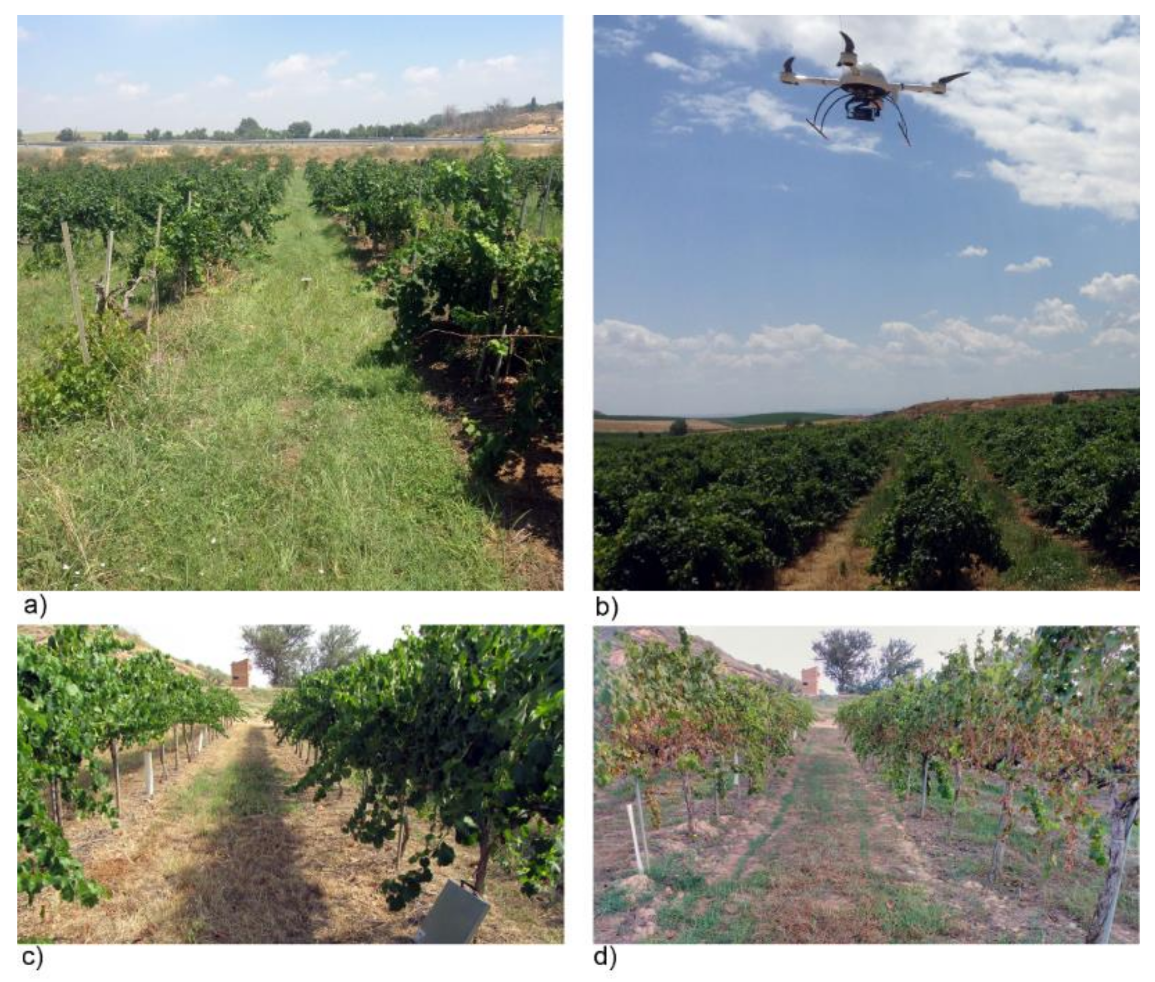
2.1. Study Fields and UAV Flights

The experiment was carried out in three different commercial vineyards located in the province of Lleida, Northeastern Spain (

Table 1. Main characteristics of the studied fields. Coordinates are in the WGS84, UTM zone 31N reference system.

Field	Grape Variety	Studied Area (m2)	Central Coordinates (X, Y)
A	Merlot	4925	291,009 E; 4,613,392 N
B	Albariño	4415	291,303 E; 4,614,055 N
C	Chardonnay	2035	290,910 E; 4,616,282 N

). The private company Raimat owner of the fields authorized this investigation and the UAV flights with an agreement in written. Vines were drip-irrigated and trellis-trained in all the vineyards, with the rows separated by 3 m and vine spacing of 2 m, and inter-row cover crops (Figure 1a), which has been reported in previous studies as a complex scenario due to the spectral similarity between vines and green cover crops [9,12]. Vines management was mainly focused on wine production. The rows were north-south generally oriented for field A and B, and northwest-southeast for field C.

The remote images were acquired with a low-cost RGB (R: red; G: green; B: blue) commercial off-the-shelf camera, model Olympus PEN E-PM1 (Olympus Corporation, Tokyo, Japan) mounted in a quadcopter model MD4-1000 (microdrones GmbH, Siegen, Germany) (Figure 1b). Technical specifications of the sensor are given in

Table 2. Technical specifications of the imaging sensor on board the Unmanned Aerial Vehicle (UAV).

Sensor Size (mm)	Pixel Size (mm)	Sensor Resolution (pixels)	Focal Length (mm)	Radiometric Resolution (bit)	Image Format
17.3 × 13.0	0.0043	4032 × 3024	14	8	JPEG

. The UAV can fly either manually by radio control (1000 m control range) or autonomously, with the aid of its Global Navigation Satellite System (GNSS) receiver and its waypoint navigation system. The UAV is battery powered and can load any sensor weighing up to 1.25 kg.

Two flights were performed in each field, the first one on 29 July 2015 and the second one on 16 September 2015, depicting two different crop stages. In late July, the grapevine canopy was fully developed, with most of berries beginning to touch or touching, corresponding to 77 and 79 growth stage of the BBCH (Biologische Bundesantalt, Bundessortenamt, and Chemische Industrie) scale [34] (Figure 1c); while in September, the grapes had been machine-harvested (being at 91 growth stage of the BBCH scale), and consequently, the grapevine canopy was less dense (Figure 1d).

This approach, consisting of three fields at two crop stages, made it possible to analyze a wide range of situations to ensure the robustness of the OBIA procedure. The flights were performed at 30 m flight altitude, with a resulting spatial resolution of 1 cm pixel size and a ground image dimension of 37 × 28 m. The UAV route was programmed to take images continuously at 1-second intervals, thus resulting in a 93% of forward lap, and to produce a side lap of 60%. These overlaps were high enough to achieve the 3D reconstruction of woody crops according to previous investigations [20]. The flight operations fulfilled the list of requirements established by the Spanish National Agency of Aerial Security, including the pilot license, safety regulations, and limited flight distance [35].

2.2. DSM and Orthomosaic Generation

The DSM with height information and orthomosaic were generated using the Agisoft PhotoScan Professional Edition software (Agisoft LLC, St. Petersburg, Russia) version 1.2.4 build 1874. The mosaicking process was fully automatic, with the exception of the manual localization of 5 ground control points in the corners and in the center of each field with a Trimble GeoXH 2008 Series (Trimble, Sunnyvale, CA, USA) to georeference the DSM and orthomosaic. The whole automatic process involved three principal stages: (1) aligning images; (2) building field geometry; and (3) ortho-photo generation. First, the camera position for each image and common points in the images were located and matched, which facilitated the refinement of camera calibration parameters. Next, the software searched for more common points in the images to create a dense 3D point cloud (Figure 2) that was used as basis to generate the DSM, which was saved in greyscale tiff format. Finally, the individual images were projected over the DSM, and the orthomosaic was generated (Figure 3). The methodology to build these accurate geomatic products has been validated in previous research [20,36]. The orthomosaics were only employed for validation purposes. More details about the Photoscan functioning are given in [37], and information about the processing parameters of the software are shown in

Table 3. Processing parameters selected for Digital Surface Model (DSM) and orthomosaic generation procedure by Agisoft Photoscan software.

Preference Setting	Control Parameter	Selected Setting
Alignment parameters	Accuracy	High
	pair preselection	Disabled
Dense point cloud	Quality	High
	depth filtering	Mild
DSM	Coordinate system	WGS84/UTM zone 31 N
	source data	Dense cloud
Orthomosaic	Blending mode	Mosaic

. Radiometric corrections were not applied to the images as the proposed algorithm uses only DSM values, with independence of the spectral information of the images, which reduces time and optimizes the procedure.

2.3. OBIA Algorithm

The OBIA algorithm for the detection and characterization of grapevines was developed using Cognition Network programming language with the eCognition Developer 9 software (Trimble GeoSpatial, Munich, Germany). The algorithm is fully automatic, it therefore requires no user intervention, and also has the benefit of self-adapting to the different crop-field conditions, such as row-orientation, row and vine spacing, field slope, inter-row cover crops or grapevine dimensions.

The algorithm consisted of a sequence of phases (Figure 3), using only the DSM image as input, which are described as follows:

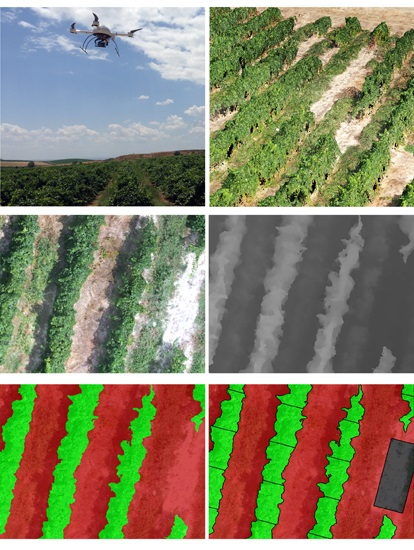
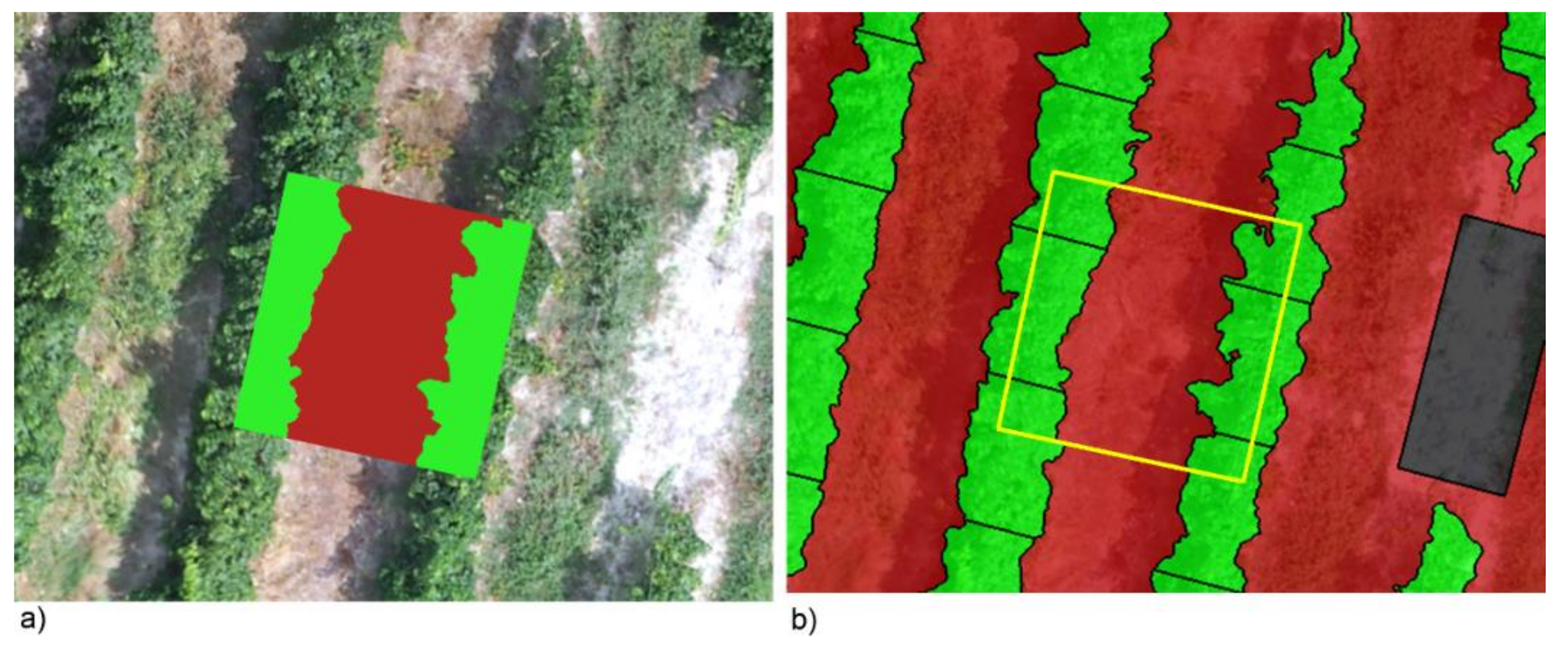
• Vine classification: A chessboard segmentation algorithm was used to segment the DSM in square objects of 0.5 m side size (Figure 3). The grid size was based on the common vine row width for trellis system that is around 0.7 m. Most of the objects that covered vine regions also included pixels of bare soil, making the DSM standard deviation (SD_DSM) within those objects very large. Thus, the objects with a SD_DSM greater than 0.15 m were classified as “vine candidates”. The 0.15 SD_DSM value was selected to be well suited for vine detection based on previous studies. The remaining objects were pre-classified as bare soil (Figure 3).
  The square objects that covered only vine regions had a low SD_DSM. To correctly classify them as “vine candidates”, the fact that they were surrounded by “vine candidates” was taken into account and implemented in the OBIA algorithm.
  Each individual “vine candidates” was automatically analyzed at the pixel level to refine the vine classification. Firstly, the “vine candidates” objects were segmented at the pixel size objects by using the chessboard segmentation process. Next, the algorithm classified every pixel as vineyard or bare soil by comparing their DSM value with that of the surrounding bare soil square (Figure 3). The 0.8 m value was used as suited threshold to accurately classify actual vine objects, based on previous studies, which also avoided misclassification of cover green as vine.
  The individual analysis of each “vine candidate” showed to be very suitable for vine classification, as only the surrounding soil altitude was taken into account for the discrimination, which could prevent errors due to field slope if the average soil altitude is considered instead. Moreover, using chessboard segmentation instead of the any other segmentation option, such as multi-resolution algorithm, decreases the computational time of the full process, because segmentation is by far the slowest task of the full OBIA procedure [21]. Thus, this configuration consisting of selecting DMS band as the reference for the segmentation instead of the spectral information, and the chessboard segmentation produced a notable increase in the processing speed without penalizing the segmentation accuracy [21].
• Gap detection in vine rows: Once the vines were classified, the gaps into the rows were detected by following four steps: (1) estimation of row orientation; (2) image gridding based on strips following the row orientation; (3) strip classification; and (4) detection of gaps. Firstly, a new level was created above the previous one to calculate the main orientation of the vines and then to generate a mesh of strips of 0.5 width size with the same orientation as the vine row. Then, a looping process was performed until all the strips were analyzed: the strip in the upper level with the higher percentage of vine objects in the lower one, as well as its neighbors strips, were classified as “vine row”; and continuously, the adjacent strips were classified as “no row” to simplify the process.

Finally, the strips classified as “vine row” in the upper level were segmented into 0.5 m length segments and compared to the lower level for gap detection, so that these segments were recognized as “gap” if no vine objects were placed in the lower level.

3.

Computing the vine geometric features: once the gaps into the row were identified, the vine rows were divided into 2 m length objects, which corresponded to each vine based on vine spacing. This parameter is user configurable to adapt the algorithm to different vine spacing. Before vine geometric feature calculation, the height of every pixel was individually obtained by comparing its DSM value (pixel height) to the average DSM value of the surrounding bare soil area. Then, the algorithm automatically calculated the geometric features (width, length and projected area, height and volume) of each vine, as follow: the highest height value of the pixels that composed the vine was selected as the vine height; and the volume was calculated by adding up the volumes (by multiplying the pixel areas and heights) of all the pixels corresponding to the vine. Finally, the geometric features of each vine, as well the identification and location, were automatically exported as vector (e.g., shapefile format) and table (e.g., Excel or ASCII format) files.

2.4. Validation

The validation of the vine classification and height estimation was carried out on the basis of a grid over the study fields, where 20 validation points were distributed and georeferenced during the flights in each field and year (Figure 4a,b).

2.4.1. Grapevine Classification and Gap Detection

A 2 × 2 m validation square was designed in every validation point, previously described, with the same orientation as the vine rows using ArcGis 10.0 (ESRI, Redlands, CA, USA) shapefiles to evaluate the performance of the grapevine classification. The very high spatial resolution of the orthomosaicked made possible to visually identify and manually classify the vine plants and soil in every designed square.

A confusion matrix was created to quantify the accuracy of the method by comparing the manual classification with the output of the automatic classification algorithm. The confusion matrix provided the overall accuracy (OA) of the classification (Equation (1)), which indicates the percentage of correctly classified area, and thus, the overall success of classification; and the Cohen’s Kappa index (Kc) (Equation (2)) that takes into account the possibility of the agreement occurring by chance. Information about the confusion matrix is shown in

Table 4. Error matrix schema for validation of vineyard classification.

		Classified Data
		Vineyard	No Vineyard
Manual classification	Vineyard	%VV	%VNV	TR1
	No vineyard	%NVV	%NVNV	TR2
		TC1	TC2	TR1 + TR2 = TC1 + TC2 = 100%

where: %V_V: percentage of data correctly classified as vineyard; %V_NV: percentage of data corresponding to vineyard wrongly classified as No vineyard; %NV_V: percentage of data wrongly classified as vineyard; %NV_NV: percentage of data correctly classified as No vineyard; TR1, TR2, TC1, and TC2 are the totals of row 1, row 2, column 1, and column 2, respectively.

.

$$\text{Overall Accuracy }\mathrm{OA}=\%{\mathrm{V}}_{\mathrm{V}}+\%{\mathrm{NV}}_{\mathrm{NV}}$$

(1)

$$\text{Kappa }Kc=\frac{p_o-p_c}{1-p_c}$$

(2)

where: Pc is the Proportion of chance agreement, $p_c =\frac{T_{C1}}{100}\times \frac{T_{R1}}{100}+\frac{T_{C2}}{100}\times \frac{T_{R2}}{100}$ and Po is the actual proportion of agreement, $p_o=\frac{\%V_V+\%N{V}_{NV}}{100}$.

For the validation of the gap detection, manual digitalization and length measurement of gaps were carried out in the orthomosaic. Thus, the on-ground gaps (real gap) were compared to the image OBIA process output, and the accuracy was measured by calculating true positive defined as real gaps correctly classified as gap; false positive refers to real vines wrongly classified as gaps; and false negative refers to real gaps wrongly classified as vines.

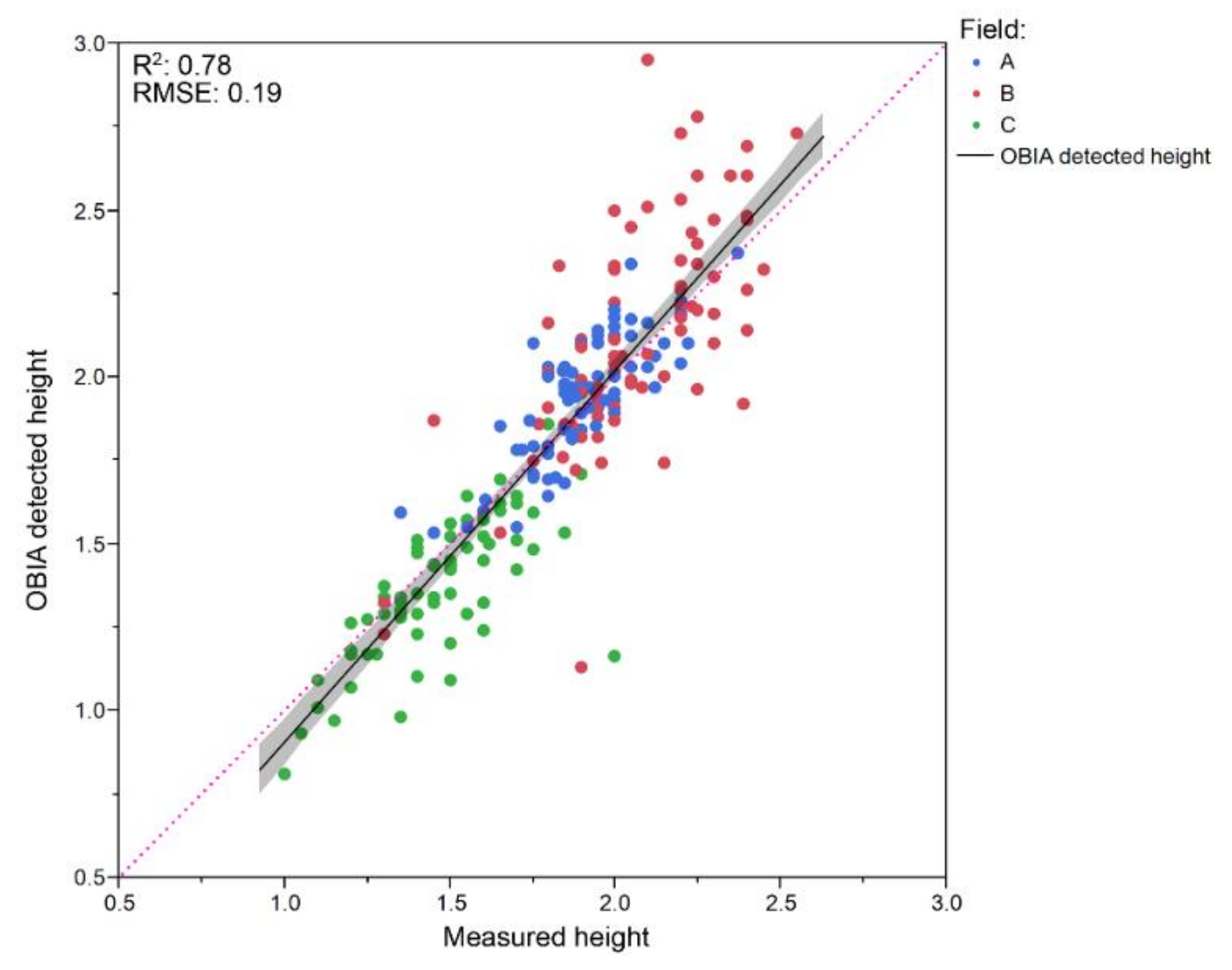
2.4.2. Grapevine Height

For height quantification, 40 true height data resulting of measuring on both sides of every validation point were taken in every field and date (Figure 4a,b). Each true data corresponding to grapevine height was photographed with the branch of the vine in front and the ruler included (Figure 4c). Then, the measured vine heights were compared to the height estimated by the OBIA algorithm. The coefficient of determination (R²) derived from a linear regression model and the root mean square error (RMSE) of this comparison were calculated using JMP software (SAS, Cary, NC, USA).

3. Results and Discussion

3.1. Vine Classification

The classification statistics obtained in the confusion matrix (OA and Kc) for every field and year are shown in

Table 5. Classification statistics (Overall accuracy and Kappa index) obtained in confusion matrix at every location and date.

Field	Date	Overall Accuracy (%)	Kappa
A	July	95.5	0.9
	September	95.4	0.9
B	July	95.2	0.9
	September	96.0	0.9
C	July	93.6	0.8
	September	96.1	0.7

. Overall Accuracy assessments varied slightly according to the location and year, providing OA values higher than 93.6% in all classifications, e.g., 95.5% in field A-July, and 96.0% and 96.1 in field B and field C in September, respectively. Therefore, OA values much greater than 85%—the minimum accepted value according to [38]—were recorded at all six cases analyzed, which indicated that the algorithm was able to accurately classify vines at different growth stages. An example of a validation frame is shown in Figure 5.

Regarding Kappa coefficient, values over 0.8 were achieved in most of the studied cases (e.g., 0.9 in field A-July and field B-September, and 0.8 in field C-July), which strongly indicates that these classifications are unlikely to have been obtained by chance alone [39]. Although the classification of field C-September did not achieve that high accurate value, the obtained kappa result of 0.7 pointed out a substantial classification agreement according to [39]. The lower Kappa results obtained in Field C could be due to irregular growth of vines, with many thin branches containing few leaves, which made the 3D canopy modelling more difficult. In fact, the low yield and irregular growth obtained last years in field C led the owner to uproot the entire field in winter 2015. Therefore, this fact highlights how crucial the accurate definition of DSM is for this procedure. Alternatively, the high accuracy obtained in this field based on OA contrasted with those lower Kappa values, and might be related to the fact that the Kappa statistic is more sensible to unbalanced classes, as the soil covered a greater portion of image than vines in this field.

Previous investigations have attempted to isolate vines using a spectral approach, for example Baluja et al. [9] used thresholding techniques to an inverse NDVI (Normalized Difference Vegetation Index) compute image to extract pure vine pixel. However, they detected problems with the inclusion of soil information or large loss of information, since determining the optimal threshold involved a compromise between retaining non-vine NDVI values and losing vine NDVI values. Similarly, Smit et al. [40] reported that achieving the optimal balance was a very difficult and inaccurate task and, consequently, thresholding on its own was not suitable for vine row classification. Comparatively, our results proved that less than 6.5% of soil was misclassified as vine (data not shown) using the DSM-based OBIA algorithm developed in this paper. Moreover, using those thresholding techniques for vine classification might generate inconsistent results due to shadows and inter-row cover crops. Puletti et al. [41] used the Red channel for identification of grapevine rows achieving acceptable accuracy values (lower than 87% of OA), however the inter-row spaces were not vegetation-covered. Therefore, the use of DSM in the vine classification is shown to be as a more accurate and efficient alternative to spectral approach, especially in the challenging spectral similarity scenario due to cover crops growing in the inter-rows.

In addition to the above, the OBIA algorithm developed was fully automatic compared to other approaches for vine classification that needed a manual touch-up to remove non-vine objects [29]; previous training of the classifier [10,12]; or manual delineation of vines [42]. Although some of these approaches achieved high level of accuracy, not much greater than that obtained in our work, they required user intervention and/or carried out the experiments in vineyard without cover crops growing in the inter-rows. In this way, the DSM-OBIA method offered a significant improvement compared to conventional classifiers, since it does not require any user intervention that makes the classification process time-efficient, reliable, and more accurate, removing errors from a subjective manual process [19].

3.2. Vine Gap Detection

Table 6. Results of the gap detection in vine rows. Percentages were calculated over the total length of gaps in the field.

Field	Date	True Positive (%)	False Positive (%)	False Negative (%)
A	July	100.0	1.12	0.0
	September	96.8	0.0	3.2
B	July	100.0	1.0	0.0
	September	100.0	6.0	0.0
C	July	100.0	0.0	0.0
	September	100.0	46.8	0.0

shows the classification results of gap detection obtained from the DSM-OBIA algorithm. The correct classification percentage (true positive) for each field and growth stage analyses was 100% except for field A-September, where the accuracy achieved was 96.8%. False negative that indicated wrongly classified gaps as vines only occurred in field A-September with a value of 3.2%, which proved the efficiency of the OBIA algorithm. Moreover, rates lower than 6% of vines were misclassified as gaps in fields A and B for both dates, and field C in July. However, higher rates of false positives were detected in field C-September due to the lower accuracy of vine 3D reconstruction, as explained in the previous section, which was even more prominent in September because of the harvest machinery activity.

This kind of information can be used for vineyard management, e.g., to target areas that need more specific attention [43]. Thus, false negatives might be more risky than false positives, as a problem that causes missing vine plants would be not detected. Delenne et al. [43] used images acquired from a manned ultra-light aircraft for vineyard delineation by using spectral approach, and they concluded that non-detection of missing vine plants could be due the spectral similarity of the grass under the row. According to our findings, the use of accurate DSM in the algorithm is crucial for gap detection, which was feasible using high UAV-imagery overlap and photogrammetric techniques.

3.3. Vine Height Quantification

Accuracy and graphical comparisons between the manually acquired and DSM-OBIA estimated vine heights for all fields and years are shown in Figure 6. The OBIA algorithm accurately estimated the plant height from the DSM of the vineyards achieving a very high correlation (R² = 0.78). A low RMSE of 0.19 was reported for this comparison, similar magnitude to that obtained in the detection of olive height using a visible-light camera attached to an UAV [20]. Moreover, most of the points were close to the 1:1 line with the points evenly scattered on either side of the line, which indicated an excellent fit of OBIA-estimated and measured height.

Analyzing the data by field and date (Figure 7), a better fit was obtained for each case reaching lower RMSE values for each one (<0.16), with the exception of field B-July, with independence of the growth stages, which demonstrated algorithm robustness. In a previous investigation, Burgos et al. [44] obtained similar results using image-based UAV technology for vine height detection, although an exhaustive validation was not carried out because of the lack of individual vine height, using average height of polygons instead, so this methodology remained non-validated at the individual vine level. In addition, [44] performed a flight plan with higher cost in time, consisting of perpendicular directions, which implies reducing the area analyzed due to the limited UAV autonomy; and generated a digital terrain model as well, thus increasing the computational time. Furthermore, Matese et al. [22] reported quite a discordance (0.50 m) between actual height and estimated height vines from UAV-based crop surface models due to the low resolution sensor used (1.3 MP), which caused a smoothing effect in the DSM generation. Accordingly, this issue could be solved employing higher spatial resolution images.

The lower accuracy observed for gap detection in field C-September contrasted with the accurate vine height detection (Table 6 and Figure 7, respectively). Despite limitations in the bottom of the vine canopy 3D reconstruction due to the weak canopy with sparse leaves, the top of them were correctly identified so that the OBIA algorithm was able to accurately detect the height of every vine. Consequently, the vine height detection is even effective when the 3D reconstruction of the bottom of the canopy is not very precise.

Based on our finding, the use of a DSM in the OBIA algorithm enabled the efficient assessment of vine height, and the development of DSM was feasible due to the high overlap and spatial resolution of UAV-imagery. To the best of our knowledge, OBIA-based technology has not yet been applied to automatically estimate vine height, and subsequently, to validate the procedure using individual ground truth data. In this context, some authors have estimated vine height by using photogrammetric point clouds from UAV imagery, such as Weiss and Baret [8] and Ballesteros et al. [5]. However manual intervention was needed in both approaches, which would make the process less time-efficient and less accurate due to errors from a subjective manual process [19]. Moreover, they pointed out that no exhaustive validation was carried out, which was a pending challenge. Therefore, the experiments carried out in this paper overcame both limitations of manual intervention and precise validation.

The DSM-OBIA process hence developed is useful for trellis system, one of the most widely used training systems around the word. However more training systems are routinely employed in vineyard fields depending on the production objective (wine quality, yield), the cost of the system, climate, topography, vine vigor, vine variety, and mechanization requirements, among others. Thereby, the OBIA algorithm could be adapted to those training system characteristics. In addition, this approach was based on the DSM, which allowed for isolation of the vine from the bare soil and cover crops, which is considered a major issue in vineyard characterization [8]. Cover crops are a common practice widely used in vineyard as a management tool to maintain the optimal vine growth and fruit development, as well as controlling the excess grapevine shoot vigor. For these purposes, cover crops are kept at low height. Although it hardly ever occurs, the cover crops could achieve a higher altitude than the vines, making it difficult to isolate the vine. Accordingly, it could be solved by adding the orthomosaic to the OBIA algorithm, and thus combining textural, spectral, topological, or contextual information to separate vine and cover crops.

3.4. Potential Algorithm Result Applications

The technological combination of UAV imagery and the DSM-OBIA algorithm herein developed enables the rapid and accurate vineyard characterization by identifying, isolating, and extracting geometric features of every vine at several growth stages. This accurate methodology has multiple implications for PV purposes, for example, it could be used to automatically mask soil and cover crops pixels and extract information of every vine from multispectral imagery for disease detection [10]; or thermal imagery for assessment the vineyard water status [45], as requested by [9,46].

Vine volume could be efficiently estimated from the accurate area classification and vine height detection, by multiplying the height and area of every pixel that compose the vine canopy. This approach would leave those few leaves bellow the basal level of the vineyard canopy without computing, since they are difficult to identify. Alternatively, on-the-go soil sensing systems, as a terrestrial laser scanner, have shown potential to estimate vine volume for precision applications, as spraying application [47]. However, these systems are slower than UAV technology and enable one to only take one vineyard side information. Therefore, a combination of mobile terrestrial sensors and OBIA-UAV technology could be conducted in further research to evaluate the performance of both approaches in vine volume quantification.

The algorithm output can be automatically exported both as table files (

Table 7. A sample of the output data file delivered by the OBIA algorithm for vine of field A-September.

X Center	Y Center	Length (m)	Width (m)	Area (m2)	Vine Max Height (m)	Vine Mean Height (m)	Vine Volume (m3)
290,909.63	4,615,191.17	1.36	0.48	0.51	2.02	1.49	0.76
290,909.85	4,615,192.23	2.06	1.41	1.93	2.13	1.33	2.56
…	…	…	…	…	…	…	…
290,910.55	4,615,194.39	2.05	1.21	1.32	2.22	1.53	2.02
290,918.60	4,615,225.30	2.06	1.74	2.35	2.22	1.72	4.05
290,919.09	4,615,227.23	2.14	1.65	2.15	2.18	1.54	3.31
290,919.60	4,615,229.19	2.03	1.37	1.46	2.00	1.41	2.06
290,920.12	4,615,231.14	2.19	1.63	2.13	2.00	1.40	2.99

) and vector files, i.e., geo-referenced maps with the locations and dimensions of every vine (Figure 8), thus showing the spatial variability of the vineyard, a crucial key for precision viticulture [1]. These geo-referenced maps with the dimensions of every vine could be useful to identify less vigor or size areas that require special attention, as well as being the basis for designing a site-specific management program [10,48]. For example, Figure 8 showed that vines in field C had much lower volume than fields A and B, which was indicative of the low vigor that led growers to uproot the field.

This technology has been proven at two growth stages, and its use in a multi-temporal approach could open new opportunities to monitor vine status and progress at the field scale, as an efficient and accurate alternative to the arduous and inconsistent manual measurements on the ground. For example, Figure 9 shows the distribution of height, area, and volume of a vine row at the two dates studied (July and September) that corresponded to different growth stages. Segment length is a user-configurable parameter for the algorithm output, and for this example 0.10 m was selected to catch in detail the impact of the harvesting machinery. Specifically, this Figure showed that vine area decreased from July to September in a higher range, around 40%, than that of the other geometric characteristics, which could be directly due to the harvest, as the machinery activity causes the berries to fall off the stem, as well as leaves and other debris that may have fallen from the vines along with the fruit. The height parameter showed a slight decrease of around 6%, since the machinery affects the upper part of the vines much less. As the volume is calculated directly from the area and height of the vine, it decreased in an intermediate range of 30%. Canopy monitoring throughout the growing cycle could help growers with multiple purposes, such as identifying biotic stress, irrigation deficit or nutrient status. In addition, this approach would help to address the goal of improving prediction models that connect the vine geometric characteristics with the vineyard yield, which is a complex issue that depends on a large number of factors [21].

4. Conclusions

A robust and fully automatic OBIA algorithm was developed for the 3D characterization of the vineyard fields, including vine classification, height estimation, and gap detection, from UAV-imagery. Using photogrammetric-based DSM as input in the algorithm, the misclassification due to spectral similarity between vines and green-cover growing in the inter-rows was avoided. The DSM-OBIA model was tested in three commercial vineyards at two different growth stages using images acquired with a low-cost camera onboard an UAV. The algorithm accurately detected the area and height of the vines, and the existence of gaps. Moreover, the developed OBIA algorithm is self-adaptive to different crop-field conditions, as row orientation, row and vine spacing, field slope, inter-row cover crops, or grapevine dimensions. This fully automatic process, without previous training or user intervention, is an important asset that makes this procedure time-efficient, reliable and more accurate, removing the potential errors inherent to a manual process.

In addition, the algorithm output can be exported as geo-referenced maps with the locations and dimensions of every vine, thus showing the spatial variability of the vineyard, a crucial key for precision management. Volume of the vine canopy can be estimated from the area and height of vines, which could be considered another potentiality of this methodology. Thereby, the procedure developed, based on ultra-high-spatial resolution DSMs and the OBIA algorithm, has shown to be a valuable tool for the accurate characterization of the vines that has important implications for the adoption of Precision Viticulture. Thus, for instance, it could help growers to identify less vigor or size areas that require special attention, monitor the vine growth, determine the proper moment to harvest, or to evaluate the effect different trimming treatments in the grapevine canopy structure.

References

1. Bramley, R.G.V.; Hamilton, R.P. Understanding variability in winegrape production systems. Aust. J. Grape Wine Res. 2004, 10, 32–45. [Google Scholar] [CrossRef]
2. Arnó, J.; Casasnovas, J.A.M.; Dasi, M.R.; Rosell, J.R. Precision viticulture. Research topics, challenges and opportunities in site-specific vineyard management. Span. J. Agric. Res. 2009, 7, 779–790. [Google Scholar] [CrossRef]
3. Schieffer, J.; Dillon, C. The economic and environmental impacts of precision agriculture and interactions with agro-environmental policy. Precis. Agric. 2014, 16, 46–61. [Google Scholar] [CrossRef]
4. Tey, Y.S.; Brindal, M. Factors influencing the adoption of precision agricultural technologies: A review for policy implications. Precis. Agric. 2012, 13, 713–730. [Google Scholar] [CrossRef]
5. Ballesteros, R.; Ortega, J.F.; Hernández, D.; Moreno, M.Á. Characterization of Vitis vinifera L. Canopy Using Unmanned Aerial Vehicle-Based Remote Sensing and Photogrammetry Techniques. Am. J. Enol. Vitic. 2015. [Google Scholar] [CrossRef]
6. Hall, A.; Lamb, D.W.; Holzapfel, B.; Louis, J. Optical remote sensing applications in viticulture—A review. Aust. J. Grape Wine Res. 2002, 8, 36–47. [Google Scholar] [CrossRef]
7. Johnson, L.F.; Roczen, D.E.; Youkhana, S.K.; Nemani, R.R.; Bosch, D.F. Mapping Vineyard leaf area with multispectral satellite imagery. Comput. Electron. Agric. 2003, 38, 33–44. [Google Scholar] [CrossRef]
8. Weiss, M.; Baret, F. Using 3D Point Clouds Derived from UAV RGB Imagery to Describe Vineyard 3D Macro-Structure. Remote Sens. 2017, 9, 111. [Google Scholar] [CrossRef]
9. Baluja, J.; Diago, M.P.; Balda, P.; Zorer, R.; Meggio, F.; Morales, F.; Tardaguila, J. Assessment of vineyard water status variability by thermal and multispectral imagery using an Unmanned Aerial Vehicle (UAV). Irrig. Sci. 2012, 30, 511–522. [Google Scholar] [CrossRef]
10. Albetis, J.; Duthoit, S.; Guttler, F.; Jacquin, A.; Goulard, M.; Poilvé, H.; Féret, J.-B.; Dedieu, G. Detection of Flavescence dorée Grapevine Disease Using Unmanned Aerial Vehicle (UAV) Multispectral Imagery. Remote Sens. 2017, 9, 308. [Google Scholar] [CrossRef]
11. Mathews, A.J.; Jensen, J.L.R. Visualizing and Quantifying Vineyard Canopy LAI Using an Unmanned Aerial Vehicle (UAV) Collected High Density Structure from Motion Point Cloud. Remote Sens. 2013, 5, 2164–2183. [Google Scholar] [CrossRef]
12. Poblete-Echeverría, C.; Olmedo, G.F.; Ingram, B.; Bardeen, M. Detection and Segmentation of Vine Canopy in Ultra-High Spatial Resolution RGB Imagery Obtained from Unmanned Aerial Vehicle (UAV): A Case Study in a Commercial Vineyard. Remote Sens. 2017, 9, 268. [Google Scholar] [CrossRef]
13. Rey-Caramés, C.; Diago, M.P.; Martín, M.P.; Lobo, A.; Tardaguila, J. Using RPAS Multi-Spectral Imagery to Characterise Vigour, Leaf Development, Yield Components and Berry Composition Variability within a Vineyard. Remote Sens. 2015, 7, 14458–14481. [Google Scholar] [CrossRef]
14. Nex, F.; Remondino, F. UAV for 3D mapping applications: A review. Appl. Geomat. 2013, 6, 1–15. [Google Scholar] [CrossRef]
15. Mancini, F.; Dubbini, M.; Gattelli, M.; Stecchi, M.; Fabbri, S.; Gabbianelli, G. Using Unmanned Aerial Vehicles (UAV) for High-Resolution Reconstruction of Topography: The Structure from Motion Approach on Coastal Environments. Remote Sens. 2013, 5, 6880–6898. [Google Scholar] [CrossRef] [Green Version]
16. Rosnell, T.; Honkavaara, E. Point cloud generation from Aerial image data acquired by a quadrocopter type micro unmanned aerial vehicle and a digital still camera. Sensors 2012, 12, 453–480. [Google Scholar] [CrossRef] [PubMed]
17. Geipel, J.; Link, J.; Claupein, W. Combined spectral and spatial modeling of corn yield based on aerial images and crop surface models acquired with an unmanned aircraft system. Remote Sens. 2014, 6, 10335–10355. [Google Scholar] [CrossRef]
18. Bendig, J.; Bolten, A.; Bennertz, S.; Broscheit, J.; Eichfuss, S.; Bareth, G. Estimating Biomass of Barley Using Crop Surface Models (CSMs) Derived from UAV-Based RGB Imaging. Remote Sens. 2014, 6, 10395–10412. [Google Scholar] [CrossRef]
19. De Castro, A.I.; Torres-Sánchez, J.; Peña, J.M.; Jiménez-Brenes, F.M.; Csillik, O.; López-Granados, F. An Automatic Random Forest-OBIA Algorithm for Early Weed Mapping between and within Crop Rows Using UAV Imagery. Remote Sens. 2018, 10, 285. [Google Scholar] [CrossRef]
20. Torres-Sánchez, J.; López-Granados, F.; Serrano, N.; Arquero, O.; Peña, J.M. High-Throughput 3-D Monitoring of Agricultural-Tree Plantations with Unmanned Aerial Vehicle (UAV) Technology. PLoS ONE 2015, 10, e0130479. [Google Scholar] [CrossRef] [PubMed]
21. Jiménez-Brenes, F.M.; López-Granados, F.; de Castro, A.I.; Torres-Sánchez, J.; Serrano, N.; Peña, J.M. Quantifying pruning impacts on olive tree architecture and annual canopy growth by using UAV-based 3D modelling. Plant Methods 2017, 13, 55. [Google Scholar] [CrossRef] [PubMed]
22. Matese, A.; Gennaro, S.F.D.; Berton, A. Assessment of a canopy height model (CHM) in a vineyard using UAV-based multispectral imaging. Int. J. Remote Sens. 2017, 38, 2150–2160. [Google Scholar] [CrossRef]
23. Blaschke, T.; Hay, G.J.; Kelly, M.; Lang, S.; Hofmann, P.; Addink, E.; Queiroz Feitosa, R.; van der Meer, F.; van der Werff, H.; van Coillie, F.; et al. Geographic Object-Based Image Analysis—Towards a new paradigm. ISPRS J. Photogramm. 2014, 87, 180–191. [Google Scholar] [CrossRef] [PubMed]
24. Peña, J.M.; Torres-Sánchez, J.; de Castro, A.I.; Kelly, M.; López-Granados, F. Weed Mapping in Early-Season Maize Fields Using Object-Based Analysis of Unmanned Aerial Vehicle (UAV) Images. PLoS ONE 2013, 8, e77151. [Google Scholar] [CrossRef] [PubMed]
25. Souza, C.H.W.; Lamparelli, R.A.C.; Rocha, J.V.; Magalhães, P.S.G. Mapping skips in sugarcane fields using object-based analysis of unmanned aerial vehicle (UAV) images. Comput. Electron. Agric. 2017, 143, 49–56. [Google Scholar] [CrossRef]
26. Castillejo-González, I.L.; Peña-Barragán, J.M.; Jurado-Expósito, M.; Mesas-Carrascosa, F.J.; López-Granados, F. Evaluation of pixel- and object-based approaches for mapping wild oat (Avena sterilis) weed patches in wheat fields using QuickBird imagery for site-specific management. Eur. J. Agron. 2014, 59, 57–66. [Google Scholar] [CrossRef]
27. Mathews, A.J. Object-based spatiotemporal analysis of vine canopy vigor using an inexpensive unmanned aerial vehicle remote sensing system. J. Appl. Remote Sens. 2014, 8, 085199. [Google Scholar] [CrossRef]
28. López-Granados, F.; Torres-Sánchez, J.; Castro, A.-I.D.; Serrano-Pérez, A.; Mesas-Carrascosa, F.-J.; Peña, J.-M. Object-based early monitoring of a grass weed in a grass crop using high resolution UAV imagery. Agron. Sustain. Dev. 2016, 36, 67. [Google Scholar] [CrossRef]
29. Laliberte, A.S.; Goforth, M.A.; Steele, C.M.; Rango, A. Multispectral Remote Sensing from Unmanned Aircraft: Image Processing Workflows and Applications for Rangeland Environments. Remote Sens. 2011, 3, 2529–2551. [Google Scholar] [CrossRef]
30. Laliberte, A.S.; Rango, A.; Herrick, J.E.; Fredrickson, E.L.; Burkett, L. An object-based image analysis approach for determining fractional cover of senescent and green vegetation with digital plot photography. J. Arid Environ. 2007, 69, 1–14. [Google Scholar] [CrossRef]
31. Hellesen, T.; Matikainen, L. An Object-Based Approach for Mapping Shrub and Tree Cover on Grassland Habitats by Use of LiDAR and CIR Orthoimages. Remote Sens. 2013, 5, 558–583. [Google Scholar] [CrossRef]
32. Van Den Eeckhaut, M.; Kerle, N.; Poesen, J.; Hervás, J. Object-oriented identification of forested landslides with derivatives of single pulse LiDAR data. Geomorphology 2012, 173–174, 30–42. [Google Scholar] [CrossRef]
33. Franklin, S.E.; Ahmed, O.S. Deciduous tree species classification using object-based analysis and machine learning with unmanned aerial vehicle multispectral data. Int. J. Remote Sens. 2017, 1–10. [Google Scholar] [CrossRef]
34. Meier, U. BBCH Monograph: Growth Stages for Mono- and Dicotyledonous Plants, 2nd ed.; Blackwell Wissenschafts-Verlag: Berlin, Germany, 2001. [Google Scholar]
35. AESA. Aerial Work—Legal Framework. Available online: http://www.seguridadaerea.gob.es/LANG_EN/cias_empresas/trabajos/rpas/marco/default.aspx (accessed on 6 November 2017).
36. Torres-Sánchez, J.; López-Granados, F.; Borra-Serrano, I.; Peña, J.M. Assessing UAV-collected image overlap influence on computation time and digital surface model accuracy in olive orchards. Precis. Agric. 2018, 19, 115–133. [Google Scholar] [CrossRef]
37. Dandois, J.P.; Ellis, E.C. High spatial resolution three-dimensional mapping of vegetation spectral dynamics using computer vision. Remote Sens. Environ. 2013, 136, 259–276. [Google Scholar] [CrossRef]
38. Foody, G.M. Status of land cover classification accuracy assessment. Remote Sens. Environ. 2002, 80, 185–201. [Google Scholar] [CrossRef]
39. Landis, J.R.; Koch, G.G. The measurement of observer agreement for categorical data. Biometrics 1977, 33, 159–174. [Google Scholar] [CrossRef] [PubMed]
40. Smit, J.L.; Sithole, G.; Strever, A.E. Vine signal extraction: An application of remote sensing in precision viticulture. S. Afr. J. Enol. Vitic. 2016, 31, 65–74. [Google Scholar] [CrossRef]
41. Puletti, N.; Perria, R.; Storchi, P. Unsupervised classification of very high remotely sensed images for grapevine rows detection. Eur. J. Remote Sens. 2014, 47, 45–54. [Google Scholar] [CrossRef]
42. Matese, A.; Toscano, P.; Di Gennaro, S.F.; Genesio, L.; Vaccari, F.P.; Primicerio, J.; Belli, C.; Zaldei, A.; Bianconi, R.; Gioli, B. Intercomparison of UAV, Aircraft and Satellite Remote Sensing Platforms for Precision Viticulture. Remote Sens. 2015, 7, 2971–2990. [Google Scholar] [CrossRef]
43. Delenne, C.; Durrieu, S.; Rabatel, G.; Deshayes, M. From pixel to vine parcel: A complete methodology for vineyard delineation and characterization using remote-sensing data. Comput. Electron. Agric. 2010, 70, 78–83. [Google Scholar] [CrossRef] [Green Version]
44. Burgos, S.; Mota, M.; Noll, D.; Cannelle, B. Use of Very High-Resolution Airborne Images to Analyse 3D Canopy Architecture of a Vineyard. Int. Arch. Photogramm. Remote Sens. Spat. Inf. Sci. 2015, 40, 399. [Google Scholar] [CrossRef]
45. Santesteban, L.G.; Di Gennaro, S.F.; Herrero-Langreo, A.; Miranda, C.; Royo, J.B.; Matese, A. High-resolution UAV-based thermal imaging to estimate the instantaneous and seasonal variability of plant water status within a vineyard. Agric. Water Manag. 2016, 183, 49–59. [Google Scholar] [CrossRef]
46. Espinoza, C.Z.; Khot, L.R.; Sankaran, S.; Jacoby, P.W. High Resolution Multispectral and Thermal Remote Sensing-Based Water Stress Assessment in Subsurface Irrigated Grapevines. Remote Sens. 2017, 9, 961. [Google Scholar] [CrossRef]
47. Llorens, J.; Gil, E.; Llop, J.; Escolà, A. Variable rate dosing in precision viticulture: Use of electronic devices to improve application efficiency. Crop Prot. 2010, 29, 239–248. [Google Scholar] [CrossRef] [Green Version]
48. Hall, A.; Lamb, D.W.; Holzapfel, B.P.; Louis, J.P. Within-season temporal variation in correlations between vineyard canopy and winegrape composition and yield. Precis. Agric. 2010, 12, 103–117. [Google Scholar] [CrossRef]
Figure 1. Images of the studied fields at different growth stages: (a) inter-row cover crop growing in Field C in July; (b) the UAV flying over Field B; and (c,d) comparison between the field situations (green cover crops, vines, and bare soil) between July and September in Field B.
Remotesensing 10 00584 g001
Figure 2. A partial view of the 3-D Point Cloud for the vineyard field A in July, which was produced by the photogrammetric processing of the remote images taken with the UAV.
Remotesensing 10 00584 g002
Figure 3. Flowchart and graphical examples of the Object Based Image Analysis (OBIA) procedure outputs for automatic vine characterization.
Remotesensing 10 00584 g003
Figure 4. Experimental set for validating the results: (a) validation point grid in Field A on July; (b) a vector squares used for classification validation (yellow points indicate the positions of 40 true height data, and the white square is the artificial target placed in the field); (c) measurement of the vine height.
Remotesensing 10 00584 g004
Figure 5. Example of a 2 × 2 validation frame in field A-July: (a) manually classified orthomosaicked image (R-G-B composition); (b) DSM-OBIA-based classification.
Remotesensing 10 00584 g005
Figure 6. Graphic comparing DSM-OBIA estimated and vine height for all data corresponding to the three fields and both dates (July and September). The root mean square error (RMSE) and correlation coefficient (R2) derived from the regression fit are included (p < 0.0001). The solid line is the fitted linear function and the pink dashed line represents the 1:1 line.
Remotesensing 10 00584 g006
Figure 7. DSM-OBIA detected height vs. measured vine height divided by field and date. The root mean square error (RMSE) derived from the regression fit are included (p < 0.0001). The solid line is the fitted linear function and the pink dashed lines represent the 1:1 line.
Remotesensing 10 00584 g007
Figure 8. Four-level representation of the estimated vine canopy volume as computed on the three fields in July, from left to right: From left to right: Field A, Field B, and Field C. In the axes, coordinate system UTM zone 31 N, datum WGS84.
Remotesensing 10 00584 g008
Figure 9. Height, area, and volume values in two dates (July and September, corresponding to different growth stages) from the left side to the row. Every data corresponded to 0.10 m length segments of the vine row.
Remotesensing 10 00584 g009