Article

Topography and Three-Dimensional Structure Can Estimate Tree Diversity along a Tropical Elevational Gradient in Costa Rica

1
Department of Geography, University of California, Los Angeles, CA 90095, USA
2
Jet Propulsion Laboratory, California Institute of Technology, Pasadena, CA 91109, USA
3
Institute of Environment and Sustainability, University of California, Los Angeles, CA 90095, USA
4
Department of Biology, University of Missouri-St. Louis, St. Louis, MO 63121, USA
5
Organization for Tropical Studies, Puerto Viejo de Sarapiquí, Heredia 41001, Costa Rica
6
Department of Statistics, University of California, Los Angeles, CA 90095, USA
*
Author to whom correspondence should be addressed.
Remote Sens. 2018, 10(4), 629; https://doi.org/10.3390/rs10040629
Submission received: 25 February 2018 / Revised: 7 April 2018 / Accepted: 12 April 2018 / Published: 18 April 2018
(This article belongs to the Special Issue Remote Sensing of Tropical Forest Biodiversity)

Abstract

:
This research seeks to understand how tree species richness and diversity relates to field data (1-ha plots) on forest structure (stems, basal area) and lidar derived data on topography and three-dimensional forest structure along an elevational gradient in Braulio Carrillo National Park, Costa Rica. In 2016 we calculated tree species richness and diversity indices for twenty 1-ha plots located along a gradient ranging from 56 to 2814 m in elevation. Field inventory data were combined with large footprint (20 m) airborne lidar data over plots in 2005, in order to quantify variations in topography and three-dimensional structure across plots and landscapes. A distinct pattern revealing an increase in species’ richness and the Shannon diversity index was observed in correlation with increasing elevation, up to about 600 m; beyond that, at higher elevations, a decrease was observed. Stem density and basal area both peaked at the 2800 m site, with a mini-peak at 600 m, and were both negatively associated with species richness and diversity. Species richness and diversity were negatively correlated with elevation, while the two tallest relative height metrics (rh100, rh75) derived from lidar were both significantly positively correlated with species richness and diversity. The best lidar-derived topographical and three-dimensional forest structural models showed a strong relationship with the Shannon diversity index (r2 = 0.941, p < 0.01), with ten predictors; conversely, the best species richness model was weaker (r2 = 0.599, p < 0.01), with two predictors. We realize that our high r² has to be interpreted with caution due to possible overfitting, since we had so few ground plots in which to develop the relationship with the numerous topographical and structural explanatory variables. However, this is still an interesting analysis, even with the issue of overfitting. To reduce issues with overfitting we used ridge regression, which acted as a regularization method, shrinking coefficients in order to decrease their variability and multicollinearity. This study is unique because it uses paired 1-ha plot and airborne lidar data over a tropical elevation gradient, and suggests potential for mapping species richness and diversity across elevational gradients in tropical montane ecosystems using topography and relative height metrics from spaceborne lidar with greater spatial coverage (e.g., GEDI).

Graphical Abstract

1. Introduction

Tropical forests are experiencing high rates of deforestation and degradation; this has had in a strongly adverse impact on biodiversity and ecosystem services [1,2,3]. In recent years, the international community has recognized the loss of diversity—and the associated impact upon ecological functions and services—as a key threat to the sustainability of tropical ecosystems [2]. Quantifying patterns and understanding the processes that maintain species diversity across tropical landscapes are considered among the ten most challenging problems that require spatial data from combined ground and remote observations to resolve [4]. Tropical montane forests are of particular interest because of their high diversity, the complexity of their landscapes, the intensity of degradation from anthropogenic forces, and their vulnerability to changing climate.
Patterns of diversity along elevational gradients in tropical montane forests have been the subject of many studies [5,6,7,8]. Diversity along elevational gradients was initially believed to decline linearly from the warmer lowlands to the cooler highlands, analogous to patterns exhibited by increasing latitude [8,9,10,11,12]. However, recent tropical montane studies that examine the full extent of elevational gradients show a pattern characterized by a mid-elevation diversity peak of trees, epiphytes, and mammals [5,8,12,13,14,15,16,17,18,19,20,21,22]. Species diversity is hypothesized to be greatest midway up the gradient, at an ecotone type environment, with species intermingling from both lower and higher elevations [6,19,23,24]. However, the structure of the forest may also be a key mechanism for diversity patterns, and may also explain why there are more species at mid-elevations. In particular, field data suggests that stem density and biomass may be associated with diversity along elevation gradients, and new technologies such as lidar are available to examine the micro-topography and three-dimensional structure of tropical forests [25,26,27].
Several aspects of forest structure data, including stem density, basal area, and aboveground biomass, are generally collected in the field and may be associated with tree diversity [28,29]. In general, sites with higher numbers of individuals per unit area, e.g., higher stem density, tend to have more species [6,13,17,18,30,31,32,33,34]. A similar pattern has also been noted for basal area and biomass of forests, with the high diversity in areas with the highest basal area [28,35,36]. However, there have been a number of studies in lowland rainforests that have reported only weak relationships between diversity and basal area/biomass, as just a few large trees may contain much of the biomass [37,38].
Canopy and understory structural variations and topographical metrics have been associated with patterns of diversity in tropical lowlands, and can be quantified through the use of lidar remote sensing [37,39]. Lidar can provide waveforms of the returned energy from relatively small to large footprints, over large areas. Prior research has found that lidar waveform data closely matched field-collected vertical canopy profiles in the lowland forest [40,41]. If there is a reasonable relationship between the lidar-derived topography, and three-dimensional structure of a forest stand and plot data are representative of the landscape, it should be feasible to predict tree diversity across an entire area covered by a lidar swath. Utilizing lidar technology over larger areas may be assessed more quickly than ground-collected data alone, and may help to pinpoint critical areas for conservation priorities [42,43,44].
There are a number of theoretical and empirical reasons why lidar metrics on topography and three-dimensional structure should be associated with patterns of diversity. The topographic variables of elevation, slope, and aspect have been reported to show varying levels of predictive power for diversity; these can easily be quantified with lidar [24,28,45]. In particular, steep slopes generally result in areas with less soil development, lower levels of soil nutrients, and less water retention, and hence, less diversity than in valleys or on mild slopes [24,28,37,45,46]. In addition, it has also been hypothesized that aspect, or the orientation of a site, may be associated with diversity with areas with less direct sun light. Such areas may maintain higher water holding potential, and thus support greater species richness [37,47]. Studies in tropical forests have clearly shown that the development of high and structurally complex canopies results in greater species richness [37,48]. In particular, the mean and standard deviation of tree or canopy height have been associated with high levels of diversity in tropical forests, with taller trees and more heterogeneity in the canopy permitting a wider niche for other tree species to persist [39,49,50]. Recent studies have also shown that upper canopy variability is correlated with increased species richness among trees (>1 cm dbh), possibly due to partitioning of light resources [37]. In particular, metrics on canopy height and heterogeneity have been able to predict 25% of the variation of species richness for trees ≥10 cm dbh in lowland rainforests [39].
This research seeks to assess how tree species richness and diversity changes along a Neotropical elevational gradient within Braulio Carrillo National Park in Costa Rica. This research has three primary research objectives. First, we test if species richness and diversity and the mid-elevation peak is associated with forest structure metrics (stems, basal area) collected in 1-ha plots in the field. Second, we test whether topographical and forest structural metrics derived from lidar were associated with tree species richness and diversity within 1-ha plots. Third, we examined if lidar-derived topographical and three-dimensional structural metrics within plots are representative of the overall landscape of Braulio Carrillo National Park.

2. Materials and Methods
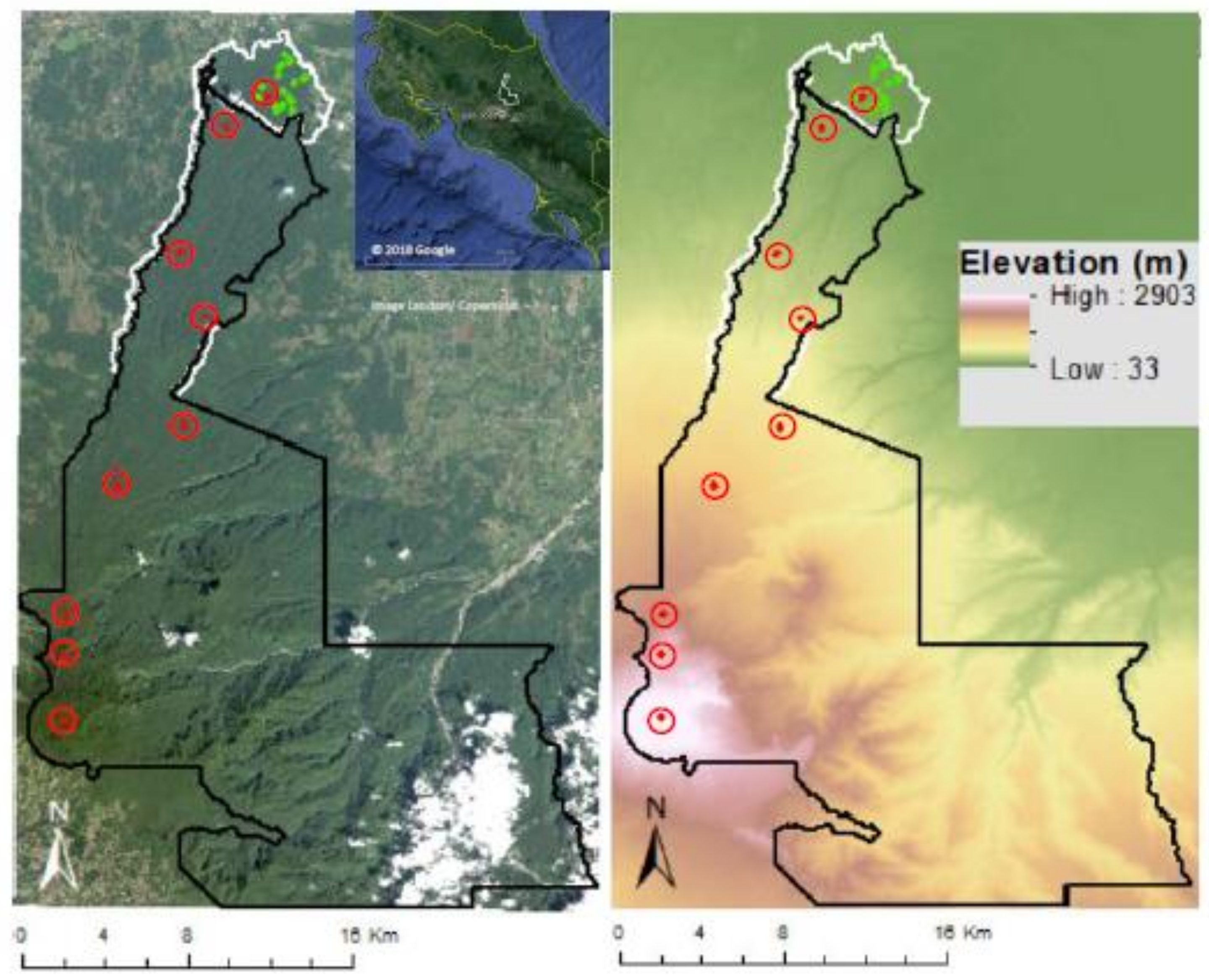
2.1. Study Area

This research was conducted along a unique tropical forest elevational gradient in Costa Rica, with 1-ha plots spanning from within the La Selva Biological Station at 56 m above sea level (m.a.s.l) up to 2814 m.a.s.l. in Braulio Carrillo National Park (BCNP). This elevational gradient, protected by a National Park, is quite unique for Central America, spanning several ecoregions, from lowlands to high elevation cloud forest, and providing the conditions for high species turnover and diversity [51]. The lowland forest in this region has an average annual rainfall of ~4000 mm, with ~9000 mm at mid-elevations and ~3000 mm at the peak [6,22,52]. The average temperature is 26 °C in the lowlands; temperatures decrease with increased elevation, down to ~10 °C at the peak [28]. Soil types vary over the region, but all are influenced by the past activity of the Barva Volcano; parent materials of basaltic and andesitic lavas from the Plio-Pleistocene age are common along the gradient, with more agglomerate tuff-like soil at high elevations [53]. Due to volcanic activity, the soils are younger and have endured less weathering near the peak of the Barva Volcano [6,53]. Besides the uniqueness of the protected area extending over multiple life zones, this area is also special because it offers paired field and airborne lidar data over a tropical elevation gradient, which few other places in the world offer [40,52]. We use the term ‘landscape’ when we refer to the area within Braulio Carrillo National Park, which is a mountainous area surrounded by lowlands covered in agricultural land. Here, we are only concerned with the landscape of the mountainous and forested protected area of Braulio Carrillo National Park and La Selva Biological Station, covered by the lidar dataset.

2.2. Field Data

Vegetation surveys were conducted along the gradient within BCNP for 20 1-ha plots ranging from 56 m.a.s.l. to 2814 m.a.s.l. (Figure 1). Tree diameter at breast height (DBH, 1.3 m) was measured using a fabric diameter tape +/−1 mm resolution for all trees ≥10 cm DBH. Species were determined in field and identified using herbarium vouchers. Nine of the 1-ha plots were from a collaborative effort of Conservational International’s TEAM Project [54], and 11 1-ha plots at <120 m.a.s.l. at the La Selva Biological Station, as part of the Carbono project [28]. For both datasets, the survey data from 2011 was used to assess patterns of tree species’ richness, diversity and structural characteristics (stem density and basal area) along this elevational gradient. The data used in this study is currently available online, at http://www.teamnetwork.org/ [54].

2.3. Lidar Remote Sensing

Lidar data were used to assess topographic variation (elevation, slope, and aspect), as well as three-dimensional forest structure metrics (canopy height and understory variation) across the majority of BCNP and within the 1-ha plots (Table 1). We used NASA’s Land, Vegetation, and Ice (LVIS) sensor, a medium altitude airborne laser altimeter system, operating up to 10 km above ground, with a varying footprint, but usually flown in a medium resolution with circular footprints of 10–30 m in diameter. LVIS was flown over BCNP in 2005 between March 22nd–30th on the DOE King Air B-200 platform [43,55,56]. Within each footprint, lidar measures distance from the instrument to the surfaces below, resulting in several signal returns, effectively capturing canopy height with the first returns and a digital elevation model (DEM) with the last. The waveform outputs can help to derive canopy heights, vertical relative height metrics (rh metrics), and topographic features, relative to the WGS-84 ellipsoid [43]. The DEM from the last return of the LVIS signal was used to calculate elevation, slope in degrees, and aspect which was converted to cos(aspect). For three-dimensional structure, the LVIS waveform was segmented into quartiles of energy, also known as relative height metrics (rh100, rh75, rh50, and rh25), to quantify three-dimensional forest structure [55]. These relative height metrics allow for the assessment of forest structure from the upper canopy (rh100), the canopy (rh75) the sub-canopy (rh50) and the understory (rh25) at the 1-ha plot level. Past research has found that these four metrics provide enough information from the waveform to study forest structure [26,27,39,43].
While there is a temporal discrepancy between the LVIS data collection and more recent field collections, we did compare 2005 field data to the 2016 data for a few plots that were available, and these displayed similar values of diversity across all life forms; we are assuming the natural growth and treefall occurrence over the interim years. In addition, from multiple visits to the sites, we do not believe that the structure or levels of species richness have changed significantly between the time periods.

2.4. Data Analysis

Species richness and the Shannon diversity index were calculated for each plot [7,57]. Species richness was defined as the number of tree species ≥10 cm dbh per ha, while the Shannon diversity index is a metric of diversity that also includes information on evenness or the proportion of individuals of each species, so it also takes into account the community structure as a whole (S1) [58,59]. The mean and standard deviation of topographic metrics (elevation, slope, aspect) and three-dimensional structure metrics (rh25, rh50, rh75, rh100) were calculated at the plot level. Pearson correlations and regression analyses in R were used to determine the relationship between species richness and diversity and field data on forest structure (stem density and basal area from plots), and lidar-derived metrics (topographical metrics and forest three-dimensional structure within the plots).
In order to extrapolate the plot-level data to the landscape, we fit linear models that predict species richness and diversity from field- and lidar-derived topographical and three-dimensional forest structure metrics. For each response variable, we used the leaps package in R to optimize the multiple linear regression model by fitting an exhaustive set of models—including all combinations of predictor variables—and choosing the model that minimized the Bayesian Information Content (BIC) [57,60]. In addition to using BIC as a measure of performance on each fitted model, cross-validation was also performed to optimize the number of predictors included in the multiple linear regression, by estimating the testing Mean Squared Error (MSE) of optimal models with each number of predictors. Because many predictors were included in the multiple linear regressions compared to the number of observations in the data, our model was very flexible. We constrained this flexibility in order to reduce overfitting by using ridge regression.
Ridge regression acted as a regularization method, shrinking coefficients in order to decrease their variability and multicollinearity. The linear regression and ridge regression models were compared using 5-fold cross-validation to estimate the testing MSE, in order to judge the extrapolation quality of our field data derived model [61,62]. We compared the mean and standard deviation of topography and three-dimensional structure metric from the field plots with the landscape based on lidar derived metrics. We calculated canopy heights across 100 m bins of elevation, which we refer to as landscape data. Plot data was paired with lidar data, and a Shapiro-Wilk normality test showed that the differences between them were approximately normally distributed. Paired t-tests were performed between plot and landscape data to identify if topography (slope and aspect) and three-dimensional forest structure (rh100, rh75, rh50, rh25) from the plots were significantly different from landscape data.

3. Results

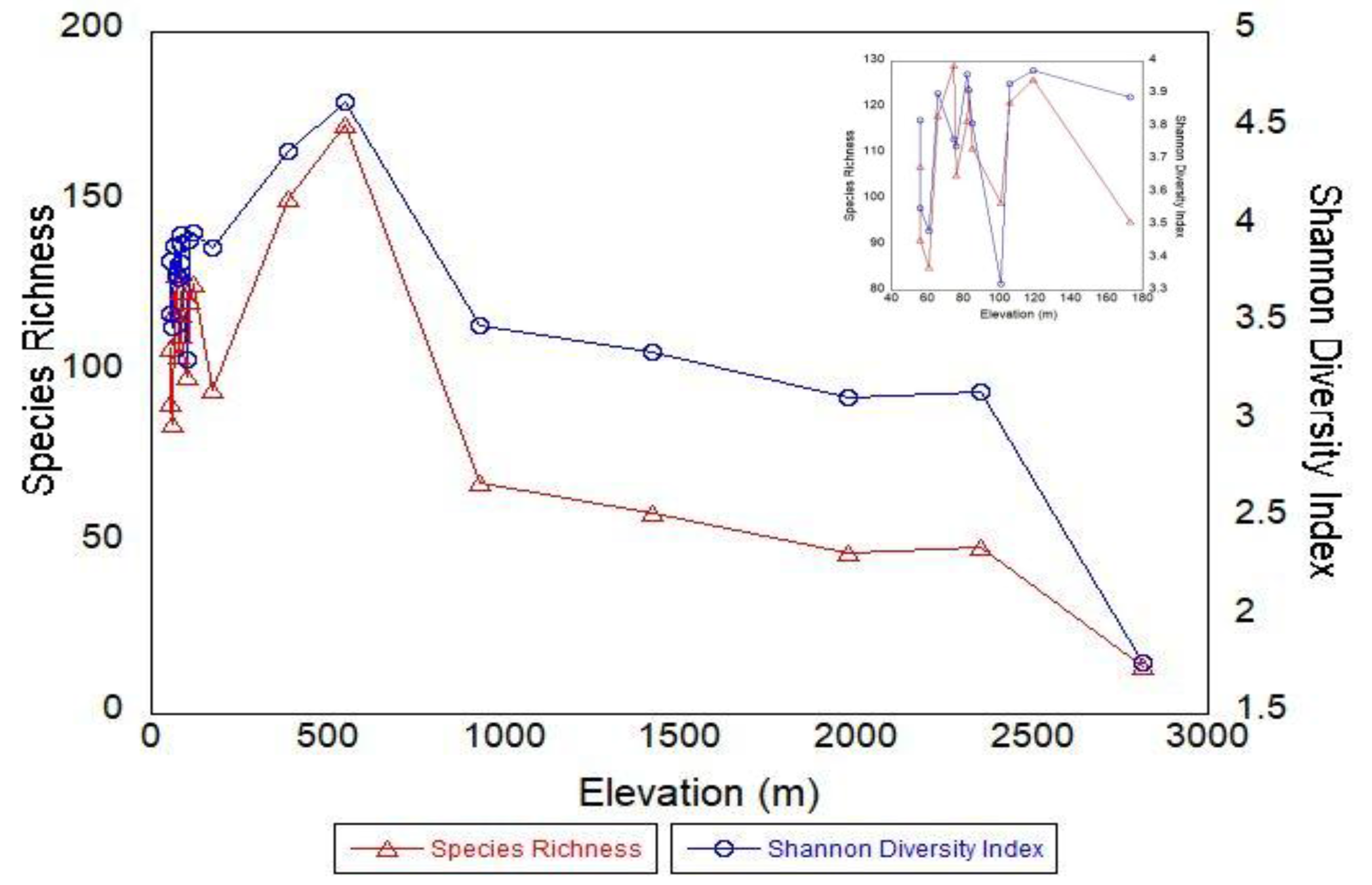
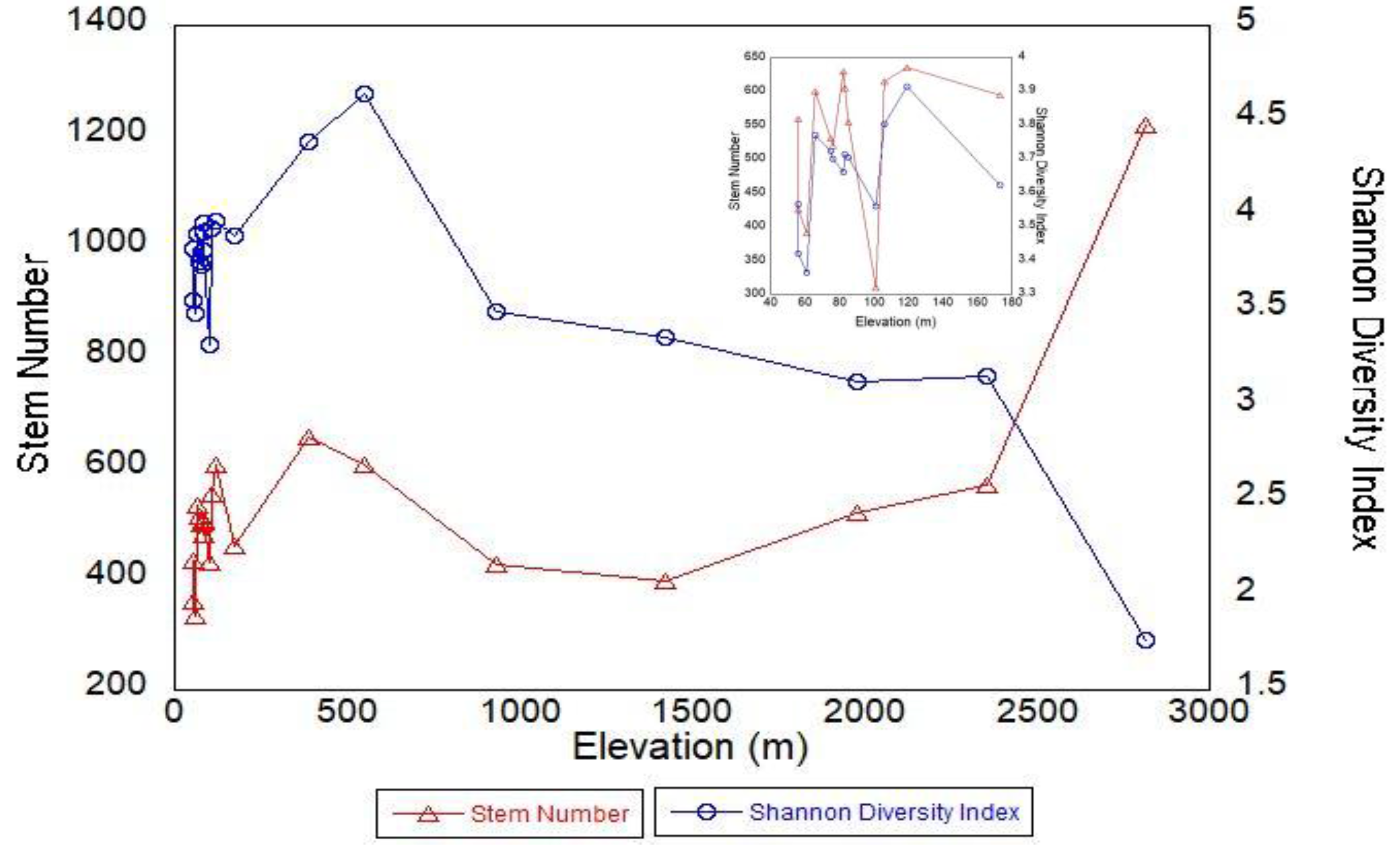
3.1. Species Richness, Diversity, and Forest Structure from Plots

There were 403 identified tree species ≥10 cm dbh in the 20 1-ha plots, representing 87 different families. Tree species richness and diversity changed in a non-linear fashion along the montane gradient (Figure 2); species richness (178 sp.) and Shannon diversity (4.64) both peaked at the plot located at 552 m elevation, VB3 (Table 1).
From the lowest elevation sites, species richness and diversity steadily increased up to 552 m, then declined, with an exceptionally large decline after the 2355 m plot. This 2355 m plot had a species richness of 49 and a Shannon diversity index of 3.2, and the highest elevation site (2813 m) had a species richness of 13 and a Shannon index of 1.77 (Table 1, Figure 2).
Stem density increased from 221 stems per hectare at the 56 m plot to 657 stems at 386 m; it then decreased to 606 stems at 552 m, and 397 stems at 1425 m, and exceptionally increased to 1221 stems at the 2814 m plot (Table 1). At lower elevations, basal area had a pattern similar to stem density, with a peak at the 106 m plot (27.9 m2) and 552 m (27.5 m2); it then decreased before a slight increase at 1425 m. The two highest plots, 2355 m and 2814 m, had the highest basal area along the elevational gradients (35.8 m2 and 66.2 m2 respectively).
Species richness was not significantly correlated with stem density and basal area; however, Shannon diversity was significantly negatively correlated with stem density (Figure 3) and basal area (Table 2). The results of Pearson correlation tests between each of these response variables of species richness and diversity with stem density were r = −0.272, p < 0.25 and r = −0.517, p < 0.02, respectively. The results of Pearson correlation tests between each of these response variables and basal area were r = −0.550 p < 0.002 and r = −0.739, p < 0.001, respectively (Table 2).

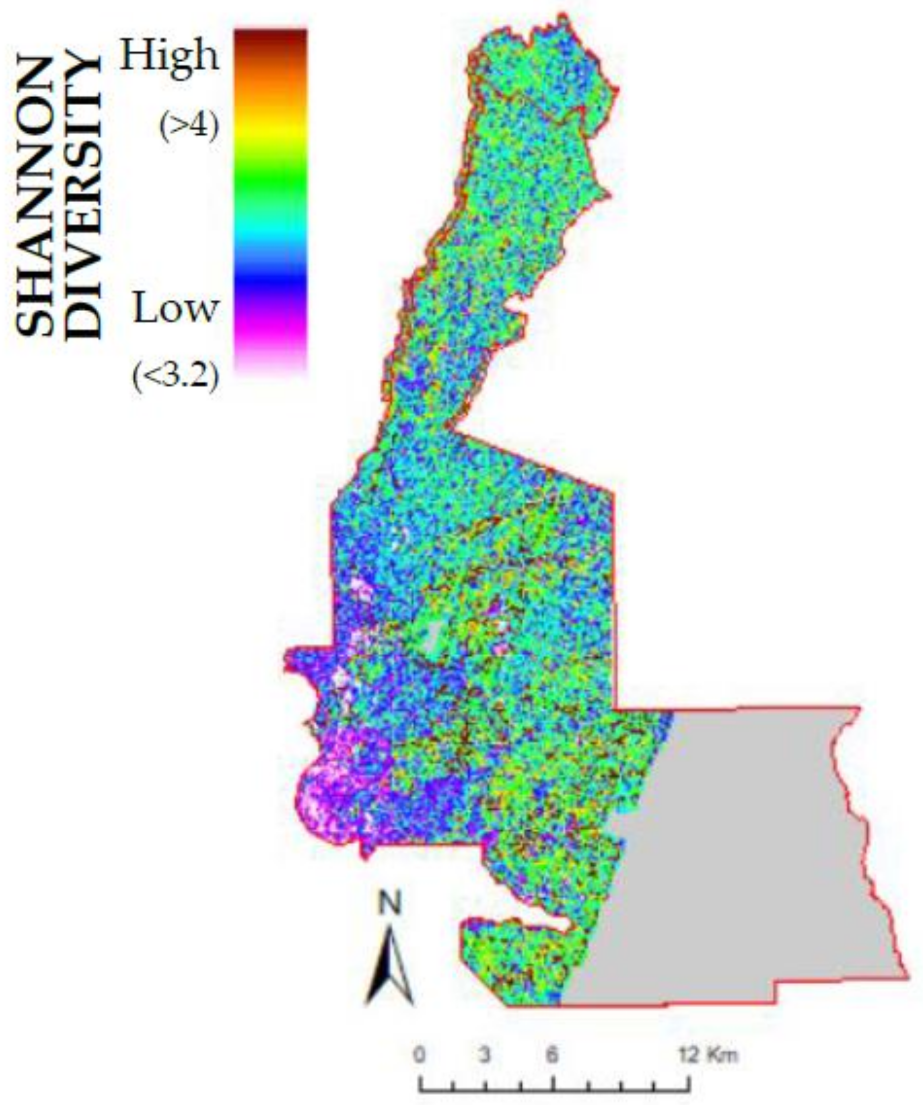
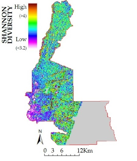
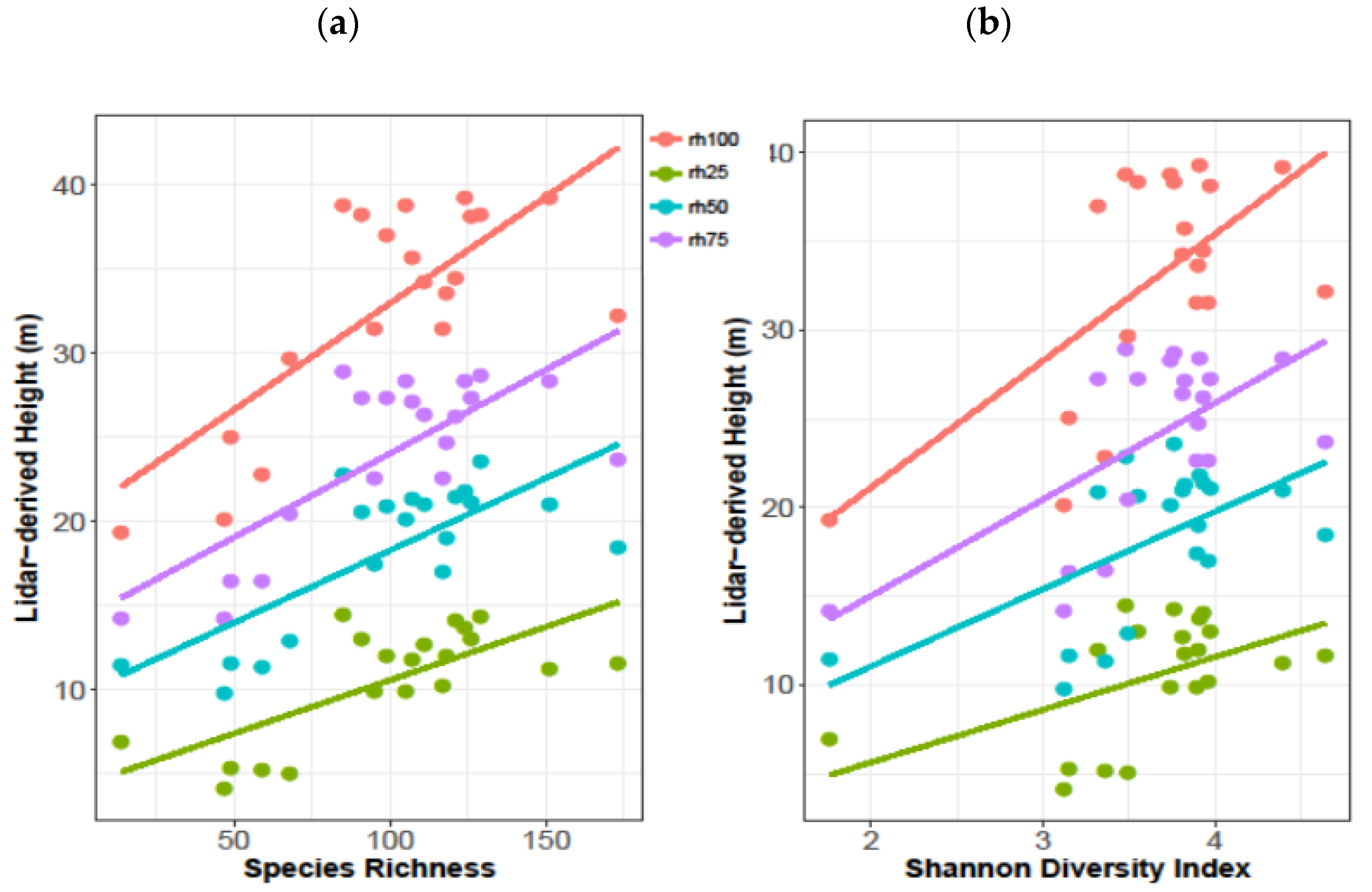
3.2. Lidar Metrics and Species Richness and Diversity

Topographic and three-dimensional structure were correlated with metrics of species richness and the Shannon diversity index (Table 2). Lidar metrics on topographic variables were more closely correlated with Shannon diversity than species richness. For the topographic variables, elevation was significantly correlated with species richness and diversity. For height metrics, species richness was correlated with the top two canopy height metrics, rh100 and rh75, and the standard deviation of the understory, while diversity was correlated with the top three canopy height metrics and the standard deviation of the upper canopy. The lidar metrics derived from the quartiles of the lidar waveform were found to have a relatively linear relationship with tree species richness and diversity, particularly for lower rh metrics (Figure 4a,b). The multivariate regressions focused on the use of topographic and three-dimensional structure to predict species richness and the Shannon diversity index. Using best subset selection, the species richness model with optimal BIC included two predictors, rh100 and rh25 SD, and the model with the second-lowest BIC included three predictors, adding aspect to the model (Table 3). These models had r2 values of 0.494 and 0.557, respectively. Applying this method to the multivariate regression predicting the Shannon diversity index selected an optimal model, with 10 predictors (Table 4, Figure 4).
Regularization was performed on models for species richness and Shannon diversity index. We used a shrinkage parameter lambda, that minimizes the residual sum of squares, plus an L2 constraint, meaning that the shrinkage parameter lambda is the coefficient of an added term that is the sum of the squared coefficients. This constraint encourages the beta coefficient estimates to become smaller than they would be using ordinary least squares regression. Using L2 constraint, ridge regression optimized the shrinkage parameter lambda and yielded sets of coefficients (S2) with 14 degrees of freedom. This was done using the package glmnet; the value of our optimized lambda was 0.04037017 [63]. Comparison of multiple linear regression subset selection and regularization methods was performed using 5-fold cross validation to estimate the mean squared error on testing data. Cross validation on multiple linear regression subset selection models for species richness and Shannon diversity yielded average validation set mean squared errors of 572.2 and 0.02 respectively, while cross validation on models using ridge regression yielded higher mean squared errors of 2628.8 and 0.39 (Table 5). Overall, the reduced multiple linear regression models formed using best subset selection (10 predictors for diversity, 2 predictors for species richness) performed the best (Figure 5).
This map of Shannon Diversity Index over the Braulio Carrillo National Park area exemplifies the extrapolation capabilities, when using combined ground and airborne data (Figure 5). We see that the highest elevation areas (South West corner of BCNP, bottom left of map) tend to have the lowest species diversity. We obviously do not see a visible mid-elevation bulge of diversity in the raster image, but there are more pixels that are mid- to high-diversity in the center of BCNP, and in the mid-elevation region depicted in the digital elevation model of Figure 1b. There are some homogenous clumps of pixels in the middle of BCNP, which are likely artifacts caused by sharp changes in elevation, which can cause errors with lidar collection [39]. The southeast portion of BCNP was not covered by the lidar sensor, so we masked it out of the extrapolation.

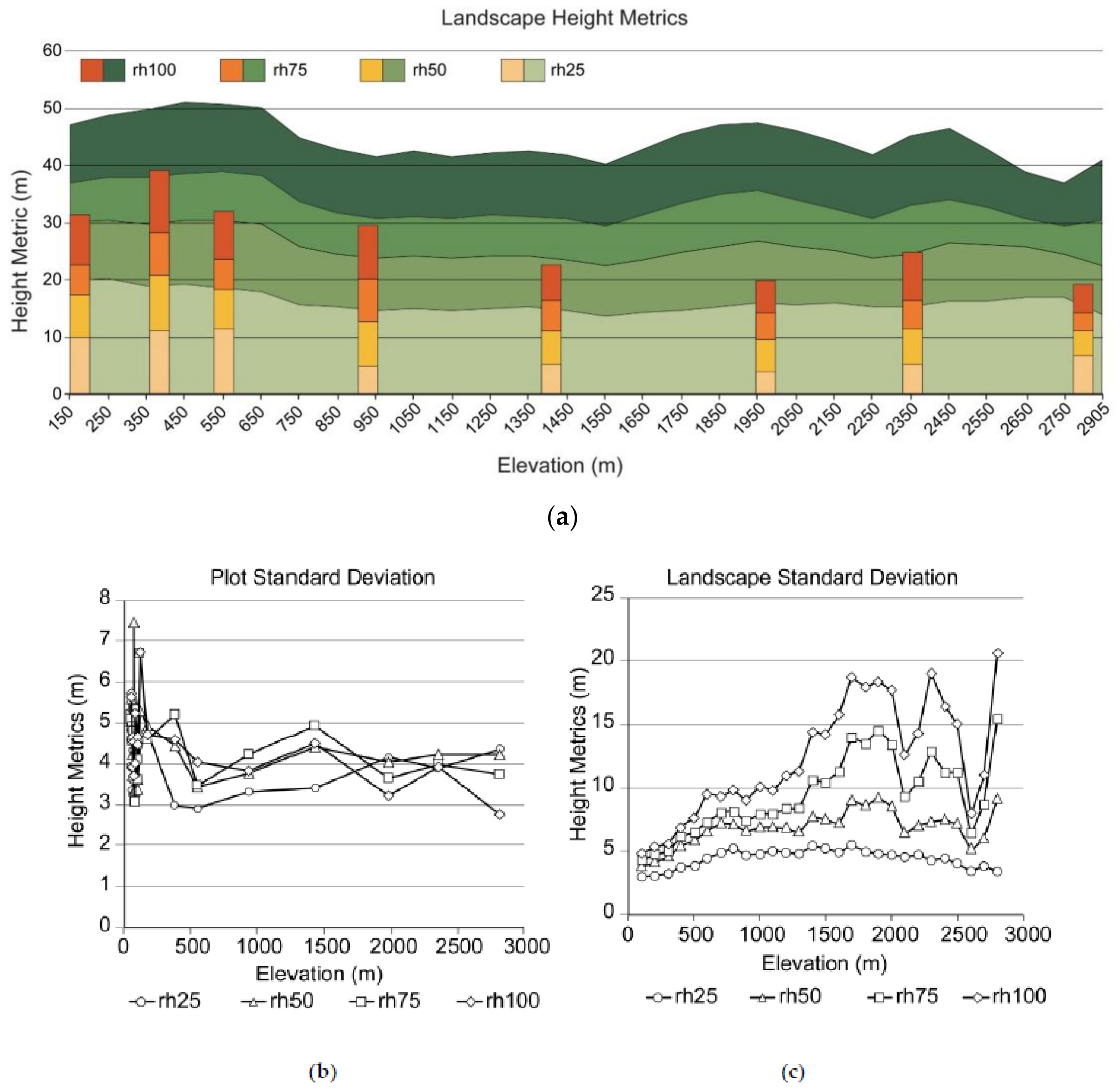
3.3. Plot and Landscape Data

Plot level lidar data on topography and three-dimensional structure were compared to landscape-level data in 100 m bins, in order to see if the lidar-derived topographic and height data from the plots was representative of the landscape as a whole. Slope and aspect from the plots were not significantly different than the landscape (p = 0.161, p = 0.818 respectively). The mean canopy heights were correlated for the plots and landscapes (p < 0.05) (Figure 6a); however, the canopy heights were significantly taller across the landscape than plots (p < 0.01). There was a significant difference in standard deviation of plot and lidar derived landscape data (p < 0.01). The standard deviation from plots were relatively similar across the elevational gradient (generally within 2 m), while the standard deviation at the landscape scale showed wide variation in rh100 and rh75 and a clear increase in standard deviation with elevation (Figure 6b,c), with exceptions of the two highest elevation sites 2355 and 2814 m.

4. Discussion

4.1. Species Richness and Diversity

Overall, patterns of species richness and diversity decreased with elevation, with a peak at 552 m of the total 2906 m of elevation of the mountaintop. This peak in diversity had an overlap of species from both the higher and lower elevation plots, and had the highest number of shared species with the other sites, as determined through a test of beta diversity (Figure 7). This seemingly skewed bulge may also have to do with the geometry of a mountain or mountain range, as higher elevations cover less area as they come to a peak, compared with larger geographic areas at mid-elevations. According to the species-area relationship, larger geographic areas should support a greater variety of species [7]. As elevation increases in simple montane environments, the total area within zones of elevation decreases in accordance with basic geometry, which would support the idea that higher elevations would have fewer species. However, the ruggedness of terrain can influence the surface area in certain bands of elevation, making the area effectively larger [7].
The mid-elevation bulge of tree diversity has been observed across continents and biomes in the Himalayas [17,18,20], Costa Rica [22], Mexico [14,15], Peru [64], and Ethiopia [21]. Although a monotonic linear decrease of diversity has been reported for many studies, it appears that many of these studies often do not sample the entire gradient, instead presenting a truncated form of the mid-gradient bulge pattern [12]. These results suggest that if the entire elevational extent is not sampled, the overall patterns may not be correctly identified, and an incorrect assumption might be made regarding linear decreases in plant diversity with elevation change; this may cause the display of a mid-elevation bulge, as we found on our mountain gradient.

4.2. Forest Structure from Field Measurements

Patterns in species richness and diversity were not associated with increased stem density and basal area. When comparing the number of stems and basal area directly to the Shannon diversity index, we found that the three highest elevation plots (1976, 1355, and 2814 m) had a distinctly different pattern than the other sites. While most sites had a positive relationship between diversity and higher numbers of stems/larger basal area, the three high elevation plots displayed the opposite pattern. They were relatively species poor, but had higher stem density, particularly at the 2814 m site, where there were twice as many stems within 1-ha. Thus, stem number and basal area from plot data alone may not be used to predict tree species diversity at different elevations. This can be due to a variety of factors, including that our plot locations may not be representative of the gradient as a whole. Without replicates, we cannot know whether certain factors are solely due to the aspect of the plot locations.

4.3. Topography and Three Dimensional Structure from Lidar

Lidar metrics on topography and three-dimensional structure were associated with both species richness and diversity. We expected that high elevation, steep slopes, and slopes that receive the most solar radiation would have low species richness and diversity, while high forest canopies with high canopy heterogeneity would have greater species richness and diversity. The topographic metrics of elevation were the most important in this study. Although mean and standard deviation of slope and aspect was not correlated with species richness or diversity, these topography metrics improved diversity models, and combined, could explain more of the variance than the three-dimensional structure metrics. High forest canopies and understories had the highest species richness and diversity, while high canopy heterogeneity—as measured by the standard deviation—have greater diversity. This suggests that high canopies with greater variation allow for more species to persist, resulting in higher diversity.

4.4. Plots vs. Landscape

We found that forest canopy height structure displayed a non-linear relationship along the gradient, with various peaks of canopy height. At the landscape scale, when we calculated canopy height across the same elevation as plots in 100 m bins, we found two peaks of canopy height—the highest around 500 m and a secondary peak at 1900 m, with maximum heights of 52 and 45 m respectively. The height metrics extracted from just within the field plots resulted in similar patterns across mean height metrics as those of the landscape scale, although landscape values were generally taller than plots. This can have implications when we use the relationship developed from the plots to the landscape. At the plot level, we found the standard deviation of the height metrics was highest at the lower elevation sites; however, the landscape scale clearly had higher standard deviations of the height metrics increasing with elevation. This high variation in the forest canopy, and difference between the landscape and plot level analysis, could be due to higher disturbance in highlands versus lowlands, which could also affect the diversity and observed shifts in composition [22]. These results differ slightly from findings on the same gradient from a study published in 1996, with ground-measured height displaying peaks of height at 300 m and 1750 m elevation, with heights of 47 m and 31 m respectively [6]. This is also different from what has been found in the Andes, where tree height and biomass decrease with elevation [29]. However, tree height does not always simply decrease with elevation in the Neotropics. In terms of plot locations, they were placed for field surveys, and the lidar was collected years later. If the lidar was collected before setting up the plots, the sampling could have changed, and we may have obtained slightly different results. With the lidar data, we would have had better knowledge of the topography and structural variations, and preferentially chosen certain slopes or elevations based on features seen in that data. We recommend that non-linear models be tested in the future (e.g., below and above 552 m), along with other biodiversity metrics—such as butterfly and bird diversity—that are available for some of the plots in this study.

4.5. Modeling Diversity and Species Richness

Lidar metrics of topography and three-dimensional structure can be used to predict tree diversity and species richness to a lesser extent along elevational gradients, in areas without ground data. There have been a number of studies that have examined tree species richness and diversity from plots, and spectral sensors and indices (e.g., NDVI), over tropical forests; however, these have only been able to explain between 30% and 40% of the variation in tropical tree species richness [65,66,67]. Active remote sensing, such as airborne radar and small footprint lidar, have been able to explain between 25% to 44% of the variation in tree species richness (10 cm dbh) within tropical forests [37,39,68]. Our results from large footprint lidar can explain 94% of the variation in tree diversity, and 49% of the variation in tree species richness. This suggests that large footprint lidar can be used to quantify tree diversity and species richness in regions with 1-ha plots, and may be able to estimate diversity and species richness along elevational gradients of forests in the tropics. For diversity, a number of topography and height metrics best explain tree diversity patterns, and these should be tested in other regions. However, since we tested a number of variables (n = 20) that have been associated with tree diversity from the literature (and observed that there was not a linear relationship with diversity), fewer variables and non-linear models should also be tested in the future. We realize that many variables, with so few plots, can cause an issue with overfitting. It is difficult to avoid overfitting in our situation, because the data collection is limited to small sample sizes, coupled with the presence of a lot of noise in real life. However, this is still an interesting analysis, even with the issue of overfitting. For species richness, the overall canopy height (rh100) and the heterogeneity in the understory (standard deviation of rh25) may be the two best metrics associated with tree species richness at 1-ha for tree 10 cm dbh. Tree species richness may be the best variable to test in the future using air and spaceborne lidar data, since the two metrics are easy to calculate, extrapolate, and because they explain nearly half of the tree species richness. We would expect to find canopy height and understory structure to be correlated with diversity for other tropical forests along elevational gradients. Indeed, Guo et al. [8] identified peaks of diversity in the tropics, and these peaks may be directly related to canopy height and topographic complexity.

4.6. Future Research

Active remote sensing systems like lidar sensors are becoming increasingly popular, making new forest analyses possible. Lidar has the ability to collect tree height and other aspects of forest structure and topography that are important for accurate measurements and monitoring of forest inventory information [25,69,70,71]. LVIS lidar has been collected along elevational gradients for a number of forests across the United States; however, the coverage over tropical forests remains limited to Costa Rica (Land, Vegetation, And Ice Sensor (LVIS) [55]). Globally comparative canopy height data (e.g., relative height) are available from the Geoscience Laser Altimeter System (GLAS) sensor, and have been found to correlate with results from LVIS [72,73]. Thus, it should be possible to compare topography and three-dimensional structure data from GLAS tracks to tropical field plots, in order to test results from our research, and possibly map diversity and species richness. NASA’s Global Ecosystem Dynamics Investigation Lidar (GEDI) will provide a global dataset in the future on canopy structure, similar to GLAS and LVIS, but with a footprints of 25 m. This dataset may be used to maps patterns of vegetation structure using relative height metrics and diversity across elevational gradients in the tropics, and at larger scales than the LVIS airborne lidar used in this study.

5. Conclusions

We examined tree species richness and diversity from field data (20 1-ha plots) on forest structure (stems, basal area) and large footprint lidar derived data on topography and three-dimensional forest structure along an elevational gradient in Brauilo Carrillo, Costa Rica. This study is special because airborne lidar data, with paired field collections, is rare over tropical elevation gradients. Slope and aspect from the plots seemed to be representative of the surrounding landscape of the national park; however, the canopy height was significantly taller across the landscape, and there were differences in standard deviation of lidar derived plot and landscape data. Species richness and the Shannon diversity index showed a distinct pattern of increasing up to about 600 m elevation, and then decreasing at higher elevations. Stem density and basal area were negatively associated with species richness and diversity, with both peaking at about 2800 m. Elevation was negatively correlated with species richness and diversity, while the two tallest relative height metrics (rh100, rh75) derived from lidar were both significantly positively correlated with species richness and diversity. The best lidar-derived topographical and three-dimensional forest structural models showed a strong relationship with the Shannon diversity index (r2 = 0.941, p < 0.01), with ten predictors, while the best species richness model was weaker (r2 = 0.599, p < 0.01), with two predictors (rh100, standard deviation of rh25). The resultant map of Shannon Diversity shows the lowest diversity at the highest elevations in the southwest of BCNP, with higher pixel values of diversity in mid-elevation areas. This suggests a potential for mapping species richness and diversity across elevational gradients in tropical montane ecosystems using spaceborne lidar.

Supplementary Materials

The following are available online at https://www.mdpi.com/2072-4292/10/4/629/s1.

Acknowledgments

The authors benefited from multiple workshops organized through the University of Washington, as part of the National Science Foundation Dimensions of Biodiversity Distributed Graduate Seminar Series, made possible through a National Science Foundation Dimensions of Biodiversity grant (1050680) to Sandy Andelman and Julia Parrish. The TEAM (Tropical Ecology Assessment & Monitoring) network and a joint NASA-Organization for Tropical Studies (OTS) project funded much of the field data collection. The forest inventory data were provided by the Tropical Ecology Assessment and Monitoring (TEAM) Network, collaboration between Conservation International, the Missouri Botanical Garden, the Smithsonian Institution, and the Wildlife Conservation Society, and partially funded by these institutions, the Gordon and Betty Moore Foundation, and other donors. Forest inventory plots research at La Selva was also supported by the NSF LTREB program, most recently by NSF 1357177 to D.B. Clark (PI, Co-PIs D.A. Clark and J.R. Kellner). We thank the staff of the La Selva Biological Station for logistic support and the National Park Service and the National Ministry of the Environment for permission to conduct this research. The authors would also like to thank the key contributions of the TEAM and NASA parabiologists, including Marcos Molina, Gilbert Hurtado, Juan Gabriel Huertas Reyes, and Wagner Corella, who conducted the field surveys under challenging conditions. We would like to thank three reviewers for their time and their thoughtful comments and suggestions.

Author Contributions

C.R. did the analysis and writing; S.S. provided guidance and funding; D.C. provided access to the vegetation surveys he had set up years prior, as well as guidance in the field; J.H.A. aided with the setup of many of the field expeditions and helped to maintain the plots for years; A.H. aided with some statistical calculations; T.G. guided throughout the process and edited the manuscript and figures many times.

Conflicts of Interest

The authors declare no conflict of interest. The founding sponsors had no role in the design of the study; in the collection, analyses, or interpretation of data; in the writing of the manuscript, and in the decision to publish the results.

References

  1. Chapin, F.S.; Zavaleta, E.S.; Eviner, V.T.; Naylor, R.L.; Vitousek, P.M.; Reynolds, H.L.; Hooper, D.U.; Lavorel, S.; Sala, O.E.; Hobbie, S.E.; et al. Consequences of changing biodiversity. Nature 2000, 405, 234–242. [Google Scholar] [CrossRef] [PubMed]
  2. Jantz, S.M.; Barker, B.; Brooks, T.M.; Chini, L.P.; Huang, Q.; Moore, R.M.; Noel, J.; Hurtt, G.C. Future habitat loss and extinctions driven by land-use change in biodiversity hotspots under four scenarios of climate-change mitigation. Conserv. Biol. 2015, 29, 1122–1131. [Google Scholar] [CrossRef] [PubMed]
  3. Olivares, I.; Svenning, J.-C.; van Bodegom, P.M.; Balslev, H. Effects of warming and drought on the vegetation and plant diversity in the Amazon basin. Bot. Rev. 2015, 81, 42–69. [Google Scholar] [CrossRef]
  4. Rose, R.A.; Byler, D.; Eastman, J.R.; Fleishman, E.; Geller, G.; Goetz, S.; Guild, L.; Hamilton, H.; Hansen, M.; Headley, R.; et al. Ten ways remote sensing can contribute to conservation. Conserv. Biol. 2015, 29, 350–359. [Google Scholar] [CrossRef] [PubMed]
  5. Whittaker, R.H.; Niering, W.A. Vegetation of the Santa Catalina Mountains, Arizona. V. Biomass, production, and diversity along the elevation gradient. Ecology 1975, 56, 771–790. [Google Scholar] [CrossRef]
  6. Lieberman, D.; Lieberman, M.; Peralta, R.; Hartshorn, G.S. Tropical forest structure and composition on a large-scale altitudinal gradient in Costa Rica. J. Ecol. 1996, 84, 137–152. [Google Scholar] [CrossRef]
  7. Whittaker, R.J.; Willis, K.J.; Field, R. Scale and species richness: Towards a general, hierarchical theory of species diversity. J. Biogeogr. 2001, 28, 453–470. [Google Scholar] [CrossRef]
  8. Guo, Q.; Kelt, D.A.; Sun, Z.; Liu, H.; Hu, L.; Ren, H.; Wen, J. Global variation in elevational diversity patterns. Sci. Rep. 2013, 3, 3007. [Google Scholar] [CrossRef] [PubMed]
  9. MacArthur, R.H. Geographical Ecology; Patterns in the Distribution of Species; Harper & Row: New York, NY, USA, 1972; p. 269. [Google Scholar]
  10. Rohde, K. Latitudinal gradients in species-diversity—The search for the primary cause. Oikos 1992, 65, 514–527. [Google Scholar] [CrossRef]
  11. Rahbek, C. The elevational gradient of species richness - a uniform pattern. Ecography 1995, 18, 200–205. [Google Scholar] [CrossRef]
  12. Nogues-Bravo, D.; Araujo, M.B.; Romdal, T.; Rahbek, C. Scale effects and human impact on the elevational species richness gradients. Nature 2008, 453, 216–219. [Google Scholar] [CrossRef] [PubMed]
  13. Gentry, A.H. Changes in plant community diversity and floristic composition on environmental and geographical gradients. Ann. Mo. Bot. Gard. 1988, 75, 1–34. [Google Scholar] [CrossRef]
  14. Vazquez, J.A.; Givnish, T.J. Altitudinal gradients in tropical forest composition, structure, and diversity in the sierra de manantlan. J. Ecol. 1998, 86, 999–1020. [Google Scholar]
  15. Wolf, J.H.D.; Alejandro, F. Patterns in species richness and distribution of vascular epiphytes in chiapas, mexico. J. Biogeogr. 2003, 30, 1689–1707. [Google Scholar] [CrossRef]
  16. McCain, C.M. The mid-domain effect applied to elevational gradients: Species richness of small mammals in costa rica. J. Biogeogr. 2004, 31, 19–31. [Google Scholar] [CrossRef]
  17. Carpenter, C. The environmental control of plant species density on a Himalayan elevation gradient. J. Biogeogr. 2005, 32, 999–1018. [Google Scholar] [CrossRef]
  18. Bhattarai, K.R.; Vetaas, O.R. Can rapoport’s rule explain tree species richness along the Himalayan elevation gradient, Nepal? Divers. Distrib. 2006, 12, 373–378. [Google Scholar] [CrossRef]
  19. Cardelus, C.L.; Colwell, R.K.; Watkins, J.E. Vascular epiphyte distribution patterns: Explaining the mid-elevation richness peak. J. Biogeogr. 2006, 94, 144–156. [Google Scholar] [CrossRef]
  20. Acharya, B.K.; Chettri, B.; Vijayan, L. Distribution pattern of trees along an elevation gradient of Eastern Himalaya, India. Acta Oecol. Int. J. Ecol. 2011, 37, 329–336. [Google Scholar] [CrossRef]
  21. Aynekulu, E.; Aerts, R.; Moonen, P.; Denich, M.; Gebrehiwot, K.; Vagen, T.-G.; Mekuria, W.; Boehmer, H.J. Altitudinal variation and conservation priorities of vegetation along the great rift valley escarpment, Northern Ethiopia. Biodivers. Conserv. 2012, 21, 2691–2707. [Google Scholar] [CrossRef]
  22. Feeley, K.J.; Hurtado, J.; Saatchi, S.; Silman, M.R.; Clark, D.B. Compositional shifts in Costa Rican forests due to climate-driven species migrations. Glob. Chang. Biol. 2013, 19, 3472–3480. [Google Scholar] [CrossRef] [PubMed]
  23. Kuper, W.; Kreft, H.; Nieder, J.; Koster, N.; Barthlott, W. Large-scale diversity patterns of vascular epiphytes in neotropical montane rain forests. J. Biogeogr. 2004, 31, 1477–1487. [Google Scholar] [CrossRef]
  24. Homeier, J.; Breckle, S.-W.; Guenter, S.; Rollenbeck, R.T.; Leuschner, C. Tree diversity, forest structure and productivity along altitudinal and topographical gradients in a species-rich ecuadorian montane rain forest. Biotropica 2010, 42, 140–148. [Google Scholar] [CrossRef]
  25. Lefsky, M.A.; Cohen, W.B.; Parker, G.G.; Harding, D.J. Lidar remote sensing for ecosystem studies: Lidar, an emerging remote sensing technology that directly measures the three-dimensional distribution of plant canopies, can accurately estimate vegetation structural attributes and should be of particular interest to forest, landscape, and global ecologists. BioScience 2002, 52, 19–30. [Google Scholar]
  26. Hofton, M.A.; Rocchio, L.E.; Blair, J.B.; Dubayah, R. Validation of vegetation canopy lidar sub-canopy topography measurements for a dense tropical forest. J. Geodyn. 2002, 34, 491–502. [Google Scholar] [CrossRef]
  27. Blair, J.B.; Hofton, M.A. Modeling laser altimeter return waveforms over complex vegetation using high-resolution elevation data. Geophys. Res. Lett. 1999, 26, 2509–2512. [Google Scholar] [CrossRef]
  28. Clark, D.B.; Clark, D.A. Landscape-scale variation in forest structure and biomass in a tropical rain forest. For. Ecol. Manag. 2000, 137, 185–198. [Google Scholar] [CrossRef]
  29. Girardin, C.A.J.; Farfan-Rios, W.; Garcia, K.; Feeley, K.J.; Jorgensen, P.M.; Araujo Murakami, A.; Perez, L.C.; Seidel, R.; Paniagua, N.; Claros, A.F.F.; et al. Spatial patterns of above-ground structure, biomass and composition in a network of six andean elevation transects. Plant Ecol. Divers. 2014, 7, 161–171. [Google Scholar] [CrossRef]
  30. Condit, R.; Hubbell, S.P.; Lafrankie, J.V.; Sukumar, R.; Manokaran, N.; Foster, R.B.; Ashton, P.S. Species-area and species-individual relationships for tropical trees: A comparison of three 50-ha plots. J. Ecol. 1996, 84, 549–562. [Google Scholar] [CrossRef]
  31. Givnish, T.J. On the causes of gradients in tropical tree diversity. J. Ecol. 1999, 87, 193–210. [Google Scholar] [CrossRef]
  32. Gotelli, N.J.; Colwell, R.K. Quantifying biodiversity: Procedures and pitfalls in the measurement and comparison of species richness. Ecol. Lett. 2001, 4, 379–391. [Google Scholar] [CrossRef]
  33. Giriraj, A.; Murthy, M.S.R.; Ramesh, B.R. Vegetation composition, structure and patterns of diversity: A case study from the tropical wet evergreen forests of the western ghats, india. Edinburgh J. Bot. 2008, 65, 447–468. [Google Scholar] [CrossRef]
  34. Unger, M.; Homeier, J.; Leuschner, C. Relationships among leaf area index, below-canopy light availability and tree diversity along a transect from tropical lowland to montane forests in NE Ecuador. Trop. Ecol. 2013, 54, 33–45. [Google Scholar]
  35. Bhuyan, P.; Khan, M.; Tripathi, R. Tree diversity and population structure in undisturbed and human-impacted stands of tropical wet evergreen forest in arunachal pradesh, eastern himalayas, India. Biodivers. Conserv. 2003, 12, 1753–1773. [Google Scholar] [CrossRef]
  36. Liang, J.; Buongiorno, J.; Monserud, R.A.; Kruger, E.L.; Zhou, M. Effects of diversity of tree species and size on forest basal area growth, recruitment, and mortality. For. Ecol. Manag. 2007, 243, 116–127. [Google Scholar] [CrossRef]
  37. Wolf, J.A.; Fricker, G.A.; Meyer, V.; Hubbell, S.P.; Gillespie, T.W.; Saatchi, S.S. Plant species richness is associated with canopy height and topography in a neotropical forest. Remote Sens. 2012, 4, 4010–4021. [Google Scholar] [CrossRef]
  38. Slik, J.W.F.; Paoli, G.; McGuire, K.; Amaral, I.; Barroso, J.; Bastian, M.; Blanc, L.; Bongers, F.; Boundja, P.; Clark, C.; et al. Large trees drive forest aboveground biomass variation in moist lowland forests across the tropics. Glob. Ecol. Biogeogr. 2013, 22, 1261–1271. [Google Scholar] [CrossRef]
  39. Fricker, G.A.; Wolf, J.A.; Saatchi, S.S.; Gillespie, T.W. Predicting spatial variations of tree species richness in tropical forests from high-resolution remote sensing. Ecol. Appl. 2015, 25, 1776–1789. [Google Scholar] [CrossRef] [PubMed]
  40. Drake, J.B.; Dubayah, R.O.; Knox, R.G.; Clark, D.B.; Blair, J.B. Sensitivity of large-footprint lidar to canopy structure and biomass in a neotropical rainforest. Remote Sens. Environ. 2002, 81, 378–392. [Google Scholar] [CrossRef]
  41. Tang, H.; Dubayah, R.; Swatantran, A.; Hofton, M.; Sheldon, S.; Clark, D.B.; Blair, B. Retrieval of vertical lai profiles over tropical rain forests using waveform lidar at la selva, Costa Rica. Remote Sens. Environ. 2012, 124, 242–250. [Google Scholar] [CrossRef]
  42. Dubayah, R.O.; Drake, J.B. Lidar remote sensing for forestry. J. For. 2000, 98, 44–46. [Google Scholar]
  43. Dubayah, R.O.; Sheldon, S.L.; Clark, D.B.; Hofton, M.A.; Blair, J.B.; Hurtt, G.C.; Chazdon, R.L. Estimation of tropical forest height and biomass dynamics using lidar remote sensing at la selva, Costa Rica. J. Geophys. Res. Biogeosci. 2010, 115. [Google Scholar] [CrossRef]
  44. Drake, J.B.; Dubayah, R.O.; Clark, D.B.; Knox, R.G.; Blair, J.B.; Hofton, M.A.; Chazdon, R.L.; Weishampel, J.F.; Prince, S. Estimation of tropical forest structural characteristics using large-footprint lidar. Remote Sens. Environ. 2002, 79, 305–319. [Google Scholar] [CrossRef]
  45. Pires, J.M.; Prance, G.T. The Vegetation Types of the Brazilian Amazon; Pergamon Press: New York, NY, USA, 1985; p. 144. [Google Scholar]
  46. Austin, M.P.; Pausas, J.G.; Nicholls, A.O. Patterns of tree species richness in relation to environment in Southeastern New South Wales, Australia. Aust. J. Ecol. 1996, 21, 154–164. [Google Scholar] [CrossRef]
  47. Burnett, M.R.; August, P.V.; Brown, J.H.; Killingbeck, K.T. The influence of geomorphological heterogeneity on biodiversity I. A patch-scale perspective. Conserv. Biol. 1998, 12, 363–370. [Google Scholar] [CrossRef]
  48. Macarthur, R.; Klopfer, P.H. Population effects of natural selection. Am. Nat. 1961, 95, 195–199. [Google Scholar] [CrossRef]
  49. Goetz, S.; Steinberg, D.; Dubayah, R.; Blair, B. Laser remote sensing of canopy habitat heterogeneity as a predictor of bird species richness in an eastern temperate forest, USA. Remote Sens. Environ. 2007, 108, 254–263. [Google Scholar] [CrossRef]
  50. Bergen, K.M.; Goetz, S.J.; Dubayah, R.O.; Henebry, G.M.; Hunsaker, C.T.; Imhoff, M.L.; Nelson, R.F.; Parker, G.G.; Radeloff, V.C. Remote sensing of vegetation 3-d structure for biodiversity and habitat: Review and implications for lidar and radar spaceborne missions. J. Geophys. Res. Biogeosci. 2009, 114, 13. [Google Scholar] [CrossRef]
  51. Clark, D.B.; Hurtado, J.; Saatchi, S.S. Tropical rain forest structure, tree growth and dynamics along a 2700-m elevational transect in costa rica. PLoS ONE 2015, 10, e0122905. [Google Scholar] [CrossRef] [PubMed]
  52. Holdridge, L. The life zone system. Adansonia 1966, 6, 199–203. [Google Scholar]
  53. Grieve, I.C.; Proctor, J.; Cousins, S.A. Soil variation with altitude on Volcan Barva, Costa-Rica. Catena 1990, 17, 525–534. [Google Scholar] [CrossRef]
  54. Team Network. Tropical Ecology Assessment & Monitoring Network: Early Warning System for Nature. Available online: http://www.teamnetwork.org/site/volcan-barva (accessed on 1 January 2013).
  55. Blair, J.B.; Hofton, M.; Rabine, D.L. Processing of NASA Lvis Elevation and Canopy (LGE, LCE and LGW) Data Products; Center, C.N.G.S.F., Ed.; 2006. Available online: https://lvis.gsfc.nasa.gov (accessed on 1 January 2013).
  56. NASA’s Land, Vegetation, and Ice Sensor (NASA). Available online: http://lvis.gsfc.nasa.gov (accessed on 1 January 2013).
  57. R Core Team. R: A Language and Environment for Statistical Computing; R Core Team: Vienna, Austria, 2011. [Google Scholar]
  58. Hurlbert, S.H. The nonconcept of species diversity: A critique and alternative parameters. Ecology 1971, 52, 577–586. [Google Scholar] [CrossRef] [PubMed]
  59. Whittaker, R.H. Evolution and measurement of species diversity. Taxon 1972, 21, 213–251. [Google Scholar] [CrossRef]
  60. Lumley, T. R Package: Leaps. Regression Subset Selection. Thomas Lumley Based on Fortran Code by Alan Miller. Available online: http://CRAN.R-project.org/package=leaps (accessed on 18 March 2018).
  61. Giraud, C. Introduction to High-Dimensional Statistics; Chapman & Hall/CRC: Boca Raton, FL, USA, 2015. [Google Scholar]
  62. Dijkstra, T.K. Ridge regression and its degrees of freedom. Qual. Quant. 2014, 48, 3185–3193. [Google Scholar] [CrossRef]
  63. Friedman, J.; Hastie, T.; Tibshirani, R. Regularization paths for generalized linear models via coordinate descent. J. Stat. Softw. 2010, 33, 1–22. [Google Scholar] [CrossRef] [PubMed]
  64. Muenchow, J.; von Wehrden, H.; Frank Rodriguez, E.; Arismendiz Rodriguez, R.; Bayer, F.; Richter, M. Woody vegetation of a peruvian tropical dry forest along a climatic gradient depends more on soil than annual precipitation. Erdkunde 2013, 67, 241–248. [Google Scholar] [CrossRef]
  65. Feeley, K.J.; Gillespie, T.W.; Terborgh, J.W. The utility of spectral indices from landsat etm+ for measuring the structure and composition of tropical dry forests. Biotropica 2005, 37, 508–519. [Google Scholar] [CrossRef]
  66. Cayuela, L.; Benayas, J.M.; Justel, A.; Salas-Rey, J. Modelling tree diversity in a highly fragmented tropical montane landscape. Glob. Ecol. Biogeogr. 2006, 15, 602–613. [Google Scholar] [CrossRef]
  67. Pau, S.; Gillespie, T.W.; Wolkovich, E.M. Dissecting NDVI-species richness relationships in Hawaiian dry forests. J. Biogeogr. 2012, 39, 1678–1686. [Google Scholar] [CrossRef]
  68. Gillespie, T.W.; Saatchi, S.; Pau, S.; Bohlman, S.; Giorgi, A.P.; Lewis, S. Towards quantifying tropical tree species richness in tropical forests. Int. J. Remote Sens. 2009, 30, 1629–1634. [Google Scholar] [CrossRef]
  69. Chambers, J.Q.; Asner, G.P.; Morton, D.C.; Anderson, L.O.; Saatchi, S.S.; Espírito-Santo, F.D.B.; Palace, M.; Souza, C. Regional ecosystem structure and function: Ecological insights from remote sensing of tropical forests. Trends Ecol. Evolut. 2007, 22, 414–423. [Google Scholar] [CrossRef] [PubMed]
  70. Fernandez-Ordonez, Y.; Leblon, B.; Soria-Ruiz, J. Forest Inventory Using Optical and Radar Remote Sensing; INTECH Open Access Publisher: London, UK, 2009. [Google Scholar]
  71. Simonson, W.D.; Allen, H.D.; Coomes, D.A. Use of an airborne lidar system to model plant species composition and diversity of mediterranean oak forests. Conserv. Biol. 2012, 26, 840–850. [Google Scholar] [CrossRef] [PubMed]
  72. Sun, G.; Ranson, K.J.; Kimes, D.S.; Blair, J.B.; Kovacs, K. Forest vertical structure from glas: An evaluation using LVIS and SRTM data. Remote Sens. Environ. 2008, 112, 107–117. [Google Scholar] [CrossRef]
  73. Saatchi, S.S.; Harris, N.L.; Brown, S.; Lefsky, M.; Mitchard, E.T.A.; Salas, W.; Zutta, B.R.; Buermann, W.; Lewis, S.L.; Hagen, S.; et al. Benchmark map of forest carbon stocks in tropical regions across three continents. Proc. Natl. Acad. Sci. USA 2011, 108, 9899–9904. [Google Scholar] [CrossRef] [PubMed]
Figure 1. Map of Braulio Carrillo National Park using Landsat 8 data collected 26 January 2017, with 20 1-ha plot locations/Braulio Carrillo National Park (black outline) and La Selva Biological Station (white outline). Inset shows location of BCNP in the country of Costa Rica. Plots used in analysis are in Red (TEAM) and Green (Carbono), red circles are around TEAM elevation transect plots. On the right is a Digital Elevation Model (DEM) from the Shuttle Radar Topography Mission (SRTM).
Remotesensing 10 00629 g001
Figure 2. Species richness and Shannon Diversity Index along an elevation gradient in Costa Rica. The inset shows the variations of diversity across lowland sites where more plots were available for this study. Similar variability may exist in higher elevations but no additional replicates of plots were available to verify.
Remotesensing 10 00629 g002
Figure 3. Stem density and Shannon Diversity Index from field data along the elevation gradient. The inset shows the variations of the diversity and stem numbers across lowland sites where more plots were available for this study. Similar variability may exist in higher elevations but no additional replicates of plots were available to verify.
Remotesensing 10 00629 g003
Figure 4. Multiple diversity metrics within plots versus lidar-derived relative height metrics (a) Species richness: r2 for rh100, rh75, rh50, and rh25: 0.55 0.56, 0.55, 0.50 respectively; (b) Shannon diversity index: r2 for rh100, rh75, rh50, and rh25: 0.41, 0.40, 0.34, 0.26 respectively.
Remotesensing 10 00629 g004
Figure 5. Map of predicted Shannon Diversity.
Remotesensing 10 00629 g005
Figure 6. Plot-level and landscape-level mean lidar-derived relative height (rh) metrics across the elevational gradient (a). Red/orange shades are at the plot-level, green shades are the landscape patterns. Standard deviations of lidar-derived relative height (rh) metrics across the elevational gradients (b) Plot-level; (c) and landscape-level mean.
Remotesensing 10 00629 g006
Figure 7. Simple beta diversity metric of shared species between sites based on elevation difference between the two sites. Jaccard and Sorensen indices showed same pattern, as did geographic distance instead of elevation difference.
Remotesensing 10 00629 g007
Table 1. Data from 20 1-ha plots along an elevational gradient in Costa Rica. The relative height (rh), slope, and aspect (cosine) were derived from lidar.
PlotElevation (m)Species RichnessShannonDiversity IndexStem Number(#)Basal Area (m2)rh25 (m)rh50 (m)rh75 (m)rh100 (m)Slope (%)Aspect (°)
A3561073.8243326.711.821.327.135.76.9204.2
A656913.5536024.11320.627.338.36.3213.2
A161853.4833227.914.522.828.938.86.4187.6
L4661183.9053522.5121924.733.69152.7
L5751293.7651222.014.323.628.738.315.9282.9
P4761053.7450025.19.920.128.338.810.8221
L3821173.9648127.010.21722.631.510.5154.3
P6831243.9150723.813.721.828.439.318.8181.4
P3851113.8150225.512.72126.434.314.3190.8
VB1101993.3243022.91220.927.3376.9183
L61061213.9355228.014.121.426.234.510.2106.9
L21191263.9760723.61321.127.338.119.9215
VB2173953.8946125.29.917.422.631.57.6184.5
VB43861514.3965727.111.22128.439.220.6165.4
VB35521734.6460627.511.618.523.732.210.842.2
VB7933683.4942620.4512.920.429.714.2164.2
VB81425593.36397245.211.316.522.812.8229.5
VB51976473.1252126.94.19.814.220.19.5135.7
VB102355493.1556935.85.311.616.42525.981.6
VB62814141.76122166.26.911.414.219.39.7126.4
Table 2. Pearson correlation between two metrics of diversity (species richness and Shannon index) and field and lidar-derived data. * = P < 0.05, ** = P < 0.01.
Species RichnessShannon
Diversity
Field data
 Stems−0.272−0.517 *
 Basal Area −0.550* −0.739 **
Topography
 Elevation −0.771 ** −0.743 **
 Slope0.0980.131
 Aspect−0.027−0.332
3-D structure
 rh100 0.741 ** 0.644 **
 rh75 0.751 ** 0.630 **
 rh50 0.745 ** 0.581 **
 rh25 0.707 ** 0.510 *
 rh100 sd0.3040.287
 rh75 sd0.3130.267
 rh50 sd 0.03890.063
 rh25 sd−0.228−0.288
Table 3. Best subsets of lidar-derived predictors to model species richness along with the r2 value and BIC of each model. The model with the optimal number of predictors for each response variable is bolded. Elevation = Elev., rh = relative height, SD = standard deviation.
PredictorsSelected Predictors in Modelr2BIC
1Elev.0.5890.71
2rh100 + rh25.SD0.584−4.637
3Aspect + rh100 + rh25.SD0.599−4.341
4Aspect + rh25 + rh50 + rh25.SD0.579−3.56
5Aspect + Aspect.SD + rh25 + rh50 + rh25.SD0.654−3.269
6Aspect + Aspect.SD + rh25 + rh50 + rh25.SD + rh100.SD0.689−2.429
7Aspect + Slope.SD + Aspect.SD + rh25 + rh50 + rh25.SD + rh100.SD0.711−0.865
8Elev. + Aspect + Slope.SD + Aspect.SD + rh25 + rh50 + rh25.SD + rh100.SD0.7211.363
9Elev. + Aspect + Aspect.SD + rh25 + rh50 + rh75 + rh100 + rh25.SD + rh50.SD0.7452.574
10Aspect + Slope.SD + Aspect.SD + rh25 + rh50 + rh75 + rh100 + Elev.SD + rh25.SD + rh50.SD0.791.698
Table 4. Best subsets of lidar-derived predictors to model Shannon diversity index along with the R-squared value and BIC of each model. The model with the optimal number of predictors for each response variable is bolded. Elevation = Elev., rh = relative height, SD = standard deviation.
PredictorsSelected Predictors in Modelr2BIC
1Elev. 0.547−5.958
2Elev. + rh25.SD0.541−10.202
3Elev. + Slope + Aspect0.737−11.921
4Elev. + Slope + Aspect + rh250.787−15.231
5Elev. + Slope + Aspect + Aspect.SD + rh250.824−16.82
6Elev. + Slope + Aspect + Aspect.SD + rh25 + rh25.SD0.838−15.455
7Elev. + Slope + Aspect + Aspect.SD + rh25 + Elev.SD + rh75.SD0.872−17.257
8Elev. + Slope + Aspect + Aspect.SD + rh25 + rh50 + Elev.SD + rh75.SD0.878−15.145
9Elev. + Slope + Aspect + Aspect.SD + rh25 + rh50 + rh75 + Elev.SD + rh75.SD0.914−19.152
10Elev. + Aspect + Slope.SD + Aspect.SD + rh25 + rh50 + rh75 + rh100 + rh25.SD + rh50.SD0.941−23.79
Table 5. Five-fold coefficient of variation (CV) estimates of Mean Square Error (MSE) for Multiple Linear Regression (MLR) subset selection and ridge regression models.
Model MethodShannon Diversity ModelSpecies Richness Model
Best Subsets Multiple Linear Regression0.018572.172
Ridge Regression0.3872628.755

