Woody Cover Estimates in Oklahoma and Texas Using a Multi-Sensor Calibration and Validation Approach


1
School of Natural Resources and the Environment, University of Arizona, Tucson, AZ 85721, USA
2
School of Geography and Development, University of Arizona, Tucson, AZ 85721, USA
*
Author to whom correspondence should be addressed.
Remote Sens. 2018, 10(4), 632; https://doi.org/10.3390/rs10040632
Submission received: 21 February 2018
/
Revised: 13 April 2018
/
Accepted: 17 April 2018
/
Published: 19 April 2018
(This article belongs to the Section Forest Remote Sensing)
Abstract
:Woody cover encroachment/expansion/conversion is a complex phenomenon that has environmental and economic impacts around the world. This research demonstrates the development of highly accurate models for estimating percent woody cover using high spatial resolution image data in combination with multi-seasonal Landsat reflectance products. We use a classification and regression tree (CART) approach to classify woody cover using fine resolution multispectral National Agricultural Imaging Program (NAIP) data. A continuous classification and regression tree (Cubist) ingests the aggregated woody cover classification along with the seasonal Landsat data to create a continuous woody cover model. We applied the models, derived by Cubist, across several Landsat scenes to estimate the percentage of woody plant cover, within each Landsat pixel, over a larger regional extent. We measured an average absolute error of 12.1 percent and a correlation coefficient of 0.78 for the models performed. The method of modelling percent woody cover established in this manuscript outperforms currently available woody cover estimates including Landsat Vegetation Continuous Fields (VCF), on average by 26 percent, and Web-Enabled Landsat Data (WELD) products, on average by 16 percent, for the region of interest. Current woody cover products are also limited to certain years and not available pre-2000. This manuscript describes a novel Cubist-based technique to model woody cover for any area of the world, as long as fine (~1–2 m) spatial resolution and Landsat data are available.
1. Introduction
Woody cover encroachment/expansion/conversion is altering grassland and savannah systems around the world [1,2,3,4,5,6,7,8]. The alteration is a complex phenomenon that influences both human and natural systems and their corresponding services. The increase or decrease in the amount of trees and shrubs enhances the livelihood of some fauna, while endangering other species. Woody plants affect both the hydrological and carbon cycles [9,10]. Changes in the percentage of woody cover on the landscape affect water usage and carbon storage. Therefore, it is important that land managers have access to accurate quantifications of woody cover on the landscape.
The discussion of how to best manage areas within the Southern Great Plains has been ongoing for decades [11]. Resources have been spent on grazing techniques and management strategies in the hopes of controlling and possibly reversing the spread of woody plants [12]. However, there is not one model that can explain how all savannahs will respond to activities like grazing and controlled burns [13,14,15,16]. The ideal combination of spraying, cutting, grazing, and burning to manage woody cover is unclear. Some land managers promote rangeland health through fire and grazing intensity [17], while other land use management activities focus on biodiversity and ecosystem services [5] or recreational hunting. These management goals can lead to a range of woody cover densities.
The level of herbaceous plant diversity has decreased as the climate continues to change and land managers attempt to adjust [6]. Areas with reduced species richness may be more susceptible to encroachment by exotic species [18]. Drought events combined with higher average temperatures have led to increases in tree mortality [19,20].
To understand the impacts that woody cover encroachment/expansion/conversion are having on grassland dynamics, accurate measurements of percent woody cover are necessary. Remotely sensed data provides the unique spectral, spatial, and temporal resolutions necessary to characterize woody cover before and after management activities around the world [21,22,23,24,25,26,27]. Aerial photograph and digital image records stretch back decades, providing information on how the landscape has changed over time. Combining data sources, researchers are able to quantify the amount of woody cover in a region and calculate trends in land cover change.
Various methods exist to identify woody cover using remotely sensed data. Thematic land cover and land use products, such as the National Land Cover Database (NLCD), classify pixels as different woody cover types, but do so based on a percentage of a pixel being that cover type. For example, a pixel would be classified as deciduous forest if that pixel is predominately composed of trees greater than 5 m in height, the trees make up more than 20% of the cover in the pixel, and more than 75% of the trees shed foliage [28]. NLCD also offers a tree canopy product for 2001 and 2011. The two products specify the amount of tree canopy in each 30 m pixel. The United States Forest Service (USFS) employed different methodologies to model percent tree canopy in 2001 and 2011. The technique used in 2001 is similar to the methodology described in this paper to estimate percent woody cover [29]. In 2011, USFS estimated percent tree canopy using random forests [30]. Due to the difference in procedures, the authors (26) do not recommend performing change detection using the 2001 and 2011 products. Other studies, employing a variety of algorithms, have attempted to model continuous woody cover.
Spectral mixture analysis decomposes pixels into proportions of cover types based on endmembers [9,31]. Accurate estimates of continuous woody cover have been created for areas composed of one type of woody cover (deciduous vs. evergreen), but areas of mixed woody cover exhibit weaker correlation coefficients. Stepwise regressions have been used to create relationships between Landsat variables and percent canopy cover [32]. However, it is difficult to create one linear equation for the entire range of percent woody cover and for areas of mixed species. A recent study used Phased Array type L-band Synthetic Aperture Radar (PALSAR) mosaic data from 2010 and Landsat 5 and 7 data from 1984 to 2010 to develop time series of juniper forest maps to examine juniper encroachment in Oklahoma [33,34].
Two datasets containing estimates of continuous woody cover at a 30 m spatial resolution are publicly available. The Global Land Cover Facility has produced a global Landsat Vegetation Continuous Fields (VCF) tree cover layer for 2000, 2005, and 2010. To calculate tree cover, a piecewise linear function using Moderate Resolution Imaging Spectroradiometer (MODIS) surface reflectance and temperature data was created. The model was then fit to every Landsat tile using the Cubist regression tree algorithm [35]. The model achieved an overall root mean square error of 17.4% for North and Central America when compared to Light Detection and Ranging (LiDAR) measurements across four sampled biomes.
The second dataset produced by the Web-Enabled Landsat Data (WELD) project calculated the amount of tree cover present between 2006 and 2010 [36]. The WELD project visually identified tree crowns using QuickBird, Ikonos, and imagery on Google Earth acquired across the conterminous United States (CONUS). Aggregating the high resolution image data to 30 m pixels made it possible to extract information from seasonal and monthly Landsat products. A Classification and Regression Tree (CART) algorithm mined the Landsat information to estimate the percentage of trees in each Landsat pixel. No clear estimation of error, in regards to the WELD continuous tree cover product, is stated. Since the VCF and WELD woody cover products extend over very large areas, the world, and CONUS, respectively, over and under estimations may occur at regional scales.
The main goal of this research is to develop an affordable, efficient, and accurate way of modeling continuous woody cover for regional studies. To accomplish this goal, we will first examine how well an algorithm, trained with woody cover information from a single county, extrapolates over a number of adjacent counties within the same ecoregion. We are applying previously established calibration and validation techniques using fine resolution image data (1–2 m) with a small footprint to estimate woody cover over large areas represented by coarser moderate resolution data (30 m) [29,37]. The second goal is to compare and contrast these newly derived detailed and continuous woody cover results to the freely available WELD and VCF woody cover products that are only available for a limited number of years or periods. There is currently only one WELD product available and three VCF products spaced at five-year intervals.
2. Methods
2.1. Southern Great Plains Study Area
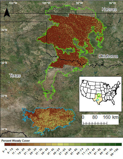
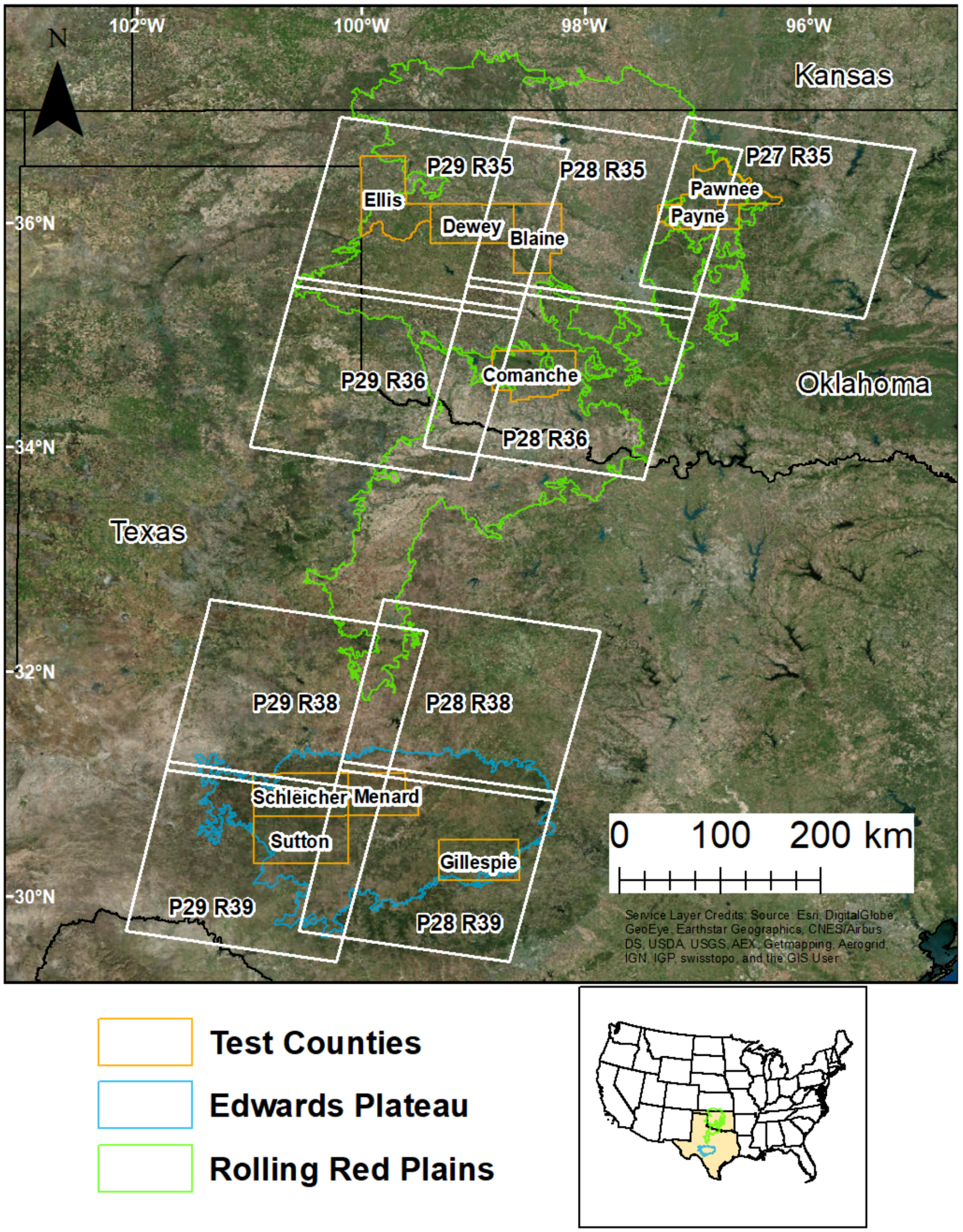
The focus areas of this study are two ecoregions within the Southern Great Plains: Edwards Plateau, located in central Texas, and the Rolling Red Plains located mainly in western Oklahoma and north central Texas. Nine Landsat tiles cover the area of interest (Figure 1).
Edwards Plateau covers around 33,500 km2 with elevation ranging from 240 m to 1200 m. Precipitation, closely related to elevation, varies between 375 and 875 mm per year. The soils are shallow and mainly composed of surface clay turning into rocky clay or solid limestone rock further below the surface. The Plateau contains a variety of short, medium, and tall grasses. Edwards Plateau used to have more fires resulting in a savannah with live oak (Quercus fusiformis) as its primary woody species [38]. Reduced fire frequency and intensity have resulted in more woody cover represented by live oak (Quercus fusiformis), honey mesquite (Prosopis glandulosa), and dense stands of Ashe juniper (Juniperus ashei).
The majority of the Edwards Plateau study area is contained within four Landsat tiles. Path 29 along Rows 38 and 39 covers the western part of the Plateau. Path 28 along Rows 38 and 39 captures the eastern part of the Plateau.
The Rolling Red Plains cover around 269,359 km2 with elevation ranging from 274 m to around 853 m. Mean precipitation varies between 500 and 890 mm annually. The majority of the region is composed of Reddish Prairie and Reddish Chestnut soils [39]. Specific parts of the Plains are composed of Lithosols, Regosols, and Alluvial soils. In the past, the southern portion of the Plains was dominated by a mixture of bluestem (Schizachyrium) and needlegrass (Stipa), while the northern portion was dominated by a combination of oak (Quercus) and bluestem (Schizachyrium) [39]. Now, the region’s woody cover is mainly composed of fragmented stands of Ash Juniper and Eastern Redcedar (Juniperus virginiana L.) [5], with an understory of various grasses, prickly pear (Consolea Lem.), and thorny scrub.
A portion of the Rolling Red Plains ecoregion is contained within five Landsat tiles. The region is composed of three parts: western, central, and eastern. Path 29 along Rows 35 and 36 covers the western part of the Plains. Path 28 along Rows 35 and 36 captures the central part of the Plains. Only one tile, Path 27 Row 35, covers the eastern part of the Plains.
2.2. Overview of Data and Modeling Approach
We explored several approaches to derive woody cover for these ecoregions, including linear spectral mixture models, multivariate regression, and vegetation indices. This manuscript only reports the best approach (Figure 2) and results that follow. Some lessons learned about other approaches are included in the discussion section.
2.3. NAIP and LANDSAT Data Acquisition
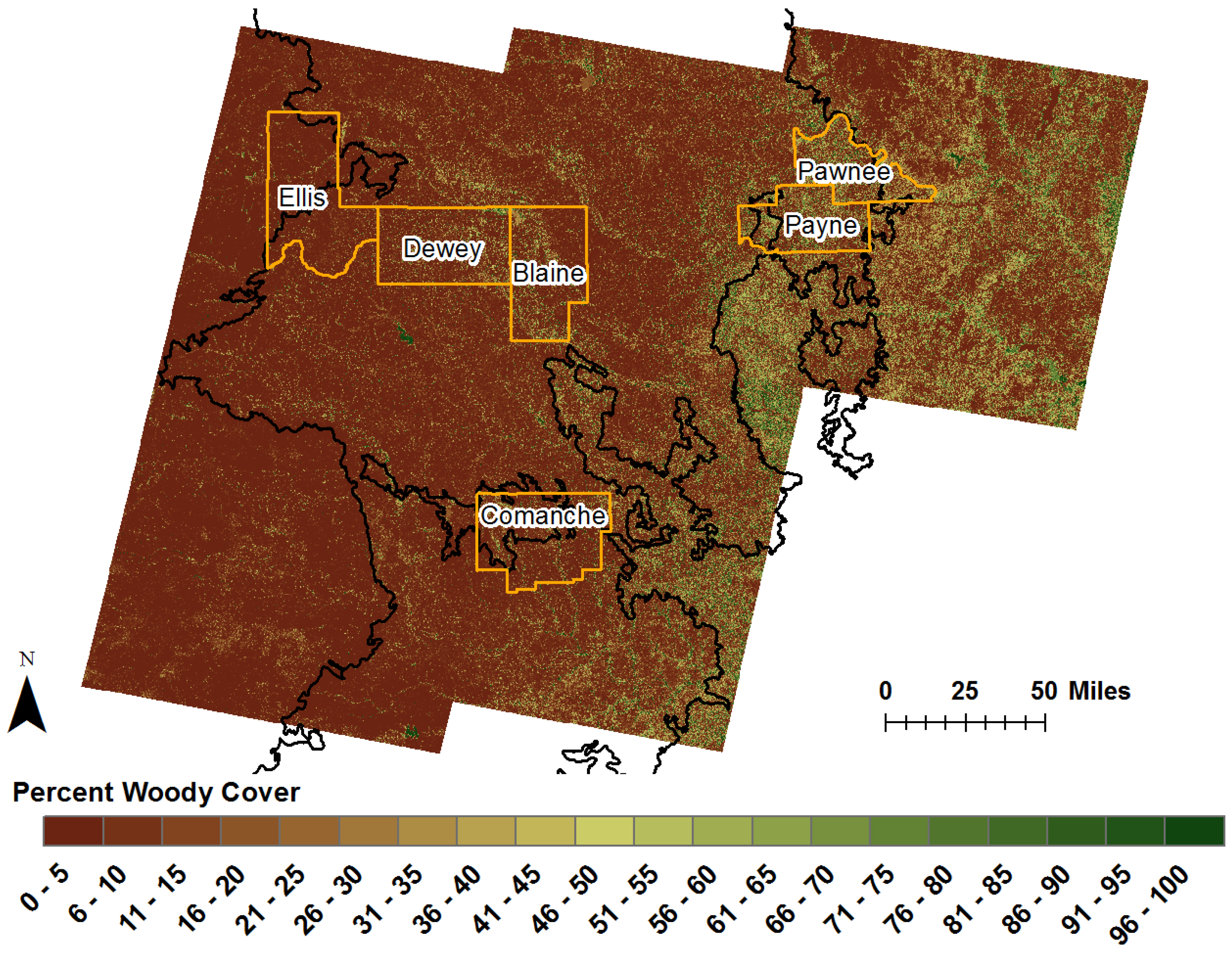
We downloaded National Agriculture Imagery Program (NAIP) county mosaics from the Geospatial Data Gateway (https://gdg.sc.egov.usda.gov/). We selected ten counties in total, with at least two counties located in each of the five portions of the study areas. The 2004 Color infrared mosaics (blue, green, red, NIR) for Edwards Plateau have a spatial resolution of 1 m. Two counties, Schleicher and Sutton, are located in the western portion of Edwards Plateau. The other two counties, Menard and Gillespie, are located in the eastern portion of the Plateau. The 2004 natural color mosaics (blue, green, and red) for the Rolling Red Plains have a spatial resolution of 2 m. Two counties, Ellis and Dewey, are located in the western portion of the Rolling Red Plains. Two counties, Blaine and Comanche, are located in the central portion of the Plains, while the final two counties, Payne and Pawnee, are located in the eastern portion of the ecoregion (Table 1).
We downloaded a selection of Orthorectified and atmospherically corrected 30 m Landsat 5 image data using the USGS EarthExplorer (http://earthexplorer.usgs.gov/) and Land Satellites Data System (LSDS) Science Research and Development (LSRD) Bulk Ordering tool (http://espa.cr.usgs.gov/). The acquired products include Surface reflectance, Normalized Difference Vegetation Index (NDVI), Enhanced Vegetation Index (EVI), Soil Adjusted Vegetation Index (SAVI), Modified Soil Adjusted Vegetation Index (MSAVI), and Normalized Difference Moisture Index (NDMI) for three dates during the year under investigation. Tiles in the same path and acquired on the same day were stitched together using the Mosaic to New Raster tool in ArcGIS (ESRI; Redlands, CA, USA).
To capture the phenological cycle of woody cover and better quantify the amount of woody cover, the selected Landsat data represent the beginning of the growing season, the peak of the growing season, and the end of the growing season (Table 2).
We used image data from 2004 for two reasons. First, cloud-free Landsat data is available for both ecoregions at the key points of the phenological cycle. Secondly, NAIP data is present for both ecoregions. The NAIP datasets have different spatial and spectral resolutions, adding another level of analysis about estimation accuracy addressed later in the paper. We compared products created for 2004 to the closest VCF (2005) and WELD (2006–2010) estimates available. Additionally, we also created Cubist-based woody cover products for 2005 and 2006 to compare coincident years of VCF and WELD products (Appendix A).
We acquired the National Agricultural Statistics Service (NASS) National 2014 Cultivated Layer (https://www.nass.usda.gov/Research_and_Science/Cropland/Release/index.php). The National Cultivated Layer contains information from 2010 to 2014. NASS considered active cropland any pixels classified as cultivated in 2014 or as cultivated in two out of the five years. We masked areas of cropland using the cultivated layer to avoid accidentally classifying the locations as woody cover.
For consistency, between study areas, we used the 2014 Cultivated Layer. The oldest crop data layers available for the two study areas were produced in 2006 (Oklahoma) and 2008 (Texas). Comparison of the 2006 and 2008 crop masks with the 2014 Cultivated Layer revealed that less than 2% of the area in each county reverted from cultivated to non-cultivated. Some of the reversion may be due to the 2006 and 2008 masks being coarser (56 m resolution) than the 2014 layer (30 m). The 2014 Cultivated Layer provided a stable view of the region as it contained five years of data compared to the snapshots documented by the yearly crop data layers.
2.4. Thematic Classification of High Resolution Data
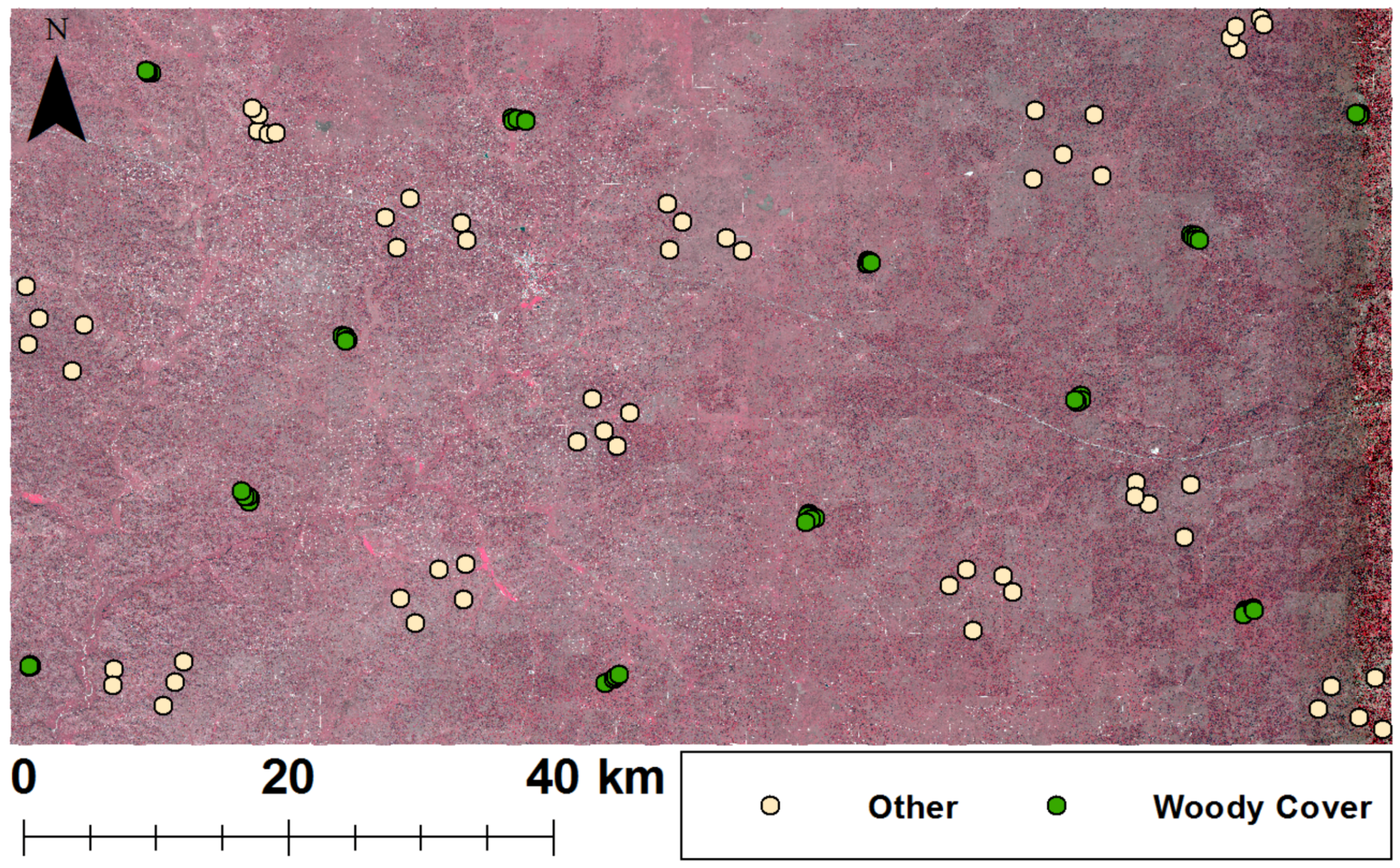
Using ArcMap to perform visual interpretation, we selected 60 NAIP pixels representing woody cover and 60 NAIP pixels representing other cover (Figure 3). We made sure to select woody cover pixels from different canopies within a cluster of canopies. We used a stratified cluster sampling strategy to randomly select pixels from each class and cluster in order to capture signal variation throughout the image and for efficiency (A in Figure 2). Depending on the acquisition date of the fine resolution image data, we also selected pixels representing shadows (other class), grass (other class), or senesced trees (woody cover class) if those classes were present in the NAIP image. We used the Multi-Resolution Land Characteristics Consortium (MRLC) National Land Cover Dataset (NLCD) Mapping Sampling Tool, located in ERDAS Imagine, to select 30 random training pixels from each class, while reserving the remaining 30 pixels from each class for assessment. We then sampled information from every band of the NAIP images also using the MRLC tool.
SEE5, Classification and Regression Tree (CART) software (https://www.rulequest.com/see5-info.html), ingested the sampled information to determine what data to use to separate each class. SEE5 mines through a dataset to find patterns, creates the branches of the CART, and produces a thematic output (B in Figure 2). The algorithm winnows layers deemed insignificant. Boosting was performed with a maximum of ten iterations to achieve the most accurate and unbiased CART result. The software used the 30 random pixels reserved from each class to assess the accuracy of each CART. Error matrices were created to calculate the overall user accuracy, overall kappa, producer’s accuracy for each class, user’s accuracy for each class, and kappa coefficients for each class [40]. The final output is a separate binary land cover raster product for each county in the study (Figure 4).
2.5. Reclass and Aggregation of High Resolution Woody Classification
We merged pixels classified as other, grass, or shadow into one class and combined the pixels representing senesced trees with the woody cover class. The goal was to produce a binary classification containing only woody cover, represented as ones, and other cover, represented as zeroes.
We aggregated the NAIP pixels (1–2 m resolution), classified as woody cover, to calculate the percentage of woody cover present in a Landsat pixel (30 m resolution). The aggregated woody cover was then masked using the NASS cultivated layer to remove any pixels representing cropland (C in Figure 2). We used pixels from these rasters to train the Cubist algorithm, to assess the Cubist algorithm, and to compare the Cubist, WELD, and VCF products.
2.6. Cubist Training and Validation
In a similar vein to SEE5, Cubist is a tool that creates rule-based trees with the output being continuous data (e.g., percent woody cover) instead of thematic values (e.g., woody or not woody) (https://www.rulequest.com/cubist-info.html). Cubist, in this case using the sampled Landsat data, creates various sets of conditions. Depending on what conditions a pixel meets, the software applies a specific linear equation to that pixel to estimate woody cover in that location. Cubist has a number of adjustable settings to fine tune the final modeled output, including a composite option that averages the value of a case based on similar cases and the option to produce an unbiased ruleset.
The stratified sampling strategy option of the MRLC NLCD Mapping Sampling Tool selected 700,000 geographically random pixels, a little more than 1% of the pixels in an average Landsat tile, from each county separately, to train the Cubist algorithm. We set the tool to select pixels, from the aggregated woody cover raster created in Section 2.5, representing woody cover from 1–100%, at 1% increments. The tool used the pixels to sample information from the three Landsat datasets, which included 18 bands of surface reflectance data and 15 indices for each portion of the study area.
Using an iterative process, we ran Cubist a number of times with the same input data and settings, but a different number of training pixels to test if the accuracy changed. The results indicated that the accuracy of the Cubist estimates did not improve much beyond 700,000 training pixels. The software reserved the remaining pixels in each county for validation.
The Cubist software ingested the Landsat information extracted by the training pixels. We selected the “Let Cubist Decide” option and allowed the algorithm to extrapolate 1% to account for the lack of a 0% percent estimation. We did not train a 0% class due to possible confusion related to the variability of soil signatures across the ecoregions.
Cubist assessed the output model using average absolute error magnitude, relative error magnitude, and a correlation coefficient calculated using the reserved validation pixels. The average absolute error magnitude, measured in percent woody cover, is the absolute value of the difference between the reference measurements and the predicted measurements. The relative error magnitude is the average absolute error magnitude divided by the difference between the reference measurements and the mean of the reference measurements. Good models have a value below one. The Pearson correlation coefficient measures the relationship between the reference measurements and the predicted measurements [41].
We performed Cubist woody cover estimates portion by portion (West, Central, East) for the two major study areas. We stitched the portion estimates together, to encompass fully the two regions, using ArcGIS.
We took the following steps to make sure the comparison of the three woody cover products, Cubist, VCF, and WELD, was stringent and thorough. First, we randomly selected 1,000,000 pixels from each county’s aggregated thematic NAIP classification to capture the full range of woody cover. Second, we compared the three products using randomly selected pixels not used for training or assessing the Cubist models compared, as we selected the pixels from another county in the same portion of an ecoregion. This allowed us to determine how well the Cubist estimates performed outside of the county used for sampling, along with how well the estimates compared to the currently available woody cover products. We calculated average absolute errors and correlation values to compare the three products.
We also calculated average errors for each woody cover product at 20 percent intervals 20%, 21–40%, 60%, 80%, and 100%, to examine if certain models over- or under-estimated different levels of woody cover.
3. Results
3.1. SEE5 Classification of NAIP Data
We performed thematic CART classifications for four counties in Texas and six counties in Oklahoma. The majority of the CART models winnowed all but the red wavelength information to distinguish woody cover from other cover. The difference in spatial resolution between the datasets, 1 m and 2 m, did not influence the results, as woody cover is identifiable at both scales. All ten of the county classifications achieved an overall accuracy of 95% or better (Table 3). We also visually inspected the classification products to double check the accuracy measurements.
3.2. Within County Cubist Woody Cover Models
We trained and assessed the 2004 woody cover estimations modelled by Cubist with the ten CART classifications (Figure 5 and Figure 6). The weakest 2004 model, created using pixels from Blaine County, achieved an average absolute error of 17.5 percent woody cover. The strongest model, created with pixels from Menard County, achieved an average absolute error of 8.6 percent woody cover. Averaging the statistics of all the models leads to an average absolute error of 12.1, a relative error of 0.53, and a correlation coefficient of 0.78. All models exhibited correlation coefficients of 0.72 or higher. The evaluations performed using the training data, the same data used to create the models, are slightly better than the evaluations performed with the validation pixels (Table 4).
Broken down by 20% intervals, a pattern emerges in the errors (Table 5). The error related to the 1–20% interval indicates an overestimation of woody cover on average. When estimating woody cover between 21–40%, the errors are low overall, but lean towards underestimation. Estimation for the intervals of 41–60%, 61–80%, and 81–100% reveals that the underestimation of woody cover increases as the level of woody cover estimated increases. Over the full range of woody cover, the errors for each county hover around two percent underestimation.
3.3. Comparison of Cubist and Other Woody Cover Products—External Counties
In order to compare the 2004 woody cover estimates to the VCF and WELD products with confidence, we performed models of woody cover for 2005 and 2006 using the 2004 CART classifications to assess the consistency and stability of woody cover in the region across three consecutive years (Appendix A). The majority of Cubist models exhibited smaller absolute errors than the VCF and WELD woody cover products (Table 6). The correlation between the estimated percent woody cover and the actual percent woody cover tended to be strongest for the Cubist modelled data as well. Overall, the VCF product exhibited the highest average absolute error and the weakest correlations.
3.4. Comparison of Cubist and Other Woody Cover Products at 20 Percent Intervals
The WELD and VCF products had the lowest errors within the 1–20% cover interval (Table 7). On average, the WELD products underestimated woody cover of 1–20% by three percent, while the VCF raster product underestimated by six percent. In the 1–20% cover interval, the Cubist products, on average, overestimated cover by 10 percent.
The Cubist models had the lowest errors within the 21–40% cover interval, with an average error of less than 1%. Both the WELD (−18 percent) and VCF (−26 percent) underestimated woody cover by 18 percent or greater on average for the 21–40% interval.
All three models underestimate woody cover within the 41–60% cover interval. On average, the Cubist models underestimated by 10 percent, the WELD product by 31 percent, and the VCF product by 45 percent.
The amount of underestimation only increases for the 61–80% cover interval. The Cubist model still has the lowest error underestimating by 20 percent on average. The WELD (−43 percent) and VCF (−63 percent) products each have average errors more than double that of the Cubist estimates.
The underestimation errors only increase for the WELD and VCF products when modeling woody cover between 81–100%. The average error for the WELD product was −51 percent and the average error for the VCF product was −82 percent. The Cubist models on average underestimated woody cover in the 81–100% interval by 27 percent.
Examining the overall errors, all three models underestimate woody cover to some degree (Table 8). The average error for the Cubist model was −1 percent, −27 percent for the VCF, and −17 percent for the WELD product. The VCF product underestimated woody cover for all ten counties. The WELD product underestimated woody cover for nine out of the ten counties. The Cubist models overestimated woody cover in five of the counties and underestimated woody cover in the other five.
4. Discussion
Based on the results of this woody cover assessment and research, the Cubist model-based approach does an excellent job of estimating woody cover at the ecoregion scale. However, the VCF and WELD results, for the region, are better than the Cubist models for the 1–20% woody cover interval. The VCF underestimates by 6% on average and the WELD underestimates by 3% on average, while the Cubist overestimates by 10% on average. Acquisition of the training data during peak greenness leads to the overestimation in the Cubist model. Based on the rate of woody cover growth, the majority of woody cover encroachment should appear in the 1–20% interval. To accurately measure encroachment in the region, we need to fine-tune the Cubist model for the low cover interval. In the future, we may explore training using only pixels from 1–20% to see if this improves the estimates created by Cubist.
We must point out that we designed our technique to estimate woody cover across an ecoregion. This means that we accounted for trees and shrubs, no matter their height. The VCF and WELD products model tree cover, not woody cover, across the continental United States. This means that the VCF and WELD models may not account for all shrubs due to height. This may explain the high levels of underestimation by the VCF and WELD products for the 61–80% and 81–100% intervals.
The Cubist technique outperformed other approaches to derive woody cover for these ecoregions, including linear spectral mixture models, multivariate regression, and vegetation indices. The other methods listed above fail to capture the variability of woody cover across the landscape. Linear spectral mixture models need a clear vegetation signal to estimate woody cover, but the ecoregions in the study area contain various types of woody cover. Multivariate regression attempts to create a single equation to model the full range of woody cover, while the Cubist technique creates different equations to account for various ranges of cover related to a variety of species. Vegetation indices are a great input for the modelling algorithms, but attempting to threshold the indices across the entire landscape, to capture all the woody cover, is difficult due to variability in soil and woody type. Cubist integrates the best of all these approaches into an algorithm that can handle the variety of woody cover occurring over a large region.
Image data availability for the area of study is a limitation of the methodology described in this paper. Accurately distinguishing woody cover from other cover types requires high resolution data acquisition at the proper time of year. Avoidance of certain periods of acquisition, such as peak vegetation greenness, minimizes confusion between grass and woody cover. Availability of Landsat scenes throughout the year is equally important to accurately measuring percent woody cover. Our methodology requires scenes from the beginning, middle, and end of the year to capture the phenological cycle of woody cover of both deciduous broadleaf and evergreen species (e.g., oak and juniper) in the area of interest. We wanted to perform a more direct comparison of products by running Cubist for 2005, but NAIP data were unavailable. However, we verified that only a small number of fires occurred in the study area between 2004 and 2005, with a majority of them being low severity [42]. In addition, estimates may not be precise enough for certain applications because of the levels of error present.
Another strength of the Cubist technique is the ability to apply it to any year where both high spatial resolution data and Landsat data are available. Without presenting all results in this manuscript, we also modelled woody cover for the period of 1994–1995 and 2014–2015 using the process described in this paper. We trained the 1994–1995 models with black and white/color infrared DOQQs, with a pixel size of 1m, and Landsat 5 data. The 1994–1995 Cubist models achieved, on average, an average absolute error of 14%, a relative error of 0.55, and a correlation coefficient of 0.74. We trained the 2014–2015 models with 1m natural color NAIP data and Landsat 8 data. The 2014–2015 Cubist models achieved, on average, an average absolute error of 11%, a relative error of 0.48, and a correlation coefficient of 0.82.
Ranchers and land managers provided with accurate and timely estimates of woody cover can make informed decisions on where to rotate cattle and remove woody cover. Studies from around the world show declines in the ability for soil to store carbon in areas where woody encroachment levels have increased [4,43]. In the short term, woody encroachment increases carbon sequestration, but in the long term, it inhibits herbaceous plant growth [3]. Not only do woody plants alter the physical landscape, they also change the access to water resources below the surface. The roots of woody plants can access water resources that grasses cannot, making it possible for woody plants to outcompete grasses and exacerbate encroachment [2]. The ability to create year-to-year percent woody cover maps will help managers get ahead of woody cover expansion.
The EPA reports, that in the future, Texas and Oklahoma will most likely see increases in average temperatures and decreases in average precipitation [44,45]. Dry, hot conditions do not directly translate to decreases in woody cover encroachment [1]. However, if the likelihood of drought does increase, it could lead to greater chances for wildfires. Managers can use year-to-year percent woody cover maps to identify areas that need plant removal or controlled burns to avoid catastrophic uncontrolled fires.
In a future paper, we will use estimates of woody cover from two dates, to compute the change in woody cover for each pixel in the two ecoregions. Measuring change comes with an inherent propagation of error. Cubist produces a raster indicating the possible amount of percent woody cover error for each pixel based on the equation used at that location. Our first inclination is to compute an average absolute error in percent woody cover for each pixel using the average absolute error from the two estimations. Other studies have converted continuous data into categories to handle the error propagation problem [46,47,48]. Building on the idea of categories and fuzzy classifications, we may bin the average absolute errors from each date into ordinal ratings (ex., excellent, good, acceptable, poor, bad). Using the ratings, we would report each pixel’s rating from each date when presenting the amount of percent woody cover change. We would then relate the changes in woody cover to variables such as precipitation, temperature, soil characteristics, fire patterns, and management practices.
5. Conclusions
This research demonstrates that it is possible to create temporally relevant estimates of woody cover using high resolution image data and multi-season Landsat. Current woody cover products only cover a limited time span, 2000–2010, and only certain years, 2000, 2005, and 2010. The methodology laid out in this research allows a user to calculate the percentage of woody cover in an area for any year in the Landsat time series. The results also show that the Cubists estimates tend to be better than the VCF and WELD woody cover products for all parts of a Landsat tile. This was consistently true when we compared the uncertainty between Cubist-based woody cover with VCF and WELD-based woody cover for the years 2004, 2005, and 2006 (Appendix A shows Years 2005 and 2006). The producers of the VCF and WELD products know that errors exist in their products as they are trying to map large, variable areas, the world, and the United States, respectively. However, the methods in this research provide a technician with the means of using a single county of NAIP data to better model regional woody cover over two Landsat tiles.
Accurate woody cover models also provide us with the means of examining the impacts of woody plant expansion or loss on the hydrological cycle. Using our estimates in coordination with the Mapping Evapotranspiration with the high Resolution and Internalized Calibration (METRIC) model, we can calculate evapotranspiration and examine the correlation to woody cover. We can also asses how the amount of evapotranspiration changes over a region with the increase or decrease of woody cover.
Going forward, we plan to use woody cover estimates produced with this methodology to examine the rate of woody cover expansion or loss across Edwards Plateau and the Rolling Red Plains and compare these with results recently published by Wang et al. [34]. The ability to model woody cover nearly every 16 days via Landsat allows us to determine the best temporal interval at which to study this phenomenon. We can determine how quickly specific management activities are changing the landscape, measure how swiftly an area recovers from fire, and study how changes in climate are altering the region.
Acknowledgments
NSF’s Division of Environmental Biology under award number 1413900 funded the research. The National Agricultural Imagery Program (NAIP) provided the fine resolution spectral imagery. The Land Processes Distributed Active Archive Center (LP DAAC), located at USGS/EROS, Sioux Falls, SD, distributes the Landsat data. http://lpdaac.usgs.gov. We thank Jeff Gillan for providing feedback on the initial draft of this manuscript.
Author Contributions
Kyle A. Hartfield and Willem J. D. van Leeuwen conceived and designed the experiments, performed the experiments, analyzed the data, and wrote the paper.
Conflicts of Interest
The authors declare no conflicts of interest.
Appendix A
We performed a series of tests to examine the consistency of woody cover estimates in the study area between 2004 and 2006. We trained the Cubist algorithm using the 2004 NAIP CART classifications and Landsat data from 2005 and 2006 (Table A1 and Table A2).

Table A1.
Locations of Landsat tiles within the ecoregions and the three dates acquired for each portion for the 2005 Cubist woody cover estimates.
Table A1.
Locations of Landsat tiles within the ecoregions and the three dates acquired for each portion for the 2005 Cubist woody cover estimates.
| Ecoregion | Portion | Scene 1 | Scene 2 | Scene 3 | Landsat Path and Row |
|---|---|---|---|---|---|
| Rolling Red Plains | Western | 26 December 2004 | 22 July 2005 | 11 November 2005 | P29 R35-36 |
| Rolling Red Plains | Central | 20 January 2005 | 31 July 2005 | 4 November 2005 | P28 R35-36 |
| Rolling Red Plains | Eastern | 13 January 2005 | 21 May 2005 | 13 November 2005 | P27 R35 |
| Edwards Plateau | Western | 26 December 2004 | 24 September 2005 | 15 February 2006 | P29 R38-39 |
| Edwards Plateau | Eastern | 21 February 2005 | 26 April 2005 | 20 November 2005 | P28 R38-39 |
Table A2.
Locations of Landsat tiles within the ecoregions and the three dates acquired for each portion for the 2006 Cubist woody cover estimates.
Table A2.
Locations of Landsat tiles within the ecoregions and the three dates acquired for each portion for the 2006 Cubist woody cover estimates.
| Ecoregion | Portion | Scene 1 | Scene 2 | Scene 3 | Landsat Path and Row |
|---|---|---|---|---|---|
| Rolling Red Plains | Western | 15 February 2006 | 27 September 2006 | 1 January 2007 | P29 R35-36 |
| Rolling Red Plains | Central | 23 January 2006 | 13 April 2006 | 25 December 2006 | P28 R35-36 |
| Rolling Red Plains | Eastern | 1 February 2006 | 9 June 2006 | 8 March 2007 | P27 R35 |
| Edwards Plateau | Western | 15 February 2006 | 27 September 2006 | 1 January 2007 | P29 R38-39 |
| Edwards Plateau | Eastern | 8 February 2006 | 20 September 2006 | 23 November 2006 | P28 R38-39 |
Results indicate that the average absolute error, relative error, and correlation coefficients remain relatively stable between 2004 and 2005. In some counties, the 2005 Cubist estimates produced estimates of woody cover with less error and strong correlations (Table A3).
Table A3.
Summary of Cubist models run using 2005 Landsat data from the different portions of the ecoregions and sampling data from 10 different counties. We used the 700000 training pixels in each county with the remaining pixels in each county reserved for validation to assess the models. Average Absolute Errors given in percent woody cover.
| Training Pixel Evaluation | Validation Pixel Evaluation | ||||||
|---|---|---|---|---|---|---|---|
| County | Average Absolute Error (%) | Relative Error | Correlation Coefficient | Number of Validation Pixels | Average Absolute Error (%) | Relative Error | Correlation Coefficient |
| Ellis | 9.2 | 0.57 | 0.76 | 331374 | 9.4 | 0.58 | 0.74 |
| Dewey | 14.3 | 0.51 | 0.79 | 108931 | 14.6 | 0.52 | 0.78 |
| Blaine | 17.2 | 0.56 | 0.74 | 704991 | 17.5 | 0.58 | 0.73 |
| Comanche | 11.2 | 0.48 | 0.82 | 619027 | 11.5 | 0.49 | 0.81 |
| Payne | 14.2 | 0.52 | 0.79 | 544162 | 14.5 | 0.54 | 0.78 |
| Pawnee | 14.4 | 0.45 | 0.82 | 143013 | 14.7 | 0.46 | 0.81 |
| Schleicher | 9.0 | 0.47 | 0.84 | 285274 | 9.2 | 0.48 | 0.83 |
| Sutton | 8.6 | 0.47 | 0.86 | 386418 | 8.8 | 0.48 | 0.86 |
| Menard | 8.5 | 0.54 | 0.81 | 193590 | 8.6 | 0.55 | 0.80 |
| Gillespie | 9.8 | 0.55 | 0.79 | 253362 | 10.0 | 0.57 | 0.78 |
When we compared the 2004 models to the 2006 models, the results varied from county to county. Some county estimates exhibited lower errors and stronger correlations, while others exhibited higher errors and lower correlations (Table A4). For example, we measured Blaine County’s average error in 2004 at 17.5 percent and in 2006 at 18.9 percent.
Table A4.
Summary of Cubist models run using 2006 Landsat data from the different portions of the ecoregions and sampling data from 10 different counties. We used the 700000 training pixels in each county with the remaining pixels in each county reserved for validation to assess the models. Average Absolute Errors given in percent woody cover.
| Training Pixel Evaluation | Validation Pixel Evaluation | ||||||
|---|---|---|---|---|---|---|---|
| County | Average Absolute Error (%) | Relative Error | Correlation Coefficient | Number of Validation Pixels | Average Absolute Error (%) | Relative Error | Correlation Coefficient |
| Ellis | 9.7 | 0.60 | 0.72 | 331374 | 9.9 | 0.62 | 0.70 |
| Dewey | 15.5 | 0.55 | 0.76 | 1089301 | 15.8 | 0.57 | 0.74 |
| Blaine | 18.5 | 0.61 | 0.70 | 704991 | 18.9 | 0.62 | 0.68 |
| Comanche | 12.2 | 0.52 | 0.78 | 619027 | 12.5 | 0.53 | 0.77 |
| Payne | 14.1 | 0.52 | 0.79 | 544162 | 14.4 | 0.53 | 0.78 |
| Pawnee | 14.6 | 0.45 | 0.82 | 1430123 | 14.9 | 0.46 | 0.81 |
| Schleicher | 9.6 | 0.50 | 0.82 | 2852704 | 9.7 | 0.51 | 0.81 |
| Sutton | 9.1 | 0.49 | 0.84 | 3864198 | 9.3 | 0.50 | 0.84 |
| Menard | 8.5 | 0.54 | 0.81 | 1935970 | 8.6 | 0.55 | 0.80 |
| Gillespie | 10.2 | 0.58 | 0.77 | 2533672 | 10.4 | 0.59 | 0.76 |
We calculated average absolute errors and correlation coefficients for each county using pixels from the other county in the same portion of the ecoregion for 2004, 2005, and 2006 (Table A5). Results indicate little to no difference between the three years.
Table A5.
Comparison of average absolute errors and correlation coefficients, calculated using pixels from one county in a portion of an ecoregion, of 2004 Cubist models created using training data from another county in the same portion of an ecoregion, to 2005 and 2006 Cubist products. Average Absolute Errors provided in percent woody cover.
| Average Absolute Error (% Woody Cover), Correlation Coefficient | |||
|---|---|---|---|
| Evaluation County | Cubist 2004 | Cubist 2005 | Cubist 2006 |
| Ellis | 16%, 0.57 | 16%, 0.59 | 16%, 0.53 |
| Dewey | 20%, 0.68 | 20%, 0.69 | 21%, 0.67 |
| Blaine | 23%, 0.62 | 22%, 0.63 | 24%, 0.60 |
| Comanche | 23%, 0.65 | 20%, 0.65 | 22%, 0.62 |
| Payne | 26%, 0.66 | 22%, 0.69 | 22%, 0.65 |
| Pawnee | 25%, 0.75 | 22%, 0.75 | 24%, 0.74 |
| Schleicher | 13%, 0.67 | 13%, 0.67 | 14%, 0.56 |
| Sutton | 13%, 0.76 | 11%, 0.77 | 13%, 0.73 |
| Menard | 16%, 0.44 | 16%, 0.48 | 17%, 0.53 |
| Gillespie | 22%, 0.53 | 20%, 0.57 | 24%, 0.55 |
References
- Zeeman, B.J.; Lunt, I.D.; Morgan, J.W. Can severe drought reverse woody plant encroachment in a temperate australian woodland? J. Veg. Sci. 2014, 25, 928–936. [Google Scholar] [CrossRef]
- Gibbens, R.P.; Lenz, J.M. Root systems of some chihuahuan desert plants. J. Arid Environ. 2001, 49, 221–263. [Google Scholar] [CrossRef]
- Hudak, A.T.; Wessman, C.A.; Seastedt, T.R. Woody overstorey effects on soil carbon and nitrogen pools in south african savanna. Aust. Ecol. 2003, 28, 173–181. [Google Scholar] [CrossRef]
- Jackson, R.B.; Banner, J.L.; Jobbágy, E.G.; Pockman, W.T.; Wall, D.H. Ecosystem carbon loss with woody plant invasion of grasslands. Nature 2002, 418, 623. [Google Scholar] [CrossRef] [PubMed]
- Bidwell, T.G.; Engle, D.M.; Moseley, M.E.; Masters, R.E. Invasion of Oklahoma Rangelands and Forests by Eastern Redcedar and Ashe Juniper; Oklahoma State University, Cooperative Extension Service: Stillwater, OK, USA, 2000; 14p. [Google Scholar]
- Ratajczak, Z.; Nippert, J.B.; Collins, S.L. Woody encroachment decreases diversity across North American grasslands and savannas. Ecology 2012, 93, 697–703. [Google Scholar] [CrossRef] [PubMed]
- DeSantis, R.D.; Hallgren, S.W.; Lynch, T.B.; Burton, J.A.; Palmer, M.W. Long-term directional changes in upland Quercus forests throughout Oklahoma, USA. J. Veg. Sci. 2010, 21, 606–618. [Google Scholar] [CrossRef]
- Meneguzzo, D.; Liknes, G.C. Status and trends of eastern redcedar (Juniperus virginiana) in the central United States: Analyses and observations based on forest inventory and analysis data. J. For. 2015, 113, 325–334. [Google Scholar] [CrossRef]
- Asner, G.P.; Archer, S.; Hughes, R.F.; Ansley, R.J.; Wessman, C.A. Net changes in regional woody vegetation cover and carbon storage in texas drylands, 1937–1999. Glob. Chang. Biol. 2003, 9, 316–335. [Google Scholar] [CrossRef]
- Huxman, T.E.; Wilcox, B.P.; Breshears, D.D.; Scott, R.L.; Snyder, K.A.; Small, E.E.; Hultine, K.; Pockman, W.T.; Jackson, R.B. Ecohydrological implications of woody plant encroachment. Ecology 2005, 86, 308–319. [Google Scholar] [CrossRef]
- Patrick, O.R.; Leo, B.M. Vegetative response under various grazing management systems in the Edwards Plateau of Texas. J. Range Manag. 1976, 29, 195–198. [Google Scholar]
- Van Auken, O.W. Causes and consequences of woody plant encroachment into western North American grasslands. J. Environ. Manag. 2009, 90, 2931–2942. [Google Scholar] [CrossRef] [PubMed]
- Van Langevelde, F.; Van De Vijver, C.A.D.M.; Kumar, L.; Van De Koppel, J.; De Ridder, N.; Van Andel, J.; Skidmore, A.K.; Hearne, J.W.; Stroosnijder, L.; Bond, W.J.; et al. Effects of fire and herbivory on the stability of savanna ecosystems. Ecology 2003, 84, 337–350. [Google Scholar] [CrossRef]
- Van De Koppel, J.; Rietkerk, M. Herbivore regulation and irreversible vegetation change in semi-arid grazing systems. Oikos 2000, 90, 253–260. [Google Scholar] [CrossRef]
- Scholes, R.J.; Archer, S.R. Tree-grass interactions in savannas. Annu. Rev. Ecol. Syst. 1997, 28, 517–544. [Google Scholar] [CrossRef]
- DeSantis, R.; Hallgren, S.; Stahle, D. Drought and fire suppression lead to rapid forest composition change in a forest-prairie ecotone. For. Ecol. Manag. 2011, 261, 1833–1840. [Google Scholar] [CrossRef]
- Fuhlendorf, S.D.; Archer, S.A.; Smeins, F.; Engle, D.M.; Taylor, C.A. The combined influence of grazing, fire, and herbaceous productivity on tree–grass interactions. In Western North American Juniperus Communities: A Dynamic Vegetation Type; Van Auken, O.W., Ed.; Springer: New York, NY, USA, 2008; pp. 219–238. [Google Scholar]
- Alofs, K.M.; Fowler, N.L. Loss of native herbaceous species due to woody plant encroachment facilitates the establishment of an invasive grass. Ecology 2013, 94, 751–760. [Google Scholar] [CrossRef] [PubMed]
- Allen, C.D.; Breshears, D.D.; McDowell, N.G. On underestimation of global vulnerability to tree mortality and forest die-off from hotter drought in the anthropocene. Ecosphere 2015, 6, 1–55. [Google Scholar] [CrossRef]
- Schwantes, A.M.; Swenson, J.J.; Jackson, R.B. Quantifying drought-induced tree mortality in the open canopy woodlands of central Texas. Remote Sens. Environ. 2016, 181, 54–64. [Google Scholar] [CrossRef]
- Kennedy, R.E.; Townsend, P.A.; Gross, J.E.; Cohen, W.B.; Bolstad, P.; Wang, Y.Q.; Adams, P. Remote sensing change detection tools for natural resource managers: Understanding concepts and tradeoffs in the design of landscape monitoring projects. Remote Sens. Environ. 2009, 113, 1382–1396. [Google Scholar] [CrossRef]
- Avitabile, V.; Baccini, A.; Friedl, M.A.; Schmullius, C. Capabilities and limitations of landsat and land cover data for aboveground woody biomass estimation of Uganda. Remote Sens. Environ. 2012, 117, 366–380. [Google Scholar] [CrossRef]
- Moleele, N.M.; Ringrose, S.; Matheson, W.; Vanderpost, C. More woody plants? The status of bush encroachment in Botswana’s grazing areas. J. Environ. Manag. 2002, 64, 3–11. [Google Scholar] [CrossRef]
- Huang, C.Y.; Asner, G.P.; Martin, R.E.; Barger, N.N.; Neff, J.C. Multiscale analysis of tree cover and aboveground carbon stocks in pinyon–juniper woodlands. Ecol. Appl. 2009, 19, 668–681. [Google Scholar] [CrossRef] [PubMed]
- Kuhnell, C.A.; Goulevitch, B.M.; Danaher, T.J.; Harris, D.P. Mapping Woody Vegetation Cover over the State of Queensland Using Landsat Tm Imagery. In Proceedings of the 9th Australasian Remote Sensing and Photogrammetry Conference, Sydney, Australia, 20–24 July 1998; pp. 20–24. [Google Scholar]
- Wu, W. Derivation of tree canopy cover by multiscale remote sensing approach. Int. Arch. Photogramm. Remote Sens. Spat. Inf. Sci. 2012, XXXVIII-4/W25, 142–149. [Google Scholar] [CrossRef]
- McCloy, K.R.; Hall, K.A. Mapping the density of woody vegetative cover using landsat mss digital data. Int. J. Remote Sens. 1991, 12, 1877–1885. [Google Scholar] [CrossRef]
- Homer, C.G.; Dewitz, J.A.; Yang, L.; Jin, S.; Danielson, P.; Xian, G.; Coulston, J.; Herold, N.D.; Wickham, J.D.; Megown, K. Completion of the 2011 national land cover database for the conterminous United States-representing a decade of land cover change information. Photogramm. Eng. Remote Sens. 2015, 81, 345–354. [Google Scholar]
- Huang, C.; Yang, L.; Wylie, B.; Homer, C. A Strategy for Estimating Tree Canopy Density using Landsat 7 etm+ and High Resolution Images over Large Areas. In Proceedings of the Third International Conference on Geospatial Information in Agriculture and Forestry, Denver, CO, USA, 5–7 November 2001. [Google Scholar]
- Coulston, J.W.; Moisen, G.G.; Wilson, B.T.; Finco, M.V.; Cohen, W.B.; Brewer, C.K. Modeling percent tree canopy cover: A pilot study. Photogramm. Eng. Remote Sens. 2012, 78, 715–727. [Google Scholar] [CrossRef]
- Flesch, A.D.; Hutto, R.L.; van Leeuwen, W.J.D.; Hartfield, K.; Jacobs, S. Spatial, temporal, and density-dependent components of habitat quality for a desert owl. PLoS ONE 2015, 10, e0119986. [Google Scholar]
- Ramsey, R.D.; Wright, D.L.; McGinty, C. Evaluating the use of landsat 30 m enhanced thematic mapper to monitor vegetation cover in shrub-steppe environments. Geocarto Int. 2004, 19, 39–47. [Google Scholar] [CrossRef]
- Wang, J.; Xiao, X.; Qin, Y.; Dong, J.; Geissler, G.; Zhang, G.; Cejda, N.; Alikhani, B.; Doughty, R.B. Mapping the dynamics of eastern redcedar encroachment into grasslands during 1984–2010 through palsar and time series landsat images. Remote Sens. Environ. 2017, 190, 233–246. [Google Scholar] [CrossRef]
- Wang, J.; Xiao, X.; Qin, Y.; Doughty, R.B.; Dong, J.; Zou, Z. Characterizing the encroachment of juniper forests into sub-humid and semi-arid prairies from 1984 to 2010 using palsar and landsat data. Remote Sens. Environ. 2018, 205, 166–179. [Google Scholar] [CrossRef]
- Sexton, J.O.; Song, X.-P.; Feng, M.; Noojipady, P.; Anand, A.; Huang, C.; Kim, D.-H.; Collins, K.M.; Channan, S.; DiMiceli, C.; et al. Global, 30-m resolution continuous fields of tree cover: Landsat-based rescaling of modis vegetation continuous fields with lidar-based estimates of error. Int. J. Digit. Earth 2013, 6, 427–448. [Google Scholar] [CrossRef]
- Hansen, M.C.; Egorov, A.; Roy, D.P.; Potapov, P.; Ju, J.; Turubanova, S.; Kommareddy, I.; Loveland, T.R. Continuous fields of land cover for the conterminous United States using landsat data: First results from the web-enabled landsat data (weld) project. Remote Sens. Lett. 2011, 2, 279–288. [Google Scholar] [CrossRef]
- Herrmann, S.; Wickhorst, A.; Marsh, S. Estimation of tree cover in an agricultural parkland of senegal using rule-based regression tree modeling. Remote Sens. 2013, 5, 4900–4918. [Google Scholar] [CrossRef]
- Fowler, N.L.; Dunlap, D.W. Grassland vegetation of the eastern Edwards Plateau. Am. Midl. Nat. 1986, 115, 146–155. [Google Scholar] [CrossRef]
- Herbel, C.H. Utilization of grass- and shrublands of the Southwestern United States. In Management of Semi-Arid Ecosystems; Walker, B.H., Ed.; Elsevier: Amsterdam, The Netherlands; Oxford, UK; New York, NY, USA, 1979; Volume 7, pp. 1–408. [Google Scholar]
- Congalton, R.G.; Green, K. Assessing the Accuracy of Remotely Sensed Data: Principles and Practices; CRC Press: Boca Raton, FL, USA, 2008; pp. 1–179. [Google Scholar]
- Quinlan, J.R. C4.5 Programs for Machine Learning; Morgan Kaufmann Publishers: San Mateo, CA, USA, 1993. [Google Scholar]
- Eidenshink, J.C.; Schwind, B.; Brewer, K.; Zhu, Z.-L.; Quayle, B.; Howard, S.M. A project for monitoring trends in burn severity. Fire Ecol. 2007, 3, 3–21. [Google Scholar] [CrossRef]
- Yusuf, H.M.; Treydte, A.C.; Sauerborn, J. Managing semi-arid rangelands for carbon storage: Grazing and woody encroachment effects on soil carbon and nitrogen. PLoS ONE 2015, 10, e0109063. [Google Scholar] [CrossRef] [PubMed]
- EPA. What Climate Change Means for Oklahoma; 430-F-16-038; EPA: San Juan, Puerto Rico, August 2016; 2p. Available online: https://19january2017snapshot.epa.gov/sites/production/files/2016-09/documents/climate-change-ok.pdf (accessed on 5 January 2018).
- EPA. What Climate Change Means for Texas; 430-F-16-045; EPA: San Juan, Puerto Rico, August 2016; 2p. Available online: https://www.epa.gov/sites/production/files/2016-09/documents/climate-change-tx.pdf (accessed on 5 January 2018).
- Burnicki, A.C.; Brown, D.G.; Goovaerts, P. Simulating error propagation in land-cover change analysis: The implications of temporal dependence. Comput. Environ. Urban Syst. 2007, 31, 282–302. [Google Scholar] [CrossRef]
- Riemann, R.; Wilson, B.; Lister, A.; Parks, S. An effective assessment protocol for continuous geospatial datasets of forest characteristics using usfs forest inventory and analysis (fia) data. Remote Sens. Environ. 2010, 114, 2337–2352. [Google Scholar] [CrossRef]
- Sexton, J.O.; Noojipady, P.; Anand, A.; Song, X.-P.; McMahon, S.; Huang, C.; Feng, M.; Channan, S.; Townshend, J.R. A model for the propagation of uncertainty from continuous estimates of tree cover to categorical forest cover and change. Remote Sens. Environ. 2015, 156, 418–425. [Google Scholar] [CrossRef]
Figure 1.
Edwards Plateau (blue) and the Rolling Red Plains (green) are the two ecoregions of focus in this study. Demonstration of the proposed methodology uses ten counties (orange) within nine Landsat tiles (white; with Path (P) and Row(R)).
Figure 1.
Edwards Plateau (blue) and the Rolling Red Plains (green) are the two ecoregions of focus in this study. Demonstration of the proposed methodology uses ten counties (orange) within nine Landsat tiles (white; with Path (P) and Row(R)).

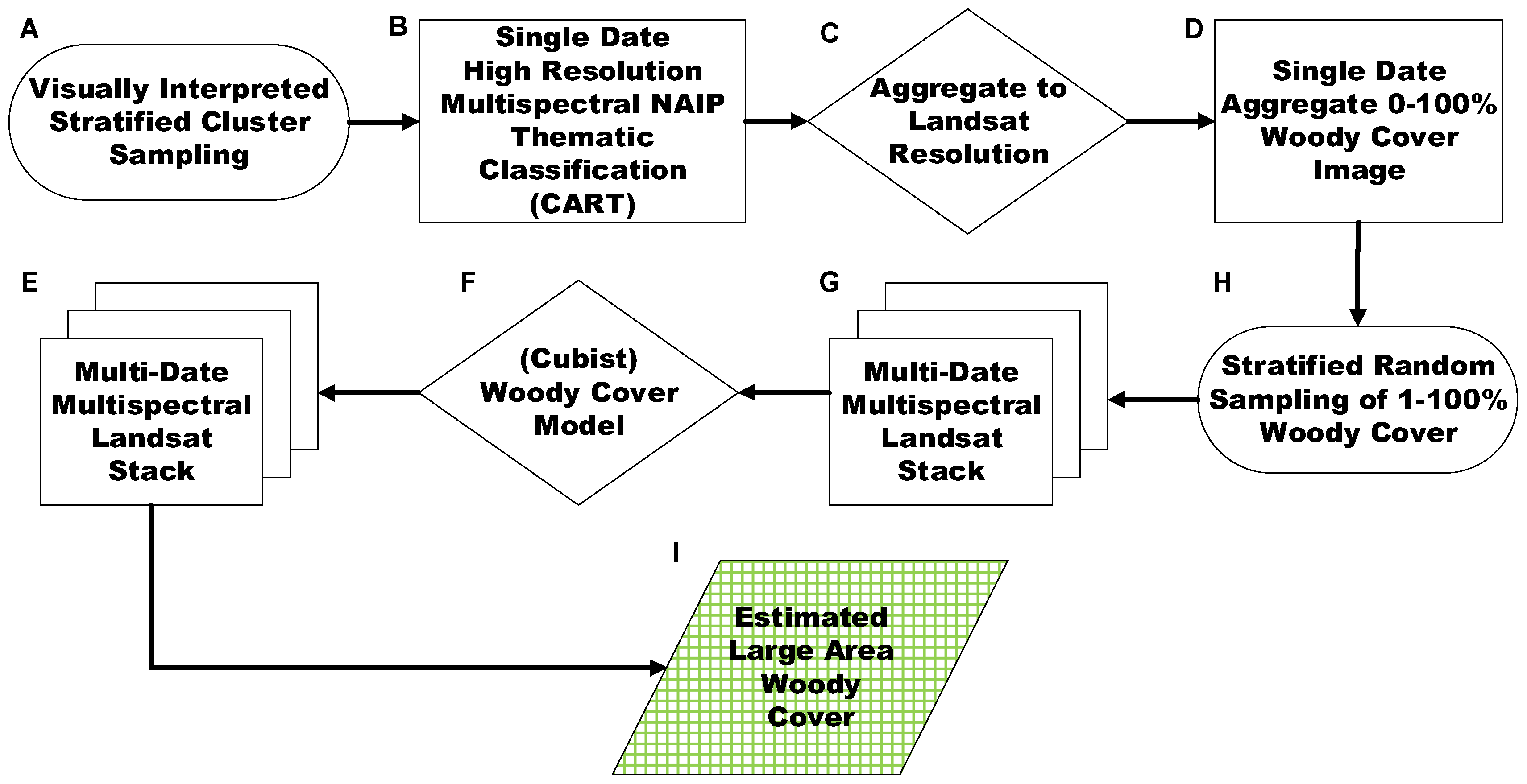
Figure 2.
Flowchart summarizing the processing steps and training of a continuous fractional woody cover model using a CART-based thematic high resolution woody cover classification. Cubist extrapolates the estimated woody over large areas using multi-temporal Landsat data.
Figure 2.
Flowchart summarizing the processing steps and training of a continuous fractional woody cover model using a CART-based thematic high resolution woody cover classification. Cubist extrapolates the estimated woody over large areas using multi-temporal Landsat data.

Figure 3.
Stratified Cluster Sampling Strategy employed to classify 2004 3-band NAIP data for Sutton County, Texas.
Figure 3.
Stratified Cluster Sampling Strategy employed to classify 2004 3-band NAIP data for Sutton County, Texas.

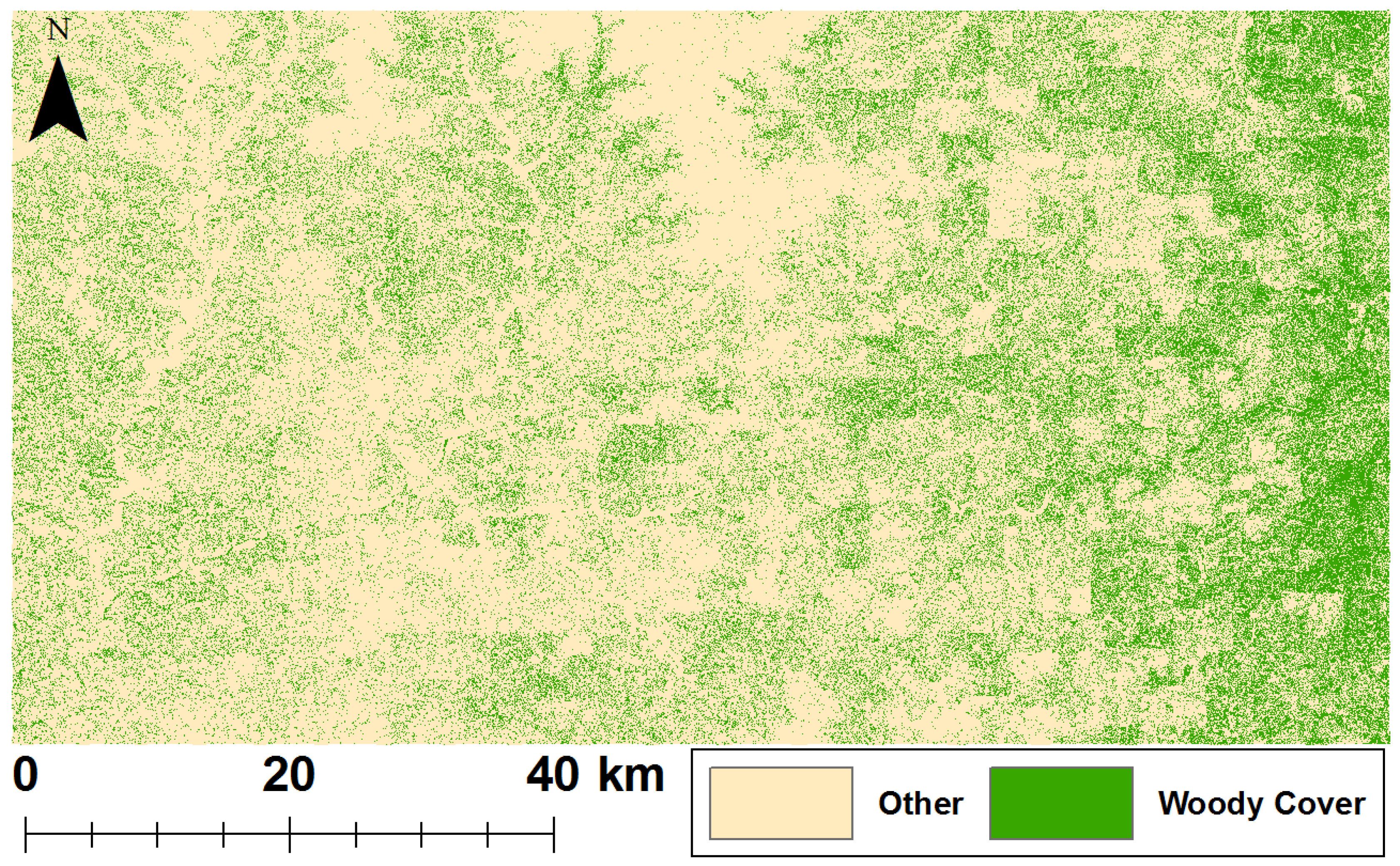
Figure 4.
2004 NAIP binary classification for Sutton County, Texas. Woody cover is green, while all other cover is tan.
Figure 4.
2004 NAIP binary classification for Sutton County, Texas. Woody cover is green, while all other cover is tan.

Figure 5.
Estimated woody cover for 2004 within Edwards Plateau modelled using the Schleicher County- and Menard County-based Cubist models.
Figure 5.
Estimated woody cover for 2004 within Edwards Plateau modelled using the Schleicher County- and Menard County-based Cubist models.

Figure 6.
Estimated woody cover for 2004 within an area of the Rolling Red Plains modelled using the Ellis County-, Comanche County-, and Payne County-based Cubist models.
Figure 6.
Estimated woody cover for 2004 within an area of the Rolling Red Plains modelled using the Ellis County-, Comanche County-, and Payne County-based Cubist models.

Table 1.
Metadata of the NAIP products (2004) for counties in the Rolling Red Plains (RRP) and Edwards Plateau (EP) ecoregions.
Table 1.
Metadata of the NAIP products (2004) for counties in the Rolling Red Plains (RRP) and Edwards Plateau (EP) ecoregions.
| County | Ecoregion | Acquisition Range | Spatial Resolution | Spectral Resolution | Landsat Path and Row |
|---|---|---|---|---|---|
| Ellis | RRP | 3 June–6 June 2004 | 2 m | Natural Color | P29 R35-36 |
| Dewey | RRP | 6 June–13 June 2004 | 2 m | Natural Color | P29 R35-36 |
| Blaine | RRP | 11 June–24 June 2004 | 2 m | Natural Color | P28 R35-36 |
| Comanche | RRP | 1 June–23 June 2004 | 2 m | Natural Color | P28 R35-36 |
| Payne | RRP | 20 July–27 July 2004 | 2 m | Natural Color | P27 R35 |
| Pawnee | RRP | 10 July–2 August 2004 | 2 m | Natural Color | P27 R35 |
| Schleicher | EP | 13 September–26 November 2004 | 1 m | Color Infrared | P29 R38-39 |
| Sutton | EP | 5 November 2004 | 1 m | Color Infrared | P29 R38-39 |
| Menard | EP | 15 July–10 December 2004 | 1 m | Color Infrared | P28 R38-39 |
| Gillespie | EP | 15 July–17 July 2004 | 1 m | Color Infrared | P28 R38-39 |
Table 2.
Locations of Landsat tiles within the ecoregions and the three dates acquired for each portion.
Table 2.
Locations of Landsat tiles within the ecoregions and the three dates acquired for each portion.
| Ecoregion | Portion | Scene 1 | Scene 2 | Scene 3 | Landsat Path and Row |
|---|---|---|---|---|---|
| Rolling Red Plains | Western | 9 January 2004 | 19 July 2004 | 26 December 2004 | P29 R35-36 |
| Rolling Red Plains | Central | 1 December 2003 | 12 July 2004 | 19 December 2004 | P28 R35-36 |
| Rolling Red Plains | Eastern | 31 March 2004 | 7 September 2004 | 12 December 2004 | P27 R35 |
| Edwards Plateau | Western | 26 February 2004 | 1 June 2004 | 26 December 2004 | P29 R38-39 |
| Edwards Plateau | Eastern | 17 December 2003 | 7 April 2004 | 19 December 2004 | P28 R38-39 |
Table 3.
Accuracy assessment results of the CART classifications for each of the counties using 30 pixels representing woody cover and 30 pixels representing non-woody cover.
Table 3.
Accuracy assessment results of the CART classifications for each of the counties using 30 pixels representing woody cover and 30 pixels representing non-woody cover.
| Rolling Red Plains | Overall Accuracy | Edwards Plateau | Overall Accuracy |
|---|---|---|---|
| Ellis | 95% | Schleicher | 100% |
| Dewey | 100% | Sutton | 100% |
| Blaine | 100% | Menard | 98% |
| Comanche | 100% | Gillespie | 100% |
| Payne | 100% | ||
| Pawnee | 98% |
Table 4.
Summary of Cubist models run using 2004 Landsat data from the different portions of the ecoregions and sampling data from 10 different counties. We used the 700,000 training pixels in each county with the remaining pixels in each county reserved for validation to assess the models. Average Errors provided in percent woody cover.
| Training Pixel Evaluation | Validation Pixel Evaluation | ||||||
|---|---|---|---|---|---|---|---|
| County | Average Absolute Error (%) | Relative Error | Correlation Coefficient | Number of Validation Pixels | Average Absolute Error (%) | Relative Error | Correlation Coefficient |
| Ellis | 9.1 | 0.57 | 0.76 | 331374 | 9.3 | 0.58 | 0.74 |
| Dewey | 14.4 | 0.52 | 0.79 | 1089301 | 14.7 | 0.53 | 0.78 |
| Blaine | 17.1 | 0.56 | 0.74 | 704991 | 17.5 | 0.58 | 0.73 |
| Comanche | 11.5 | 0.49 | 0.81 | 619027 | 11.8 | 0.50 | 0.80 |
| Payne | 14.4 | 0.53 | 0.78 | 544162 | 14.6 | 0.54 | 0.78 |
| Pawnee | 14.5 | 0.45 | 0.82 | 1430123 | 14.8 | 0.46 | 0.81 |
| Schleicher | 9.1 | 0.47 | 0.84 | 2852704 | 9.2 | 0.48 | 0.83 |
| Sutton | 9.1 | 0.50 | 0.84 | 3864198 | 9.3 | 0.50 | 0.84 |
| Menard | 8.4 | 0.53 | 0.81 | 1935970 | 8.6 | 0.54 | 0.80 |
| Gillespie | 11 | 0.62 | 0.73 | 2533672 | 11.2 | 0.63 | 0.72 |
Table 5.
Errors calculated by county for different intervals of Cubist woody cover estimation. We calculated the errors in percent woody cover using the reserved validation pixels in each county. The sample size for each 20% interval varies based on the composition of each county. Errors given in percent woody cover.
| Range of Woody Cover Estimated | ||||||
|---|---|---|---|---|---|---|
| Evaluation County | 1–20% | 21–40% | 41–60% | 61–80% | 81–100% | Full |
| Ellis | 2 | −11 | −20 | −26 | −26 | −3 |
| Dewey | 7 | −2 | −9 | −15 | −17 | −2 |
| Blaine | 11 | 1 | −8 | −15 | −20 | −3 |
| Comanche | 4 | −4 | −11 | −17 | −18 | −2 |
| Payne | 8 | 1 | −6 | −13 | −19 | −1 |
| Pawnee | 11 | 2 | −5 | −10 | −10 | −2 |
| Schleicher | 3 | −4 | −11 | −19 | −30 | −2 |
| Sutton | 3 | −3 | −9 | −15 | −18 | −2 |
| Menard | 3 | −5 | −12 | −17 | −22 | −1 |
| Gillespie | 5 | −3 | −10 | −18 | −25 | −1 |
Table 6.
Comparison of average absolute errors and correlation coefficients, calculated using pixels from one county in a portion of an ecoregion, of Cubist models created using training data from another county in the same portion of an ecoregion, to WELD and VCF products. Average Absolute Errors given in percent woody cover.
| Average Absolute Error (% Woody Cover), Correlation Coefficient | |||
|---|---|---|---|
| Evaluation County | Cubist | VCF | WELD |
| Ellis | 16%, 0.57 | 16%, −0.15 | 15%, 0.65 |
| Dewey | 20%, 0.68 | 36%, −0.15 | 26%, 0.51 |
| Blaine | 23%, 0.62 | 43%, 0.22 | 30%, 0.50 |
| Comanche | 23%, 0.65 | 25%, 0.41 | 20%, 0.54 |
| Payne | 26%, 0.66 | 28%, 0.48 | 27%, 0.53 |
| Pawnee | 25%, 0.75 | 42%, 0.56 | 26%, 0.62 |
| Schleicher | 13%, 0.67 | 25%, 0.34 | 26% 0.25 |
| Sutton | 13%, 0.76 | 23%, 0.48 | 26%, 0.34 |
| Menard | 16%, 0.44 | 20%, 0.44 | 22%, 0.30 |
| Gillespie | 22%, 0.53 | 19%, 0.44 | 20%, 0.48 |
Table 7.
Comparison of the average errors present, at 20% increments, in the Cubist (C), WELD (W), and VCF (V) estimates of woody cover across the two ecoregions. We trained the Cubist (C) models with pixels from one county in a portion of an ecoregion and assessed them with a different county in the same portion of the ecoregion. The sample size for each 20% interval varies based on the composition of each county. Errors given in percent woody cover.
| 1–20% | 21–40% | 41–60% | 61–80% | 81–100% | |||||||||||
|---|---|---|---|---|---|---|---|---|---|---|---|---|---|---|---|
| Evaluation County | C | V | W | C | V | W | C | V | W | C | V | W | C | V | W |
| Ellis | 13 | −5 | −3 | 4 | −29 | −21 | −5 | −49 | −36 | −14 | −70 | −50 | −21 | −92 | −61 |
| Dewey | 0 | −7 | −4 | −15 | −30 | −20 | −28 | −50 | −33 | −38 | −70 | −46 | −41 | −93 | −55 |
| Blaine | 3 | −8 | −4 | −10 | −30 | −20 | −2 | −50 | −33 | −32 | −70 | −44 | −39 | −93 | −52 |
| Comanche | 23 | −6 | −1 | 21 | −28 | −12 | 12 | −48 | −23 | 3 | −67 | −33 | −7 | −88 | −37 |
| Payne | 27 | −3 | 13 | 27 | −21 | 10 | 22 | −38 | 3 | 13 | −55 | −6 | −1 | −74 | −17 |
| Pawnee | 0 | −4 | 0 | −16 | −23 | −11 | −28 | −41 | −19 | −38 | −57 | −26 | −38 | −75 | −27 |
| Schleicher | 1 | −6 | −8 | −10 | −28 | −30 | −20 | −47 | −49 | −30 | −65 | −67 | −37 | −82 | −81 |
| Sutton | 11 | −7 | −9 | 6 | −26 | −29 | −1 | −45 | −48 | −9 | −63 | −65 | −14 | −78 | −77 |
| Menard | −1 | −6 | −8 | −19 | −25 | −28 | −35 | −43 | −45 | −49 | −59 | −59 | −59 | −74 | −67 |
| Gillespie | 21 | −3 | −4 | 16 | −20 | −16 | 7 | −36 | −25 | −4 | −52 | −33 | −17 | −68 | −38 |
Table 8.
Comparison of average errors for pixels of 1–100% woody cover, calculated using pixels from one county in a portion of an ecoregion, of Cubist models created using training data from the other county in the same portion of an ecoregion, to WELD and VCF products. Errors given in percent woody cover.
| Average Error for Full (1–100%) Woody Cover Interval | |||
|---|---|---|---|
| Evaluation County | Cubist | VCF | WELD |
| Ellis | 9 | −16 | −11 |
| Dewey | −16 | −36 | −23 |
| Blaine | −16 | −43 | −26 |
| Comanche | 18 | −25 | −11 |
| Payne | 21 | −27 | 5 |
| Pawnee | −23 | −41 | −16 |
| Schleicher | −8 | −24 | −26 |
| Sutton | 6 | −23 | −26 |
| Menard | −13 | −20 | −22 |
| Gillespie | 15 | −17 | −13 |
© 2018 by the authors. Licensee MDPI, Basel, Switzerland. This article is an open access article distributed under the terms and conditions of the Creative Commons Attribution (CC BY) license (http://creativecommons.org/licenses/by/4.0/).
Share and Cite
MDPI and ACS Style
Hartfield, K.A.; Van Leeuwen, W.J.D. Woody Cover Estimates in Oklahoma and Texas Using a Multi-Sensor Calibration and Validation Approach. Remote Sens. 2018, 10, 632. https://doi.org/10.3390/rs10040632
AMA Style
Hartfield KA, Van Leeuwen WJD. Woody Cover Estimates in Oklahoma and Texas Using a Multi-Sensor Calibration and Validation Approach. Remote Sensing. 2018; 10(4):632. https://doi.org/10.3390/rs10040632
Chicago/Turabian StyleHartfield, Kyle A., and Willem J. D. Van Leeuwen. 2018. "Woody Cover Estimates in Oklahoma and Texas Using a Multi-Sensor Calibration and Validation Approach" Remote Sensing 10, no. 4: 632. https://doi.org/10.3390/rs10040632
Note that from the first issue of 2016, this journal uses article numbers instead of page numbers. See further details here.