Groundwater Storage Changes in China from Satellite Gravity: An Overview


1
State Key Laboratory of Geodesy and Earth’s Dynamics, Institute of Geodesy and Geophysics, Chinese Academy of Sciences, Wuhan 430077, China
2
Division of Geodetic Science, School of Earth Sciences, Ohio State University, Columbus, OH 43210, USA
3
State Key Laboratory of Urban Environmental Processes and Digital Modeling, Capital Normal University, Beijing 100048, China
*
Author to whom correspondence should be addressed.
Remote Sens. 2018, 10(5), 674; https://doi.org/10.3390/rs10050674
Submission received: 19 March 2018
/
Revised: 24 April 2018
/
Accepted: 24 April 2018
/
Published: 26 April 2018
(This article belongs to the Special Issue Remote Sensing of Groundwater from River Basin to Global Scales)
Abstract
:Groundwater plays a critical role in the global water cycle and is the drinking source for almost half of the world’s population. However, exact quantification of its storage change remains elusive due primarily to limited ground observations in space and time. The Gravity Recovery and Climate Experiment (GRACE) twin-satellite data have provided global observations of water storage variations at monthly sampling for over a decade and a half, and is enable to estimate changes in groundwater storage (GWS) after removing other water storage components using auxiliary datasets and models. In this paper, we present an overview of GWS changes in three main aquifers within China using GRACE data, and conduct a comprehensive accuracy assessment using in situ ground well observations and hydrological models. GRACE detects a significant GWS depletion rate of 7.2 ± 1.1 km3/yr in the North China Plain (NCP) during 2002–2014, consistent with ground well observations and model predictions. The Liaohe River Basin (LRB) experienced a pronounced GWS decline during 2005–2009, at a depletion rate of 5.0 ± 1.2 km3/yr. Since 2010, GRACE-based GWS reveal a slow recovery in the LRB, with excellent agreement with ground well observations. For the whole study period 2002–2014, no significant long-term GWS depletion is found in the LRB nor in the Tarim Basin. A case study in the Inner Tibetan Plateau highlights there still exist large uncertainties in GRACE-based GWS change estimates.

1. Introduction
Groundwater, as an important component of the global water cycle, is a vital resource of fresh water to sustain agricultural, industrial, and domestic development in many parts of the world, especially in arid and semi-arid regions [1,2]. Globally, groundwater uses in irrigation account for ~43% of the total consumptive irrigation water use [3]. Groundwater also supplies ~50% of drinking water and ~40% of industrial water globally [4]. More than 1.5 billion people worldwide rely on groundwater as the primary source of drinking water [1]. Due to extreme climate episodes, population growth, and extensive groundwater mining and over-exploitation, long-term groundwater depletion has occurred in many regions of the world, exacerbated by various adverse environment impacts, including groundwater quality deterioration, land subsidence, seawater intrusion, and soil salinization [5,6]. Groundwater depletion has been considered as a serious threat to sustainability of water supplies.
From a perspective of water balance, groundwater storage (GWS) change in an aquifer system is referred to as the budget between recharge (e.g., seepage from soil/surface water, and lateral inflow) and discharge (e.g., groundwater withdraws and lateral outflow) [7]. However, it is difficult to quantify groundwater recharge rates and discharge rates directly from in situ hydrological measurements [8]. Alternatively, water level observations from monitoring wells provide the principal source of information on groundwater systems. Groundwater level changes can be further converted to storage changes by multiplying by storage coefficients, e.g., specific yields for unconfined aquifers. However, groundwater levels are often poorly monitored with adequate spatial resolutions due to limited available well networks in many areas around the world.
In addition to being monitored by in situ well observations, GWS changes can be simulated by hydrological models. At global scales, hydrological models can be divided into two categories: land surface models (LSMs) and hydrological water balance models (HMs). Most global LSMs developed by the atmospheric community or climate scientists can simulate water and energy fluxes between the land surface and the atmosphere in general circulation models, which generally can be used to predict soil moisture and water storage changes, but they mostly fail to simulate GWS changes [9,10]. Global HMs, however, are developed for global water resources assessments; therefore, human water uses, e.g., irrigation water use, domestic and industrial water use, are considered in these HMs [10]. Thus, groundwater, as an important source of water use in many arid regions, is generally simulated in the HMs. However, accurate estimation of GWS changes and their trends from global HMs remains a challenge, due to the imperfect parameterization of HMs, the limited knowledge about groundwater recharge/abstractions, and the scarcity of independent ground observations to calibrate models [11]. At regional scales, numerical groundwater flow models can be used to simulate groundwater dynamics and GWS changes in a specific region. To construct a reliable regional groundwater model, however, detailed hydrogeologic data (e.g., hydraulic parameters, water level observations, geology, aquifer materials/channels), climate forcing data, and land use data, among others, need to be collected. It is often difficult to obtain a comprehensive dataset for regional groundwater modeling.
Apart from ground well observations and global/regional models, independent remote sensing-based estimates of water storage changes provide the potential to monitor GWS changes from space. The Gravity Recovery And Climate Experiment (GRACE) twin-satellites provide a direct measure of monthly total water storage (TWS) changes globally at a spatial resolution longer than ~300 km for over a decade and a half since 2002 [12,13]. GRACE-derived TWS changes can be further used to infer GWS changes, if other water storage components from soil moisture, snow/ice, and surface water can be accurately estimated from models or observations and removed from TWS changes [14]. Thus, GRACE represents a powerful tool to estimate GWS changes, especially in regions where groundwater depletion is significant but groundwater levels are unmonitored or poorly monitored. Many studies have successfully used GRACE data to estimate GWS changes especially its depletion in many regions, e.g., in India [15,16,17], California’s Central Valley, USA [18,19], High Plains, USA [20,21] and in the North China Plain (NCP) [22].
As the largest developing country, China has been increasingly experiencing severe water scarcity with rapid population growth and socio-economic development. Especially in the North China, due to drying climate and intensive human activities in the past four decades, groundwater is used and even over-exploited to meet ever-expanding water demand [23,24]. GRACE data have been widely used to estimate TWS/GWS changes over China. Zhong et al. [25] was one of the first to assess long-term TWS changes over the whole China using GRACE. Based on GRACE observations, they found TWS declines in the NCP and the southern Tibetan Plateau (TP) and TWS increase in the Three Gorges Reservoir (TGR) and the Inner TP (ITP) during 2003–2007 [25]. With the increase of GRACE observations over time, seasonal, interannual, and long-term TWS variations in China at basin scales were further analyzed using GRACE [26,27]. Later, numerous case studies have shown that GRACE can be used to detect spatio-temporal TWS/GWS changes and anomalies in many regions of China, which are related to climate extremes and human activities. For example, GRACE successfully detects significant TWS deficits in the Southwestern China during the severe droughts in 2010 and 2011 [28,29]. Similar water storage deficits during droughts are also captured by GRACE in the Yangtze River Basin (YRB) [30,31,32], the Northwest China [33,34], and the North China [35,36]. In addition, considering the water fluxes from a hydrological point of view, GRACE is also used to estimate river discharge in the YRB and human-induced evapotranspiration (ET) change in the NCP [37,38]. By integrating GRACE data into hydrological models, Huang et al. [39] found human-induced TWS increase in the middle and lower reaches of YRB due to intensive irrigation and reservoir operation. Based on GRACE data, some other studies also found human-induced increment in TWS due to water impoundment of TGR in the middle of the Yangtze River [27,40].
In addition to surface water regulation, another potentially significant anthropogenic impact on TWS changes can be groundwater pumping especially in the arid/semiarid North China. Extensive groundwater pumping could lead to irreversible groundwater depletion, which might be detectable for GRACE. In the NCP, Feng et al. [22] found a GWS depletion rate of 8.3 ± 1.1 km3/yr from 2003 to 2010 using GRACE, which can be attributed to intensive groundwater-based irrigation. Since then, several studies reported GRACE-based GWS changes in some regions of China [41,42,43,44,45,46].
According to the World-wide Hydrogeological Mapping and Assessment Programme (WHYMAP), China has three of the world’s thirty-seven large aquifer systems [47], i.e., the North China Aquifer System, the Song-Liao Basin, and the Tarim Basin (Figure 1). The diversity in climate conditions and human activity intensity in these three aquifer systems will result in different GWS changes. Although prior studies have reported GWS changes in some of these aquifers, earlier results did not provide a thorough or comprehensive characterization, nor an elaborate error assessment on the contemporary, i.e., last decade and a half, GWS changes in these aquifers within China. This study provides a quantification of GWS changes in the three main aquifers of China based on comprehensive comparisons of GRACE satellite data, ground well observations, and hydrological models. This paper is organized as follows. In Section 2, we briefly explain the GWS change estimation methods based on GRACE and the data used in this study. Section 3 presents GWS change estimates in three main aquifers of China. In Section 4, we discussed the uncertainties in GRACE-based GWS change estimates, taking the ITP as a case study. The study is summarized and concluded in Section 5.
2. Data and Methodology
2.1. Groundwater Storage Change Estimation from GRACE
GRACE-derived TWS changes represent an integrated change in various water storage components, i.e., soil moisture storage (SMS), snow water equivalent storage (SWES), surface water reservoir storage (RESS), and groundwater storage (GWS). To separate GWS changes from GRACE-derived TWS changes, other water storage components of TWS have to be estimated from auxiliary data or hydrological models. Thus, changes in GWS can be expressed as follows:
Time series of GWS changes in a given region can be estimated by various methods. As we know, original GRACE products in terms of spherical harmonics (SH) (i.e., Stokes coefficients) contain correlated errors in the spectral domain, i.e., north-south stripes in the spatial domain [49]. Thus, destriping (decorrelation) and Gaussian smoothing have to be applied to the GRACE SH products (i.e., Level-2 data) to remove correlated errors and high-frequency noises. The mass variations outside the study region will leak into the region (i.e., leakage-in effect); meanwhile, the signal in the region can also leak out to its surroundings (i.e., leakage-out effect). In general, the composited leakage effect will cause the actual signal inside the region attenuated. In addition, truncation of GRACE SH products with limited degree and order can also result in leakage effect and signal attenuation. Truncation, destriping, and smoothing of SH are hereinafter referred to as filtering or post-processing.
To restore the actual signal in a given region from filtered GRACE products, leakage-in corrections need to be applied, which are estimated by simulated TWS from models generally; and then scaling factor method can be used to restore the leakage-in corrected mass change from filtered GRACE products. There are two methods to estimate scaling factors. In the first method, a basin-scale single scaling factor can be estimated from the ratio of the unfiltered and filtered basin function [50,51,52]. The basin function is defined as 1 inside the basin and 0 outside. The basin-scale scaling factor can also be estimated by minimizing the misfit between unfiltered and filtered mass change time series in the basin from models through least-squares fitting [53]. In the second method, however, gridded scaling factor can be estimated from the ratio of the gridded unfiltered and filtered mass changes from models [53]. No matter which method is used, we can finally derive unbiased time series of TWS changes from GRACE. Then, with estimates on other water storage components from models or observations, we can obtain time series of GWS changes as follows:
where represents scaling factor; subscript represents filtered.
There is another alternative method to derive more reliable GWS changes with a minimum leakage effect if a priori information on GWS changes is available [18]. In this method, other water storage components (SMS, SWES, and RESS) from models are filtered in the same way as the GRACE data. After removing these filtered model grids from GRACE-derived TWS changes, we can obtain filtered GWS grids as follows:
We assume that GWS changes are concentrated inside the area of interest. Therefore, the leakage-in effect should be negligible because there is no GWS change outside the area. Thus, restoring the actual GWS changes only require rescaling of signal amplitude by a scaling factor and no leakage correction is needed:
where represents the scaling factor to restore filtered GWS changes, which needs to be estimated based on independent information on spatial distribution of GWS changes from in situ observations or models. It should be noted that this updated method requires a priori knowledge of GWS changes to obtain the scaling factor.
In addition to traditional SH products, in which leakage reduction and signal restore are needed in the post-processing procedure, GRACE mascon solutions are developed to localize the mass changes at the specific mass concentration (mascon) blocks or mass tiles [54,55]. Correlated errors and signal attenuation can be minimized by applying constraints or regularization during the mascon gravity inversion. A recent comprehensive product intercomparison indicates that mascon solutions are generally consistent with SH products in large-scale basins; however, the variability among different GRACE products, particularly for long-term trends, is also significant especially in small-scale basins, which needs to be evaluated on a case-by-case basis [56,57].
2.2. Data
2.2.1. GRACE Data and Land Surface Models
Monthly GRACE release 5 (RL05) data products, generated by the University of Texas at Austin’s Center for Space Research (CSR), were used to obtain TWS changes. The products were provided in the form of spherical harmonic (SH) coefficients, i.e., Stokes coefficients, up to degree and order 60. The GRACE data were processed as follows. The degree 1 coefficients and the zonal degree 2 coefficients were replaced by more reliable estimates as suggested by Swenson et al. [58] and Cheng et al. [59]. Long-term non-hydrological mass change signal due to the Glacial Isostatic Adjustment (GIA) process was removed based on the model from A et al. [60]. In addition, we applied the DDK4 filter to reduce correlated errors and high-frequency noises in the original SH coefficients [61].
To further estimate GWS changes using GRACE, changes in SMS and SWES were estimated using four versions of LSMs from the Global Land Data Assimilation System (GLDAS), i.e., Noah [62], CLM [63], MOSAIC [64] and VIC [65]. By integrating ground- and space-based observations and using data assimilation techniques, the GLDAS LSMs can simulate optimal fields of land surface water/energy fluxes. The average values of the four versions of LSMs were computed as the final estimates of ΔSMS and ΔSWES. Then, gridded ΔSMS + ΔSWES data are filtered in the same way as the GRACE data and removed from GRACE-derived TWS changes to derive filtered GWS changes, as indicated in Equation (3). Based on the statistics of surface water reservoir storages from the China Water Resources Bulletins (CWRB) published by the Ministry of Water Resources of China (MWR) [66], the ΔRESS trend in the NCP is ~0.3 km3/yr during 2002–2014, which is removed from the GRACE-based GWS rate estimate; while the ΔRESS trends in the other two main aquifers of China are negligible and not considered in the following analysis. To obtain undamped time series of GWS changes from filtered GWS changes based on GRACE and LSMs, we further estimated the scaling factors for recovering actual GWS signals. Gridded GWS changes from the average of two global hydrological models, i.e., the WaterGAP Global Hydrological Model (WGHM), and the PCRaster Global Water Balance (PCR-GLOBWB) model, were used to estimate the scaling factors in the three aquifers of China. These scaling factors were used to derive final time series of GWS changes in our study regions. Considering that Aquifer 1 and 2 (Figure 1) are close to the ocean, the leakage effects due to ocean mass changes might be significant in these two aquifers. We calculated the ocean leakage effects based on the ocean bottom pressure data from the Estimating the Circulation and Climate of the Ocean (ECCO) model and found that the leakage effects on the GWS changes and on the GWS rates are negligible. Thus, leakage is not considered for these aquifers in the following analysis. The uncertainties in GRACE-derived time series of GWS changes were estimated considering the GRACE measurement errors and uncertainties in LSMs. More details on uncertainty estimation can be found in [22].
2.2.2. Hydrological Water Balance Models
The WGHM model and the PCR-GLOBWB model were also used to quantify the spatio-temporal GWS changes in our study regions. The WGHM model simulates water fluxes and storages globally with a spatial resolution of 0.5° × 0.5° [67]. The WGHM model was developed to assess water availability and water uses of the globe, as well as to generate scenarios of changes in water resources. It is worth noticing that, different from most LSMs, the WGHM model considers sectoral water uses for irrigation, livestock, households, manufacturing, and cooling of thermal power plants [68]. Groundwater withdrawals and recharge are simulated in WGHM; thus, we can estimate GWS changes based on these data. In this study, the WGHM model developed by the University of Frankfurt with the version of 2.2b was used [68].
In addition to the WGHM model, we used GWS outputs from the PCR-GLOBWB model, which is also a state-of-the-art grid-based global hydrology and water resources model and developed by the Utrecht University [69,70]. PCR-GLOBWB simulates spatio-temporal water fluxes, e.g., evaporation, discharge, groundwater recharge, and human water use. GWS changes simulated by PCR-GLOBWB have been widely used to quantify the global groundwater depletion rate and its contribution to sea level change [71,72,73]. Both models are forced by the same climate forcing data, i.e., the WATCH Forcing Data methodology applied to ERA-Interim reanalysis data (WFDEI). Monthly gridded GWS changes over China from WGHM and PCR-GLOBWB at 0.5° resolution were used and compared with other estimates in this study.
2.2.3. Ground Well Observations
Groundwater level observations were further collected and analyzed to validate GWS change estimates from GRACE and HMs. For the NCP, monthly water levels from 64 phreatic monitoring wells and 66 confined monitoring wells were obtained from the groundwater yearbooks published by the China Institute of Geological Environment Monitoring (CIGEM) over the period 2005–2013 [74]. Another observation network in the NCP deployed by the MWR contains more than 1000 monitoring wells. However, the original level observations from the network were inaccessible. Fortunately, basin-scale mean level changes over the NCP based on the network were available and used to estimate the temporal variability of GWS changes in the NCP from 2002 to 2014.
For the Song-Liao Basin, water level observations from 151 wells were collected from the CIGEM and the Hydrological Bureau of Inner Mongolia (HBIM) from 2005–2013. It should be noted that, considering the uneven distribution of wells, water levels were averaged over a 1° × 1° mesh where each cell of the mesh was assigned the mean value of water levels within it [20]. Then, mean water level change over the study region was calculated as the area-weighted average of values in all cells of the mesh within the region. For the Tarim Basin, however, water level observations are limited to 6 wells; and half of them contain significant gaps from 2005–2013. Therefore, we fail to estimate GWS changes over the Tarim Basin based on ground well observations.
To estimate GWS changes from ground well observations, level changes should be multiplied by specific yields. For the NCP, the specific yield map based on pumping tests from Zhang et al. [75] was used, with an average of 0.06 over the NCP. For the Song-Liao Basin, a mean specific yield value of 0.09 was used according to pumping tests by Yu et al. [76].
2.2.4. Precipitation Data and Drought Index
Monthly gridded precipitation products from the China Meteorological Data Sharing Service System (CMDSSS) were used to obtain annual precipitation anomalies in our study regions, which are based on 2472 meteorological stations over China and the thin plate spline interpolation method. Additionally, a monthly dataset of Palmer Drought Severity Index (PDSI) on a 2.5° grid was used to quantify the dry or wet conditions in our study regions [77]. The PDSI data used in this study was downloaded from the University Corporation for Atmospheric Research (UCAR), U.S..
3. Results
Figure 2a shows the large-scale spatial variability of GWS rates from GRACE over China during 2002–2014. Among the three main aquifers in China, the North China Aquifer (NCA) experienced the most significant GWS depletion in its northern part (Figure 2a). Both WGHM and PCR-GLOBWB also highlight remarkable GWS depletion in the northern part of NCA, consistent with GRACE results (Figure 2b,c). It should be noted that, in the NCA, the magnitudes of GWS depletion signals from WGHM and PCR-GLOBWB are larger than that from GRACE (Figure 2). It is evident in Figure 2a, which shows the filtered GRACE-based GWS rates in the spatial domain. GRACE also reveals apparent significant GWS depletion in the eastern Himalaya Mountains and the north of the Tarim Basin (Figure 2a). However, these apparent mass loss signals are caused by glacier mass change rather than groundwater depletion, concluded by some previous studies [78,79,80,81]. Note that glacier mass budget is not simulated in LSMs, so glacier mass change signals in these mountain regions still exist in GRACE-derived GWS changes. Spatio-temporal GWS changes in the three main aquifers of China are further discussed as follows.
3.1. North China Plain
The NCP, also known as the Huang-Huai-Hai Plain, is the largest alluvial plain and the most important agriculture base in China (Figure 1). The NCP covers an area of 320,000 km2 with a population of about 300 million. The narrow definition of the NCP, which is more widely used, refer to the plain area between the Taihang Mountains in the northwest and the Yellow River in the southeast, with an area of 140,000 km2 (Figure 3a). Hereinafter, we will adopt this narrow definition of the NCP. From a hydrogeological perspective, the NCP can be divided into three distinct hydrogeological zones: i.e., the piedmont region of the Taihang Mountains, central plain, and coastal plain [82,83], which include all the plains in Beijing and Tianjin municipalities, Hebei province, and northern parts of plains in Henan province and Shandong province. Due to long-term warm and dry climate and intensive anthropogenic activities (agriculture, industry, and urbanization), the groundwater in the NCP has been over-exploited since the 1970s [24]. More than 70% of groundwater exploitation is used for irrigation in the NCP [84,85]. Based on groundwater well observations, some studies have reported long-term groundwater level declines and GWS depletion in some parts of the NCP [24,83,86].
Zhong et al. [25] found the large-scale mass loss in the NCP using GRACE satellites, with a rate of 2.4 cm/yr from 2003 to 2007. Similar mass loss signal in this region was also revealed by other studies [35,36]. Further, Feng et al. [22] concluded that the majority of the mass loss is mainly caused by groundwater depletion in the NCP and found a GWS depletion rate of 8.3 ± 1.1 km3/yr (2.2 ± 0.3 cm/yr) from 2003 to 2010. Since the GWS depletion rate in shallow aquifers from the government reports is only ~2.5 km3/yr in the same time period, far less than the GRACE estimate, Feng et al. [22] concluded that the difference between the estimates from GRACE and official reports indicate the great contribution of GWS depletion from deep aquifers in the NCP. Further study by Huang et al. [43] revealed the heterogeneous GWS change features in the NCP, i.e., faster depletion in the piedmont region of the NCP.
As shown in Figure 3b,d, GRACE-derived GWS rates show the GWS loss in the NCP with relatively coarse spatial resolution and damped magnitude compared to the results from WGHM and PCR-GLOBWB. At a spatial resolution of 0.5 degrees, GWS rates from WGHM and PCR-GLOBWB further highlight the significant GWS depletion in the NCP, consistent with some regional groundwater models [87,88].
Figure 4a,b show groundwater level rates from 2005 to 2013 based on ground monitoring wells in the NCP from unconfined and confined aquifers, respectively. Significant groundwater declines in shallow unconfined aquifers are located in the piedmont region of the Taihang Mountains (Figure 4a); while the groundwater depletion in confined aquifers occurs over the whole plain (Figure 4b).
For shallow unconfined aquifers, GWS changes can be estimated by multiplying phreatic groundwater levels with specific yields. Based on the mean groundwater level changes in the NCP from MWR and the mean specific yield of 0.06, the GWS rate in the NCP is −1.5 km3/yr during 2002–2014. For deep confined aquifers, however, GWS changes contain elastic and inelastic components [89]. Elastic GWS changes can be estimated by multiplying water levels in confined aquifers with elastic storage coefficients. The mean elastic storage coefficient of deep confined aquifers in the NCP is 0.00125, which is about 2% of the mean specific yield of shallow unconfined aquifers [22,87]. Thus, the elastic GWS changes in the NCP is negligible. The other GWS change component, i.e., inelastic GWS changes, represents the irreversible water storage released due to inelastic compaction of the aquifer system [89]. Thus, land subsidence volume represents the change in water storage in the aquifer system [89,90]. Based on the GPS observation network in the NCP, the surface vertical deformation in volume is −6.3 km3/yr from 2002 to 2014 [91]. In Figure 5a, the time series of GWS changes in the NCP from in situ observations represent a sum of GWS changes in unconfined aquifers from monitoring wells and the long-term trend in GWS in confined aquifers from GPS observations.
As shown in Figure 5a, GWS changes in the NCP during 2002–2014 from WGHM and PCR-GLOBWB mainly show a linear decline, at a rate of 12.8 ± 0.2 km3/yr and 9.7 ± 0.2 km3/yr, respectively. GWS depletion rate in the NCP from GRACE is 7.2 ± 1.1 km3/yr for the same time period, which agrees with the result from in situ observations (i.e., 7.8 km3/yr) better than those from WGHM and PCR-GLOBWB. Good agreement between space- and ground-based observations indicates that global hydrological models prone to overestimate the GWS depletion signal in the NCP. For example, Döll et al. [11] also found that WGHM 2.2a overestimates the GWS depletion rate in the NCP in the 2000s (i.e., ~20 km3/yr) by approximately a factor of 4, compared with the independent estimates from GRACE and from regional groundwater models. Döll et al. [11] attribute this overestimation of GWS depletion rate to the strong underestimation of diffuse groundwater recharge in the NCP from WGHM. The updated WGHM 2.2b model, however, improves the simulation of GWS depletion signal in the NCP significantly, although the overestimation still exists.
In addition to linear negative trend signal, GWS changes from in situ observations show significant seasonal variability and interannual fluctuations. GRACE-derived GWS changes agree well with those from in situ observations at seasonal and interannual timescales. Both of them reach maxima in early February. Interannual fluctuations in GWS in the NCP from GRACE and in situ observations show favorable agreement with annual precipitation anomalies. As shown in Figure 5, GRACE-derived GWS recovery for 2003–2004 and 2012–2013 is consistent with positive precipitation anomalies in these years. In contrast, accelerated GWS declines in 2002, 2006 and 2014 inferred from in situ observations and from GRACE can be attributed to the strong droughts in these years (Figure 5).
The values of PDSI in the NCP are generally negative since 2002, which indicate a long-term drying climate in the past decade (Figure 5b). This continuous drought condition in the NCP agrees well with the long-term GWS depletion signal inferred from GRACE, ground observations, and hydrological models. Temporal variability in PDSI, similar to annual precipitation anomalies, is also consistent with interannual GWS changes from GRACE and ground observations (Figure 5).
3.2. Song-Liao Basin
Song-Liao Basin, located in the northeast of China, includes the plain regions of the Songhua River Basin and the Liaohe River Basin (LRB) (Figure 1). In this study, we focus on the GWS changes in the LRB considering the significant GWS depletion and the availability of ground well observations in this region. The LRB is an important grain-production and heavy-industry base in China, covering an area of 260,000 km2. Due to the rapid development of agriculture, industrialization, and urbanization and consequent severe surface water pollution, groundwater has become a major source of water resources utilization in the LRB [92,93,94]. About 60% of water consumption in the LRB is from groundwater in the past decade [66]. Long-term dry conditions and extensive groundwater mining for agricultural, industrial and domestic consumption result in significant groundwater declines in the LRB in the past two decades [94]. Based on GRACE data, Zhao et al. [95] found a GWS decline rate of 13.5 ± 1.9 mm/yr from 2003 to 2010 and the largest GWS depletion rate of 26 mm/yr for 2005–2009 in Horqin Sandy Land, i.e., the upstream of the Liaohe River including Tongliao City, which is consistent with limited six monitoring well observations they collected from the CIGEM. Zhong et al. [46] found a GWS decline rate of 6.8 ± 3.6 mm/yr during 2005–2011 in the western LRB using GRACE.
In the spatial domain, GRACE detects large-scale GWS depletion over the LRB during 2005–2009 (Figure 6b). WGHM shows significant GWS depletion near Tongliao and Shenyang; while PCR-GLOBWB highlights the mass loss near Tongliao and Chifeng (Figure 6c,d). For temporal variability in GWS, GRACE observes obvious interannual GWS variations during 2002–2014 (Figure 7a). GRACE-derived GWS increased during 2002–2005, followed by a significant GWS decline from 2005 to 2009 at a rate of −5.0 ± 1.2 km3/yr (Table 1), and then groundwater recovered again since 2010. GWS results from well observations also show a similar GWS declining rate in 2005–2009 (−5.1 ± 0.5 km3/yr, Table 1) and a GWS increase in 2010–2013, consistent with GRACE results. PCR-GLOBWB, however, only indicates a long-term GWS declining rate, similar to its estimates in the NCP.
Different from PCR-GLOBWB, changes in GWS from WGHM show similar interannual fluctuations as results from GRACE and well observations, but with significantly smaller magnitude (Figure 7b). Note that different scales were used for y-axes in Figure 7a,b. Based on the Groundwater Bulletins of China Northern Plains (GBCNP) and the Groundwater Bulletins of Song-Liao River Basin (GBSLRB) released by the MWR, annual GWS anomalies in the plain area of LRB are in good agreement with results from WGHM at interannual time scales (Figure 7b). It should be noted that the groundwater bulletins only provide annual GWS changes in the plain of LRB. However, the largest GWS depletion occurs in the mountain regions, i.e., in Chifeng, as shown in Figure 8. Thus, the GWS depletion signal from bulletins is less than that from monitoring wells and GRACE. Compared with GRACE and well observations, both WGHM and PCR-GLOBWB underestimate the amplitude of temporal variability of GWS changes signal in the LRB (Figure 7a,b). Nevertheless, in the spatial domain, GWS declines in Chifeng and Tongliao can still be captured by WGHM and PCR-GLOBWB (Figure 6 and Figure 8).
In addition, interannual variability of GWS from GRACE, well observations, WGHM, and groundwater bulletins agrees well with annual precipitation anomalies and PDSI over the LRB. As shown in Figure 7, during the drought conditions from 2006–2009, the GWS declined significantly. Due to more precipitation in 2010 and 2013, the groundwater recovered correspondingly as shown in results from GRACE and WGHM. PCR-GLOBWB, however, fails to simulate interannual GWS variations in the LRB well.
3.3. Tarim Basin
Based on the WHYMAP delineation of world’s largest aquifer systems, the Tarim Basin aquifer is defined as the plain area of Tarim River Basin (TRB), with an area of 450,000 km2 (Figure 1). In addition to the plain area, the entire TRB also includes the southern foot of the Tien Shan Mountains, eastern foot of the Pamir Mountains, and northern foot of the Kunlun Mountains (Figure 9), where melting glaciers and snowpack are primary contributors to streamflow and groundwater recharge over the TRB [96,97]. As the largest endorheic basin in China, the TRB is also known as the driest region on the Eurasian landmass with the Taklamakan Desert in its center occupying 33% of the TRB’s area. The average annual precipitation in the TRB is about 120 mm [98]; while the average annual potential evapotranspiration reaches 1000 mm [99]. Due to increasing temperature in the TRB since the 1970s [98,99], glacier retreat and enhanced snowmelt in the mountain regions of TRB, especially in the Tien Shan Mountains, lead to significant seasonal changes of glacier-fed runoff in the TRB [96].
Although the TRB is extremely arid, GRACE satellites still provide useful information on TWS changes in the basin [34,100,101]. Based on GRACE data, Yang et al. [101] found an increasing TWS rate of 1.6 ± 0.6 mm/yr (1.7 ± 0.6 km3/yr) over the TRB during 2003–2011. However, Yang et al. [34] and Zhao et al. [100] showed a negative GRACE-derived TWS rate of −1.6 ± 1.1 mm/yr and −1.4 ± 0.5 mm/yr during 2002–2015, respectively. The discrepancy between the results in the first study and the following two studies can be attributed to the different time spans used in these studies, considering the significant interannual variability in TWS from 2002 to 2015 in the TRB [34,100]. It should be noted that only gridded Level-3 GRACE products were used in these studies, without considering the leakage errors in the products. Although gridded scaling factors were used in their studies to correct leakage errors and signal attenuation in estimating TWS changes, there are large uncertainties in these scaling factors [53,102]. Because the scaling factors were calculated based on hydrological models, which generally fail to simulate actual TWS changes accurately especially in arid and semiarid regions [102]. Take the TRB as an example, the glacial meltwater from surrounding mountains has a decisive effect on river runoff and water availability over the basin [96]. However, glacier dynamics cannot be included in most models. It will result in large uncertainties in scaling factor estimates, which are calculated based on these models.
As shown in Figure 9, there is no significant or undetectable GWS rate in the TRB simulated by WGHM or PCR-GLOBWB. However, GRACE detects a significant mass increase in the Kunlun Mountains and mass loss in the Tien Shan Mountains. It is worth noting that only changes in soil moisture and snow were simulated from models and subtracted from GRACE-derived TWS changes to obtain GWS changes. Thus, trend signals from other TWS compartments, e.g., glacier and surface water, might be non-negligible and included in GWS rates from GRACE. For the TBR, the mass loss to the north of TBR shown in Figure 9b is confirmed to be attributed to glacier mass loss in the Tien Shan Mountains [78,79]; while the mass increase to the south of TBR can be explained by lake mass increase in the TP [103]. Thus, the nominal GWS rates in these two regions are caused by changes in other TWS compartments rather than GWS. If the entire TBR is included to obtain GWS changes using GRACE and models, significant non-groundwater mass change signals outside the basin will leak into the basin and result in the biased GWS change estimates in the TBR. To reduce the leakage effect, we only calculated the time series of GWS changes in the plain area of TBR, following the definition of the Tarim Basin aquifer from WHYMAP. For temporal variability in GWS, the magnitudes of GWS changes from WGHM and PCR-GLOBWB are far smaller than that from GRACE (Figure 10). An obvious GWS decline from 2006 to 2009 is detected by GRACE (Figure 10a), consistent with less annual precipitation in the same period (Figure 10b).
Unfortunately, there are few long-term monitoring well observations available over the TRB. Only three monitoring wells are located in Korla at the northeast of TRB, with groundwater level data available from 2007 to 2013. For the other three wells in Kashgar at the west of TRB, there are many gaps in groundwater level data. As shown in Figure 11, the groundwater tables are generally deeper in Korla than those in Kashgar. Steady groundwater level declines are observed in Korla at a rate of ~0.6 m/yr during 2007–2013 (Figure 11). Although there is no information on specific yields in the TRB to translate level changes into storage changes, the negative level rate from ground wells is consistent with the GWS decline from GRACE during the same period. Additionally, the well station #3 in Kashgar shows an obvious recovery of water level in 2010, which is also consistent with GRACE-based GWS results and positive annual precipitation in the same year.
4. Discussion
4.1. Errors in GRACE-Derived TWS Changes
According to Equation (1), GWS changes can be estimated as the difference between GRACE-derived TWS changes and non-groundwater storage changes from models. Therefore, uncertainties in GWS changes can be resulted from errors in GRACE-derived TWS changes or from errors in non-groundwater storage changes.
For traditional GRACE products in the form of SH coefficient parameters, errors in TWS changes include GRACE measurement errors and post-processing errors. GRACE measurement errors arise from errors in the measurements of satellite payloads, and errors from the imperfect removal of oceanic and atmospheric mass redistribution during GRACE processing. The measurement errors can be estimated as the root mean square (RMS) of the residuals after removing seasonal cycles and long-term trend from original TWS time series [104]. This method might overestimate the errors if there are significant interannual signals in original time series. In addition, the RMS over the ocean with the same latitude zone as the study region on land can be used empirically as the measurement errors too [105]. These two methods generally give comparable estimates of measurement errors [105].
Given the limited accuracy of GRACE observations and orbit configuration of GRACE satellites, GRACE products are generally expressed as SH coefficients with a limited degree and order. Low signal-to-noise ratios for high degree and order and correlated errors in SH coefficients result in north-south stripes in the spatial domain. Therefore, further post-processing for GRACE data (i.e., destriping and smoothing) is needed to remove noises and stripes, which will inevitably result in signal leakage and attenuation. To obtain unbiased TWS changes, leakage removal and signal rescaling should be considered, which highly depend on model-simulated TWS in general. Signal distortion during destriping and smoothing, i.e., errors in leakage corrections and rescaling, can be considered as post-processing errors.
For GRACE mascon products in terms of mass concentration parameters, the mass changes are defined as point masses or tiles, in which leakage effect is prone to be minimized. For mascon solutions from the Jet Propulsion Laboratory (JPL), errors in gridded TWS results are provided directly [55]. For CSR mascon solutions, however, no error information is available [54]. Thus, the methods for measurement error estimation for traditional SH products can be used to quantify errors in CSR mascon-derived TWS changes [106,107].
In addition to aforementioned uncertainties, TWS changes based on GRACE products from different agencies using various data-processing strategies are likely to show significant discrepancies in some regions. To demonstrate these discrepancies in the spatial domain, we compared the TWS rates over the TP and its surroundings using different GRACE products and post-processing methods. As shown in Figure 12, the most obvious mass loss signal is located in northern India, due to extensive irrigation with groundwater depleted [15,16]. Additionally, there exist significant mass increase in the ITP, which can be attributed to lake mass increase [103] or groundwater increase [108]. However, obvious differences among various methods are illustrated in Figure 12. TWS rates based on CSR SH products with the DDK4 filtering applied show relatively uniform mass increase at the north of ITP (Figure 12b); while TWS rates based on the same products but with 100-km Gaussian smoothing applied highlight three mass increase domes located at the northeast, northwest, and south of ITP, respectively (Figure 12c). However, TWS rates from CSR mascon products only indicate the significant mass gain at the northeast of ITP (Figure 12d). Results from JPL mascon products show two mass increase domes at the northeast and northwest of ITP, respectively (Figure 12e). Figure 12f further shows TWS rates from JPL mascon with scaling factors applied. Significant spatial differences in TWS rates in Figure 12 indicate the potential uncertainty caused by selecting difference GRACE solutions and methods.
4.2. Errors in Non-Groundwater Storage Changes
To obtain GWS changes, other water storage components, simulated by models or measured by observations, need to be removed from GRACE-derived TWS changes. Errors in these components will inevitably result in uncertainties in final GWS estimates. In situ soil moisture monitoring networks are still scarce in most regions of the world. Snow water equivalent products from passive microwave sensors also have large uncertainties [109]. Therefore, simulated SMS and SWES from models are generally used to isolate GWS changes from GRACE-derived TWS changes. However, there are inevitable errors in model-simulated water storage, due to uncertainties in input meteorological forcing data and imperfect simulation of models to mimic actual hydrological processes. RESS from lakes, reservoirs, and rivers can be simulated by some hydrological models or monitored by limited ground- and space-based observations [11,18,19,110].
We take SMS changes in the TP from GLDAS LSMs as an example to demonstrate the uncertainties in models. Figure 13 shows the comparisons of long-term SMS rates from four versions of GLDAS. Although these four GLDAS LSMs adopt the same forcing data, there are still significant discrepancies among these model outputs. The magnitudes of SMS rates from MOSAIC are largest among four models; while the estimates from CLM are far less than those from other three models (Figure 13). The significant differences among them in the TP exemplify the uncertainties in GLDAS LSMs due to different parameterization schemes of land surface. Other reasons for large uncertainty in simulated SM over the TP could be the limitation of available ground hydrometeorological observations to constrain models in this region and the complexity of hydrologic processes among surface water, soil water, glaciers, snowpack, groundwater, and permafrost [111]. Especially, the TP contains the largest alpine permafrost area in the world [112]; while permafrost-related hydrologic processes still fail to be simulated in most global models, which will attribute to large uncertainty in models over the TP. Nearly all GRACE-related mass balance studies on the TP highly reply on hydrological models, only with which other components, e.g., surface water [113], glaciers [80,114], and groundwater [108], can be disaggregated from GRACE-observed total mass changes. Therefore, there would be potentially large uncertainties in these studies, due to imperfectly simulated hydrologic processes in models over the TP. It remains a challenge to quantifying GWS changes in the TP accurately. Fortunately, most of regions, where groundwater has been depleted significantly due to agriculture irrigation or other anthropogenic activities, are in arid or semi-arid plains. Therefore, non-groundwater storage changes and their errors from models are relatively small in these regions. Thus, GRACE along with ancillary models can still be used to estimate long-term GWS changes accurately in places where the contributions from other mass change components are relatively small.
5. Conclusions
GRACE satellites have revolutionized our understanding of the Earth’s gravity field changes, and the inferred mass transport and redistribution. From a hydrological perspective, GRACE provides a novel measure of water storage/flux changes from space, and brings new insights into global/regional water cycling and climate change research. As an important component of terrestrial water, groundwater is poorly monitored by ground observations at regional and global scales. By inferring column-integrated water storage changes from time-variable gravity fields observed by twin satellites, GRACE mission provides a new dimension for measuring GWS changes from space.
Among three main aquifer systems in China, GRACE detects significant GWS depletion in the NCP, with a rate of 7.2 ± 1.1 km3/yr over the period 2003–2014, consistent with the estimate from ground well observations. Compared to GRACE and ground observations, two global HMs (WGHM and PCR-GLOBWB) also captured the GWS depletion signal in this region, but with overestimated rates. Long-term groundwater decline in the NCP can be attributed to a decade-long drought period and intensive groundwater-based irrigation in this region. Ground well observations also highlight the heterogeneous contributions of GWS depletion from different aquifers. In the piedmont region of the Taihang Mountains, groundwater depletion mainly occurred in unconfined aquifers; while groundwater from confined aquifers was depleted over the whole NCP. For the LRB, significant interannual fluctuations in GWS were detected by GRACE, consistent with annual precipitation anomalies in the region. GRACE-derived GWS in the LRB declined at a rate of 5.0 ± 1.2 km3/yr from 2005 to 2009, and recovered slowly since 2010, agreeing remarkably with ground well observations. However, GWS decline rates simulated from WGHM and PCR-GLOBWB are underestimated over the period 2005–2009. Ground well observations highlight that the depletion mainly occurred in the western part of LRB. For the Tarim Basin, in the spatial domain, there is no significant GWS depletion signal within the basin based on GRACE. In addition, there exists significant long-term non-groundwater mass loss/gain signal on the north/south of the basin. Limited ground well observations show groundwater level declines on the north of the basin, consistent with slowly declining time series in GWS from GRACE.
GRACE-based GWS change estimation still contains large uncertainties due to the errors in both GRACE-derived TWS changes and non-groundwater storage changes from models. Any uncertainty in model-simulated storage changes, especially in soil moisture, will result in uncertainties in final GWS estimates. Additionally, potential significant contributions from surface water and glaciers, which are not considered in most LSMs, might cause biases in final GWS estimates too. Another challenge is the errors in GRACE-derived TWS changes. At present, the original GRACE Level-2 products are still dominated by correlated errors; thus, post-processing is needed to suppress the noises, which in turn has resulted in signal attenuation. Current spatial resolution of GRACE is limited to ~300 km or longer, due primarily to intrinsic measurement errors in satellite payloads and the orbit configuration of satellites. Coarse resolution of GRACE also limits its applications in groundwater hydrology [115]. GRACE has ended science operations in September 2017, after more than 15 productive years in orbit [116]. Its successor mission, GRACE Follow-On (GFO), is scheduled to be launched in May 2018 to continue GRACE’s climate data record. A new payload, i.e., the laser-ranging interferometer (LRI), will be on the GFO satellites as an experimental instrument, and on the future Next Generation Gravity Mission (NGGM) satellites. New constellation designs along with LRI onboard NGGM satellites will significantly improve the spatial and temporal resolution of TWS changes as compared to GRACE, and provide a great potential to further enhance our understanding of GWS changes at regional scales in the near future [117].
Author Contributions
W.F. conceived the original experiments; C.K.S. and M.Z. helped improve experimental design; W.F. performed the experiments; W.F. and Y.P. collected and analyzed the data; W.F. wrote the manuscript; C.K.S., M.Z. and Y.P. revised the manuscript.
Acknowledgments
The GRACE solutions used in this study are available from JPL (https://grace.jpl.nasa.gov/). Gridded precipitation products were downloaded from CDMSSSS (http://data.cma.cn/data/cdcindex.html). The PDSI data was downloaded from UCAR (http://www.cgd.ucar.edu/cas/catalog/climind/pdsi.html). This work was jointly funded by the National Natural Science Foundation of China (41431070, 41674084 and 41621091) and the Strategic Priority Research Program of the Chinese Academy of Sciences (XDB23030100). The authors thank Bridget R. Scanlon, Hannes Müller Schmied, and Yulong Zhong for their help to provide data and their processing.
Conflicts of Interest
The authors declare no conflict of interest.
References
- Alley, W.M.; Healy, R.W.; LaBaugh, J.W.; Reilly, T.E. Flow and storage in groundwater systems. Science 2002, 296, 1985–1990. [Google Scholar] [CrossRef] [PubMed]
- Taylor, R.G.; Scanlon, B.; Döll, P.; Rodell, M.; van Beek, R.; Wada, Y.; Longuevergne, L.; Leblanc, M.; Famiglietti, J.S.; Edmunds, M.; et al. Ground water and climate change. Nat. Clim. Chang. 2012, 3, 322–329. [Google Scholar] [CrossRef] [Green Version]
- Siebert, S.; Burke, J.; Faures, J.M.; Frenken, K.; Hoogeveen, J.; Doll, P.; Portmann, F.T. Groundwater use for irrigation—A global inventory. Hydrol. Earth Syst. Sci. 2010, 14, 1863–1880. [Google Scholar] [CrossRef] [Green Version]
- Zektser, I.S.; Everett Lorne, G. Groundwater Resources of the World and Their Use; UNESCO IHP-VI Series on Groundwater No. 6; UNESCO: Paris, France, 2004; p. 346. [Google Scholar]
- Shah, T.; Molden, D.; Sakthivadivel, R.; Seckler, D. The Global Groundwater Situation: Overview of Opportunities and Challenges; International Water Management Institute: Colombo, Sri Lanka, 2000. [Google Scholar]
- Scanlon, B.R.; Jolly, I.; Sophocleous, M.; Zhang, L. Global impacts of conversions from natural to agricultural ecosystems on water resources: Quantity versus quality. Water Resour. Res. 2007, 43, W03437. [Google Scholar] [CrossRef]
- Theis, C.V. The source of water derived from wells. Civ. Eng. 1940, 10, 277–280. [Google Scholar]
- Alley, W.M.; Reilly, T.E.; Franke, O.L. Sustainability of Ground-Water Resources; US Department of the Interior, US Geological Survey: Washington, DC, USA, 1999; Volume 1186.
- Rodell, M.; Houser, P.R.; Jambor, U.; Gottschalck, J.; Mitchell, K.; Meng, C.J.; Arsenault, K.; Cosgrove, B.; Radakovich, J.; Bosilovich, M.; et al. The Global Land Data Assimilation System. Bull. Am. Meteorol. Soc. 2004, 85, 381–394. [Google Scholar] [CrossRef]
- Bierkens, M.F. Global hydrology 2015: State, trends, and directions. Water Resour. Res. 2015, 51, 4923–4947. [Google Scholar] [CrossRef]
- Döll, P.; Müller Schmied, H.; Schuh, C.; Portmann, F.T.; Eicker, A. Global-scale assessment of groundwater depletion and related groundwater abstractions: Combining hydrological modeling with information from well observations and GRACE satellites. Water Resour. Res. 2014, 50, 5698–5720. [Google Scholar] [CrossRef]
- Tapley, B.D.; Bettadpur, S.; Ries, J.C.; Thompson, P.F.; Watkins, M.M. GRACE measurements of mass variability in the Earth system. Science 2004, 305, 503–505. [Google Scholar] [CrossRef] [PubMed]
- Wahr, J.; Molenaar, M.; Bryan, F. Time variability of the Earth’s gravity field: Hydrological and oceanic effects and their possible detection using GRACE. J. Geophys. Res. 1998, 103, 30205–30229. [Google Scholar] [CrossRef]
- Yeh, P.J.F.; Swenson, S.; Famiglietti, J.; Rodell, M. Remote sensing of groundwater storage changes in Illinois using the Gravity Recovery and Climate Experiment (GRACE). Water Resour. Res 2006, 42, W12203. [Google Scholar] [CrossRef]
- Rodell, M.; Velicogna, I.; Famiglietti, J.S. Satellite-based estimates of groundwater depletion in India. Nature 2009, 460, 999–1002. [Google Scholar] [CrossRef] [PubMed]
- Tiwari, V.M.; Wahr, J.; Swenson, S. Dwindling groundwater resources in northern India, from satellite gravity observations. Geophys. Res. Lett. 2009, 36, L18401. [Google Scholar] [CrossRef]
- Long, D.; Chen, X.; Scanlon, B.R.; Wada, Y.; Hong, Y.; Singh, V.P.; Chen, Y.; Wang, C.; Han, Z.; Yang, W. Have GRACE satellites overestimated groundwater depletion in the Northwest India Aquifer? Sci. Rep. 2016, 6, 24398. [Google Scholar] [CrossRef] [PubMed] [Green Version]
- Scanlon, B.R.; Longuevergne, L.; Long, D. Ground referencing GRACE satellite estimates of groundwater storage changes in the California Central Valley, USA. Water Resour. Res. 2012, 48, W04520. [Google Scholar] [CrossRef]
- Famiglietti, J.; Lo, M.; Ho, S.; Bethune, J.; Anderson, K.; Syed, T.; Swenson, S.; de Linage, C.; Rodell, M. Satellites measure recent rates of groundwater depletion in California’s Central Valley. Geophys. Res. Lett. 2011, 38, L03403. [Google Scholar] [CrossRef]
- Strassberg, G.; Scanlon, B.R.; Rodell, M. Comparison of seasonal terrestrial water storage variations from GRACE with groundwater-level measurements from the High Plains Aquifer (USA). Geophys. Res. Lett. 2007, 34, L14402. [Google Scholar] [CrossRef]
- Longuevergne, L.; Scanlon, B.R.; Wilson, C.R. GRACE Hydrological estimates for small basins: Evaluating processing approaches on the High Plains Aquifer, USA. Water Resour. Res. 2010, 46, W11517. [Google Scholar] [CrossRef]
- Feng, W.; Zhong, M.; Lemoine, J.M.; Biancale, R.; Hsu, H.T.; Xia, J. Evaluation of groundwater depletion in North China using the Gravity Recovery and Climate Experiment (GRACE) data and ground-based measurements. Water Resour. Res. 2013, 49, 2110–2118. [Google Scholar] [CrossRef]
- Zheng, C.; Liu, J.; Cao, G.; Kendy, E.; Wang, H.; Jia, Y. Can China cope with its water crisis? Perspectives from the North China Plain. Ground Water 2010, 48, 350–354. [Google Scholar] [CrossRef] [PubMed]
- Liu, C.; Yu, J.; Kendy, E. Groundwater exploitation and its impact on the environment in the North China Plain. Water Int. 2001, 26, 265–272. [Google Scholar]
- Zhong, M.; Duan, J.B.; Xu, H.Z.; Peng, P.; Yan, H.M.; Zhu, Y.Z. Trend of China land water storage redistribution at medi- and large-spatial scales in recent five years by satellite gravity observations. Chin. Sci. Bull. 2009, 54, 816–821. [Google Scholar] [CrossRef]
- Mo, X.; Wu, J.J.; Wang, Q.; Zhou, H. Variations in water storage in China over recent decades from GRACE observations and GLDAS. Nat. Hazards Earth Syst. Sci. 2016, 16, 469–482. [Google Scholar] [CrossRef]
- Yi, S.; Wang, Q.; Sun, W. Basin mass dynamic changes in China from GRACE based on a multibasin inversion method. J. Geophys. Res. 2016, 121, 3782–3803. [Google Scholar] [CrossRef]
- Tang, J.; Cheng, H.; Liu, L. Assessing the recent droughts in Southwestern China using satellite gravimetry. Water Resour. Res. 2014, 50, 3030–3038. [Google Scholar] [CrossRef]
- Long, D.; Shen, Y.; Sun, A.; Hong, Y.; Longuevergne, L.; Yang, Y.; Li, B.; Chen, L. Drought and flood monitoring for a large karst plateau in Southwest China using extended GRACE data. Remote Sens. Environ. 2014, 155, 145–160. [Google Scholar] [CrossRef]
- Zhang, D.; Zhang, Q.; Werner, A.D.; Liu, X. GRACE-based hydrological drought evaluation of the Yangtze River Basin, China. J. Hydrometeorol. 2016, 17, 811–828. [Google Scholar] [CrossRef]
- Zhang, Z.; Chao, B.F.; Chen, J.; Wilson, C.R. Terrestrial water storage anomalies of Yangtze River Basin droughts observed by GRACE and connections with ENSO. Glob. Planet. Chang. 2015, 126, 35–45. [Google Scholar] [CrossRef]
- Zhou, H.; Luo, Z.; Tangdamrongsub, N.; Wang, L.; He, L.; Xu, C.; Li, Q. Characterizing drought and flood events over the Yangtze River Basin using the HUST-Grace2016 solution and ancillary data. Remote Sens. 2017, 9, 1100. [Google Scholar] [CrossRef]
- Cao, Y.; Nan, Z.; Cheng, G. GRACE gravity satellite observations of terrestrial water storage changes for drought characterization in the arid land of northwestern China. Remote Sens. 2015, 7, 1021–1047. [Google Scholar] [CrossRef]
- Yang, P.; Xia, J.; Zhan, C.; Qiao, Y.; Wang, Y. Monitoring the spatio-temporal changes of terrestrial water storage using GRACE data in the Tarim River basin between 2002 and 2015. Sci. Total Environ. 2017, 595, 218–228. [Google Scholar] [CrossRef] [PubMed]
- Su, X.; Ping, J.; Ye, Q. Terrestrial water variations in the North China Plain revealed by the GRACE mission. Sci. China Earth Sci. 2011, 54, 1965–1970. [Google Scholar] [CrossRef]
- Moiwo, J.P.; Yang, Y.H.; Li, H.L.; Han, S.M.; Hu, Y.K. Comparison of GRACE with in situ hydrological measurement data shows storage depletion in Hai River basin, Northern China. Water Sa 2009, 35, 663–670. [Google Scholar] [CrossRef]
- Ferreira, G.V.; Gong, Z.; He, X.; Zhang, Y.; Andam-Akorful, A.S. Estimating total discharge in the Yangtze River Basin using satellite-based observations. Remote Sens. 2013, 5, 3415–3430. [Google Scholar] [CrossRef]
- Pan, Y.; Zhang, C.; Gong, H.; Yeh, P.J.F.; Shen, Y.; Guo, Y.; Huang, Z.; Li, X. Detection of human-induced evapotranspiration using GRACE satellite observations in the Haihe River Basin of China. Geophys. Res. Lett. 2017, 44, 190–199. [Google Scholar] [CrossRef]
- Huang, Y.; Salama, M.; Krol, M.S.; Su, Z.; Hoekstra, A.Y.; Zeng, Y.; Zhou, Y. Estimation of human-induced changes in terrestrial water storage through integration of GRACE satellite detection and hydrological modeling: A case study of the Yangtze River basin. Water Resour. Res. 2015, 51, 8494–8516. [Google Scholar] [CrossRef]
- Wang, X.; de Linage, C.; Famiglietti, J.; Zender, C.S. Gravity Recovery and Climate Experiment (GRACE) detection of water storage changes in the Three Gorges Reservoir of China and comparison with in situ measurements. Water Resour. Res. 2011, 47, W12502. [Google Scholar] [CrossRef]
- Jiao, J.J.; Zhang, X.; Wang, X. Satellite-based estimates of groundwater depletion in the Badain Jaran Desert, China. Sci. Rep. 2015, 5, 8960. [Google Scholar] [CrossRef] [PubMed] [Green Version]
- Hu, L.; Jiao, J. Calibration of a large-scale groundwater flow model using GRACE data: A case study in the Qaidam Basin, China. Hydrogeol. J. 2015, 1–13. [Google Scholar] [CrossRef]
- Huang, Z.; Pan, Y.; Gong, H.; Yeh, P.J.F.; Li, X.; Zhou, D.; Zhao, W. Subregional-scale groundwater depletion detected by GRACE for both shallow and deep aquifers in North China Plain. Geophys. Res. Lett. 2015, 42, 1791–1799. [Google Scholar] [CrossRef]
- Moiwo, J.P.; Lu, W.; Tao, F. GRACE, GLDAS and measured groundwater data products show water storage loss in Western Jilin, China. Water Sci. Technol. 2012, 65, 1606–1614. [Google Scholar] [CrossRef] [PubMed]
- Huo, A.; Peng, J.; Chen, X.; Deng, L.; Wang, G.; Cheng, Y. Groundwater storage and depletion trends in the Loess areas of China. Environ. Earth Sci. 2016, 75, 1167. [Google Scholar] [CrossRef]
- Zhong, Y.; Zhong, M.; Feng, W.; Zhang, Z.; Shen, Y.; Wu, D. Groundwater depletion in the West Liaohe River Basin, China and its Implications revealed by GRACE and in situ measurements. Remote Sens. 2018, 10, 493. [Google Scholar] [CrossRef]
- World-wide Hydrogeological Mapping and Assessment Programme. Available online: http://ihp-wins.unesco.org/layers/geonode:world_aquifer_systems (accessed on 15 December 2017).
- Pfeffer, J.; Seyler, F.; Bonnet, M.-P.; Calmant, S.; Frappart, F.; Papa, F.; Paiva, R.C.D.; Satgé, F.; Silva, J.S.D. Low-water maps of the groundwater table in the central Amazon by satellite altimetry. Geophys. Res. Lett. 2014, 41, 1981–1987. [Google Scholar] [CrossRef]
- Swenson, S.; Wahr, J. Post-processing removal of correlated errors in GRACE data. Geophys. Res. Lett. 2006, 33, L08402. [Google Scholar] [CrossRef]
- Velicogna, I.; Wahr, J. Acceleration of Greenland ice mass loss in spring 2004. Nature 2006, 443, 329–331. [Google Scholar] [CrossRef] [PubMed]
- Chen, J.L.; Wilson, C.R.; Famiglietti, J.S.; Rodell, M. Spatial sensitivity of the Gravity Recovery and Climate Experiment (GRACE) time-variable gravity observations. J. Geophys. Res. 2005, 110, B8408. [Google Scholar] [CrossRef]
- Klees, R.; Zapreeva, E.A.; Winsemius, H.C.; Savenije, H.H.G. The bias in GRACE estimates of continental water storage variations. Hydrol. Earth Syst. Sci. 2007, 11, 1227–1241. [Google Scholar] [CrossRef]
- Landerer, F.; Swenson, S. Accuracy of scaled GRACE terrestrial water storage estimates. Water Resour. Res. 2012, 48, W04531. [Google Scholar] [CrossRef]
- Save, H.; Bettadpur, S.; Tapley, B.D. High-resolution CSR GRACE RL05 mascons. J. Geophys. Res. 2016, 121, 7547–7569. [Google Scholar] [CrossRef]
- Watkins, M.M.; Wiese, D.N.; Yuan, D.-N.; Boening, C.; Landerer, F.W. Improved methods for observing Earth’s time variable mass distribution with GRACE using spherical cap mascons. J. Geophys. Res. 2015, 120, 2648–2671. [Google Scholar] [CrossRef]
- Scanlon, B.R.; Zhang, Z.; Save, H.; Wiese, D.N.; Landerer, F.W.; Long, D.; Longuevergne, L.; Chen, J. Global evaluation of new GRACE mascon products for hydrologic applications. Water Resour. Res. 2016, 52, 9412–9429. [Google Scholar] [CrossRef]
- Long, D.; Pan, Y.; Zhou, J.; Chen, Y.; Hou, X.; Hong, Y.; Scanlon, B.R.; Longuevergne, L. Global analysis of spatiotemporal variability in merged total water storage changes using multiple GRACE products and global hydrological models. Remote Sens. Environ. 2017, 192, 198–216. [Google Scholar] [CrossRef]
- Swenson, S.; Chambers, D.; Wahr, J. Estimating geocenter variations from a combination of GRACE and ocean model output. J. Geophys. Res. 2008, 113, B08410. [Google Scholar] [CrossRef]
- Cheng, M.; Tapley, B.D.; Ries, J.C. Deceleration in the Earth’s oblateness. J. Geophys. Res. 2013, 118, 740–747. [Google Scholar] [CrossRef]
- Wahr, J.; Zhong, S. Computations of the viscoelastic response of a 3-D compressible Earth to surface loading: An application to Glacial Isostatic Adjustment in Antarctica and Canada. Geophys. J. Int. 2013, 192, 557–572. [Google Scholar]
- Kusche, J.; Schmidt, R.; Petrovic, S.; Rietbroek, R. Decorrelated GRACE time-variable gravity solutions by GFZ, and their validation using a hydrological model. J. Geod. 2009, 83, 903–913. [Google Scholar] [CrossRef]
- Ek, M.; Mitchell, K.; Lin, Y.; Rogers, E.; Grunmann, P.; Koren, V.; Gayno, G.; Tarpley, J. Implementation of Noah land surface model advances in the National Centers for Environmental Prediction operational mesoscale Eta model. J. Geophys. Res. Atmos. 2003, 108. [Google Scholar] [CrossRef]
- Dai, Y.J.; Zeng, X.B.; Dickinson, R.E.; Baker, I.; Bonan, G.B.; Bosilovich, M.G.; Denning, A.S.; Dirmeyer, P.A.; Houser, P.R.; Niu, G.Y.; et al. The Common Land Model. Bull. Am. Meteorol. Soc. 2003, 84, 1013–1023. [Google Scholar] [CrossRef]
- Koster, R.D.; Suarez, M.J. Modeling the land surface boundary in climate models as a composite of independent vegetation stands. J. Geophys. Res. Atmos. 1992, 97, 2697–2715. [Google Scholar] [CrossRef]
- Liang, X.; Lettenmaier, D.P.; Wood, E.F.; Burges, S.J. A simple hydrologically based model of land surface water and energy fluxes for general circulation models. J. Geophys. Res. Atmos. 1994, 99, 14415–14428. [Google Scholar] [CrossRef]
- Ministry of Water Resources of China (MWR). China Water Resources Bulletin; MWR: Beijing, China, 2015. [Google Scholar]
- Alcamo, J.; Döll, P.; Henrichs, T.; Kaspar, F.; Lehner, B.; Rösch, T.; Siebert, S. Development and testing of the WaterGAP 2 global model of water use and availability. Hydrol. Sci. J. 2003, 48, 317–337. [Google Scholar] [CrossRef]
- Müller Schmied, H.; Eisner, S.; Franz, D.; Wattenbach, M.; Portmann, F.T.; Flörke, M.; Döll, P. Sensitivity of simulated global-scale freshwater fluxes and storages to input data, hydrological model structure, human water use and calibration. Hydrol. Earth Syst. Sci. 2014, 18, 3511–3538. [Google Scholar] [CrossRef]
- Van Beek, L.P.H.; Wada, Y.; Bierkens, M.F.P. Global monthly water stress: 1. Water balance and water availability. Water Resour. Res. 2011, 47, W07517. [Google Scholar] [CrossRef]
- Sutanudjaja, E.H.; van Beek, R.; Wanders, N.; Wada, Y.; Bosmans, J.H.C.; Drost, N.; van der Ent, R.J.; de Graaf, I.E.M.; Hoch, J.M.; de Jong, K.; et al. PCR-GLOBWB 2: A 5 arc-minute global hydrological and water resources model. Geosci. Model Dev. Discuss. 2017, 2017, 1–41. [Google Scholar] [CrossRef]
- Wada, Y.; van Beek, L.P.H.; van Kempen, C.M.; Reckman, J.W.T.M.; Vasak, S.; Bierkens, M.F.P. Global depletion of groundwater resources. Geophys. Res. Lett. 2010, 37, L20402. [Google Scholar] [CrossRef]
- Wada, Y.; van Beek, L.P.H.; Sperna Weiland, F.C.; Chao, B.F.; Wu, Y.-H.; Bierkens, M.F.P. Past and future contribution of global groundwater depletion to sea-level rise. Geophys. Res. Lett. 2012, 39, L09402. [Google Scholar] [CrossRef]
- Konikow, L.F. Contribution of global groundwater depletion since 1900 to sea-level rise. Geophys. Res. Lett. 2011, 38, L17401. [Google Scholar] [CrossRef]
- China Institute of Geological Environment Monitoring (CIGEM). China Geological Environment Monitoring: Groundwater Yearbook; China Land Press: Beijing, China, 2013. [Google Scholar]
- Zhang, Z.J.; Fei, Y.H. Altas of Groundwater Sustainable Utilization in North China Plain; China Cartographic Publishing House: Beijing, China, 2009. [Google Scholar]
- Yu, C. Dynamic Simulation Evaluation about Water Resource System and Optimal Allocation Model of Macro-Economy Water Resource in Tongliao City; Inner Mongolia Agricultural University: Hohhot, China, 2004. [Google Scholar]
- Dai, A.; Trenberth, K.E.; Qian, T. A global dataset of Palmer Drought Severity Index for 1870–2002: Relationship with soil moisture and effects of surface warming. J. Hydrometeorol. 2004, 5, 1117–1130. [Google Scholar] [CrossRef]
- Farinotti, D.; Longuevergne, L.; Moholdt, G.; Duethmann, D.; Molg, T.; Bolch, T.; Vorogushyn, S.; Guntner, A. Substantial glacier mass loss in the Tien Shan over the past 50 years. Nat. Geosci. 2015, 8, 716–722. [Google Scholar] [CrossRef]
- Yi, S.; Wang, Q.; Chang, L.; Sun, W. Changes in mountain glaciers, lake levels, and snow coverage in the Tianshan monitored by GRACE, ICESat, altimetry, and MODIS. Remote Sens. 2016, 8, 798. [Google Scholar] [CrossRef]
- Jacob, T.; Wahr, J.; Pfeffer, W.T.; Swenson, S. Recent contributions of glaciers and ice caps to sea level rise. Nature 2012, 482, 514–518. [Google Scholar] [CrossRef] [PubMed]
- Gardner, A.S.; Moholdt, G.; Cogley, J.G.; Wouters, B.; Arendt, A.A.; Wahr, J.; Berthier, E.; Hock, R.; Pfeffer, W.T.; Kaser, G.; et al. A reconciled estimate of glacier contributions to sea level rise: 2003 to 2009. Science 2013, 340, 852–857. [Google Scholar] [CrossRef] [PubMed] [Green Version]
- Wu, C.; Xu, Q.; Zhang, X.; Ma, Y. Palaeochannels on the North China Plain: Types and distributions. Geomorphology 1996, 18, 5–14. [Google Scholar]
- Foster, S.; Garduno, H.; Evans, R.; Olson, D.; Tian, Y.; Zhang, W.; Han, Z. Quaternary aquifer of the North China Plain--Assessing and achieving groundwater resource sustainability. Hydrogeol. J. 2004, 12, 81–93. [Google Scholar] [CrossRef]
- Liu, J.; Cao, G.; Zheng, C. Sustainability of groundwater resources in the North China Plain. In Sustaining Groundwater Resources; Jones, J.A.A., Ed.; Springer: New York, NY, USA, 2011; pp. 69–87. [Google Scholar]
- Wang, J.; Huang, J.; Blanke, A.; Huang, Q.; Rozelle, S. The development, challenges and management of groundwater in rural China. In Groundwater in Developing World Agriculture: Past, Present and Options for a Sustainable Future; Giordano, M., Shah, T., Eds.; International Water Management Institute: Colombo, Sri Lanka, 2007; pp. 37–62. [Google Scholar]
- Kendy, E.; Zhang, Y.; Liu, C.; Wang, J.; Steenhuis, T. Groundwater recharge from irrigated cropland in the North China Plain: Case study of Luancheng County, Hebei Province, 1949–2000. Hydrol. Process. 2004, 18, 2289–2302. [Google Scholar] [CrossRef]
- Cao, G.; Zheng, C.; Scanlon, B.R.; Liu, J.; Li, W. Use of flow modeling to assess sustainability of groundwater resources in the North China Plain. Water Resour. Res. 2013, 49, 159–175. [Google Scholar] [CrossRef]
- Qin, H.; Cao, G.; Kristensen, M.; Refsgaard, J.C.; Rasmussen, M.O.; He, X.; Liu, J.; Shu, Y.; Zheng, C. Integrated hydrological modeling of the North China Plain and implications for sustainable water management. Hydrol. Earth Syst. Sci. 2013, 17, 3759–3778. [Google Scholar] [CrossRef] [Green Version]
- Faunt, C.C.; Hanson, R.; Belitz, K.; Schmid, W.; Predmore, S.; Rewis, D. Groundwater Availability of the Central Valley Aquifer, California; US Geological Survey: Reston, VI, USA, 2009.
- Guo, H.; Zhang, Z.; Cheng, G.; Li, W.; Li, T.; Jiao, J.J. Groundwater-derived land subsidence in the North China Plain. Environ. Earth Sci. 2015, 74, 1415–1427. [Google Scholar] [CrossRef]
- Liang, S.; Gan, W.; Shen, C.; Xiao, G.; Liu, J.; Chen, W.; Ding, X.; Zhou, D. Three-dimensional velocity field of present-day crustal motion of the Tibetan Plateau derived from GPS measurements. J. Geophys. Res. 2013, 118, 5722–5732. [Google Scholar] [CrossRef]
- Xia, J.; Chen, Y.D. Water problems and opportunities in the hydrological sciences in China. Hydrol. Sci. J. 2001, 46, 907–921. [Google Scholar]
- Zhang, X.; Xu, K.; Zhang, D. Risk assessment of water resources utilization in Songliao Basin of Northeast China. Environ. Earth Sci. 2012, 67, 1319–1329. [Google Scholar] [CrossRef]
- Yang, H.; Liu, J.; Liang, H. Change characteristics of climate and water resources in west Liaohe River Plain. Chin. J. Appl. Ecol. 2009, 20, 84–90. [Google Scholar]
- Zhao, Z.; Lin, A.; Feng, J.; Yang, Q.; Zou, L. Analysis of water resources in Horqin Sandy Land using multisource data from 2003 to 2010. Sustainability 2016, 8, 374. [Google Scholar] [CrossRef]
- Sorg, A.; Bolch, T.; Stoffel, M.; Solomina, O.; Beniston, M. Climate change impacts on glaciers and runoff in Tien Shan (Central Asia). Nat. Clim. Chang. 2012, 2, 725. [Google Scholar] [CrossRef]
- Yang, L. Water Resources Distribution and Utilization in Xinjiang; Xinjiang People’s Publishing House: Xinjiang, China, 1981. [Google Scholar]
- Xu, C.; Chen, Y.; Li, W.; Chen, Y. Climate change and hydrologic process response in the Tarim River Basin over the past 50 years. Chin. Sci. Bull. 2006, 51, 25–36. [Google Scholar] [CrossRef]
- Tao, H.; Gemmer, M.; Bai, Y.; Su, B.; Mao, W. Trends of streamflow in the Tarim River Basin during the past 50 years: Human impact or climate change? J. Hydrol. 2011, 400, 1–9. [Google Scholar] [CrossRef]
- Zhao, K.; Li, X. Estimating terrestrial water storage changes in the Tarim River Basin using GRACE data. Geophys. J. Int. 2017, 211, 1449–1460. [Google Scholar] [CrossRef]
- Yang, T.; Wang, C.; Chen, Y.; Chen, X.; Yu, Z. Climate change and water storage variability over an arid endorheic region. J. Hydrol. 2015, 529, 330–339. [Google Scholar] [CrossRef]
- Long, D.; Longuevergne, L.; Scanlon, B.R. Global analysis of approaches for deriving total water storage changes from GRACE satellites. Water Resour. Res. 2015, 51, 2574–2594. [Google Scholar] [CrossRef] [Green Version]
- Zhang, G.; Yao, T.; Xie, H.; Kang, S.; Lei, Y. Increased mass over the Tibetan Plateau: From lakes or glaciers? Geophys. Res. Lett. 2013, 40, 2125–2130. [Google Scholar] [CrossRef]
- Wahr, J.; Swenson, S.; Velicogna, I. Accuracy of GRACE mass estimates. Geophys. Res. Lett. 2006, 33, L06401. [Google Scholar] [CrossRef]
- Chen, J.L.; Wilson, C.R.; Tapley, B.D.; Yang, Z.L.; Niu, G.Y. 2005 drought event in the Amazon River basin as measured by GRACE and estimated by climate models. J. Geophys. Res. 2009, 114, B05404. [Google Scholar] [CrossRef]
- Scanlon, B.R.; Zhang, Z.; Reedy, R.C.; Pool, D.R.; Save, H.; Long, D.; Chen, J.; Wolock, D.M.; Conway, B.D.; Winester, D. Hydrologic implications of GRACE satellite data in the Colorado River Basin. Water Resour. Res. 2015, 51, 9891–9903. [Google Scholar] [CrossRef]
- Scanlon, B.R.; Zhang, Z.; Save, H.; Sun, A.Y.; Müller Schmied, H.; van Beek, L.P.H.; Wiese, D.N.; Wada, Y.; Long, D.; Reedy, R.C.; et al. Global models underestimate large decadal declining and rising water storage trends relative to GRACE satellite data. Proc. Natl. Acad. Sci. USA 2018. [Google Scholar] [CrossRef] [PubMed]
- Xiang, L.; Wang, H.; Steffen, H.; Wu, P.; Jia, L.; Jiang, L.; Shen, Q. Groundwater storage changes in the Tibetan Plateau and adjacent areas revealed from GRACE satellite gravity data. Earth Planet. Sci. Lett. 2016, 449, 228–239. [Google Scholar] [CrossRef] [Green Version]
- Foster, J.L.; Sun, C.; Walker, J.P.; Kelly, R.; Chang, A.; Dong, J.; Powell, H. Quantifying the uncertainty in passive microwave snow water equivalent observations. Remote Sens. Environ. 2005, 94, 187–203. [Google Scholar] [CrossRef]
- Longuevergne, L.; Wilson, C.R.; Scanlon, B.R.; Crétaux, J.F. GRACE water storage estimates for the Middle East and other regions with significant reservoir and lake storage. Hydrol. Earth Syst. Sci. 2013, 17, 4817–4830. [Google Scholar] [CrossRef] [Green Version]
- Chen, X.; Long, D.; Hong, Y.; Zeng, C.; Yan, D. Improved modeling of snow and glacier melting by a progressive two-stage calibration strategy with GRACE and multisource data: How snow and glacier meltwater contributes to the runoff of the Upper Brahmaputra River basin? Water Resour. Res. 2017, 53, 2431–2466. [Google Scholar] [CrossRef]
- Cheng, G.; Wu, T. Responses of permafrost to climate change and their environmental significance, Qinghai-Tibet Plateau. J. Geophys. Res. 2007, 112. [Google Scholar] [CrossRef]
- Zhang, G.; Yao, T.; Shum, C.K.; Yi, S.; Yang, K.; Xie, H.; Feng, W.; Bolch, T.; Wang, L.; Behrangi, A.; et al. Lake volume and groundwater storage variations in Tibetan Plateau’s endorheic basin. Geophys. Res. Lett. 2017, 44, 5550–5560. [Google Scholar] [CrossRef]
- Yi, S.; Sun, W. Evaluation of glacier changes in high-mountain Asia based on 10 year GRACE RL05 models. J. Geophys. Res. 2014, 119, 2504–2517. [Google Scholar] [CrossRef]
- Alley, W.M.; Konikow, L.F. Bringing GRACE down to Earth. Groundwater 2015, 53, 826–829. [Google Scholar] [CrossRef] [PubMed]
- National Aeronautics and Space Administration. Available online: https://grace.jpl.nasa.gov/news/95/prolific-earth-gravity-satellites-end-science-mission/ (accessed on 30 October 2017).
- Pail, R.; Bingham, R.; Braitenberg, C.; Dobslaw, H.; Eicker, A.; Güntner, A.; Horwath, M.; Ivins, E.; Longuevergne, L.; Panet, I. Science and user needs for observing global mass transport to understand global change and to benefit society. Surv. Geophys. 2015, 36, 743–772. [Google Scholar] [CrossRef]
Figure 1.
Map of China showing three main aquifer basins (i.e., (1) North China Aquifer System; (2) Song-Liao Basin; and (3) Tarim Basin). The boundaries of the three aquifers are based on the delineation of the world’s 37 large aquifer systems from the World-wide Hydrogeological Mapping and Assessment Programme (WHYMAP) [47]. The white areas denote glaciers from the Randolph Glacier Inventory (RGI 6.0) [48].

Figure 2.
GWS rates over China from (a) GRACE; (b) WGHM; and (c) PCR-GLOBWB during 2002–2014. Blue lines highlight the three main aquifer basins in China.
Figure 2.
GWS rates over China from (a) GRACE; (b) WGHM; and (c) PCR-GLOBWB during 2002–2014. Blue lines highlight the three main aquifer basins in China.

Figure 3.
(a) Topography of the North China. The black boundary outlines the NCP. The red boundary shows the study region including the whole NCP and mountains in Hebei province and Shanxi province. The white line shows the boundary of the North China Aquifer System, same as Figure 1. The blue line shows the Yellow River. GWS rates from (b) GRACE; (c) WGHM; and (d) PCR-GLOBWB in the North China during 2002–2014.

Figure 4.
Groundwater level rates based on ground monitoring wells from (a) unconfined and (b) confined aquifers in the North China during 2005–2013.
Figure 4.
Groundwater level rates based on ground monitoring wells from (a) unconfined and (b) confined aquifers in the North China during 2005–2013.

Figure 5.
(a) Time series of GWS changes in the NCP from GRACE, in situ observations, WGHM and PCR-GLOBWB from 2002 to 2014. Shaded areas are estimated uncertainties in GRACE-derived GWS changes. (b) Annual precipitation anomalies and PDSI values in the NCP from 2002 to 2014.
Figure 5.
(a) Time series of GWS changes in the NCP from GRACE, in situ observations, WGHM and PCR-GLOBWB from 2002 to 2014. Shaded areas are estimated uncertainties in GRACE-derived GWS changes. (b) Annual precipitation anomalies and PDSI values in the NCP from 2002 to 2014.

Figure 6.
(a) Topography of the LRB and its surroundings. The red boundary outlines the basin. The white line shows the boundary of the Song-Liao Basin, same as Figure 1. Locations of three main cities in the LRB, i.e., Shenyang, Chifeng, and Tongliao, are also shown. GWS rates from (b) GRACE, (c) WGHM and (d) PCR-GLOBWB in the LRB and its surroundings during 2005–2009.

Figure 7.
(a) Time series of GWS changes in the LRB from GRACE, PCR-GLOBWB and well observations from 2002 to 2014. Shaded areas are estimated uncertainties in GRACE-derived GWS changes; (b) Same as (a), but from WGHM and groundwater bulletins; (c) Annual precipitation anomalies and PDSI values in the LRB from 2002 to 2014.

Figure 8.
Groundwater level rates based on ground monitoring wells in the LRB and its surroundings during 2005–2013.
Figure 8.
Groundwater level rates based on ground monitoring wells in the LRB and its surroundings during 2005–2013.

Figure 9.
(a) Topography of the TRB and its surroundings. The red boundary outlines the plain region of TRB. The blue line shows the boundary of the TRB, same as Figure 1. Locations of two cities where well observations are available, i.e., Korla and Kashgar, are also shown. GWS rates from (b) GRACE, (c) WGHM and (d) PCR-GLOBWB in the TRB and its surroundings during 2002–2014.

Figure 10.
(a) Time series of GWS changes in the Tarim Basin during 2002–2014 from GRACE, WGHM, and PCR-GLOBWB. Shaded areas are estimated uncertainties in GRACE-derived GWS changes. (b) Annual precipitation anomalies and PDSI values in the Tarim Basin from 2002 to 2014.
Figure 10.
(a) Time series of GWS changes in the Tarim Basin during 2002–2014 from GRACE, WGHM, and PCR-GLOBWB. Shaded areas are estimated uncertainties in GRACE-derived GWS changes. (b) Annual precipitation anomalies and PDSI values in the Tarim Basin from 2002 to 2014.

Figure 11.
Time series of groundwater table depths in six wells in the Tarim Basin from 2007 to 2013.
Figure 11.
Time series of groundwater table depths in six wells in the Tarim Basin from 2007 to 2013.

Figure 12.
(a) Topography of the TP and its surroundings. TWS rates from GRACE during 2002–2014 based on CSR SH products with (b) the DDK4 filtering, (c) 100-km Gaussian smoothing applied, and based on (d) CSR mascon products, (e) JPL mascon products, and (f) JPL mascon products with gridded scaling factors applied. The white line shows the boundary of TP. The red boundary outlines the Inner TP.

Figure 13.
SMS rates from GLDAS LSMs during 2002–2014 with the versions of (a) NOAH, (b) VIC, (c) MOSAIC, and (d) CLM.
Figure 13.
SMS rates from GLDAS LSMs during 2002–2014 with the versions of (a) NOAH, (b) VIC, (c) MOSAIC, and (d) CLM.


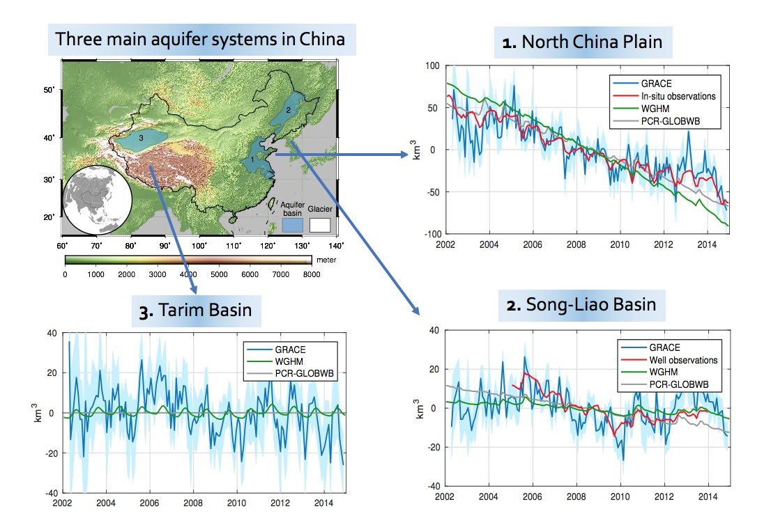
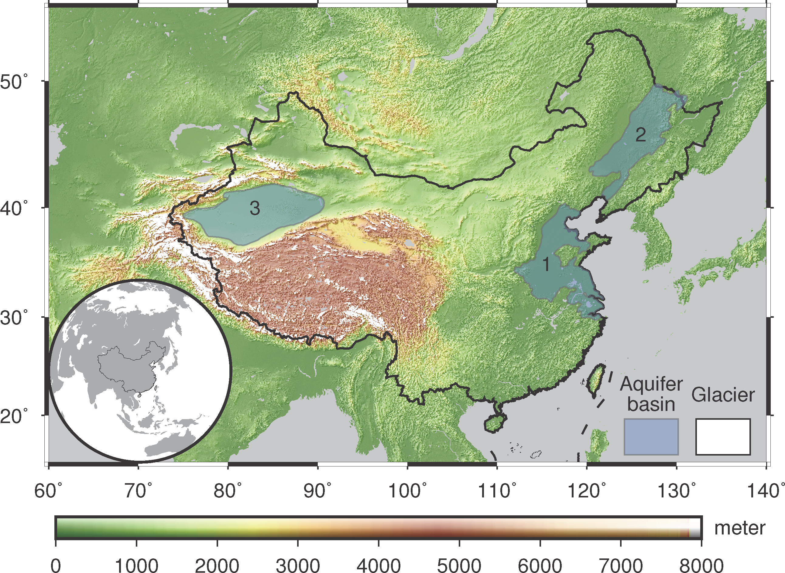
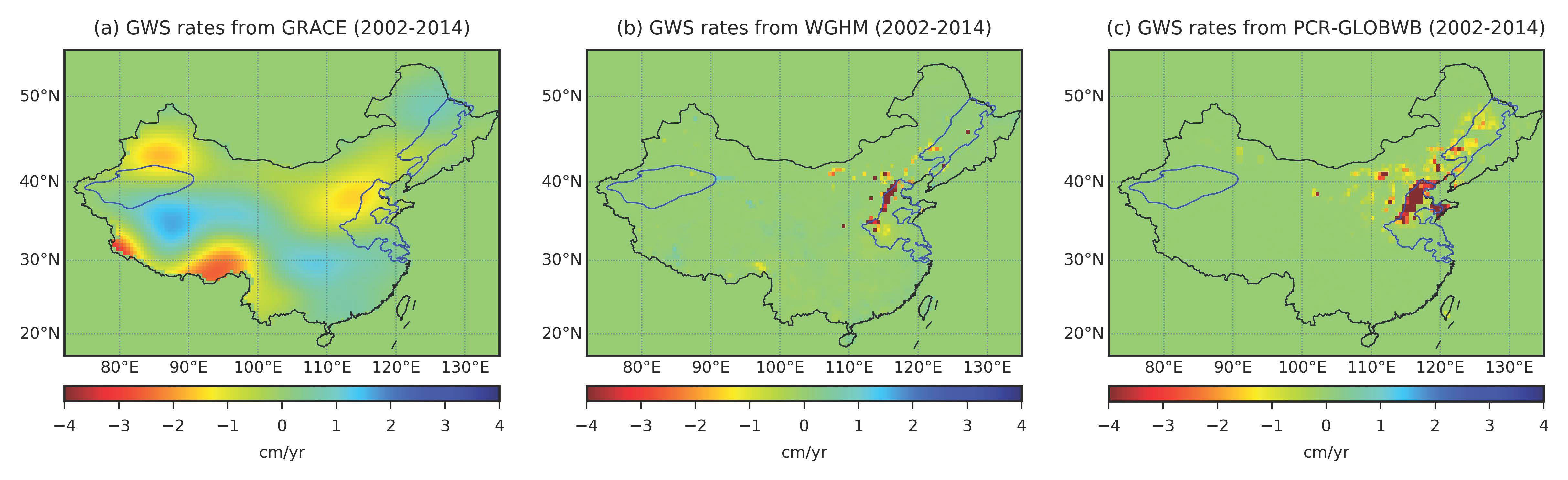
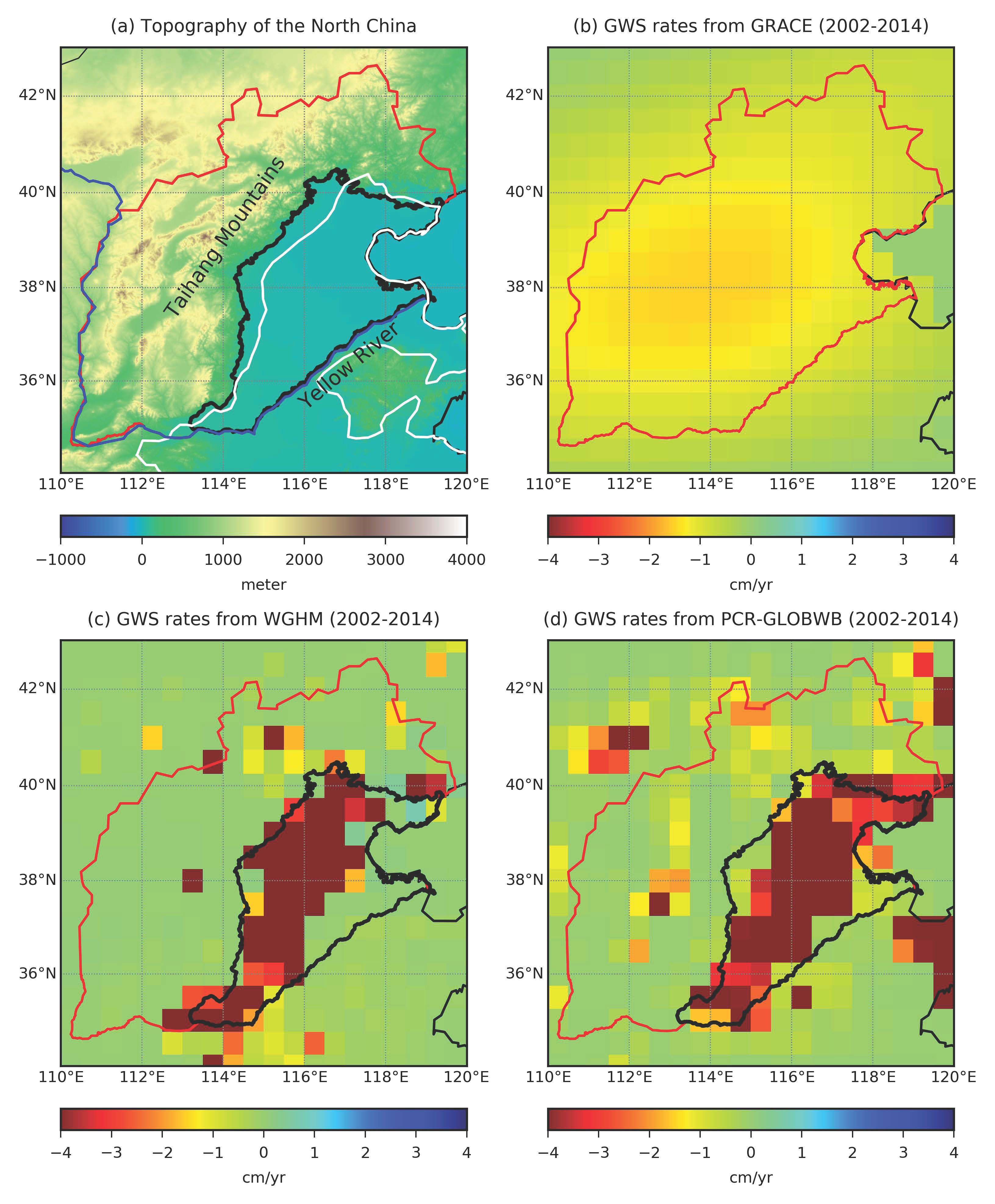
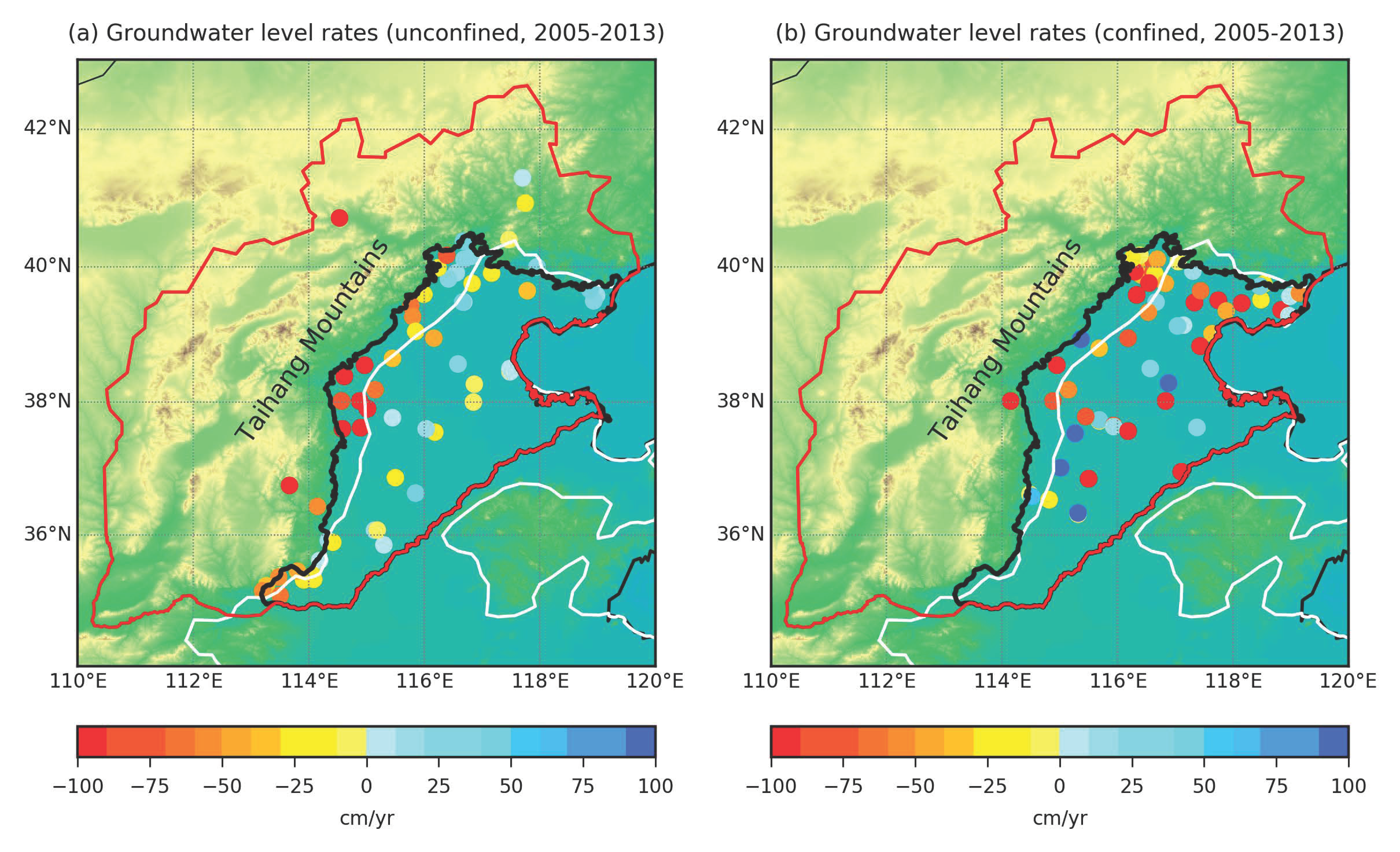
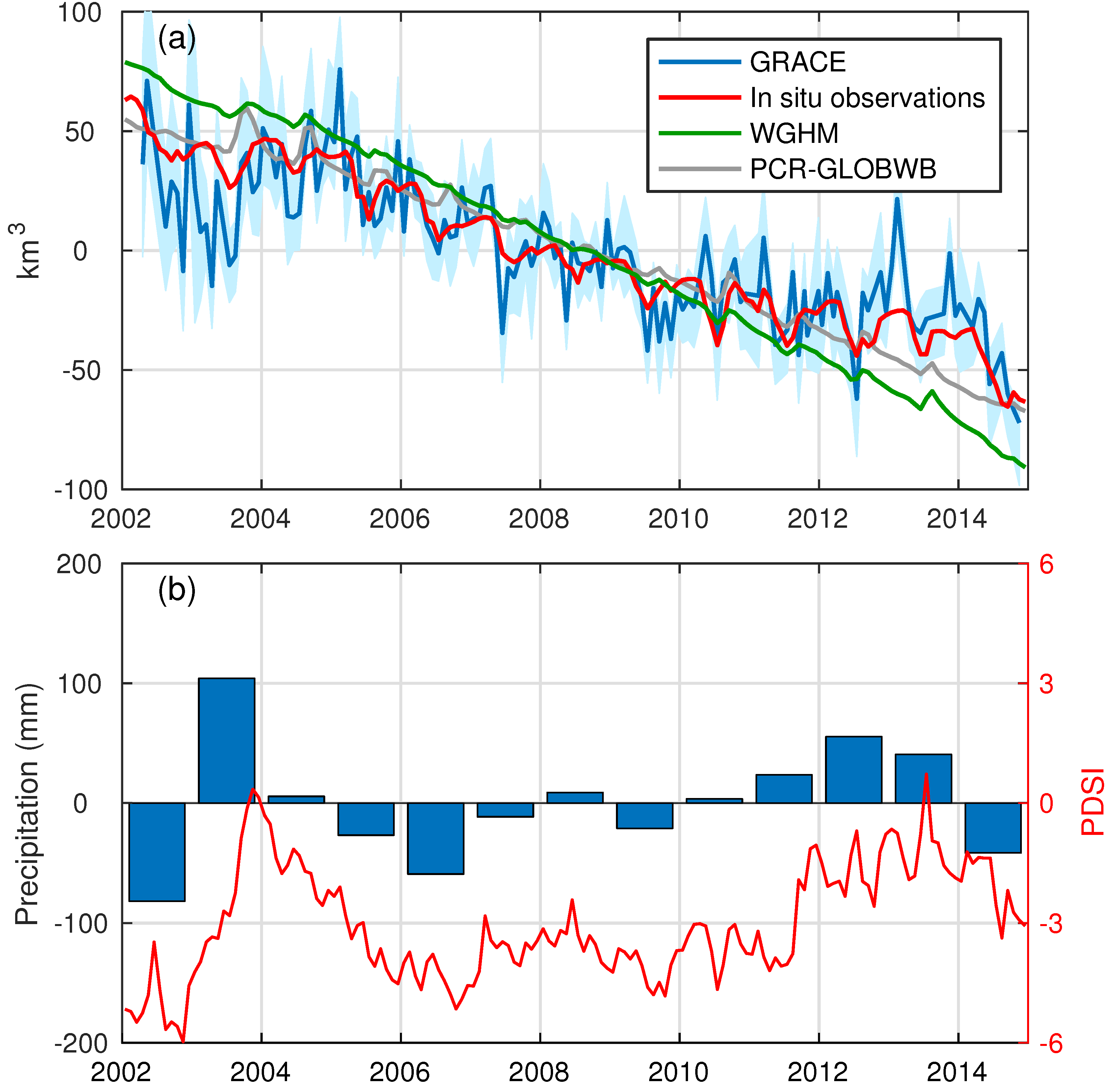
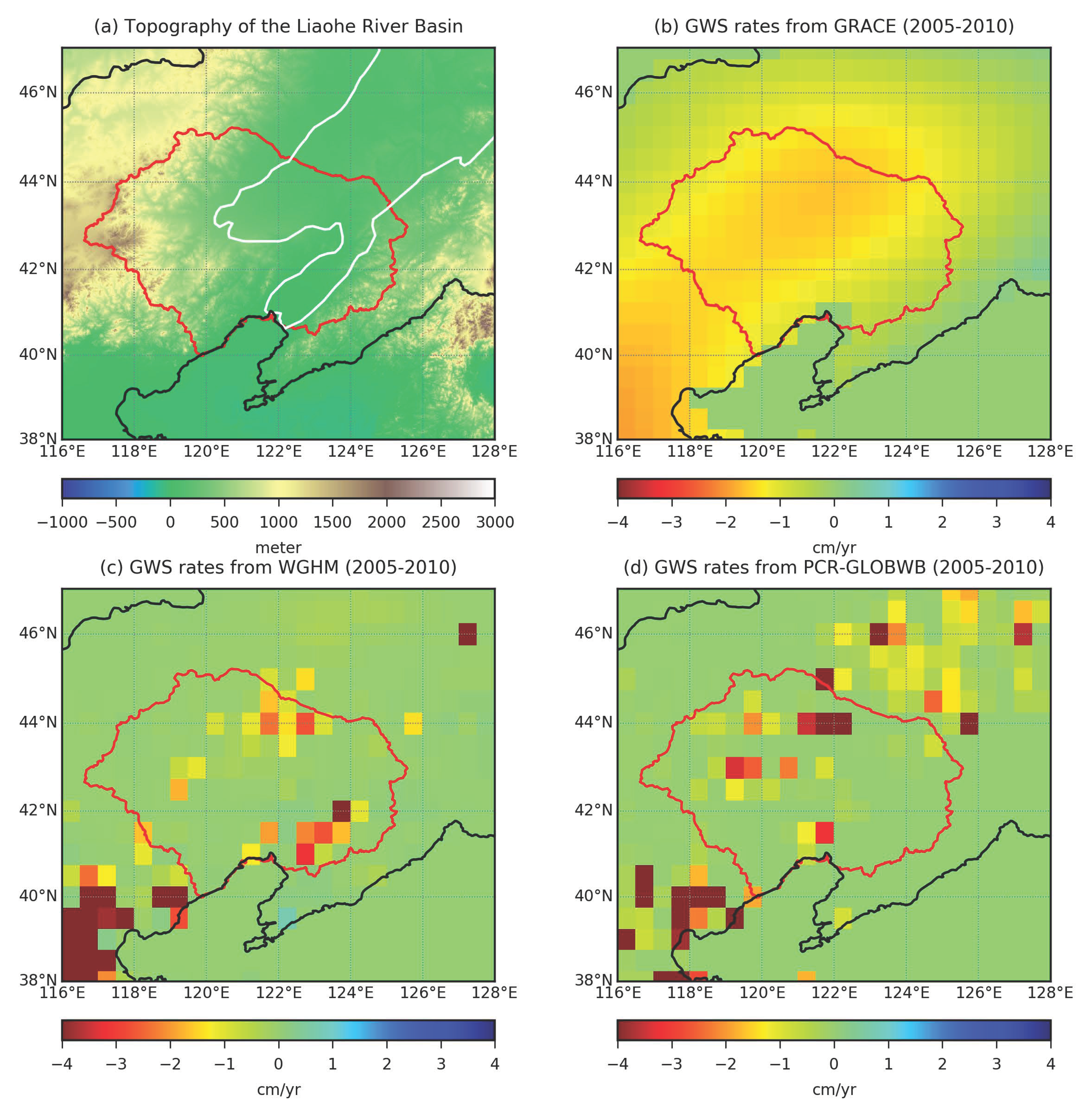
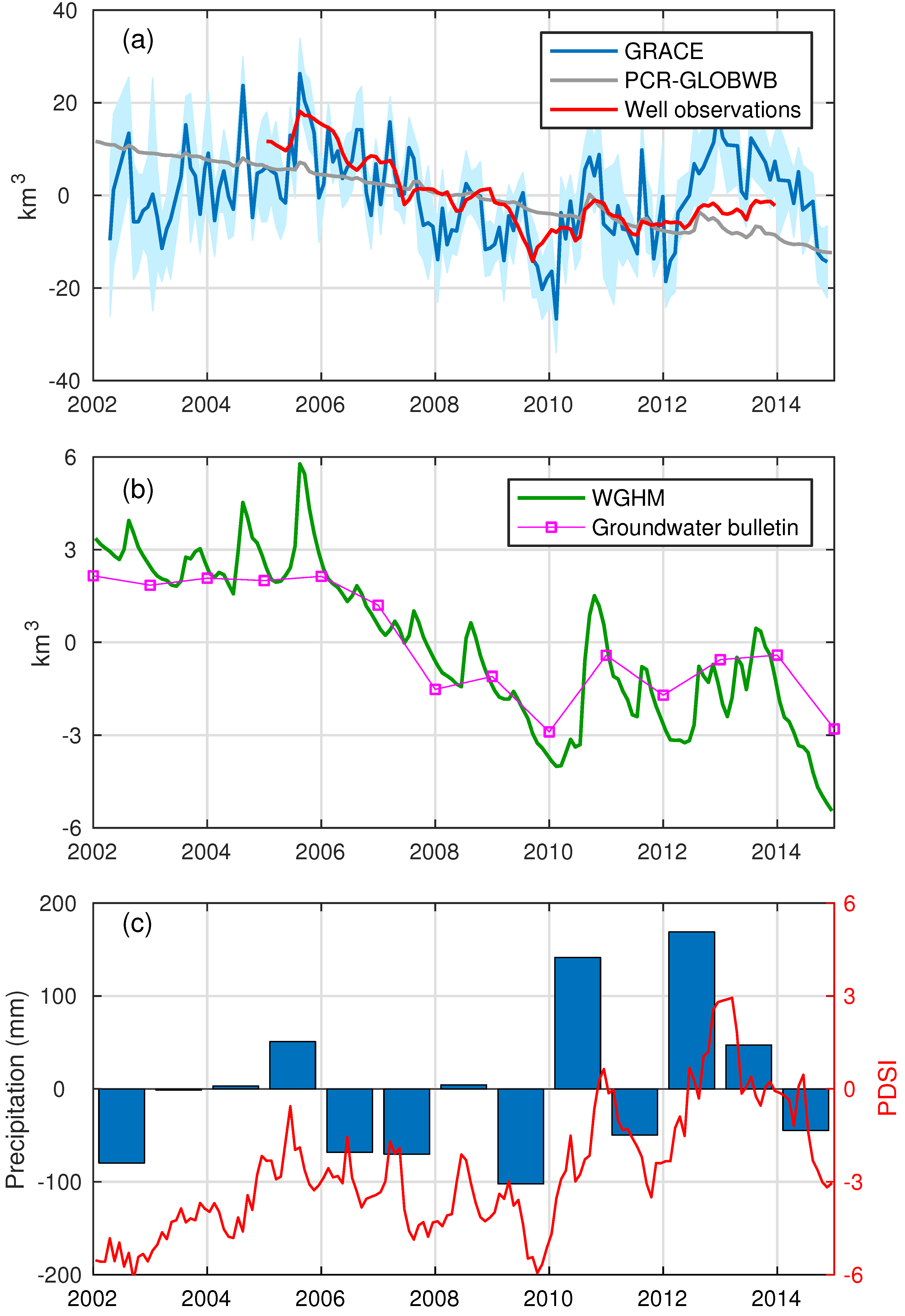
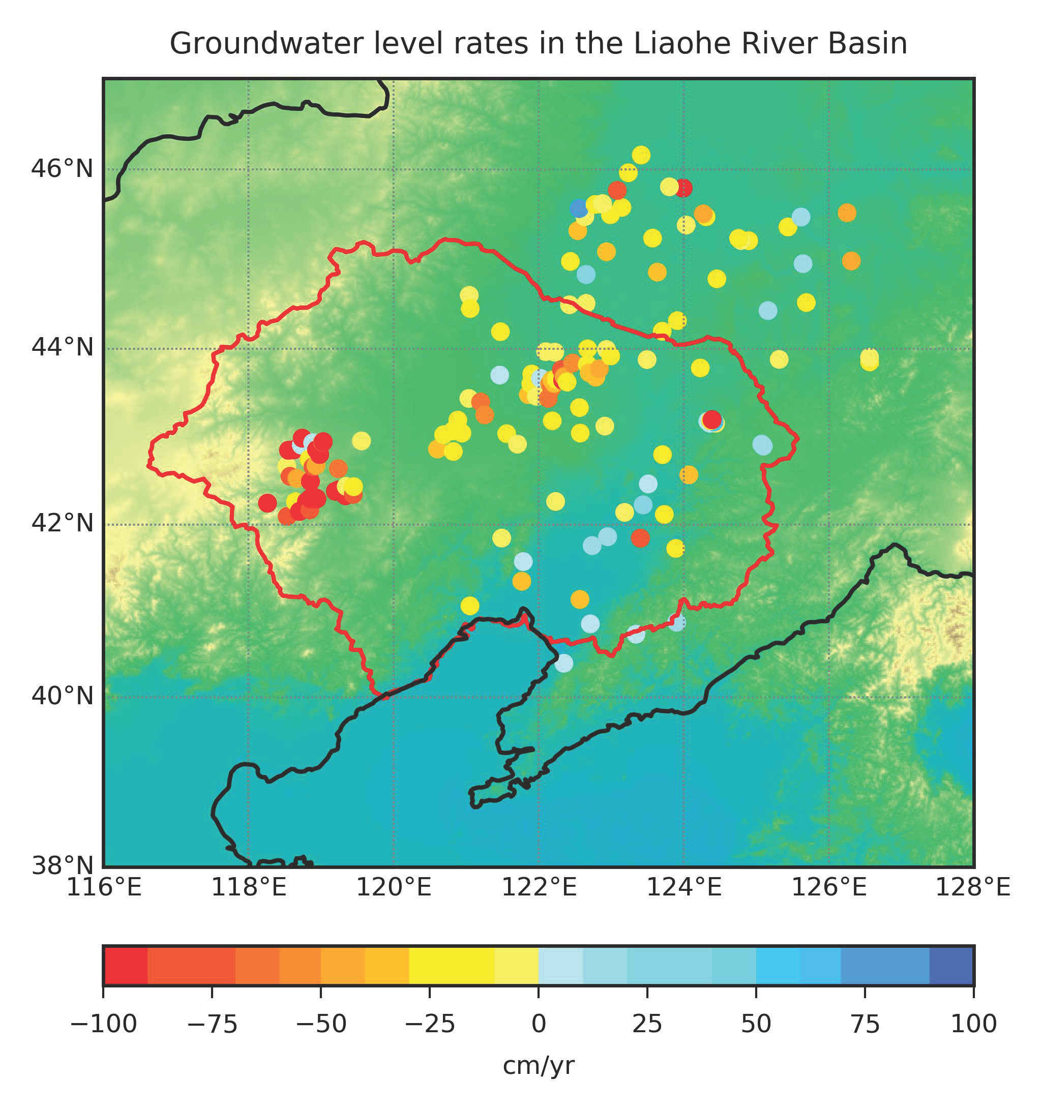
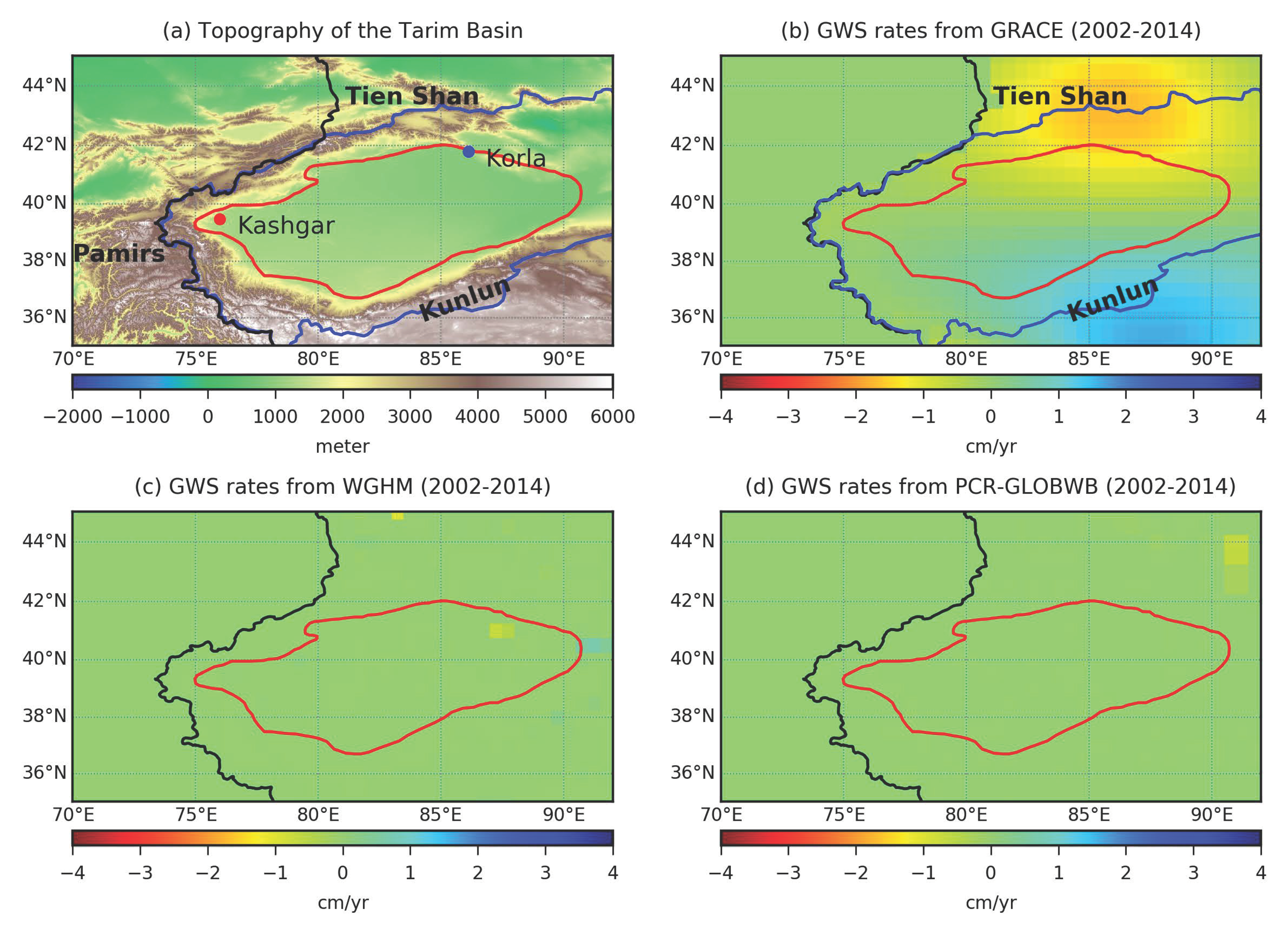
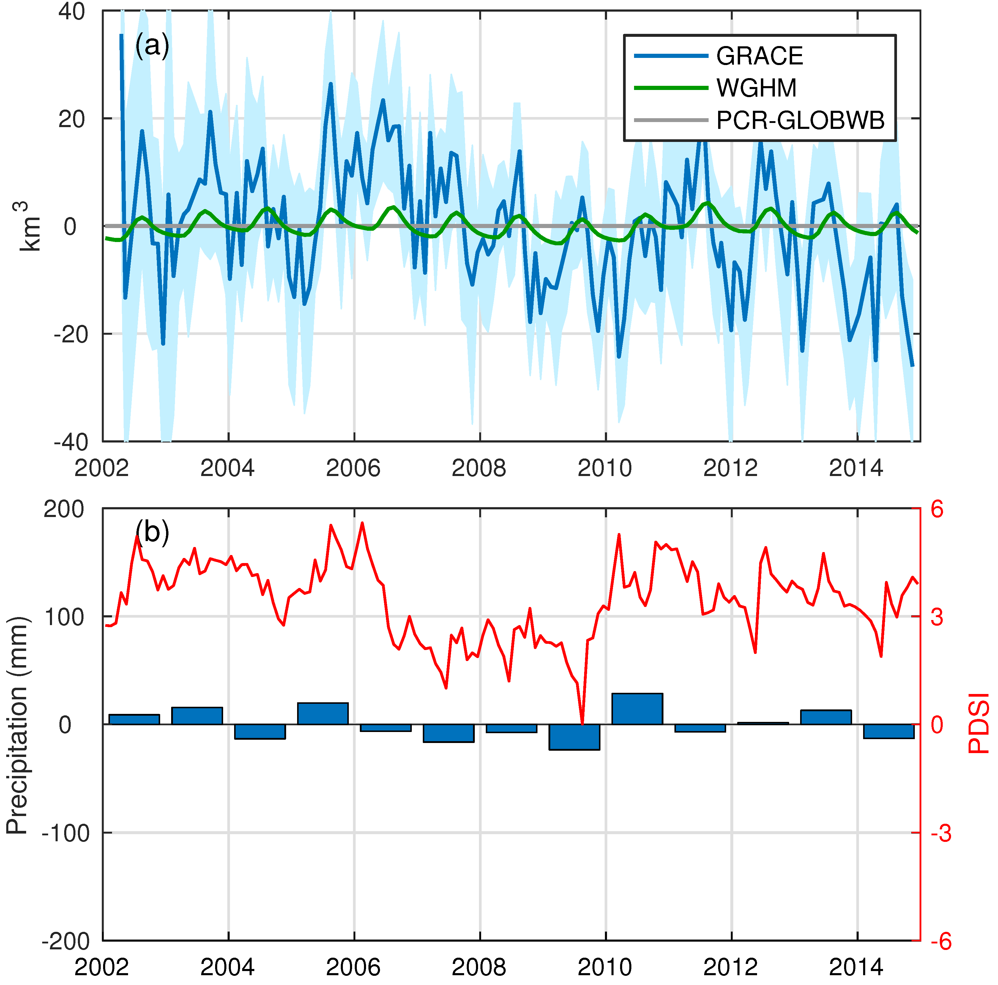
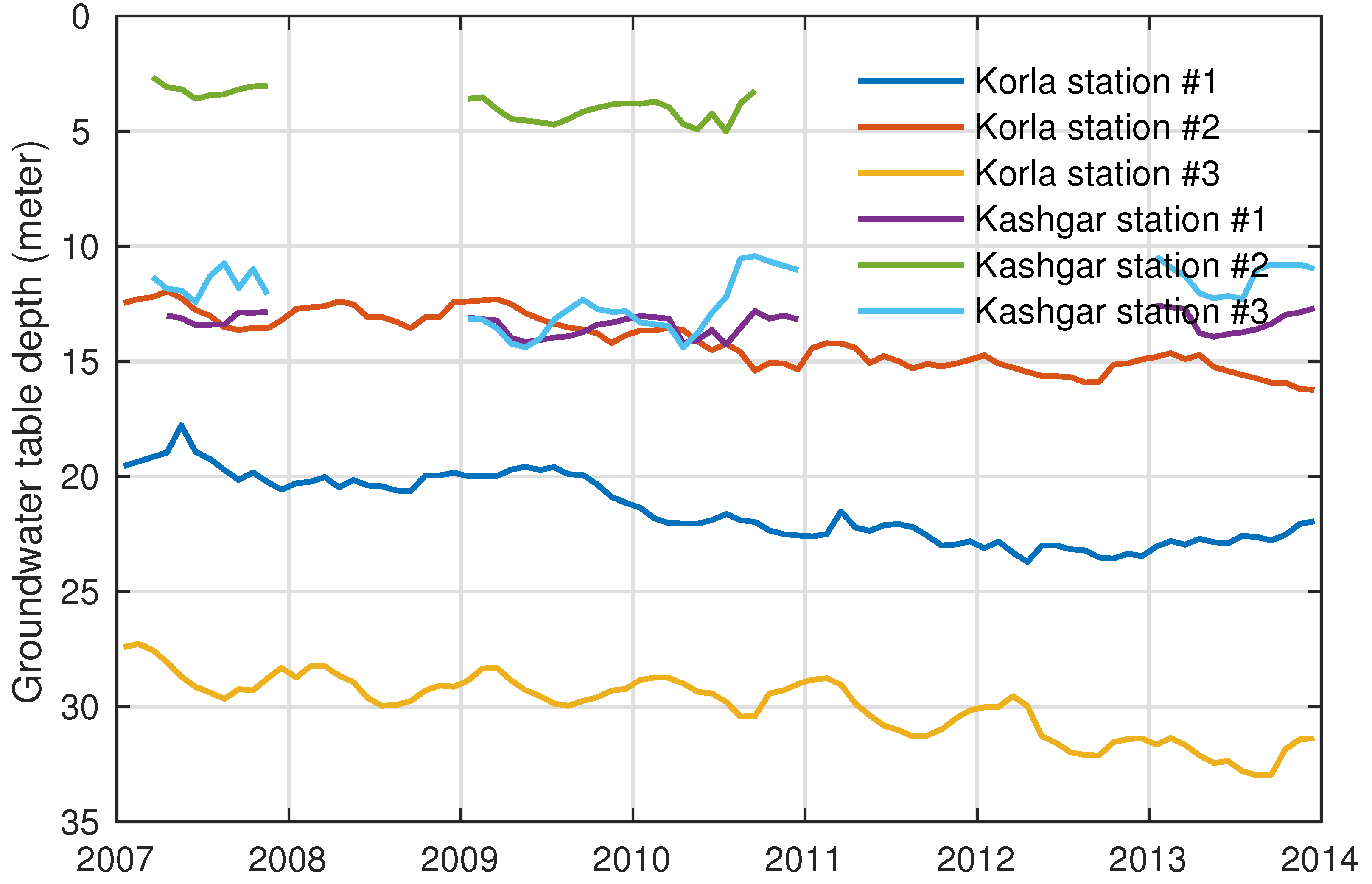
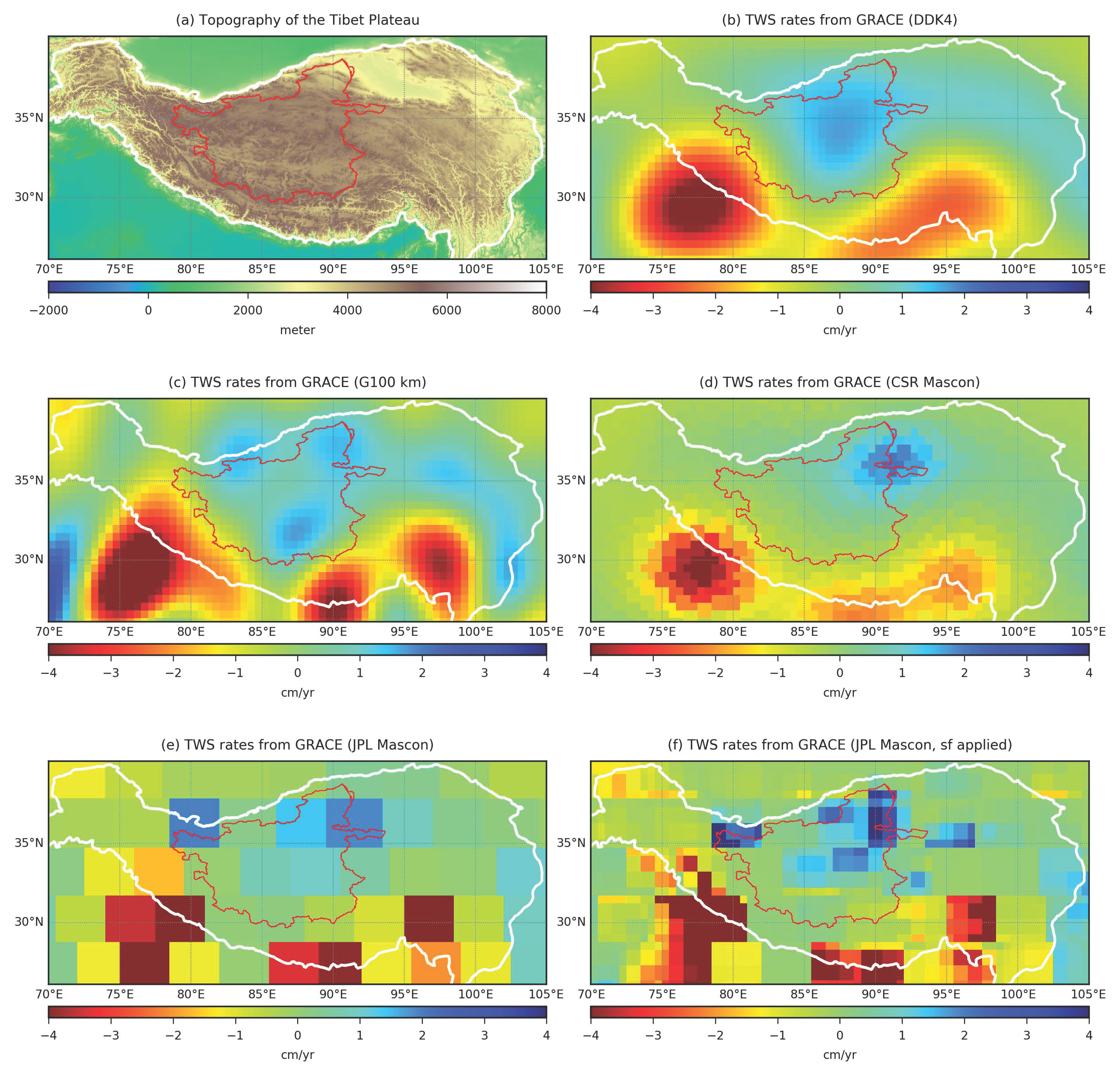
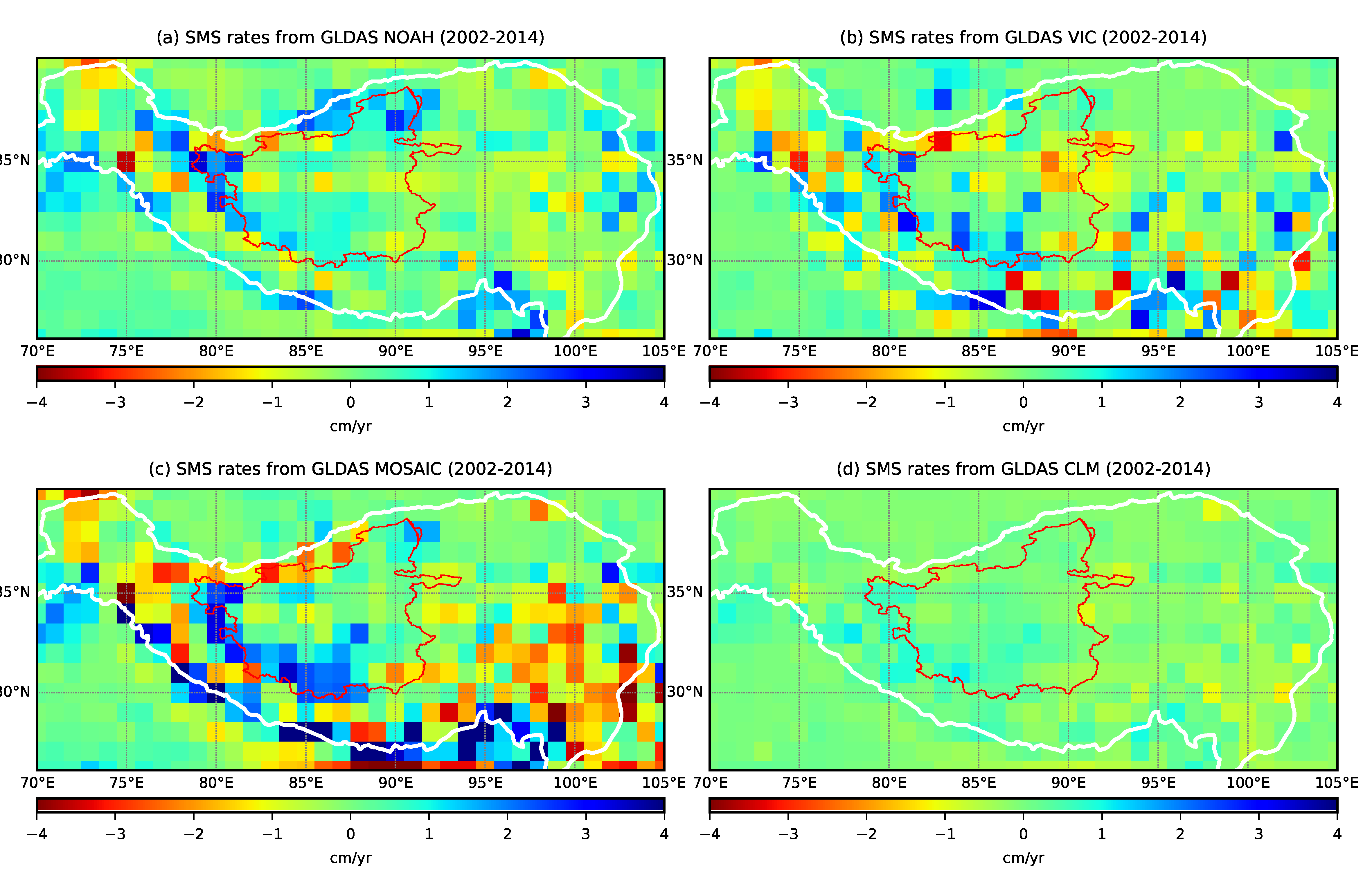
Table 1.
GWS rates (km3/yr) in the LRB based on GRACE, well observations, HMs and groundwater bulletins for 2005–2009 and 2002–2014.
Table 1.
GWS rates (km3/yr) in the LRB based on GRACE, well observations, HMs and groundwater bulletins for 2005–2009 and 2002–2014.
| GWS Rates | 2005–2009 | 2002–2014 |
|---|---|---|
| GRACE | −5.0 ± 1.2 | −0.5 ± 0.5 |
| Well observations | −5.1 ± 0.5 | - |
| PCR-GLOBWB | −2.0 ± 0.1 | −1.8 ± 0.1 |
| WGHM | −1.3 ± 0.1 | −0.6 ± 0.1 |
| Groundwater bulletins | −1.1 ± 0.2 | −0.4 ± 0.1 |
© 2018 by the authors. Licensee MDPI, Basel, Switzerland. This article is an open access article distributed under the terms and conditions of the Creative Commons Attribution (CC BY) license (http://creativecommons.org/licenses/by/4.0/).
Share and Cite
MDPI and ACS Style
Feng, W.; Shum, C.K.; Zhong, M.; Pan, Y. Groundwater Storage Changes in China from Satellite Gravity: An Overview. Remote Sens. 2018, 10, 674. https://doi.org/10.3390/rs10050674
AMA Style
Feng W, Shum CK, Zhong M, Pan Y. Groundwater Storage Changes in China from Satellite Gravity: An Overview. Remote Sensing. 2018; 10(5):674. https://doi.org/10.3390/rs10050674
Chicago/Turabian StyleFeng, Wei, C. K. Shum, Min Zhong, and Yun Pan. 2018. "Groundwater Storage Changes in China from Satellite Gravity: An Overview" Remote Sensing 10, no. 5: 674. https://doi.org/10.3390/rs10050674
Note that from the first issue of 2016, this journal uses article numbers instead of page numbers. See further details here.