Article

Groundwater Depletion in the West Liaohe River Basin, China and Its Implications Revealed by GRACE and In Situ Measurements

1
State Key Laboratory of Geodesy and Earth’s Dynamics, Institute of Geodesy and Geophysics, Chinese Academy of Sciences, Wuhan 430077, China
2
University of Chinese Academy of Sciences, Beijing 100049, China
*
Author to whom correspondence should be addressed.
Remote Sens. 2018, 10(4), 493; https://doi.org/10.3390/rs10040493
Submission received: 30 January 2018 / Revised: 7 March 2018 / Accepted: 19 March 2018 / Published: 21 March 2018
(This article belongs to the Special Issue Remote Sensing of Groundwater from River Basin to Global Scales)

Abstract

:
The West Liaohe River Basin (WLRB) is one of the most sensitive areas to climate change in China and an important grain production base in the Inner Mongolia Autonomous Region of China. Groundwater depletion in this region is becoming a critical issue. Here, we used the Gravity Recovery and Climate Experiment (GRACE) satellite data and in situ well observations to estimate groundwater storage (GWS) variations and discussed the driving factors of GWS changes in the WLRB. GRACE detects a GWS decline rate of −0.92 ± 0.49 km3/yr in the WLRB during 2005–2011, consistent with the estimate from in situ observations (−0.96 ± 0.19 km3/yr). This long-term GWS depletion is attributed to reduced precipitation and extensive groundwater overexploitation in the 2000s. Long-term groundwater level observations and reconstructed total water storage variations since 1980 show favorable agreement with precipitation anomalies at interannual timescales, both of which are significantly influenced by the El Niño-Southern Oscillation (ENSO). Generally, the WLRB receives more/less precipitation during the El Niño/La Niña periods. One of the strongest El Niño events on record in 1997–1998 and a subsequent strong La Niña drastically transform the climate of WLRB into a decade-long drought period, and accelerate the groundwater depletion in the WLRB after 1998. This study demonstrates the significance of integrating satellite observations, ground-based measurements, and climatological data for interpreting regional GWS changes from a long-term perspective.

Graphical Abstract

1. Introduction

Groundwater, as an important component of total terrestrial water storage (TWS), plays a key role in the global water cycle. Overuse of groundwater has caused various environmental problems in many places globally, e.g., desiccation of Lake Urmia, groundwater depletion in Northwest India and in the California Central Valley, and land subsidence in the North China Plain [1,2,3,4,5]. However, monitoring groundwater storage (GWS) is limited in many regions [6]. The absence of in situ monitoring well networks, low-quality observation data, and uncertainties in storage coefficients (i.e., specific yield, Sy) for translating groundwater level changes to groundwater storage variations restrict our knowledge of GWS changes [7,8].
Since its launch in 2002, the Gravity Recovery and Climate Experiment (GRACE) mission has provided a unique way to monitor TWS changes at a monthly scale and with a ~300 km footprint [9,10,11]. Furthermore, it can be used to estimate GWS changes when other TWS components can be removed or neglected. Many studies have compared the GRACE-derived GWS changes with independent in situ groundwater monitoring observations in many parts of the world. At the early stage, Rodell et al. [12] and Strassberg et al. [13] found good agreement between the GWS estimates from GRACE and the Global Land Data Assimilation System (GLDAS) model and those from in situ measurements in the Mississippi River basin and the High Plains Aquifer, USA, respectively. Subsequently, a number of studies have demonstrated the potential of GRACE to estimate GWS depletion in many regional basins, e.g., northwestern India [2,14,15,16,17], California’s Central Valley, USA [3,18,19], the North China Plain (NCP) [20,21,22], and the Middle East [23].
The West Liaohe River Basin (WLRB), which is located in Northeast China (Figure 1) and is known as the “Granary of Inner Mongolia”, is a major grain-producing region in China, with a rapidly growing population since 1950 [24,25]. The basin is in the transition zone between the Inner Mongolia Plateau and the Songliao Plain. The western part of the basin is the south of the Great Khingan Mountains, while the eastern part is the plain area (Figure 1). The WLRB is also the upstream portion of the Liaohe River and overlies a Quaternary loose rock pore aquifer, where extensive groundwater exploitation occurs. Land use in the WLRB is primarily grassland and cropland, with some tree covered land in the mountain region (Figure S1).
The WLRB is located in a semi-arid region, with an area of 136,000 km2. It has a continental climate that experiences dry and windy spring conditions, hot and humid summers, cool autumn conditions, and cold winters with little snow. As a semi-arid region, mean annual precipitation of the WLRB is 392 mm (1961 to 2015) and ranges from 260 to 540 mm. Annual precipitation is spatially variable, with less precipitation in the central plain (see Figure S2). About 80% of the precipitation occurs in summer (June to September) [26,27]; while the potential evaporation ranges from 1190 to 1860 mm, which greatly exceeds precipitation [24,28]. Since 1980, the surface flow of the West Liaohe River began to decline, and it nearly dried up since 2000 [24,29,30]. Water storage in lakes and reservoirs also decreased significantly after 1999 [31]. Groundwater has become a vital resource for agricultural, industrial, and domestic water use in the WLRB [32]. Most areas of the WLRB are equipped for irrigation with groundwater [32], which accounted for ~80% of the total water supply during 2005 to 2015. Thus, it is crucial to evaluate the state of groundwater resources in the WLRB for the development of sustainable agriculture and the preservation of terrestrial ecosystems. Groundwater level declines in the WLRB within the past two decades have been reported by several studies [33,34,35,36], e.g., with a rate of ~−0.18 m/yr from 1999 to 2010 [29]. Average groundwater levels in three main counties of the WLRB in 2006 decreased by 3.8 m, 2.8 m, and 1.9 m, respectively, when compared to those in 1978 [33]. However, quantitative evaluation of the GWS changes in the WLRB for the past decade was still limited.
In this study, we use GRACE, GLDAS land surface models (LSMs), and in situ measurements to evaluate the GWS changes during the GRACE era in the WLRB. Recent studies indicate that there has been an abrupt change in the annual precipitation in the WLRB since 1998, i.e., before the launch of GRACE satellites [37]. Therefore, longer period groundwater storage changes should be evaluated and interpreted. Based on the GRACE data and precipitation observations, we further reconstructed long-term TWS variations in the region prior to the GRACE era. The objective of this study was to address the following questions: (1) How can groundwater monitoring in the WLRB benefit from GRACE satellite data? (2) How do water storages change in response to human demand and climate forcing in the WLRB?

2. Data and Methods

TWS refers to all of the water stored in the land, including surface water, snow and ice, soil moisture, and groundwater. GWS anomalies (GWSA) can be estimated by subtracting surface reservoir storage anomalies (RESSA), snow water equivalent storage anomalies (SWESA), and soil moisture storage anomalies (SMSA) from the GRACE-derived TWS anomalies (TWSA):
GWSA = TWSA RESSA SWESA SMSA
where RESSA can be estimated from in situ monitoring and is negligible in some cases; and, SWESA and SMSA can be estimated by hydrological models or in situ observations. In this study, in situ groundwater level anomalies (GWLA) were used to validate the GWSA derived from GRACE and ancillary data. In addition, precipitation data and climate indices were used to assess the impact of climate variability on TWS/GWS changes. A summary of the datasets that were used in this study can be found in Table 1.

2.1. TWSA Derived from GRACE

We used the GRACE Mascons solution that was provided by the Center for Space Research (CSR), the University of Texas at Austin, to derive TWSA [38]. Both mascon and CSR RL05 spherical harmonic products were based on the same GRACE level-1 observations, also with C20 replacement, degree 1 corrections, and glacial isostatic adjustment (GIA) corrections. CSR Mascons (CSR-M) are provided with a 0.5 degree spatial resolution. The regularization constraint on mascon solutions is derived from original GRACE information with no empirical filtering post-processing [38]. Some studies have concluded that, although no empirical post-processing is required, mascon solutions can still provide comparable TWSA estimates as traditional spherical harmonic products [38,39].

2.2. SMSA+SWESA Derived from GLDAS LSMs

We used four versions of LSMs from GLDAS to estimate SMSA and SWESA, i.e., Noah [40], CLM [41], MOSAIC [42], and VIC [43]. The GLDAS LSMs were developed by the National Aeronautics and Space Administration (NASA) and the National Oceanic and Atmospheric Administration (NOAA). Constrained by ground- and space-based observations, the GLDAS LSMs can simulate the optimal fields of land surface states and fluxes [44]. Simulated SMSA from Noah, MOSAIC, VIC, and CLM include changes in soil water contents with depths of 2.0 m, 3.4 m, 3.5 m, and 1.9 m, respectively.

2.3. GWSA from In Situ Observations

The groundwater monitoring well observations were obtained from the groundwater level yearbook that was published by the China Institute of Geological Environment Monitoring (CIGEM) [45] and from the Hydrological Bureau of Inner Mongolia (HBIM) for the period of 2005–2015. The mean groundwater level anomalies (GWLA) from a total of 122 observation wells and the GWLA from each well were shown in Figure S3. Some of the raw groundwater level data are highly inaccurate with variability between consecutive months greater than 2 m in some records, which were eliminated during the preprocessing stage. The month-to-month number of available well records varied from 45 to 103. The GWSA from ground well observations are calculated as follows [7,46]:
G W S A = j N S j W j h j / j N W j
where Sj is the Sy value of each grid cell j; N represents the total number of grid cells; Wj is the weight of each grid cell (the cosine of the latitude of the corresponding cell); and, ∆hj refers to the mean value of the groundwater level variations in each grid cell. We divided the study region into a 1° × 1° mesh as Strassberg et al. [13]. In this study, a mean Sy value of 0.042, determined by pumping tests, was used to translate groundwater level changes to water storage changes, as suggested by the Songliao Water Resources Commission (SLWRC) [47].
Besides the monthly groundwater level observations from CIGEM and HBIM, we also collected annual mean groundwater levels in the WLRB for the period of 1980–2010 from Xu [29] and for the period of 1997–2015 from the annual Water Resources Bulletin (WRB) released by the HBIM [32]. Then, we derived a long-term time series of annual GWLA from 1980 to 2015. Note that we used the mean values of annual groundwater levels from the two sources during the overlap period (1997–2010).

2.4. RESSA from Ground Measurements

To estimate GWSA in the WLRB from GRACE-derived TWSA, RESSA, as a potentially important TWS component in some regions, should be taken into account. For the WLRB, annual mean storage data of surface water were collected from the WRB, as published by the HBIM [32]. The RESSA trend was −0.05 km3/yr from 2005 to 2011, and −0.02 km3/yr from 2005 to 2015. Although the contribution of RESSA is rather small, we still removed it from the GRACE-derived TWSA to obtain GWSA.

2.5. Precipitation Data and Climate Indices

Gridded precipitation data over the study region were obtained from the China Meteorological Data Service Center (CMDC). These gridded data were obtained by spatial interpolation of precipitation observations from 2472 weather stations with monthly and daily temporal resolutions and 0.5° × 0.5° spatial resolution over all of China. Additionally, we used NOAA’s Oceanic Niño Index (ONI) to represent the El Niño-Southern Oscillation (ENSO) variability. Positive ONI values represent the warm ENSO phase (i.e., El Niño), while negative ONI values represent the cold ENSO phase (i.e., La Niña).

2.6. Climate-Driven Water Storage Variability

To further assess the impact of climate variability on TWS and better interpret GWS changes in the WLRB, a long-term water storage variation time series from 1980 to 2013 was reconstructed based on long-term precipitation data and eleven-year GRACE CSR-M data. The details on the reconstruction method of climate-driven sub-decadal water storage variability can be found in [48,49]. In brief, first, the effect of one day’s precipitation flux to later days can be expressed by an exponential decay filter:
f ( t ) = { 0 ,   t < 0 e t τ τ ,   t 0
where t is time and τ is a decay parameter which is calibrated. Then, filtered daily time series was averaged to the monthly resolution using an arithmetic mean. As the exponential decay filtered daily precipitation is highly correlated with interannual and subseasonal TWSA [49], the precipitation-driven TWSA was formulated as following:
TWSA r e c = β · P i n t e r + s u b s e a s τ
where TWSA r e c is the reconstructed nonseasonal and detrended TWS variations; P i n t e r + s u b s e a s τ corresponds to the deseasoned and detrended filtered precipitation. The parameters τ and β were calibrated by using daily precipitation from CMDC and TWSA i n t e r + s u b s e a s derived from deseasoned and detrended GRACE-derived TWSA. Because the precipitation data from CMDC with daily resolution are available until 2013, we reconstructed the TWSA time series from 1980 to 2013. In the original TWSA reconstruction by Humphrey et al. [49], temperature change was also considered in addition to precipitation. In this study, however, we only used precipitation data because temperature has less effect on TWSA (Vincent Humphrey, personal communication).

2.7. Regression Analysis between Groundwater Flux and Precipitation Anomalies

To investigate the effect of precipitation anomalies on groundwater storage changes, we constructed a linear relationship between the variations in precipitation and GWS, as follows [50]:
F = a P + b
where F is annual groundwater flux (GWF, GWS change between two successive years, in km3/yr); ∆P is annual precipitation anomalies relative to the study period, which is multiplied by the area of WLRB to convert it to km3/yr. In addition, a and b are the parameters that are calibrated by regression analysis: a is the ratio of groundwater flux to precipitation anomalies (dimensionless); b is the residual that cannot be explained by precipitation anomalies, which can be attributed to anthropogenic effects.

2.8. Uncertainty Assessment

The TWSA uncertainty was estimated based on the approach suggested by Landerer and Swenson [51] and Scanlon et al. [39]. We first obtained the residuals by removing the linear trend and seasonal components from TWSA time series. The interannual signals were further removed by fitting a 13-month moving average to the residuals because they also contributed significantly to the TWSA in the WLRB. The RMS of the residuals was used as the measurement uncertainty in TWSA. Our uncertainty estimate was relatively conservative, as the residuals would still contain subseasonal signals. The uncertainty in SMSA+SWESA was estimated from the standard deviation (STD) among the time series that were produced by the four GLDAS models.
We computed the trend in GWSA based on GRACE-derived TWSA and mean SMSA+SWESA from the four GLDAS models (Noah, CLM, Mosaic and VIC). The GWS trend estimates were calculated using unweighted least squares to fit a linear trend, plus annual and semiannual sinusoids to the time series of GWSA [15]. The uncertainty in GWS trend was also estimated when considering the error propagation law during the least squares fit and uncertainties in TWSA and SMSA+SWESA. Uncertainty in Sy was estimated to be ±20%, which was used to estimate the uncertainty in the GWS trend from in situ observations.

3. Results

3.1. GWSA from 2005 to 2015

Figure 2a shows the time series of TWSA estimated from GRACE, and mean SMSA+SWESA from four GLDAS LSMs. The shadows show the uncertainties in TWSA (±1.49 cm) and SMSA+SWESA (±0.72 cm). TWSA uncertainty is close to the global mean uncertainty value of TWSA (~2 cm), as suggested by CSR. As shown in Figure 2a, TWSA decreases at a rate of −1.26 ± 0.49 cm/yr from 2005 to 2009 continuously, and then shows relatively large interannual variability from 2010 to 2013, and decreases rapidly again after 2013. The SMSA+SWESA show comparable interannual changes as TWSA from 2005 to 2015. Both TWSA and SMSA+SWESA show two peaks at the end of 2010 and 2012.
Figure 2b shows the time series of GWSA based on GRACE and in situ measurements. During the drought period from 2005 to 2011, the GRACE-derived GWSA in the WLRB declined rapidly at a rate of −0.92 ± 0.49 km3/yr (i.e., −0.68 ± 0.36 cm/yr in equivalent water height (EWH)). For the same period, the GWSA trend from in situ measurements is −0.96 ± 0.19 km3/yr (i.e., −0.70 ± 0.14 cm/yr EWH), which is in good agreement with the GRACE-derived estimate. The time series from GRACE and in situ observations also compare favorably before 2011.
For the whole study period of 2005–2015, GRACE-derived GWSA in the WLRB, as declined at a rate of −0.43 ± 0.26 km3/yr (i.e., −0.32 ± 0.18 cm/yr in EWH), significantly less than the rate from 2005 to 2011. The obvious interannual signals during 2012–2015 result in the difference of GWS rates between the two periods. The GWS rate from well observations is −0.73 ± 0.15 km3/yr from 2005 to 2015.
Figure 2c shows annual precipitation anomalies, annual GWSA results from GRACE, in situ measurements, and WRB. In addition to the obvious long-term GWS depletion for the entire time period, the GRACE-derived GWSA increased in 2012 and 2013 in response to more precipitation in 2012, which is also shown by the GWSA from WRB, but with relatively lower magnitude. The continuous GWS decrease that as observed by in situ measurements also slows down from 2011 to 2013. For the years of 2014 and 2015, the GRACE-derived GWSA decreased rapidly again.

3.2. GWSA from 1980 to 2015

Both GRACE and in situ measurements show significant groundwater depletion in the WLRB from 2005 to 2011. Over a longer time period, Figure 3a shows the mean annual groundwater table changes in the WLRB which declined slowly from 1980 to 1998, and declined more rapidly after 1998. These data indicate that groundwater levels in the WLRB had decreased before the GRACE era. As shown in Figure 4a, the WLRB experienced a long-term drying climate and had the lowest average annual precipitation since 1980 for the period of 1999–2009 [37]. The average annual precipitation during this period decreased by 15% relative to the average annual precipitation from 1961 to 2015. The turning point in precipitation anomalies in 1998 is consistent with the occurrence of one of the largest El Niño events on record in 1997–1998, followed by the long-term drought (Figure 4a).
Although the WLRB did not experience significant droughts before 1998, annual groundwater exploitation increased continuously due to extension of crop cultivation and expanding irrigation (Figure 3b) [52]. Annual groundwater exploitation also shows a jump in 1998, and remains high since then. This feature also agrees well with the occurrence of the 1997–1998 El Niño event and the following long-term precipitation deficit. This jump in the signal is consistent with the acceleration in groundwater level decline after 1998 (Figure 3a). Although the annual water consumption statistics (including agricultural, industrial, and urban use) in the WLRB are only available after 1998, we find that ~80% of water consumption in this region is from groundwater exploitation during 1998–2015 (Figure 3c), consistent with the continuous groundwater level decline (Figure 3a).
Relative to the average of precipitation from 1980 to 2015, precipitation anomalies are positive in most of years prior to 1998, but negative for the continuous eleven years from 1999 to 2009 (Figure 4a). Time series of ONI highlights the strong El Niño/La Niña years from 1980 to 2015 (Figure 4). Precipitation anomalies in the WLRB agree well with ENSO events (Figure 4a). For example, annual precipitation increases significantly during the three El Niño periods (e.g., 1987–1988, 1991–1992, and 1997–1998). In contrast, annual precipitation decreases generally during the La Niña periods (e.g., 1988–1989, 1998–2000, 2007–2008, and 2010–2011).
The reconstructed climate-driven TWSA and detrended mean GWLA in the WLRB show similar interannual changes during 1980–2013 (Figure 4b). Both ONI and reconstructed TWSA were applied with a Vondrak filter to exclude the high frequency signal of less than one year [53,54]. Generally, both show significant increases during El Niño events and decreases during La Niña events. TWSA and GWLA reach their maxima in 1998, consistent with the extreme precipitation increase in this year due to the strong 1997–1998 El Niño event. After the abrupt precipitation increase in 1998, GWLA and TWSA decreased from 1999 to 2010, consistent with the long-term precipitation deficit associated with continuous La Niña periods.

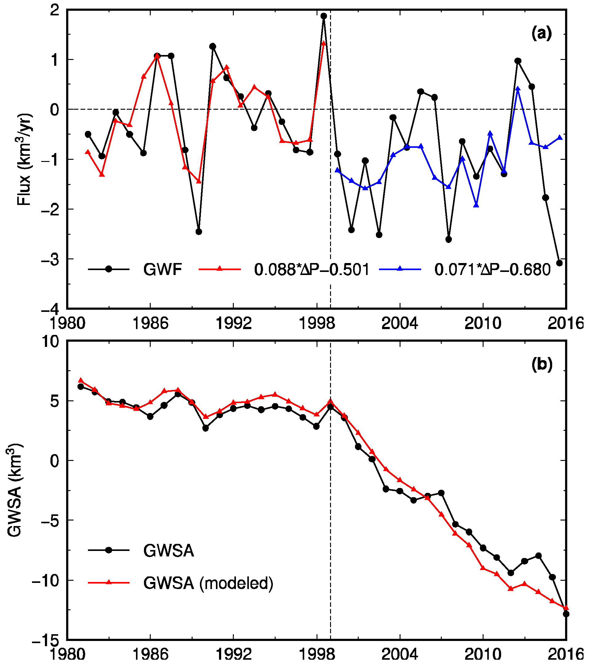
3.3. Groundwater Flux (GWF) from 1980 to 2015

The linear relationship between GWF and precipitation anomalies were constructed using the regression analysis method in Section 2.7. The difference of groundwater levels between two successive years was multiplied with the mean Sy to retrieve the time series of mean GWF over the WLRB. Note that the negative GWF values represent GWS depletion when compared to the previous year; and vice versa. More negative GWF values after 1998 indicate a long-term GWS depletion in the WLRB (Figure 5a), consistent with the results in Figure 3a. Due to distinct features for GWLA before and after 1998, we split the time period into two parts, i.e., 1980–1998 and 1998–2015, and constructed a linear relationship for these two periods.
For the first time period, the GWF is more sensitive to precipitation anomalies. The ratio parameter a in Equation (5) for the period 1980–1998 is 0.088. It indicates that 1 km3 (i.e., ~7.35 mm over the WLRB) of precipitation anomalies can cause a groundwater storage change of 0.088 km3. In other words, ~9% of annual precipitation recharges the aquifers in the WLRB. This ratio is highly consistent with the mean precipitation infiltration coefficient from 1988 to 1997 (i.e., 0.087) in the WLRB estimated by Xu [29]. This good agreement confirms that the linear relationship in this time period is reasonable. Based on Equation (5), we assume that the anthropogenic effect is constant and can be estimated by the parameter b. The anthropogenic contribution to GWF (i.e., discharge of aquifer) is estimated to be −0.501 km3/yr. The coefficient of determination R2 between GWF and regression-modeled GWF reaches 0.64; while the RMS between them is 0.601 km3/yr. Good agreement between the GWF and regression-modeled GWF also indicates that it is reasonable to assume a linear relationship between GWF and precipitation anomalies.
For the second time period, however, precipitation anomalies contribute less to GWF, with a ratio of 0.071. The R2 between GWF and regression-modeled GWF is only 0.22, which indicates that the linear relationship between the GWF and precipitation is relatively weak for this time period. Figure 5a shows poor agreement between GWF and regression-modeled GWF for the period of 1998–2015.
The discrepancy from 1998 to 2015 indicates that there are still some limitations in this linear regression analysis method. First, we do not consider the time lag of groundwater change in response to precipitation, which could take several months or even more than one year. Because the groundwater table in the WLRB was relatively shallow during 1980–1998 (i.e., 2–3 m, shown in Figure 3a), the effect of the delayed response of groundwater is limited. From 1998 to 2015, however, the groundwater table reaches a depth of 5–6 m. Thus, the time lag might be non-negligible, even on interannual time scales. This could be one of the reasons to explain the discrepancy during 1998–2015. Second, in this method, we assume a constant anthropogenic contribution to groundwater, i.e., a fixed annual groundwater exploitation amount. Under the long-term drying climate in the WLRB since 1998, however, the annual groundwater exploitation amount probably changes over time. It can also explain the poor agreement between GWF and regression-modeled GWF from 1998 to 2015.
Long-term GWSA was compared with the modeled GWSA (Figure 5b). Note that the integral of the regression-modeled GWF with respect to time was computed for the aforementioned two time periods to derive the modeled GWSA from 1980 to 2015. The two time series are highly correlated (R2 = 0.99) (Figure 5b), which indicates that the linear regression analysis method can be used to model the GWSA very well. The trends in GWSA and modeled GWSA from 1980 to 1998 are −0.10 km3/yr and −0.06 km3/yr, respectively; while the trends during the second time period are −0.87 km3/yr and −1.04 km3/yr, respectively. Similar to the results in Figure 5a, the time series of GWSA and modeled GWSA agree with each other better for the period of 1980–1998, with consistent interannual fluctuations. From 1998 to 2015, however, some interannual signals in GWSA, e.g., in the 2000s, cannot be modeled well due to the limitations in the linear regression method that are mentioned before.

4. Discussion

4.1. Interannual Variablity of GWS from 2012 to 2015

GRACE-derived GWSA shows a significant increase in GWS from 2012 to 2013 followed by a rapid decline in 2014 and 2015. This interannual variability cannot be found from in situ well observations (Figure 2b). The GWS increase in 2012 and 2013 can be attributed to the abnormal precipitation increase in 2012 (Figure 2c). The statistics from the WRB also show a similar GWS increase in 2012 and 2013 as GRACE, but with lower amplitude (Figure 2c). One possible reason for missing interannual variability in ground observations is the uneven distribution of monitoring wells. As shown in Figure 1, there are few wells in the mountain area and the upstream area of the plain. In addition, in this work, we used a mean Sy (i.e., 0.042) from the SLWRC [47] and failed to derive the spatial information of Sy in the WLRB. It would also cause uncertainties during the estimation of in situ GWSA.
There are uncertainties in GRACE-derived GWSA too. The area of the WLRB is slightly less than the GRACE nominal resolution, i.e, ~200,000 km2. But, some studies have concluded that GRACE is able to detect water storage changes in localized regions with areas below GRACE resolution if the signal magnitude is sufficiently large [56,57]. In addition, simulated SMSA+SWESA from global GLDAS LSMs at small spatial scales, such as the WLRB, is likely to be underestimated or overestimated. Nevertheless, interannual fluctuations in GRACE-derived GWSA from 2012 to 2015 are still statistically significant (Figure 2b,c). The time series of GWSA based on other GRACE products and methods also show similar interannual variability from 2012 to 2015 (not shown), which confirm this interannual signal that is shown in Figure 2b,c.

4.2. Uncertainties in GRACE-Derived GWS Rates

Based on the law of error propagation and the uncertainties in GRACE-derived TWSA and model-based SMSA+SWESA, the uncertainty in GRACE-based GWS rate in the WLRB is 0.49 km3/yr and 0.26 km3/yr, respectively, for the time period 2005–2011 and 2005–2015. As the area of the LRB is less than the GRACE nominal spatial resolution, we further compared the results based on various GRACE solutions and methods to validate the GWS depletion signal in the WLRB.
As shown in Table 2, the GWS rate estimates during 2005–2015 derived from different GRACE solutions varied from −0.43 km3/yr to −0.65 km3/yr, agreeing with each other with respect to the error bounds. Additionally, all of the GRACE solutions show a higher GWS depletion rate during 2005–2011 than that for the entire period 2005–2015. For the period 2005–2011, GWS rates from various GRACE solutions show some variability, ranging from −0.84 km3/yr to −1.67 km3/yr, but still agree with each other within the uncertainty envelope. The GWS rate estimated from GRACE CSR Mascons and used in this study is −0.92 ± 0.49 km3/yr during 2005–2011, most consistent with the estimate from in situ measurements (−0.96 ± 0.19 km3/yr). The comparison of various GRACE solutions confirmed the significant depletion of GWS occurred in the WLRB.

4.3. Comparison with Other Studies

Xu [29] constructed a distributed hydrological model for basin scale water cycle simulation (MODCYCLE) over the WLRB for 1988–1997 and 2001–2010. The input data contained basic geographic information data, meteorological observations (e.g., precipitation, air temperature, wind speed, etc.), soil parameters, groundwater level data, and water supply and use data, etc. Based on the MODCYCLE model over the WLRB, the mean recharge to the unconfined aquifers was 3.94 km3/yr, and the mean discharge from the unconfined aquifers was 5.17 km3/yr from 2001 to 2010. Thus, the GWS depletion rate for 2001–2010 is −1.23 km3/yr, which agrees well with our GRACE estimate (i.e., −0.92 ± 0.49 km3/yr) from 2005 to 2011. Li et al. [24] modeled the groundwater balance in the plain area of the WLRB from July 2003 to June 2004 based on the Visual MODFLOW software, with groundwater table, precipitation infiltration amount, and groundwater exploitation amount data as inputs. Based on their model, GWS in the unconfined aquifers declined at a rate of −1.23 km3/yr from July 2003 to June 2004, while the confined aquifers were in an equilibrium state. Their estimate is also consistent with the results in this study and from Xu [29].
Besides monthly groundwater level observations, we also collected annual groundwater levels from the WRB from 2005 to 2015 [32]. GWS depletion rate in the WLRB from these annual well observations is −0.78 km3/yr for 2005–2011 and −0.75 km3/yr for 2005–2015, consistent with the results from monthly level observations and GRACE.
A recent study by Zhao et al. [36] only used groundwater level data from the CIGEM to estimate GWS changes in the WLRB plain and found a rate of −2.76 ± 0.15 cm/yr from 2005 to 2009, which significantly overestimated the actual GWS depletion rate when compared to results from our study and the aforementioned previous studies. As shown in Figure S4, the distribution of groundwater wells from the HBIM is relatively uniform; while the monitoring wells from the CIGEM are mainly located in the two cones of groundwater depression centered within the WLRB, explaining the likely overestimation of GWS depletion. In this paper, however, combining the well data from two sources provides a more accurate estimate of GWSA.
Several studies have revealed the long-term GWS depletion in the North China Plain (NCP), which is located in the ~600 km southwest of the WLRB [20,21,22]. For example, Feng et al. [20] found a GWS depletion rate of 8.3 ± 1.1 km3/yr from 2003 to 2010 in the NCP. Although the GWS decline signal in the WLRB is less than one-eighth of that in the NCP, GRACE still detects it successfully, which is confirmed by in situ observations.

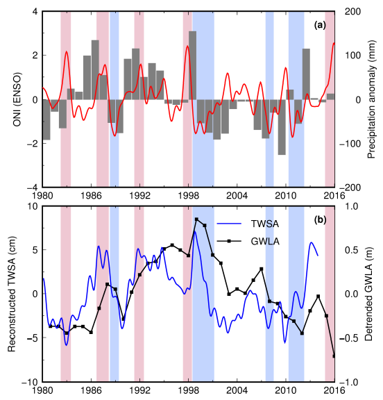
4.4. ENSO’s Effect on Groundwater from a Long-Term Perspective

It is well known that ENSO is an important factor that is influencing the precipitation in some river basins in China, such as the Yellow River basin, the Yangtze River basin, and the Pearl River basin [61,62]. In this study, the significant influence of ENSO on precipitation is also found in the WLRB. In general, precipitation anomalies are positive during the warm phase of ENSO (i.e., El Niño), such as 1987–1988, 1991–1992, and 1997–1998; while, the WLRB experiences the dry conditions during the La Niña events, such as 1988–1989, 1998–2000, 2007–2008, and 2010–2011. Long-term time series of GWLA show a slow decline prior to 1998, followed by a significant rapid decline after that (Figure 3a). The remarkably different behaviors of GWLA before and after 1998 can be attributed to one of the strongest El Niño events on record in 1998 and the following continuous La Niña periods. Detrended time series of GWLA also shows the interannual variability that is related to ENSO (Figure 4b), i.e., GWS increase with El Niño events and decrease with La Niña events.

4.5. Groundwater Recharge and Discharge

According to the water balance, groundwater storage changes in aquifers represent the difference between groundwater recharge and discharge. For the WLRB, to further identify the driver of groundwater depletion, the recharge and discharge status of the aquifers over the WLRB was analyzed. The unconfined aquifer recharge in the WLRB is mainly from the infiltration of precipitation (precipitation infiltration recharge, PIR), which accounts for ~75% of total recharge during normal years, ~57% during dry years, followed by surface water leakage recharge and seepage of irrigation water [29]. Based on the mean atmospheric precipitation infiltration coefficients during the wet (1988–1997) and dry periods (2001–2010), as estimated from Xu [29], the mean PIR decreased significantly from 5.85 km3/yr in the wet years (1984–1998) to 2.35 km3/yr during the dry years (1999–2015). The RESSA also declined rapidly since 1999 in the WLRB [32]. For example, the RESS in the WLRB plain was only 0.13 km3 at the end of 2004, accounting for ~10% of the total design capacity, and most of the reservoirs approached to their dead storage [24]. Therefore, the mean surface water leakage recharge in the WLRB would also decrease due to the reduced surface water storage.
Groundwater discharge is dominated by groundwater exploitation and evaporation from water-table (phreatic) aquifers in the WLRB. These two mechanisms of groundwater discharge account for more than 90% of the total groundwater discharge [24]. As the surface water was largely utilized in the upstream of the WLRB, the source of agricultural irrigation water in the plain region changed from surface water to groundwater since the 1980s [24,63]. Figure 3c shows the annual surface water use and groundwater exploitation in the WLRB since 1998. In the WLRB, mean surface water use was only 0.90 km3/yr from 1998 to 2015, but mean groundwater exploitation was nearly 3.70 km3/yr. The annual groundwater withdrawal for agriculture in the WLRB plain region increased steadily from 0.89 km3 to 1.87 km3 before 1998, but dramatically rose to 2.67 km3 in 1999, and remained at this level after that (Figure 3c). Note that agricultural groundwater exploitation accounts for ~82% of the total groundwater exploitation in the WLRB [29,47]. The increasing large percentage of groundwater use in total water use over the WLRB is consistent with the accelerated groundwater table decline and relatively less precipitation since 1999 (Figure 3a).
Based on the statistics available over the WLRB plain region (Table S1), although the annual precipitation decreased from 426 mm in the 1990s to 323 mm in the 2000s, groundwater irrigation area expanded from 3406 km2 to 5641 km2; meanwhile, crop yield increased from ~3.1 × 10⁶ tons to ~3.8 × 10⁶ tons. Increasing groundwater irrigated area and crop yield, but decreasing precipitation also indicates the serious groundwater overdraft in the WLRB in the 2000s, as consistent with accelerated groundwater level/storage declines after 1998 (Figure 3a and Figure 5b).

5. Conclusions

GWSA in the WLRB was estimated using GRACE and in situ well observations from 2005 to 2015. Significant GWS depletion and interannual variability in the WLRB were detected. GRACE detects a GWS depletion rate of −0.92 ± 0.49 km3/yr, which is equivalent to a total loss of 6.44 km3, during the dry period of 2005–2011. From 2012 to 2015, however, GRACE-derived GWSA shows a prominent inverse V-shape interannual change due to an abnormal precipitation increase in 2012. For the entire 2005–2015 time period, the GWS depletion rate in the WLRB from GRACE is −0.43 ± 0.25 km3/yr. In situ well observations, however, indicate the steady GWS depletion for the entire time period, with a rate of −0.96 ± 0.19 km3/yr from 2005 to 2011, and −0.73 ± 0.15 km3/yr from 2005 to 2015. A remarkable precipitation deficit during the 2000s, associated with La Niña, and continuous groundwater overdraft result in the long-term GWS depletion in the WLRB from 2005 to 2015.
Over a period of almost four decades, long-term interannual TWSA and GWSA in the WLRB are highly correlated with precipitation anomalies, which are driven by ENSO. In general, WLRB receives more precipitation during El Niño and less precipitation during La Niña periods. Annual precipitation is relatively stable during 1980–1997. However, due to the strong 1997–1998 El Niño and the following continuous La Niña, an 11-year drying period after 1998 and the consequent extensive groundwater overexploitation result in significant groundwater depletion in the WLRB. In other words, due to precipitation deficits in the 2000s, groundwater depletion in the WLRB is attributed to both the reduced groundwater recharge from precipitation infiltration and the increasing groundwater discharge due to irrigation.
While GRACE provides a powerful tool to monitor regional GWS variations, there are still large uncertainties in the GRACE-derived GWSA estimates, which mainly result from the GRACE measurement and post-processing errors and the uncertainty in estimated SMSA+SWESA from LSMs. The launch of GRACE Follow-On in early 2018 should extend the TWS observations. The Next Generation Gravity Mission (NGGM) is able to provide higher spatial resolution gravity fields, and will be of great benefit to hydrologic applications [64,65].
In addition, the ongoing development of the new national groundwater monitoring project in China will provide more accurate estimates of GWSA and improved spatial coverage (http.www.mlr.gov.cn/). More space- and ground-based observations with better spatiotemporal resolution and coverage in the near future will enhance our understanding of groundwater changes at the global and regional scales, and guide water resource management for policy makers.

Supplementary Materials

The following are available online at https://www.mdpi.com/2072-4292/10/4/493/s1.

Acknowledgments

This wok was jointly funded by the National Natural Science Foundation of China (41774094, 41431070, 41674084 and 41621091) and the Strategic Priority Research Program of the Chinese Academy of Sciences (XDB23030100). The authors thank Bridget R. Scanlon, Haoming Yan and Peng Peng for their insightful suggestion and discussions, and thank Jin Li, Fan Xie, Liangsheng Shi and Xiaolong Hu for their help in data processing and collection. The authors thank three anonymous reviewers for their helpful comments and suggestions on an earlier version of this paper.

Author Contributions

Yulong Zhong, Wei Feng and Min Zhong designed the experiment; Yulong Zhong conducted the experiments; Yulong Zhong and Wei Feng wrote the manuscript; Zizhan Zhang revised the manuscript; Yingchun Shen and Dingcheng Wu collected and analyzed parts of the data; Min Zhong and Wei Feng provided the financial support and rationalized the logic of the manuscript.

Conflicts of Interest

The authors declare no conflict of interest.

References

  1. Konikow, L.F.; Kendy, E. Groundwater depletion: A global problem. Hydrogeol. J. 2005, 13, 317–320. [Google Scholar] [CrossRef]
  2. Rodell, M.; Velicogna, I.; Famiglietti, J.S. Satellite-based estimates of groundwater depletion in India. Nature 2009, 460, 999–1002. [Google Scholar] [CrossRef] [PubMed]
  3. Scanlon, B.R.; Longuevergne, L.; Long, D. Ground referencing GRACE satellite estimates of groundwater storage changes in the California Central Valley, USA. Water Resour. Res. 2012, 48, 04520. [Google Scholar] [CrossRef]
  4. Tourian, M.J.; Elmi, O.; Chen, Q.; Devaraju, B.; Roohi, S.; Sneeuw, N. A spaceborne multisensor approach to monitor the desiccation of Lake Urmia in Iran. Remote Sens. Environ. 2015, 156, 349–360. [Google Scholar] [CrossRef]
  5. Liu, C.M.; Yu, J.J.; Eloise, K. Groundwater exploitation and its impact on the environment in the North China Plain. Water Int. 2001, 26, 265–272. [Google Scholar]
  6. Strassberg, G.; Scanlon, B.R.; Chambers, D. Evaluation of groundwater storage monitoring with the GRACE satellite: Case study of the High Plains aquifer, central United States. Water Resour. Res. 2009, 45, W05410. [Google Scholar] [CrossRef]
  7. Sun, A.Y.; Green, R.; Rodell, M.; Swenson, S. Inferring aquifer storage parameters using satellite and in situ measurements: Estimation under uncertainty. Geophys. Res. Lett. 2010, 37, L10401. [Google Scholar] [CrossRef]
  8. Doll, P.; Hoffmann-Dobrev, H.; Portmann, F.T.; Siebert, S.; Eicker, A.; Rodell, M.; Strassberg, G.; Scanlon, B.R. Impact of water withdrawals from groundwater and surface water on continental water storage variations. J. Geodyn. 2012, 59–60, 143–156. [Google Scholar] [CrossRef]
  9. Tapley, B.D.; Bettadpur, S.; Ries, J.C.; Thompson, P.F.; Watkins, M.M. GRACE measurements of mass variability in the Earth system. Science 2004, 305, 503–505. [Google Scholar] [CrossRef] [PubMed]
  10. Wahr, J.; Swenson, S.; Zlotnicki, V.; Velicogna, I. Time-variable gravity from GRACE: First results. Geophys. Res. Lett. 2004, 31, L11501. [Google Scholar] [CrossRef]
  11. Long, D.; Pan, Y.; Zhou, J.; Chen, Y.; Hou, X.Y.; Hong, Y.; Scanlon, B.R.; Longueyergne, L. Global analysis of spatiotemporal variability in merged total water storage changes using multiple GRACE products and global hydrological models. Remote Sens. Environ. 2017, 192, 198–216. [Google Scholar] [CrossRef]
  12. Rodell, M.; Chen, J.L.; Kato, H.; Famiglietti, J.S.; Nigro, J.; Wilson, C.R. Estimating groundwater storage changes in the Mississippi River basin (USA) using GRACE. Hydrogeol. J. 2007, 15, 159–166. [Google Scholar] [CrossRef]
  13. Strassberg, G.; Scanlon, B.R.; Rodell, M. Comparison of seasonal terrestrial water storage variations from GRACE with groundwater-level measurements from the High Plains Aquifer (USA). Geophys. Res. Lett. 2007, 34. [Google Scholar] [CrossRef]
  14. Long, D.; Chen, X.; Scanlon, B.R.; Wada, Y.; Hong, Y.; Singh, V.P.; Chen, Y.; Wang, C.; Han, Z.; Yang, W. Have GRACE satellites overestimated groundwater depletion in the Northwest India Aquifer? Sci. Rep. 2016, 6, 24398. [Google Scholar] [CrossRef] [PubMed] [Green Version]
  15. Chen, J.L.; Li, J.; Zhang, Z.Z.; Ni, S.N. Long-term groundwater variations in Northwest India from satellite gravity measurements. Glob. Planet. Chang. 2014, 116, 130–138. [Google Scholar] [CrossRef]
  16. Tiwari, V.M.; Wahr, J.; Swenson, S. Dwindling groundwater resources in northern India, from satellite gravity observations. Geophys. Res. Lett. 2009, 36, L18401. [Google Scholar] [CrossRef]
  17. Bhanja, S.N.; Mukherjee, A.; Saha, D.; Velicogna, I.; Famiglietti, J.S. Validation of GRACE based groundwater storage anomaly using in-situ groundwater level measurements in India. J. Hydrol. 2016, 543, 729–738. [Google Scholar] [CrossRef]
  18. Famiglietti, J.S.; Lo, M.; Ho, S.L.; Bethune, J.; Anderson, K.J.; Syed, T.H.; Swenson, S.C.; de Linage, C.R.; Rodell, M. Satellites measure recent rates of groundwater depletion in California’s Central Valley. Geophys. Res. Lett. 2011, 38, L03403. [Google Scholar] [CrossRef]
  19. Scanlon, B.R.; Faunt, C.C.; Longuevergne, L.; Reedy, R.C.; Alley, W.M.; McGuire, V.L.; McMahon, P.B. Groundwater depletion and sustainability of irrigation in the US High Plains and Central Valley. Proc. Natl. Acad. Sci. USA 2012, 109, 9320–9325. [Google Scholar] [CrossRef] [PubMed] [Green Version]
  20. Feng, W.; Zhong, M.; Lemoine, J.M.; Biancale, R.; Hsu, H.T.; Xia, J. Evaluation of groundwater depletion in North China using the Gravity Recovery and Climate Experiment (GRACE) data and ground-based measurements. Water Resour. Res. 2013, 49, 2110–2118. [Google Scholar] [CrossRef]
  21. Huang, Z.Y.; Pan, Y.; Gong, H.L.; Yeh, P.J.F.; Li, X.J.; Zhou, D.M.; Zhao, W.J. Subregional-scale groundwater depletion detected by GRACE for both shallow and deep aquifers in North China Plain. Geophys. Res. Lett. 2015, 42, 1791–1799. [Google Scholar] [CrossRef]
  22. Moiwo, J.P.; Tao, F.L.; Lu, W.X. Analysis of satellite-based and in situ hydro-climatic data depicts water storage depletion in North China Region. Hydrol. Process. 2013, 27, 1011–1020. [Google Scholar] [CrossRef]
  23. Joodaki, G.; Wahr, J.; Swenson, S. Estimating the human contribution to groundwater depletion in the Middle East, from GRACE data, land surface models, and well observations. Water Resour. Res. 2014, 50, 2679–2692. [Google Scholar] [CrossRef]
  24. Li, Z.; Yu, M.W.; Zhang, L.L.; Liu, B.S.; Long, W.H.; Wang, A.S.; Feng, B.A.; Huo, G.L. Investigation and Assessment of Groundwater Resources and Their Environmental Issues in the West Liaohe Plain; Geological Publishing House: Beijing, China, 2009; p. 313. [Google Scholar]
  25. Liang, H.Y. Changes of Light, Heat, Water Resources and Effect on Corn Potential Productivity in Xiliao River Plain; Inner Mongolia University for Nationalities: Tongliao, China, 2010. [Google Scholar]
  26. Gao, S.; Tang, Y.; Tang, K.W. Groundwater vulnerability assessment in Tongliao Plain, Inner Mongolia. J. China Inst. Water Resour. Hydrop. Res. 2015, 13, 10. [Google Scholar]
  27. Songliao Water Resources Commission (SLWRC). Songliao Basin Water Resources Bulletin; Songliao Water Resources Commission: Changchun, China, 2013.
  28. Inner Mongolia Water Resources Protection and Project Group (IMWRPPG). Inner Mongolia Songliao Basin Groundwater Protection and Project; Hydrological Bur. of Inner Mongolia; Inner Mongolia Water Resources Protection and Project Group: Hohhot, China, 2014. [Google Scholar]
  29. Xu, K. Study on Water Cycle Regulation in West Liao River Basin and Ecosystem Stability of West Liao River Plain. D; China Institute of Water Resources and Hydropower Research: Beijing, China, 2013. [Google Scholar]
  30. Zhang, Q.; Singh, V.P.; Sun, P.; Chen, X.; Zhang, Z.X.; Li, J.F. Precipitation and streamflow changes in China: Changing patterns, causes and implications. J. Hydrol. 2011, 410, 204–216. [Google Scholar] [CrossRef]
  31. Chen, Z.Y. Research on the Response of Groundwater Depth Change and the Vegetation Ecosystem in the West Liao River Plain Based on RS/GIS D; Jilin University: Changchun, China, 2012. [Google Scholar]
  32. Hydrological Bureau of Inner Mongolia (HBIM). Inner Mongolia Water Resources Bulletin; Department of Water Resources of Inner Mongolia: Hohhot, China, 2013.
  33. Yang, H.S.; Liu, J.; Liang, H.Y. Change characteristics of climate and water resources in West Liaohe River Plain. Chin. J. Appl. Ecol. 2009, 20, 84–90. [Google Scholar]
  34. Zhu, T.T.; Hai, J.Y. Brief discussion about water resource in Tongliao. J. Inner Mon. Univ. Natl. 2008, 14, 97–98. [Google Scholar]
  35. Long, W.H.; Chen, H.H.; Li, Z.; Pan, H.J. Evaluation of the groundwater intrinsic vulnerability in West Liaohe Plain, Inner Mongolia, China. Geol. Bull. China 2010, 29, 598–602. [Google Scholar]
  36. Zhao, Z.Z.; Lin, A.W.; Feng, J.D.; Yang, Q.; Zou, L. Analysis of water resources in Horqin Sandy land using multisource data from 2003 to 2010. Sustainability 2016, 8, 374. [Google Scholar] [CrossRef]
  37. Wu, K.; Wang, X.L.; Wang, G.X.; Wu, Y.X. Spatial-temporal variation of precipitation in West Liao River Basin during 1961–2014. S. N. Water Transf. Water Sci. Technol. 2017, 15, 22–28. [Google Scholar]
  38. Save, H.; Bettadpur, S.; Tapley, B.D. High-resolution CSR GRACE RL05 mascons. J. Geophys. Res. Solid Earth 2016, 121, 7547–7569. [Google Scholar] [CrossRef]
  39. Scanlon, B.R.; Zhang, Z.Z.; Save, H.; Wiese, D.N.; Landerer, F.W.; Long, D.; Longuevergne, L.; Chen, J.L. Global evaluation of new GRACE mascon products for hydrologic applications. Water Resour. Res. 2016, 52, 9412–9429. [Google Scholar] [CrossRef]
  40. Ek, M.; Mitchell, K.; Lin, Y.; Rogers, E.; Grunmann, P.; Koren, V.; Gayno, G.; Tarpley, J. Implementation of Noah land surface model advances in the National Centers for Environmental Prediction operational mesoscale Eta model. J. Geophys. Res. Atmos. 2003, 108, 8851. [Google Scholar] [CrossRef]
  41. Dai, Y.J.; Zeng, X.B.; Dickinson, R.E.; Baker, I.; Bonan, G.B.; Bosilovich, M.G.; Denning, A.S.; Dirmeyer, P.A.; Houser, P.R.; Niu, G.Y.; et al. The Common Land Model. Bull. Am. Meteorol. Soc. 2003, 84, 1013–1023. [Google Scholar] [CrossRef]
  42. Koster, R.D.; Suarez, M.J. Modeling the land surface boundary in climate models as a composite of independent vegetation stands. J. Geophys. Res. Atmos. 1992, 97, 2697–2715. [Google Scholar] [CrossRef]
  43. Liang, X.; Lettenmaier, D.P.; Wood, E.F.; Burges, S.J. A simple hydrologically based model of land surface water and energy fluxes for general circulation models. J. Geophys. Res. Atmos. 1994, 99, 14415–14428. [Google Scholar] [CrossRef]
  44. Rodell, M.; Houser, P.R.; Jambor, U.; Gottschalck, J.; Mitchell, K.; Meng, C.J.; Arsenault, K.; Cosgrove, B.; Radakovich, J.; Bosilovich, M.; et al. The global land data assimilation system. Bull. Am. Meteorol. Soc. 2004, 85, 381–394. [Google Scholar] [CrossRef]
  45. China Institute of Geological Environment Monitoring (CIGEM). China Geological Environment Monitoring: Groundwater Yearbook; China Land Press: Beijing, China, 2013. [Google Scholar]
  46. Xiao, R.Y.; He, X.F.; Zhang, Y.L.; Ferreira, V.G.; Chang, L. Monitoring groundwater variations from satellite gravimetry and hydrological models: A comparison with in-situ measurements in the mid-Atlantic region of the United States. Remote Sens. 2015, 7, 686–703. [Google Scholar] [CrossRef]
  47. Songliao Water Resources Commission (SLWRC). Songliao Basin Groundwater Bulletin; Songliao Water Resources Commission: Changchun, China, 2013.
  48. Humphrey, V.; Gudmundsson, L.; Seneviratne, S.I. A global reconstruction of climate-driven subdecadal water storage variability. Geophys. Res. Lett. 2017, 44, 2300–2309. [Google Scholar] [CrossRef]
  49. Humphrey, V.; Gudmundsson, L.; Seneviratne, S.I. Assessing Global Water Storage Variability from GRACE: Trends, Seasonal Cycle, Subseasonal Anomalies and Extremes. Surv. Geophys. 2016, 37, 357–395. [Google Scholar] [CrossRef] [PubMed]
  50. Yi, S.; Sun, W.K.; Feng, W.; Chen, J.L. Anthropogenic and climate-driven water depletion in Asia. Geophys. Res. Lett. 2016, 43, 9061–9069. [Google Scholar] [CrossRef]
  51. Landerer, F.W.; Swenson, S.C. Accuracy of scaled GRACE terrestrial water storage estimates. Water Resour. Res. 2012, 48, W04531. [Google Scholar] [CrossRef]
  52. Gao, Y.B.; Nie, Q.H.; He, X.D.; Chang, X.L.; He, H.L. Tactic phase and potential of grass plantation in Horqin sand land Taking Tongliao city of inner mongolia autonomous region as an example. J. Des. Res. 2003, 23, 242–245. [Google Scholar]
  53. Vondrák, J. Problem of smoothing observational data II. Bull. Astron. Inst. Czech. 1977, 28, 84. [Google Scholar]
  54. Zheng, D.W.; Zhong, P.; Ding, X.L.; Chen, W. Filtering GPS time-series using a Vondrak filter and cross-validation. J. Geod. 2005, 79, 363–369. [Google Scholar] [CrossRef]
  55. Yu, C.J. Dynamic Simulation Evaluation about Water Resource System and Optimal Allocation Model of Macro-Economy Water Resource in Tong Liao City; Inner Mongolia Agricultural University: Hohhot, China, 2004. [Google Scholar]
  56. Longuevergne, L.; Wilson, C.R.; Scanlon, B.R.; Cretaux, J.F. GRACE water storage estimates for the Middle East and other regions with significant reservoir and lake storage. Hydrol. Earth Syst. Sci. 2013, 17, 4817–4830. [Google Scholar] [CrossRef] [Green Version]
  57. Yi, S.; Song, C.Q.; Wang, Q.Y.; Wang, L.S.; Heki, K.; Sun, W.K. The potential of GRACE gravimetry to detect the heavy rainfall-induced impoundment of a small reservoir in the upper Yellow River. Water Resour. Res. 2017, 53, 6562–6578. [Google Scholar] [CrossRef]
  58. Wiese, D.N.; Landerer, F.W.; Watkins, M.M. Quantifying and reducing leakage errors in the JPL RL05M GRACE Mascon solution. Water Resour. Res. 2016, 52, 7490–7502. [Google Scholar] [CrossRef]
  59. Luthcke, S.B.; Sabaka, T.J.; Loomis, B.D.; Arendt, A.A.; McCarthy, J.J.; Camp, J. Antarctica, Greenland and Gulf of Alaska land-ice evolution from an iterated GRACE global mascon solution. J. Glaciol. 2013, 59, 613–631. [Google Scholar] [CrossRef]
  60. Kusche, J.; Schmidt, R.; Petrovic, S.; Rietbroek, R. Decorrelated GRACE time-variable gravity solutions by GFZ, and their validation using a hydrological model. J. Geodesy 2009, 83, 903–913. [Google Scholar] [CrossRef]
  61. Ouyang, R.; Liu, W.; Fu, G.; Liu, C.; Hu, L.; Wang, H. Linkages between ENSO/PDO signals and precipitation, streamflow in China during the last 100 years. Hydrol. Earth Syst. Sci. 2014, 18, 3651–3661. [Google Scholar] [CrossRef]
  62. Zhang, Q.; Xu, C.Y.; Jiang, T.; Wu, Y.J. Possible influence of ENSO on annual maximum streamflow of the Yangtze River, China. J. Hydrol. 2007, 333, 265–274. [Google Scholar] [CrossRef]
  63. Yang, X.L.; Ren, L.L.; Jiang, S.H.; Yuan, S.S.; Shi, L. Analysis of trend and influencing factors of runoff variation in headwater basin of West Liaohe River. J. Hohai Univ. 2012, 40, 37–41. [Google Scholar]
  64. Pail, R.; Bingham, R.; Braitenberg, C.; Dobslaw, H.; Eicker, A.; Güntner, A.; Horwath, M.; Ivins, E.; Longuevergne, L.; Panet, I. Science and user needs for observing global mass transport to understand global change and to benefit society. Surv. Geophys. 2015, 36, 743–772. [Google Scholar] [CrossRef]
  65. Panet, I.; Flury, J.; Biancale, R.; Gruber, T.; Johannessen, J.; van den Broeke, M.; van Dam, T.; Gegout, P.; Hughes, C.; Ramillien, G. Earth system mass transport mission (e.motion): A concept for future earth gravity field measurements from space. Surv. Geophys. 2013, 34, 141–163. [Google Scholar] [CrossRef] [Green Version]
Figure 1. Map of the West Liaohe Basin (WLRB, black boundary). The main rivers are shown in blue. The observation wells are shown as circles. The colors represent the groundwater level trends from 2005 to 2011. The insert map shows the location of the WLRB (red shade) in China.
Remotesensing 10 00493 g001
Figure 2. (a) Time series of terrestrial water storage anomalies (TWSA) estimated from Gravity Recovery and Climate Experiment (GRACE) and soil moisture storage anomalies (SMSA)+snow water equivalent storage anomalies (SWESA) derived from Global Land Data Assimilation System (GLDAS) land surface models (LSMs), with seasonal cycles removed. The blue and orange shadows represent the uncertainties in TWSA and SMSA+SWESA; (b) Time series of GWSA from in situ well measurements and from GRACE and GLDAS LSMs, with seasonal cycles removed. The shadows show the uncertainties in GWSA; (c) Annual GWS variations in volume derived from GRACE, in situ well measurements, and Water Resources Bulletin (WRB). The gray bars show annual precipitation anomalies relative to the average of annual precipitation during 1980–2015.
Remotesensing 10 00493 g002
Figure 3. (a) Time series of mean groundwater table depth in the WLRB from 1980 to 2015. The blue and red dash lines show the groundwater level trends for 1980–1998 and 1999–2015, respectively; (b) Time series of annual groundwater exploitation amount due to agricultural irrigation from 1987 to 2010 in the WLRB plain based on the statistics from Yu [55] and groundwater bulletins from the SLWRC [47]; and, (c) Time series of annual consumption of groundwater (red line) and surface water (black line) in the WLRB from 1998 to 2015.
Remotesensing 10 00493 g003
Figure 4. (a) Annual precipitation anomalies relative to mean precipitation of 1980–2015 in the WLRB. The red line shows the Oceanic Niño Index (ONI) with a Vondrak filter applied to exclude the high-frequency signal. The blue shadows show the warm El Niño-Southern Oscillation (ENSO) phase (El Niño) and pink shadows represent the cold ENSO phase (La Niña); (b) The blue line shows the time series of reconstructed TWSA from 1980 to 2013, with a Vondrak filter applied. The black line with squares shows mean groundwater level anomalies in the WLRB, with the secular trend removed.
Remotesensing 10 00493 g004
Figure 5. (a) Time series of GWF from 1980 to 2015 and regression-modeled GWF for 1980–1998 and 1998–2015 for the WLRB; (b) Time series of GWSA and reconstructed GWSA from 1980 to 2015 for the WLRB.
Remotesensing 10 00493 g005
Table 1. Summary of the datasets used in this study.
TypeData NameData Version/SourceSpatial and Temporal Resolution, Ttime PeriodData Access
SatelliteTWSACSR Mascons1° × 1°, monthly, 2005–2015http://www2.csr.utexas.edu/grace/RL05_mascons.html
ModelsSMSA+SWESAGLDAS-1 LSMs1° × 1°, monthly, 2005–2015http://mirador.gsfc.nasa.gov/
In situGWSACIGEM+HBIM122 wells, monthly, 2005–2015Groundwater yearbook and Hydrological Bureau of Inner Mongolia
GWLA Region mean, annual, 1980–2015http://116.113.33.52:8989/ and Xu [29]
RESSA Region sum, annual, 1997–2015http://116.113.33.52:8989/
PrecipitationCMDC0.5° × 0.5°, monthly, 1961–2015http://data.cma.cn/
0.5° × 0.5°, daily, 1961–2013http://data.cma.cn/
Climate indicesONI Time series, monthly, 1980–2015http://origin.cpc.ncep.noaa.gov/products/analysis_monitoring/ensostuff/ONI_v5.php
Table 2. GWS rates in the WLRB estimated from different GRACE solutions. Center for Space Research (CSR)-M represents the CSR Mascons used in this study [38]; i.e., JPL-M.dsf represents the Jet Propulsion Laboratory (JPL) Global Mascons [58] with grid scaling factors applied; GSFC-M represents the Goddard Space Flight Center (GSFC) Global Mascons [59]; CSRT-GSH represents GRCTellus Land data [51]; while, CSR-DDK3 represents CSR spherical harmonic solutions with DDK3 filtered [60]. The uncertainties were given as the standard deviations, which means that the error bounds represent the 68% confidence interval.
GRACE SolutionsRate (km3/yr)Rate (km3/yr)
January 2005–December 2011January 2005–December 2015
CSR-M−0.92 ± 0.49−0.43 ± 0.26
JPL-M.dsf−1.54 ± 0.42−0.45 ± 0.21
GSFC-M−1.47 ± 0.46−0.62 ± 0.23
CSRT-GSH−0.84 ± 0.47−0.51 ± 0.24
CSR-DDK3−1.67 ± 0.65−0.65 ± 0.33

