Article

Estimating Peatland Water Table Depth and Net Ecosystem Exchange: A Comparison between Satellite and Airborne Imagery

1
Applied Remote Sensing Laboratory, Department of Geography, McGill University, Montréal, QC H3A 0B9, Canada
2
Flight Research Laboratory, National Research Council of Canada, Ottawa, ON K1A-0R6, Canada
3
Geography and Environmental Studies, Carleton University, Ottawa, ON K1S 5B6, Canada
*
Author to whom correspondence should be addressed.
Remote Sens. 2018, 10(5), 687; https://doi.org/10.3390/rs10050687
Submission received: 23 February 2018 / Revised: 24 April 2018 / Accepted: 24 April 2018 / Published: 29 April 2018
(This article belongs to the Special Issue Remote Sensing of Peatlands)

Abstract

:
Peatlands play a fundamental role in climate regulation through their long-term accumulation of atmospheric carbon. Despite their resilience, peatlands are vulnerable to climate change. Remote sensing offers the opportunity to better understand these ecosystems at large spatial scales through time. In this study, we estimated water table depth from a 6-year time sequence of airborne shortwave infrared (SWIR) hyperspectral imagery. We found that the narrowband index NDWI1240 is a strong predictor of water table position. However, we illustrate the importance of considering peatland anisotropy on SWIR imagery from the summer months when the vascular plants are in full foliage, as not all illumination conditions are suitable for retrieving water table position. We also model net ecosystem exchange (NEE) from 10 years of Landsat TM5 imagery and from 4 years of Landsat OLI 8 imagery. Our results show the transferability of the model between imagery from sensors with similar spectral and radiometric properties such as Landsat 8 and Sentinel-2. NEE modeled from airborne hyperspectral imagery more closely correlated to eddy covariance tower measurements than did models based on satellite images. With fine spectral, spatial and radiometric resolutions, new generation satellite imagery and airborne hyperspectral imagery allow for monitoring the response of peatlands to both allogenic and autogenic factors.

Graphical Abstract

1. Introduction

Northern peatlands have played a significant role in carbon (C) accumulation for millennia [1]. Because of their large extent in northern regions (e.g., 12% of Canada, or 1 million km2) [2,3,4], it is important to evaluate their potential response to climate change [5,6]. Remote sensing studies of peatlands from both hyperspectral airborne and multispectral satellite sensors have shown potential in providing fundamental information about vegetation (e.g., leaf area index) and hydrology, especially with respect to the spatial patterns and temporal trends of these characteristics at large spatial scales (>100 ha) (e.g., [7,8,9,10,11]). The advantage of airborne hyperspectral imagery in peatland research is that it can be collected at a fine spatial resolution (≤1 m) to carry out detailed mapping and modeling studies (e.g., [8,9,12]). However, due to the inaccessible nature of many peatlands [3] and the elevated cost of such data acquisition, especially for isolated northern peatlands, satellite imagery might be the most feasible long-term monitoring solution for these ecosystems. A novel aspect of peatland research using remotely sensed data is the integration of airborne hyperspectral imagery with multispectral satellite data for ecosystem modeling (e.g., hydrology, biogeochemistry).
Optical imagery in the VNIR (visible-near infrared) and SWIR (shortwave infrared) ranges (400–2500 nm) has been used to determine spectral differences between mosses and vascular plants in peatlands [13]. Spectral indices incorporating both narrow and broadband sensors (e.g., [14]) successfully assessed the relationship between surface moisture and water table position experimentally and at small spatial scales [8,15]. However, remote sensing studies at the ecosystem level are still needed to evaluate the full potential of such imagery, especially for peatlands where in situ data are available. Furthermore, a more thorough understanding of the effects of illumination and viewing geometries are needed for studies considering seasonal changes.
The difference between the carbon dioxide uptake through gross primary production (GPP) and ecosystem respiration represents the net ecosystem exchange (NEE) [16]. In situ measurement of NEE via approaches such as flux chambers can be utilized to assess responses to diverse variables, including nutrient inputs (e.g., [17]) and manipulations of water content [18]. Eddy covariance towers are also commonly used in the assessment of NEE in peatland ecosystems, with the advantage that these provide a larger footprint than chambers and can provide near-continuous long-term data [19,20]. For large-scale studies, MODIS-derived products have been used to assess NEE [21,22], however, the large spatial resolution (e.g., 0.5–1 km) is inadequate to capture the small-scale heterogeneity of peatlands, along with other known limitations for peatlands such as the errors in the vapor pressure deficit determined from land cover (for GPP estimation) [23,24]. More recently, the potential of Landsat 7 ETM+ data (30 m resolution) was shown for determining peatland classes with high accuracy [23], from which to estimate the C balance. Given the long history of the Landsat program, a less explored aspect is the development of C models (e.g., NEE) taking advantage of these multitemporal data. In addition, new satellites such as Sentinel-2 provide additional opportunities to evaluate Landsat products at finer spatial scales (e.g., 10–20 m spatial resolution), which may better capture the spatial heterogeneity of these ecosystems.
Biogeochemical processes such as gas exchange (e.g., CO2, CH4) and C accumulation in northern peatlands are closely related to the water table position [25,26,27]. Given a lowering of the water table, an increase in CO2 loss is expected [25]. For example, the interannual variability of C exchange at the Mer Bleue peatland indicated that this ecosystem reduced its CO2 sink capacity during summertime drought events [20]. However, there is high variability in CO2 exchange across peatland sites and seasonally within sites [16]. Spatial variability of the vegetation composition [28] and other variables, such as temperature [29,30], also impact the overall C budget of these ecosystems. Therefore, ongoing characterization of the spatial and temporal variability of the water table position and CO2 uptake in peatlands is necessary.
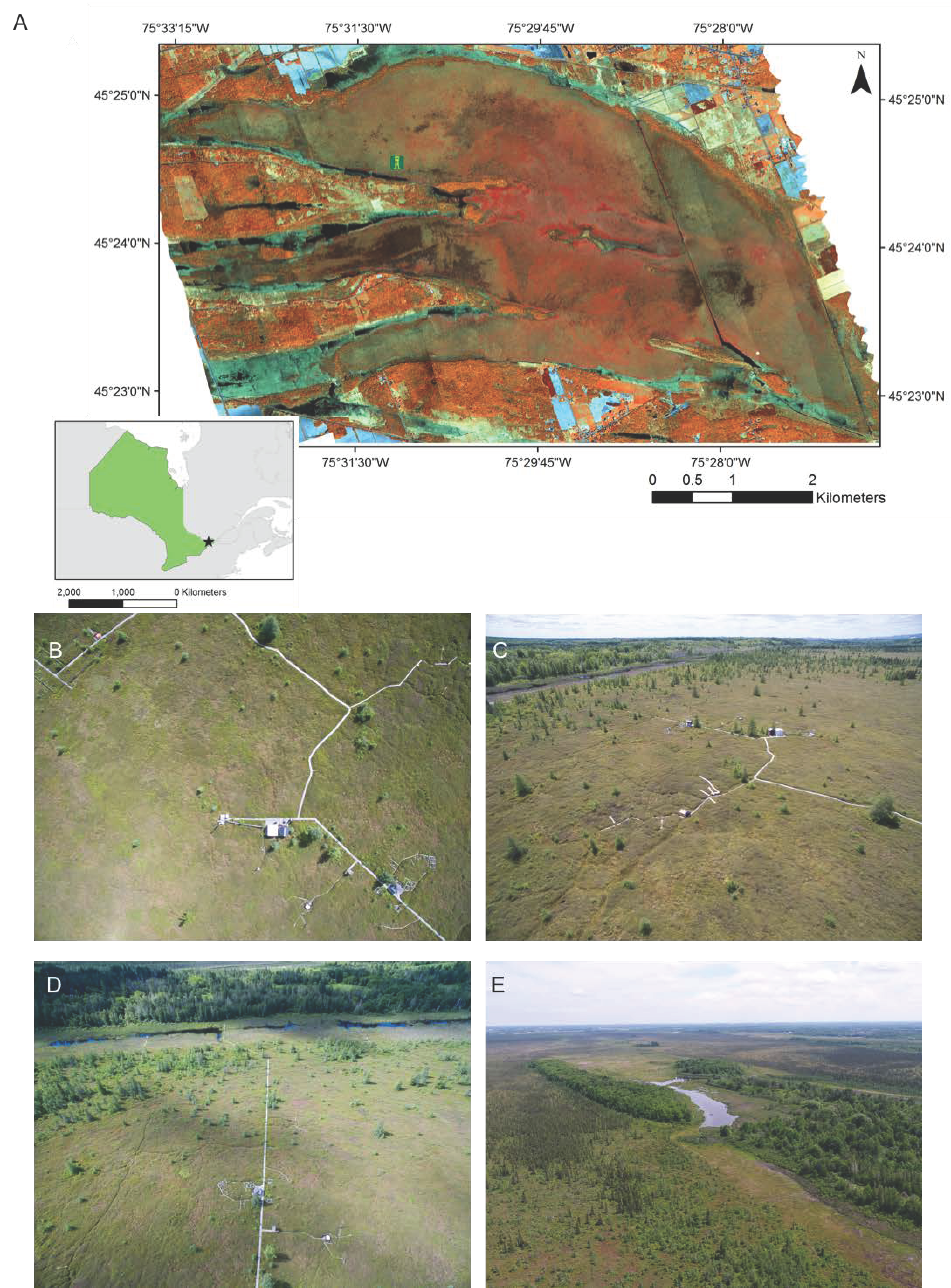
In this study, we addressed two distinct but complementary objectives for estimating water table depth and NEE at the Mer Bleue Conservation Area using remotely sensed data. The first objective was to assess the relationship between a surface moisture index derived from SWIR hyperspectral imagery and water table depth. We hypothesized that changes in vegetation surface moisture throughout the growing season at Mer Bleue are closely related to water table depth [8]; therefore, such an index could be used as a proxy. The second objective was to develop and test a NEE model based on a modified water index (MWI) calculated from multitemporal Landsat TM5 and Landsat 8 OLI data. As vegetation moisture content and phenology are closely related to CO2 uptake in peatlands [8], we predicted that the model could serve as a good estimator of NEE at large spatial scales. We applied the resultant NEE models to multitemporal Sentinel-2A and airborne hyperspectral VNIR imagery to determine spatial and temporal trends during the 2016 growing season and compare the results with observed NEE from an eddy covariance tower. This study builds upon results by [31], mapping near surface water content in hollows and light-saturated gross photosynthesis for hummocks in the same peatland.

2. Materials and Methods

2.1. Study Area

The ~8500 year-old Mer Bleue ombrotrophic bog [20] is located centrally within the 35 km2 Mer Bleue Conservation Area east of Ottawa, ON, Canada (Figure 1a). Mer Bleue is recognized as a ‘Wetland of International Importance’ under the Ramsar Convention on Wetlands, a ‘Provincially Significant Wetland, and a Provincially Significant Life and Earth Science Area of Natural and Scientific Interest’. Oxygen isotope records from the peat indicate the site followed a paleotemperature trend similar to that of other sites in the Northern Hemisphere with well-known cool events such as the Little Ice Age and the 1815 eruption of the Tambora volcano visible in the records [32].
The bog is acidic and nutrient-poor, receiving incoming water and nutrients from precipitation and deposition. Along its long axis it is dissected by two longitudinal sections of fluvial sand and gravel separating three distinct “fingers” at the western end of the peatland [20] (Figure 1a). The climate is cool continental temperate with a 30-year (1971–2000) mean annual air temperature of 6.0 °C. The mean annual precipitation is 943 mm, of which 235 mm falls as snow, generally between December and March [33]. The bog is slightly domed, with a peat depth increasing from 0.3 m along the edge to greater than 5 m across most of the area. Beaver ponds around the margins are inundated year-round and have extensive cattail (Typha angustifolia) and floating Sphagnum moss coverage [20,33]. Mer Bleue has a hummock-hollow-lawn microtopography over the majority of its area with a mean relief between hummocks and hollows of less than 30 cm [34,35]. The variable water table is generally below the surface of the hollows throughout the growing season [20]. In addition, there are treed bog and poor fen sections, and relatively dense mixed forest [11]. While the vegetation composition has been extensively described (see [11,36]), the main vascular plant species found in the bog are evergreen and deciduous shrubs (Chamaedaphne calyculata, Rhododendron groenlandicum, Kalmia angustifolia, Vaccinium myrtilloides), sedges (Eriophorum vaginatum), and a few trees Picea mariana, Betula populifolia, and Larix laricina. The main Sphagnum mosses in the bog are S. capillifolium and S. magellanicum. While the mosses form the ground layer of the bog and are exposed in hollows, vascular plants comprise the upper plant canopy of the hummocks [37]. Conservatively, hummocks account for 51.2%, hollows for 12.7%, and trees for 33.6% of the entire bog’s surface area (excluding the surrounding mineral soils), with other classes such as open water comprising the remaining 2.4% [31]. As in [31], we focused our analysis on a 19 km2 section of Mer Bleue which is solely composed of the peatland without the surrounding treed areas on mineral soil (Figure 1).

2.2. Airborne Hyperspectral Imagery (HSI)

The airborne HSI was acquired over a period of 5 years from 2011–2016. Two HSI sensors that record complementary regions of the electromagnetic spectrum were used: a Compact Airborne Spectrographic Imager 1500 (CASI-1500, hereafter referred to as CASI) and a Shortwave Airborne Spectrographic Imager (SASI-644, hereafter referred to as SASI) (ITRES Ltd., Calgary, AB, Canada). The programable CASI samples a maximum of 288 spectral channels between 375 nm and 1054 nm, with 1493–1498 across track pixels, and a field of view of 39.9°. The SASI samples 160 spectral channels from 883 nm to 2523 nm, with 640 across track pixels, and a field of view of 39.7° [31,38]. In this study, we used 18 flight-lines from the SASI (2011–2016) for the estimation of the water table position (Table 1). NEE estimation was derived from 4 individual flight lines and 4 full bog mosaics from the CASI (for 2016) (Table 2). The mosaics are comprised of 12 flight lines with a 20% overlap. The higher temporal frequency of HSI acquisition in 2015 and 2016 is due to Mer Bleue being designated a validation site for Sentinel-2 and Landsat 8 OLI satellite data products [39].
As described in [31], the individual HSI flight lines were spectroradiometrically calibrated to units of spectral radiance (µW cm−2 sr−1 nm−1). The preprocessing steps to calibrate the imagery from raw digital number to radiance were performed using software modules developed by the sensors’ manufacturer [40]. The subsequent geocorrection process was performed using results from a bundling calibration designed to relate the inertial measurement unit (C-MIGITS II) (IMU—a combined GPS and inertial navigation system) to the sensor geometry. The preprocessing modules include an image-based assessment and correction of the spectral alignment and a removal of signal offsets inherent in the recorded digital pixel values (i.e., electronic offset, dark current, frame shift smear, scattered light, and, for the CASI, only a second-order diffracted light correction) [38,39,40,41]. Further preprocessing steps included spectroradiometric calibration, spectral resampling to remove the laboratory-identified spectral smile, and geocorrection. A single CASI flight line (23 September 2016) was not geocorrectable due to an error in the IMU data. For the four CASI mosaics, we used a “minimize view zenith angle” option to select which of the duplicate pixels located in the overlap between adjacent flight lines are applied in the resulting mosaic imagery. During geocorrection, all HSI flight lines were resampled to 1 m pixel size.
Mission planning attempted to acquire the HSI lines coincident with the Sentinel-2A satellite overpasses in 2015 and 2016, and utilized a planned ground-track designed to optimize the alignment with respect to the solar azimuth angle (SAA) to minimize cross-track illumination effects. Weather was taken into consideration to avoid acquisition during cloudy conditions. All lines were acquired within 2.5 h of solar noon. For the individual SASI and CASI flight lines, the atmospheric correction was performed with the FLAASH module in the ENVI 5.4.1. For the CASI mosaics, atmospheric correction was applied to the individual flight lines using ATCOR4 4.7.0 for flat terrain prior to the application of a cross-track illumination correction and image mosaicking [31].

2.3. Satellite Imagery

2.3.1. Landsat TM5 Imagery

Atmospherically corrected surface reflectance Landsat TM5 (1999–2011) and Landsat 8 OLI (2013–2016) (both Collection 1, Tier 1) data were used to derive models of yearly cumulative NEE (Table A1). A query of the USGS archives through Google Earth Engine [42] yielded a catalog of 488 and 172 scenes of Mer Bleue, respectively, for the eddy covariance tower footprint area considered here (55,800 m2). Only snow- and cloud-free scenes for the study area were retained for the months spanning from April to November. The temporal frequency of the scenes in the collection was uneven between years, ranging from 5 to over 20. Therefore, in order for a year to be included in the models (Section 2.5.2), multiple scenes were required from all three seasons (i.e., spring (leaf off): prior to vascular vegetation green-up; summer: full foliage; and fall: senescent vascular vegetation). With these criteria, 175 scenes for TM5 and 63 scenes for OLI8 were retained (Table 3).

2.3.2. Sentinel-2 Imagery

The NEE models (Section 2.5.2) were applied to nine Sentinel-2A scenes (cloud- and snow-free over the study area) acquired in 2016 (Table 4). The scenes were retrieved from the USGS Earth Explorer as Level 1C, orthorectified top of the atmosphere (TOA) reflectance [43,44]. In order to produce Level 2A surface reflectance (i.e., bottom of atmosphere (BOA) product), the scenes were processed using Sen2cor 2.2.1 [45]. The reflectance images were created at 20 m spatial resolution with nine spectral bands in Sen2cor. These correspond to three native 10 m bands resampled to 20 m (B2, B3, B4), and the six native 20 m bands (B5, B6, B7, B8A, B11, and B12) (Table A2).

2.4. Water Table and Net Ecosystem Exchange Data

NEE was measured via eddy covariance technique according to [20,33,46]. The yearly cumulative NEE data were assessed for quality assurance and gap filled according to [34]. The daily and 30 min observations of NEE used for validation of the models with the HSI and the Sentinel-2 imagery were not gap filled. Water table depth data were recorded continuously in a hummock next to the eddy covariance tower using a submerged and vented pressure probe, and output as the daily average position (i.e., cm from the surface).

2.5. Model Generation

2.5.1. Water Table Position (WT)

The study area for the water table position model consisted of 20 ha surrounding the eddy covariance tower (Figure 1b–d). The trees, boardwalks, and equipment sheds were masked out of all the SASI HSI flight lines following [31]. The narrowband index (NDWI1240) [14] index was calculated from the reflectance images as (Equation (1)):
NDWI 1240 = ρ 884.5   ρ 1238.6 ρ 884.5 +   ρ 1238.6
where ρ 884.5 and ρ 1238.6 are the SASI reflectance for the band centers closest to the original formulation of the index (i.e., 860 nm and 1240 nm). The average NDWI1240 values from the 20 ha study area in the 18 flight lines were related to WT through ordinary least squares (OLS) regression.

2.5.2. Net Ecosystem Exchange (NEE)

Considering the footprint of the eddy covariance tower, yearly cumulative NEE [20,37,47] was related to the yearly average of a modified water index (MWI) calculated for the Landsat TM5 scenes in Table 3 over a period of 10 years (1999–2011) through OLS regression. The MWI from [48] was calculated as (Equation (2)):
MWI TM 5 = ρ 830 ρ 660 ρ 560
For the 2013–2016 period for which Landsat TM5 imagery was no longer available due to the sensor having been decommissioned in January 2013 [49], Landsat 8 OLI imagery (Table 3) was used to determine the relationship through OLS regression between the MWI and yearly cumulative NEE following Equation (3) [50]:
MWI OLI 8 = ρ 864.7 ρ 654.6 ρ 561.4
Due to the differences in the spectral responses of the NIR, red, and green bands (Figure 2) used for the MWI as well as radiometric resolution differences between Landsat TM5 (8 bit) and Landsat 8 OLI (12 bit), data from the two sensors were considered separately. Eleven Landsat 8 OLI scenes from 2016 (April–September) were used to determine a third NEE OLS regression model between individual MWIOLI8 surfaces and 30 min NEE measurements (3 h average around the time of image acquisition).
To examine the transferability of the MWI:NEE models to other sensors, MWI was calculated from individual Sentinel-2A scenes with Equation (4) (similar bands to Landsat) and Equation (5) substituting the red edge band ( ρ 740) for the red band ( ρ 665) (Figure 2).
MWI S 2 = ρ 865 ρ 665 ρ 560
MWI S 2 Re = ρ 865 ρ 740 ρ 560
The CASI HSI (Table 2) were resampled spectrally and spatially to Sentinel-2A specifications, resulting in images at 20 m spatial resolution with the same band set as Sentinel-2A. The MWI was also calculated from the resampled CASI HSI (Equations (4) and (5)). Eddy covariance tower daily average (daytime) and 30 min NEE averaged over a 3 h window around the time of satellite and CASI HSI image acquisition were used to validate the MWI:NEE models.

3. Results

3.1. Water Table (WT) Position

We found a strong and significant (P < 0.0001) linear relationship between NDWI1240 (5 years of SASI imagery) (Table 1) and the WT position (Figure 3). The negative slope of the relationship is indicative of both liquid water content in the plant tissues and phenology. As described by [14], NDWI1240 is sensitive to both vegetation foliar water content and the shape of the reflectance spectra, with more negative values seen for pixels that are not representative of live green vegetation, such as early spring in the bog prior to vascular plant green up (Figure 3B). As shown by [51], the surface of the bog experiences considerable changes to the spectral response of hummocks and hollows as the vascular plants green up. It is also during the spring following snow melt that the water table is closest to the surface, whereas the end of the summer experiences the lowest water table.
The regression model shown in Figure 3A does not include four summer (leaf on) outliers (red triangles) from imagery acquired 10 July 2014, 17 June 2015, 23 June 2016, and 24 June 2016 (Table 1, Figure A1). With the acquisition time greatest from solar noon, the resultant illumination and viewing geometries revealed that these flights lines were collected with a solar azimuth angle relative to aircraft heading (RAA) that places the illumination diagonal to the SASI’s field of view (Figure 4). Examination of the 14 remaining HSI, collected before and after solar noon separately, revealed no difference in slope (F = 0.002, P = 0.97) nor intercept (F = 1.231, P = 0.29).
Figure 5 illustrates the NDWI1240:WT function from Figure 3A applied to a SASI flight line subset from 20 July 2011. The values—expressed as the difference with respect to the water table position recorded at the tower potentiometer—are a general representation of the surface microtopography. Figure 6 illustrates an example of a 400 m2 plot from [12]. Following degradation of the spatial resolution of the original digital surface model (DSM) to 1 m, there was a correlation of r = 0.54 between the water table depth surface and the DSM.

3.2. Net Ecosystem Exchange

Figure 7 illustrates an example of the MWITM5 from 2009 over the course of the growing season. The increase in MWITM5 from April to June (DOY 100–150) corresponds with the greening of the vascular plants. The subsequent senescence in the fall (September–October) can be seen in the decrease of the index values after the 243 DOY. Prior to green-up, and during senescence, reflectance in the red band is higher (decreased absorbance) than during the period with green foliage, leading to a smaller value in the numerator of the MWITM5. During the peak of the vascular foliage biomass over the summer, the strong absorbance in the red band relative to the NIR leads to a larger value in the numerator, and an increase in MWITM5. The decrease in MWITM5 on DOY 235 corresponds to the end of August, the point of the growing season with high air temperature and low water table depth. The yearly average (snow- and cloud-free) MWITM5 ranged from 3.08 (σ = 1.2) in 2000 to 3.77 (σ = 0.99) in 2003. The seasonal variability ranged from a σ = 0.57 (2001) to σ = 1.2 in 2000. MWITM5 from all years follow a temporal trend similar to Figure 7.
We found a significant (P = 0.003) relationship between the average yearly MWITM5 and yearly cumulative NEE (Figure 8a). The data from 2001 only includes a single scene from the fall; therefore, the average MWITM5 is biased towards a higher average value, illustrating the importance of including multiple scenes throughout the growing season. While a relationship was found between MWIOLI8 and yearly cumulative NEE (Figure 8b), it was not significant (P = 0.12). Despite a range of NEE from strong CO2 uptake to CO2 source over the 2013–2016 period, additional years of data are necessary to establish a significant relationship. Compared to the MWITM5, there is a greater range of values for MWIOLI8. Based on Equations (2) and (3), the numerator of the MWITM5 is only 3.2–3.6 times the magnitude of the reflectance in the denominator (green band). In contrast, the MWIOLI8 values span nearly double the range indicating, as expected, a greater sensitivity of Landsat 8 OLI to the phenospectral changes of the peatland (i.e., spectral changes as a function of phenology) [51]. The yearly average (snow- and cloud-free) MWIOLI8 ranged from 4.26 (σ = 0.66) in 2016 to 4.84 (σ = 0.83) in 2014. The seasonal variability ranged from σ = 0.66 (2016) to σ = 1.18 in 2015.
We found a marginally significant relationship (P = 0.0049) between NEE measured at the time of image acquisition and MWIOLI8 from individual Landsat 8 OLI scenes (Figure 8c). Similar to the MWITM5 trend in Figure 7, higher values of the index can be seen later in the growing season when the vascular plants are in full foliage. As seen with the yearly average data (Figure 8a,b), the larger values of MWITM5/OLI8 correspond to higher CO2 uptake. Also similar to Figure 7, the decrease in MWIOLI8 at the end of the summer (Figure 8c), while the vascular plants are still green, indicates the index is also sensitive to the potential water stress in vegetation due to high evapotranspiration, high air temperature, and low water table. While both models in Figure 8a,c are significant, the yearly cumulative NEE model from the 10 years of Landsat TM 5 data (Figure 8a) provides a stronger intuitive measure of predictive utility [52].
To examine the transferability of the temporal NEE models to other sensors with finer spatial and spectral resolutions, we applied the functions from Figure 8a–c to MWI calculated via Equations 4 (MWIS2) and 5 (MWIS2Re) to Sentinel-2A and resampled CASI HSI imagery (Table 2 and Table 4). The resulting modeled relative NEE for the tower footprint was then compared to daily average (daytime only) and 30 min tower observations averaged over a 3 h window surrounding the image acquisition time. Due to high altitude cirrus contamination (i.e., thin, transparent, or semi-transparent clouds ~6–7 km above the Earth’s surface) in two of the Sentinel-2A scenes (24 May and 19 August) that was not adequately removed by Sen2cor and no tower NEE data for the November image, only six images from Table 4 were examined in the correlation. A larger number of images is necessary to determine if the effect size (r = −0.72) between MWIS2Re and actual tower measured NEE is reliable.
The results in Table 5 indicate that, while the models derived from multitemporal Landsat imagery are transferable to other sensors, there is an overwhelmingly improved performance of calculating MWI through Equation (5) (MWIS2Re), which substitutes the narrow red-edge band for the red band. Due to the MWI being sensitive to both the phenospectral properties and the water stress of the vegetation, it is a reasonable proxy for NEE of the bog. However, in order for the index to track changes in the spectral properties of the bog, the bands must be sensitive to subtle and sometimes rapid changes in the spectral properties of the surface [51].
Figure 9 illustrates the 10 years Landsat TM5 model with Equation (5) (MWIS2Re) applied to individual Sentinel-2A scenes. The NEE represented in Figure 9 range from approximately −0.9 to −6 g C m−2 (high uptake). Due to the high-altitude cirrus contamination, the scenes from 24 May and 19 August should be interpreted with caution. The multitemporal spatial surfaces of relative NEE illustrate the same temporal trend as seen in Figure 7, with increased CO2 uptake as the vascular plants green up followed by a decrease in late July/August when the vegetation is water stressed due to a low water table. The CO2 uptake recovers for a short period in September followed by a decrease in C uptake as the vascular plants senesce.
Similarly, Figure 10 illustrates the spatial pattern of NEE from the resampled CASI HSI mosaics (Table 2) with the 10 years Landsat TM5 model (Equation (5) MWIS2Re) applied (Table 5). The NEE represented in Figure 10 ranges from approximately −0.5 to −4.9 g C m−2 (high uptake). The general pattern of areas of the bog with higher and lower CO2 uptake is similar to what is seen in Figure 9. The central section of the bog with the lowest CO2 uptake throughout the growing season corresponds to both the highest gravimetric water content in hollows (greater than the 1300% maximum for optimal CO2 uptake [53]) [31], and lower NEE under light saturated conditions (i.e., photosynthetically active photon flux density >1000 µmol photon m−2 s−1) for the vascular plants during the middle of the growing season [31].

4. Discussion

In this study, we illustrate the potential of multitemporal airborne and satellite imagery for modeling water table depth and NEE for an ombrotrophic peatland. These remotely sensed data provide opportunities for ongoing monitoring of peatlands at a range of spatial and temporal scales. Physical models of peatland C balance require inputs from in situ measurements—such as precipitation, temperature, incoming radiation, and wind speed, among others—for successful parameterization [54,55]. While these variables are straightforward to collect for small spatial scales such as at individual eddy covariance towers, in situ measurements over large spatial extents are logistically unfeasible [56]. Estimations of the parameters are also possible from regional or global climate models, but this may introduce additional uncertainties for predictions of hydrological behavior and gas exchange at the ecosystem level by not taking into account the spatial heterogeneity of the system. Remote sensing observations can help bridge the gap between small spatial scale, in situ measurements of peatland processes, and ecosystem scale models. Long-term satellite archives further provide the opportunity for historical assessment or estimations of processes at locations without in situ measurements. New generation satellite imagery (e.g., Sentinel-2, Landsat 8 OLI) and airborne hyperspectral imagery allow for highly detailed image acquisitions from which to monitor the response of these ecosystems to both allogenic (e.g., climate) and autogenic factors (e.g., change in hydrology).
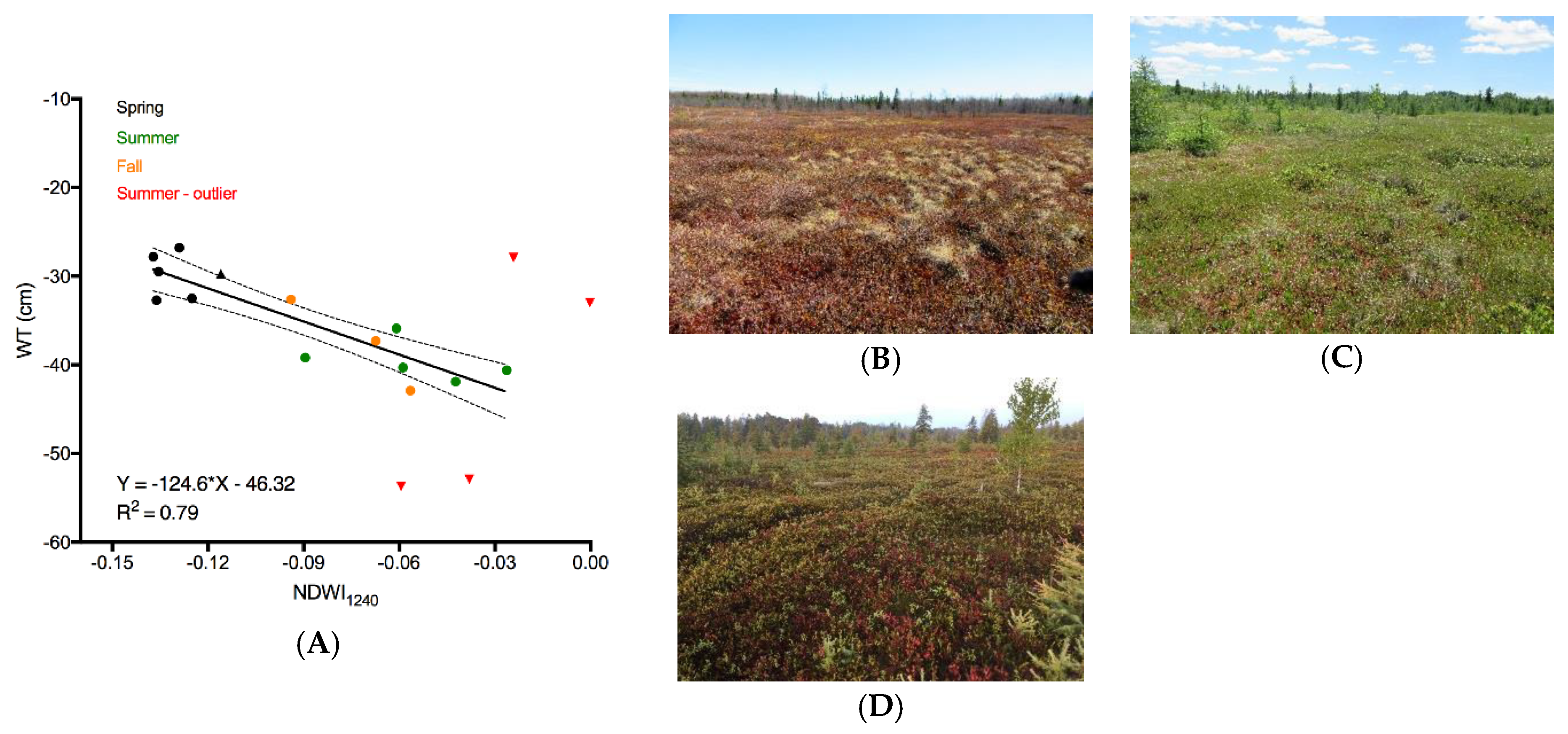
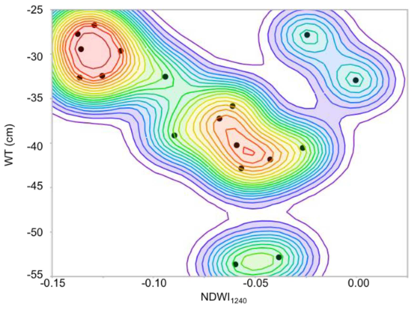
The multitemporal model relating NDWI1240 to water table depth illustrates the sensitivity of the narrowband index to both liquid water content in the vegetation and phenology. Mer Bleue has both deciduous and evergreen vascular plants and there are substantial seasonal variations in nitrogen and chlorophyll concentration in the vascular plants, but not in the mosses [9]. These changes can be seen in multitemporal imagery of the bog [9,51]. With the depth of the water table position having been greater than 20 cm from the surface on the days the SASI HSI were collected over the period of study (2011–2016), the NDWI1240 does not directly observe the position of the water table. The reflectance at these wavelengths is determined solely by the top 3–5 cm of the Sphagnum canopy [57]. While other studies have used exposed surface water to infer the position of the water table across a peatland [58], the relationship here shows NDWI1240 as a proxy for water table position. This is important for Mer Bleue because, other than during exceptionally wet periods, the water table remains below the surface of the hollows [20]. Water table depth is a subdued reflection of the surface microtopography [35], with a strong association to the vegetation community [1]. The magnitude of reflectance at 884.5 nm and 1238.6 nm are indicative of the moisture content in the superficial bog vegetation. As shown by [56], the magnitude of Sphagnum reflectance can vary by as much as 50% in the SWIR region from saturated to dry samples. In particular, the characteristic peaks in reflectance centered between 799–900 nm and 1250–1330 nm in wet Sphagnum are lost as the amplitude of the reflectance in NIR–SWIR increases with drying. Extrapolating the model beyond the range of the WT table depth investigated here should be done with caution because it is unknown if the NDWI1240:WT relationship would remain with very high (i.e., water at surface of hollows) or low (<−43 cm) WT positions. However, at Mer Bleue, a very high WT is rare; it mostly remains below the surface of hollows.
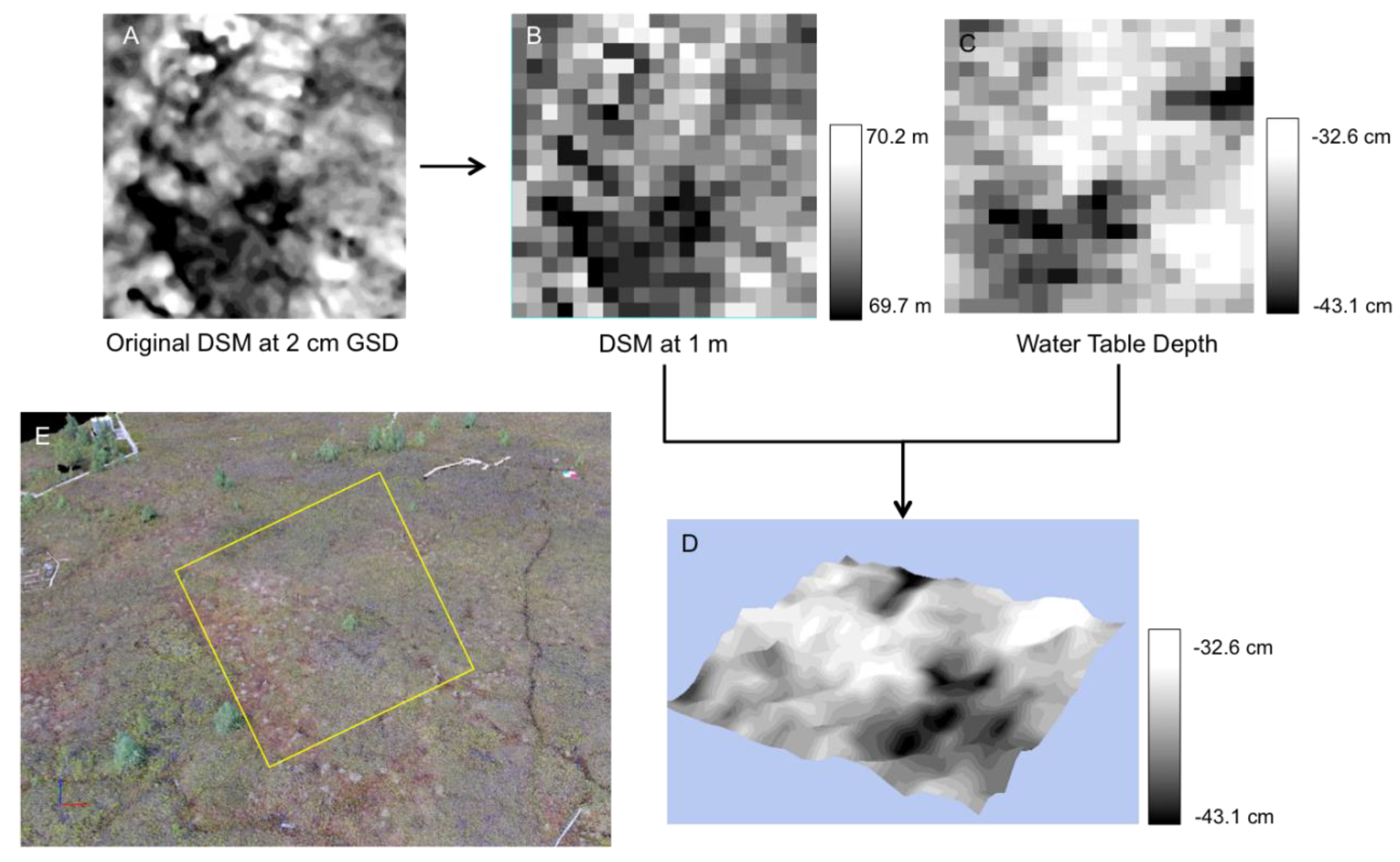
We found a lower correlation between microtopography and water table depth (Figure 6) than [1]. This is due to the spatial resolution (1 m) of the SWIR imagery and the degraded microtopography DSM (2 cm to 1 m). Due to the small spatial scale of the hummocks and hollows, 1 m does not retain their integrity [31], resulting in a mixing of both the elevation and water table at the transition between hummocks and hollows. If these analyses were to be conducted at a finer spatial resolution (e.g., 5 cm), achievable from low-altitude UAV platforms, the correlation between microtopography and water table depth would likely be stronger. Further work investigating this relationship at fine spatial scales is important because UAV-based microtopography modeling is less expensive and more accessible than UAV based SWIR HSI.
Peatland hydrology is one of the most important factors influencing ecology and functioning, with WT depth an important predictor of vegetation structure and composition [28]. In areas with a deeper WT, vascular vegetation in hummocks is taller, with the establishment of trees in areas with the lowest WT [59]. Therefore, long-term changes in the WT depth could alter the spatial distribution and structure of the vascular plants. The position of the WT in the peat profile indicates the depth of the soil air in the pore space, while the vertical range between the surface and the maximum water table depth encompasses the thickness of the acrotelm in which most of the biogeochemical processes take place [28]. Because the roots of many vascular plants require a minimum proportion of soil pore air, temporal monitoring of the WT depth (in a spatial context) could facilitate forecasting succession (i.e., changes in species composition or community structure). The vertical profile of Sphagnum is a dense canopy with spaces and dead hyaline cells of the leaves and branches providing the mechanism for the retention of capillary water above the water table [28]. Lowering of the WT decreases the soil water pressure [60], increasing the possibility of desiccation of the mosses thus resulting in a loss of productivity and carbon sequestration [61]. Substantial lowering of the WT through draining accelerates the decomposition process in the peat and releases of CO2 to the atmosphere [62].
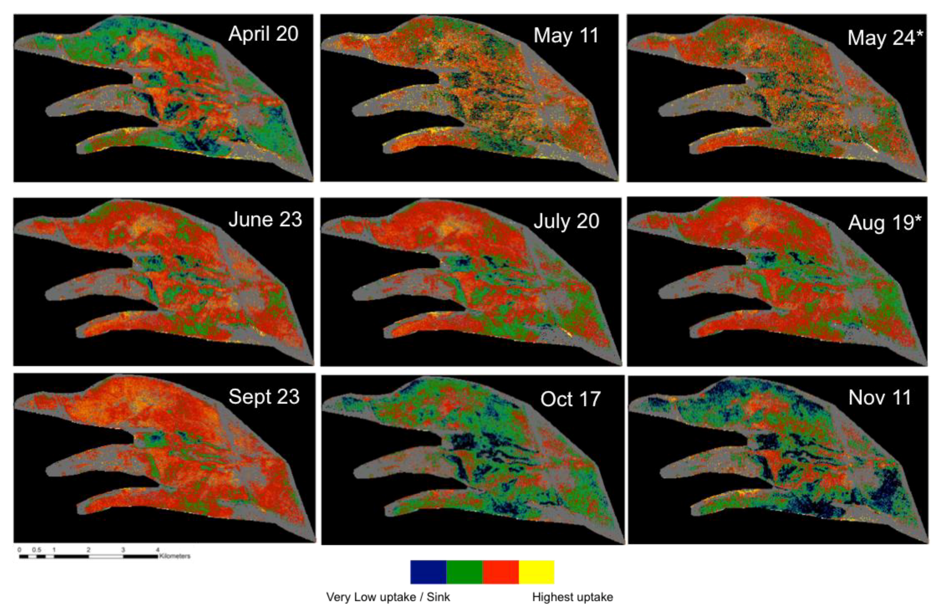
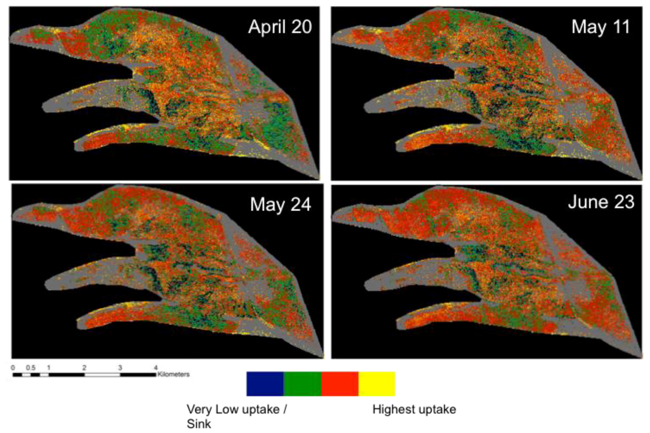
In order to estimate WT with NDWI1240 from airborne HSI, the illumination and acquisition geometries should be carefully considered. As shown in 
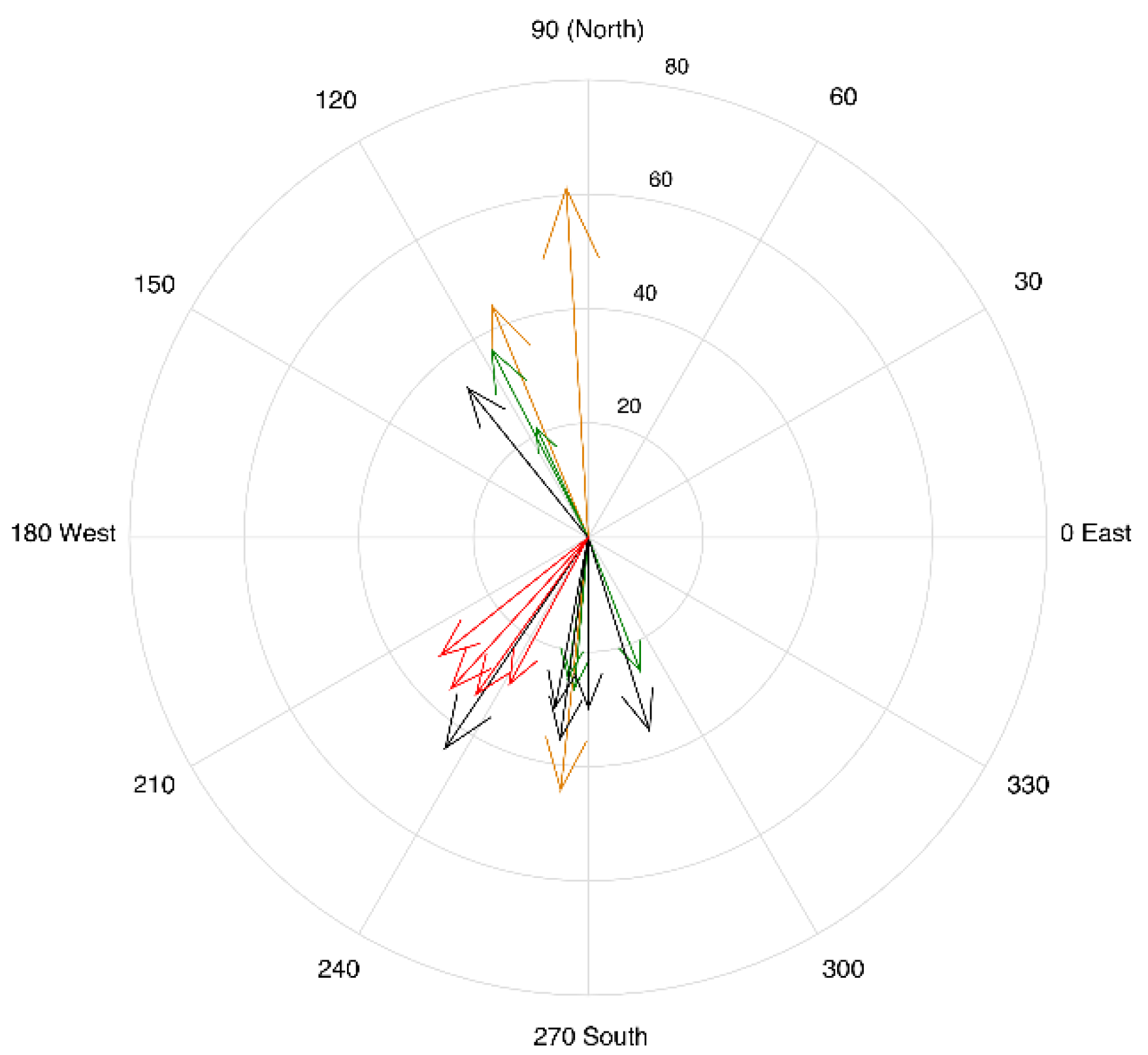
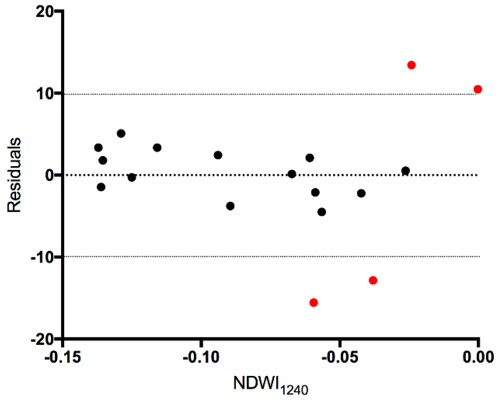
Figure 4, during the summer, with the vascular plants in full foliage, the illumination geometry affects the utility of the image for WT position estimation. The residuals (Figure A1) indicate that the flight lines in the summer (leaf on) with the RAA diagonal to the field of view (128.7–151.8°) were greater than ±10 cm. A non-parametric quantile density plot (Figure A2) further illustrates the dissimilarity between the NDWI1240:WT relationship in these HSI and the rest of the sampling dates. As a result, these four images were not used in the estimation of the WT depth. In contrast, the spring (leaf off) his, with an RAA of 145.9° (black triangle in Figure 3A), was not an outlier in the NDWI1240:WT relationship due to lack of leaves on the vascular plants (Figure 3D and Figure 4). While additional data collection (e.g., HSI collected over a broader range of solar zenith angle (SZA) and SAA throughout the growing season) and analysis are planned to fully understand the reason for this, we believe it is potentially related to the anisotropy of the bog. When reflectance properties of a surface are not perfectly diffuse, they have some degree of anisotropy. This directional characteristic of the surface reflectance when accounted for from all angles is referred to as the bidirectional reflectance distribution function (BRDF) [63]. Vegetation, in general, has long been accepted as having anisotropic reflectance properties [64], however, the majority of studies have focused on modeling and quantifying other ecosystems with minimal studies examining peatlands [65].
Understanding the effects of the anisotropic properties of peatlands on remotely sensed data is important for biogeochemical modeling because transformations applied to reflectance (such as vegetation indices) are strongly affected by BRDF [66]. Goniometer measurements of moss BRDF have indicated that the infrared region showed a greater degree of variability with change in azimuth angle than the visible wavelengths [67]. For moss samples, there was no pronounced hot spot [67]. Instead, the BRDF effects constitute a higher reflectivity perpendicular to the illumination angle at low view angles (similar to illumination conditions found at high latitudes). The BRDF properties of vascular plant canopies are primarily characterized by a hotspot, a peak in reflectance when the sun is directly behind the sensor [61]. At the ecosystem scale, BRDF is a complex process, influenced not only by crown size, density, and spacing between crowns, but also the background soil BRDF, which for peatlands is the moss canopy. Vascular vegetation phenology has also been observed to strongly influence BRDF properties [63,68]. As such, their influence on the overall surface reflectance of the peatland must also be considered.
The broader implication of these observations relates to the mission planning of airborne imagery coincidental with satellite overpasses. At the latitude of Mer Bleue, coincidental image acquisition with Sentinel-2 and Landsat 8 OLI with mission planning aiming to minimize cross-track illumination effects results in suboptimal illumination conditions in the summer (i.e., vascular plants in full foliage) for retrieving biogeochemical properties of the peatland such as near surface water content [31] or WT position relying on SWIR wavelengths. While wavelengths in the VNIR range should be less impacted, allowing for the retrieval of other characteristics such as pigments contents [9], analyses requiring the SWIR region need additional considerations. Application of similar analyses to satellite based SWIR bands (e.g., Sentinel-2 bands 11 and 12) could face comparable challenges without a comprehensive BRDF correction [69].
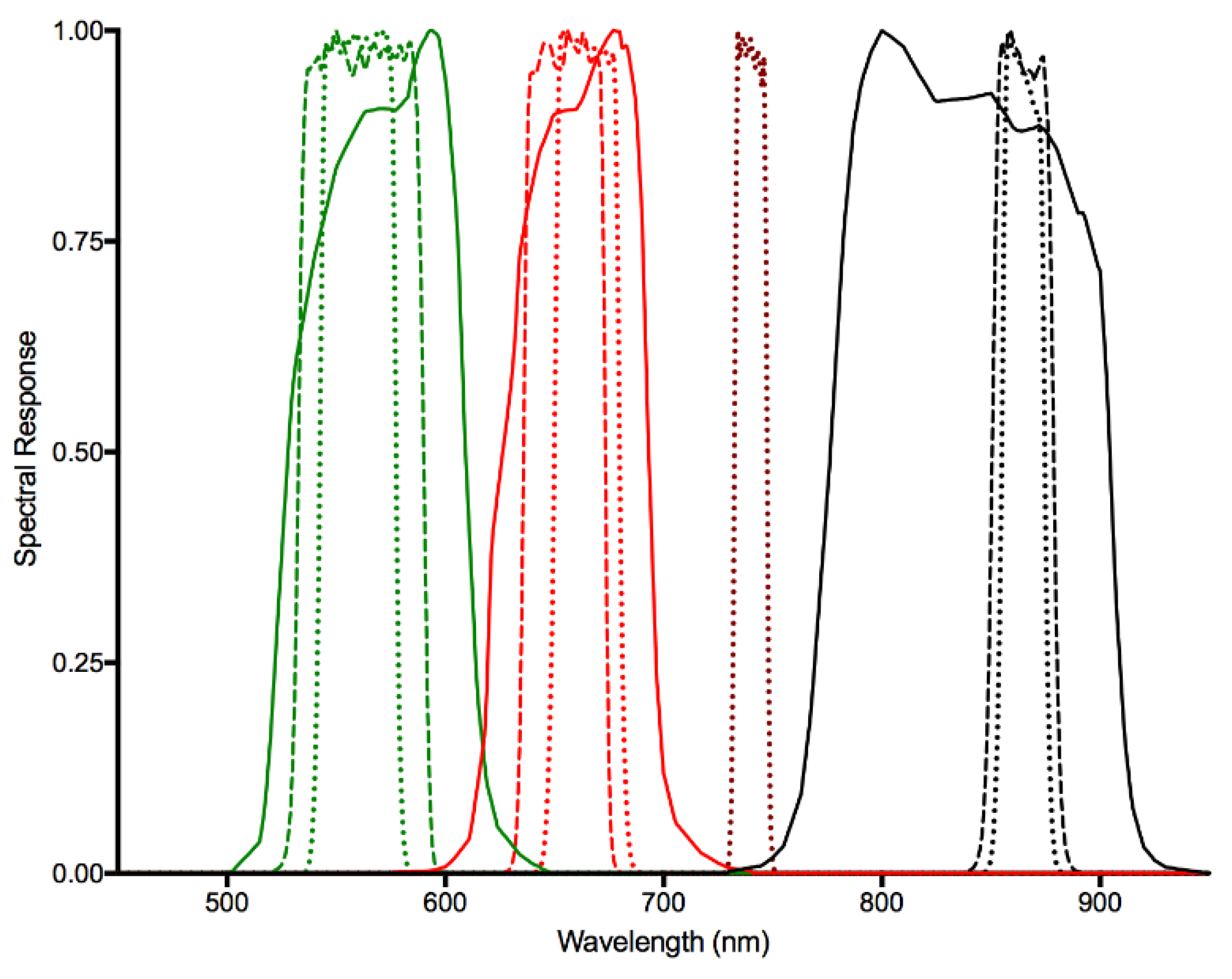
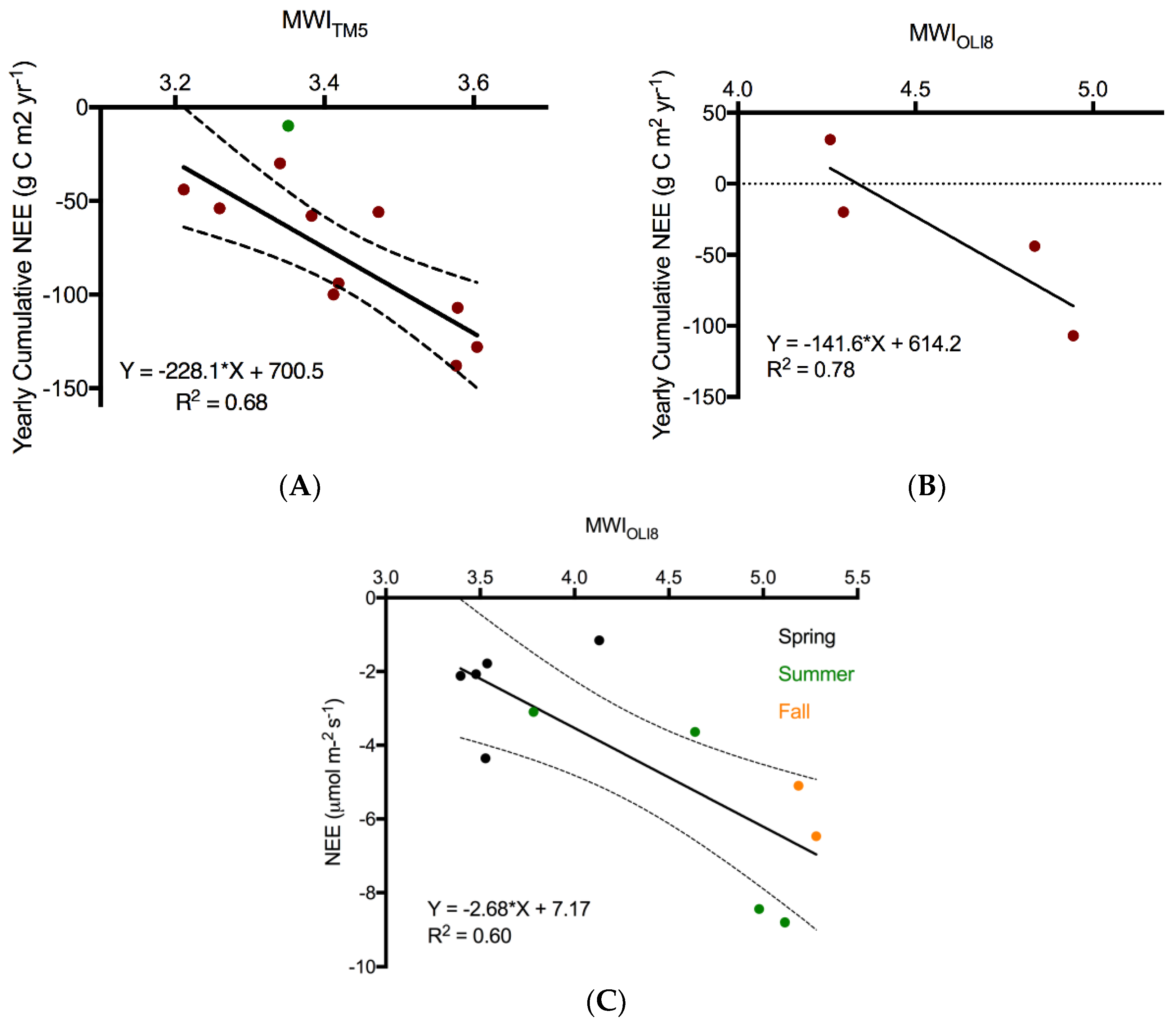
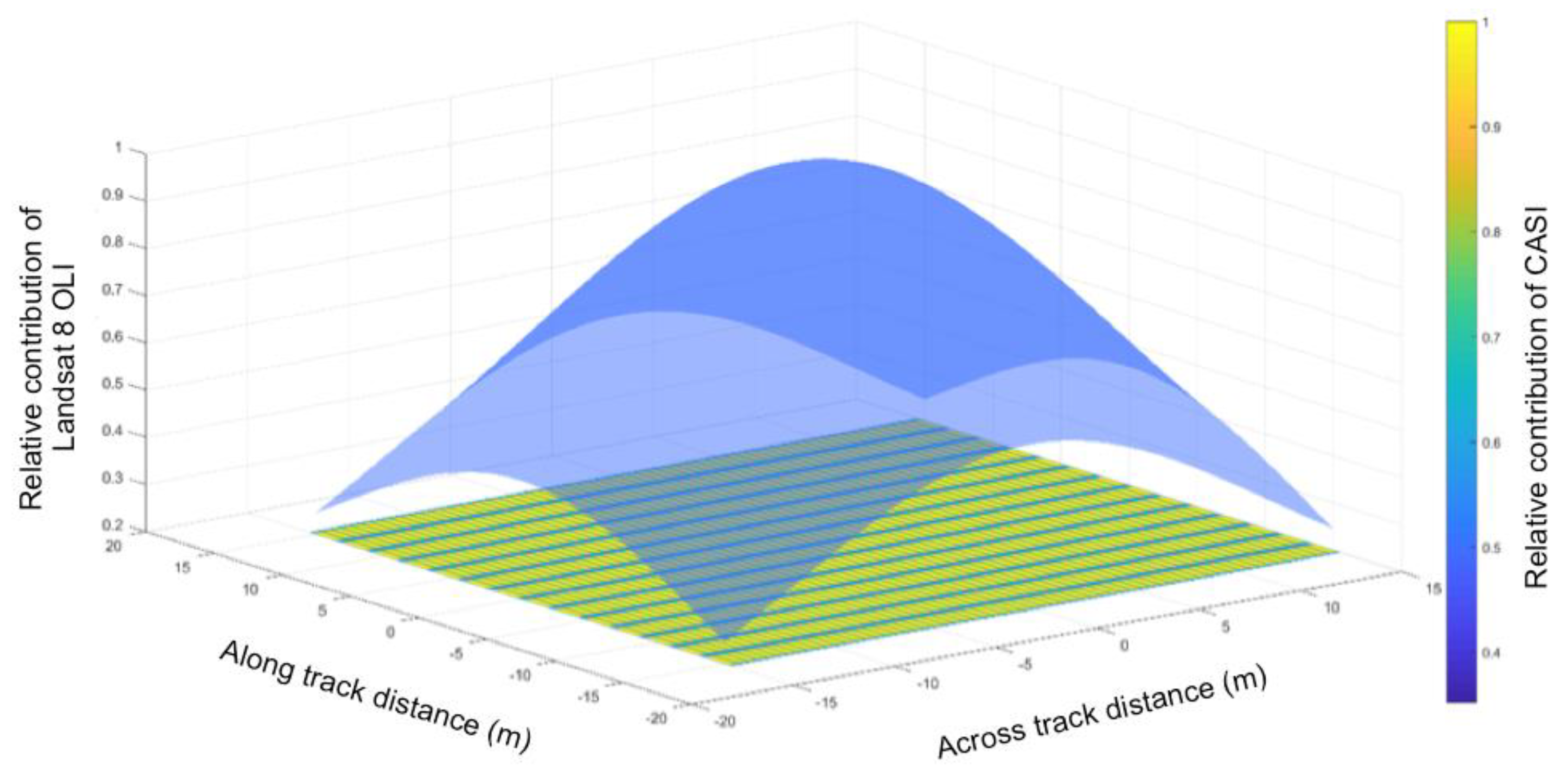
Despite our utilization of the new Collection 1, Tier 1 surface reflectance imagery for the Landsat TM5 and OLI 8 multitemporal models predicting NEE, it was not possible to combine data from the two sensors under our current framework. The fundamental differences in spectral response (Figure 2), spatial response (i.e., line spread functions), radiometry (e.g., SNR, and radiometric resolution), and geometry (location on Earth contributing to the signal) [70] are likely the primary factors in the differences between the models derived from TM5 and OLI8 imagery. Several important changes have been made to the Landsat sensors over the years, resulting in improvements in data quality from Landsat 8 OLI in comparison to its predecessors as described in detail by [70]. However, aside from the obvious spectral resolution differences (Figure 2), we believe two other aspects influencing the specificity of the data acquired are important to consider in this context: instrument design (whiskbroom TM5 vs. pushbroom OLI 8) and radiometric resolution (8 bit TM5 vs. 12 bit OLI 8). The increased dynamic range (from the noise floor to the maximum radiance levels for each band) also leads to an improved noise and quantization performance [71]. The increased radiometric resolution and higher SNR are likely largely responsible for the greater range of MWI from Landsat 8 OLI over a similar range in observed NEE (Figure 8). Experimental degradation of the radiometric resolution of Landsat 8 OLI from 12 to 8 bits illustrated a loss of information at 9 bits, where the distribution of the original 12-bit data was no longer preserved (analysis not shown).
The multiple focal plane array module (FPA) pushbroom design of OLI 8 (and Sentinel-2) replaces the mirror scanning mechanism from Landsat TM5 resulting in, among other characteristics, improved geometric accuracy. However, the stability of the band-to-band registration from the whiskbroom design is more challenging to achieve with the modern sensor approach making use of the multiple FPA pushbroom design [70]. Because the detectors for the different bands are separated in the along-track direction, there is a time delay between the different bands as they image the same location on Earth. For OLI 8, this is estimated to be 1.1 s [70], which results in terrain parallax creating challenges in the removal of high altitude cirrus (i.e., band-to-band registration between the cirrus and optical channels) and changes in satellite position and attitude that must be accounted for to establish the line of sight [44,70,71,72,73,74,75]. Despite efforts to standardize the continuity of land surface products between subsequent generations of satellite sensors [76], our results suggest caution in combining data from sensors with greatly different spectral and radiometric properties for peatland biogeochemical modeling. There is a further consideration of the sensor design related to the offset between the two rows of FPAs in both OLI 8 and Sentinel-2; one set has a slightly forward view of the Earth while the other set has a slightly rearward view [71,72,75]. This is an important consideration for peatlands in the summer, where the vascular plant component has stronger BRDF properties. The difference in the radiance collected by the two sets of FPAs for targets with substantial BRDF properties may be uncorrectable [73], but this effect is mitigated by updated band-specific gain values.
The challenge of removing high-altitude cirrus is seen in our results with the Sentinel-2 imagery from 24 May to 19 August. Full removal of high-altitude cirrus from satellite imagery is not a trivial problem [77,78,79,80,81]. On Landsat 8 OLI, the cirrus band is affected by spectral cross-talk with contamination from the neighboring SWIR band [71] and both Sentinel-2 and Landsat 8 OLI have various magnitudes of band spatial misregistration. This leads to a potential problem for the cirrus removal if the channels have different parallax angles [80,81].
A further consideration requiring more in-depth analyses is that data from all sensors underwent atmospheric correction through different models. Landsat TM5 Collection 1, Tier 1 imagery was atmospherically corrected using the Landsat Ecosystem Disturbance Adaptive Processing System (LEDAPS) [82]. The Landsat 8 OLI Collection 1, Tier 1 imagery was atmospherically corrected using the Landsat Surface Reflectance Code (LaSRC) optimized for Landsat 8 [83]. Sentinel-2A was atmospherically corrected with Sen2cor [45] and the SASI and CASI HSI were atmospherically corrected with ENVI FLAASH 5.4.1 or ATCOR 4.7.0. While there is no comprehensive comparison between these five approaches to atmospheric correction, differences are expected [84]; ATCOR and FLAASH are based on MODTRAN, while LEDAPS and LaRSC implement the MODIS/6S and Vectorial 6S (6SV) models, respectively. Sen2Cor implements a custom algorithm (Sentinel-2 Atmospheric Correction—S2AC) based on the libRadtran4 code [85]. Differences have been shown between the approaches for the two Landsat sensors, where LaSRC processing provides improvements in the surface reflectance over LEDAPS [83]. Similarly, differences have been observed between ATCOR and FLAASH for airborne HSI [86]. However, more extensive comparisons are needed between the HSI and satellite approaches to determine the uncertainty introduced by the different implementations of atmospheric correction and their effect on peatland biogeochemical models.
Finally, our results contribute to the growing body of literature illustrating hyperspectral imagery improves the retrieval of fundamental peatland characteristics over multispectral data at all spatial scales. The HSI used here both have a 14-bit dynamic range. From approximately 1000 m AGL flight altitude, neither the CASI nor SASI were close to saturation; over the peatland only approximately one-third of the dynamic range was utilized. While this may appear to be a cause for concern for low overall SNR, it is not a problem because summation (on- or off-chip) can be used to improve SNR, if needed [38]. The multiple finer spatial pixels (Figure A3) from airborne HSI in comparison to satellite imagery provide a more uniform contribution of the ground elements to the imagery. This is an important consideration for peatlands with fine (≤1 m) spatial structures (e.g., hummocks and hollows). The underutilized dynamic range of the CASI and SASI also suggests that miniaturized versions of the HSI with similar spectral and radiometric properties could be successfully deployed on UAV platforms, where the sensor would be considerably closer to the peatland surface (e.g., <150 m AGL). The higher spatial resolution from UAV-based imagery would benefit WT position models. Planned hyperspectral satellite missions (e.g., EnMap, WaterSat, HyspIRI) could further improve the ongoing remote monitoring of peatlands globally in light of increased pressures from various drivers of change.

5. Conclusions

We successfully modeled WT depth and NEE from airborne hyperspectral and satellite multispectral imagery, respectively. To the best of our knowledge, this is the first time these parameters were retrieved from optical imagery for a peatland at such a fine spatial resolution (1 m for WT depth and 20–30 m for NEE). The narrow band index NDWI1240 was shown to be sensitive to both liquid water content in the vegetation as well as phenology and, therefore, can be used as a proxy for estimating WT depth.
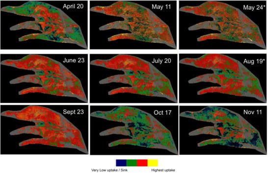
For the retrieval of NEE, we propose separate models, one for historical estimations from Landsat TM5 and a separate model going forward with Landsat 8 OLI or Sentinel-2. We found it was not possible to combine data from sensors with very different spectral and radiometric properties into one model. Despite the successful retrieval of NEE from satellite imagery, the use of airborne HSI improved the relationship with eddy covariance tower-measured NEE. We believe the higher radiometric resolution of the airborne HSI and much finer spatial and spectral resolutions are the reasons for this difference.
The anisotropic properties of the peatland should be considered for the collection of SWIR airborne HSI in the summer when the vascular plants are in full foliage, however, this is less of a concern in the spring prior to green-up. Multitemporal HSI should be collected with consistent illumination and viewing geometries in these types of studies, with the RAA in line with the heading as much as possible. For satellite-based estimations of peatland biogeochemical properties, care must be taken with regards to the detection and removal of high-altitude cirrus. Despite the transparent nature of these clouds, they impact the surface reflectance products, and scenes with cirrus contamination cannot be used to reliably retrieve NEE.
Despite their importance, uncertainties about the total global peatland spatial extent persist, due in part to difficulties in mapping peatlands from coarse resolution remotely sensed data [4,10]. Recent estimates of global peatland extent surpass 4.5 million km2 [4], with over 1 million km2 in both Europe [87] and Canada [3], respectively, based on compilations of national datasets. With the increasing global archives of Landsat and Sentinel-2 imagery, and planetary scale computing platforms, such as Google Earth Engine [42], the methodologies developed here for NEE could be applied to other northern peatlands without tree cover. Ground measurements of NEE from the eddy covariance method should be incorporated to validate the models if applied elsewhere. Global networks such as FLUXNET [88] collect multitemporal data of CO2 exchange that could be used as model training and validation. Protocols being established for satellite-based Land Data Product Validation [89] will allow for greater intercomparability between sites. In the absence of airborne or UAV-based hyperspectral imagery, data from planned spaceborne hyperspectral missions could be investigated to determine their utility for predicting WT depth, provided sufficient in situ data are available to validate the results, especially for WT depth outside the range examined here.
Climate change affects peatlands directly [90,91]. One of the most important drivers of change in the functioning of northern peatlands is the WT depth. Even modest decreases in water table depth coupled with increased air temperature have been shown to lead to profound changes in the proportional contributions of mosses and vascular plants to biomass production [91]. In addition, drought conditions with a lowering of the WT have recently been shown to result in an increase in higher ecosystem respiration, due in part to changes in vegetation composition where vascular plants replaced Sphagnum mosses [90]. Remotely sensed data offer a reliable means to monitor such changes on an ongoing basis.

Author Contributions

Margaret Kalacska and J. Pablo Arroyo-Mora conceived the study; Margaret Kalacska, Raymond J. Soffer and Deep Inamdar processed the imagery; Margaret Kalacska and Raymond J. Soffer analyzed the data; Elyn Humphreys contributed water table and processed eddy covariance tower data; J. Pablo Arroyo-Mora, Raymond J. Soffer and George Leblanc contributed airborne imagery; Nigel T. Roulet and Tim R. Moore interpreted the results and aided in the analysis; George Leblanc acquired the HSI sensors; Oliver Lucanus collected and processed the UAV data; Margaret Kalacska, J. Pablo Arroyo-Mora and Raymond J. Soffer wrote the paper. All authors contributed to the editing of the final manuscript.

Acknowledgments

We acknowledge the funding provided by the European Space Agency (ESA) Sensor Performance, Products and Algorithms (SPPA) element of the Earth Observation ground segment. This work was also supported by the Natural Sciences and Engineering Research Council of Canada (NSERC) and Canada Foundation for Innovation (CFI). We thank Mike Dalva for logistics support at Mer Bleue and Noel Gorelick from Google for help with Google Earth Engine. We express our appreciation to DRDC-Valcartier for the loan of the CASI instrument and to the National Capital Commission for access to Mer Bleue. We thank Jill Bubier, Peter Lafleur and 3 anonymous reviewers for their comments and suggestions to improve the manuscript.

Conflicts of Interest

The authors declare no conflict of interest.

Appendix A

Table A1. Landsat 8 OLI spectral bands from [50].
BandMaximum Bandpass (nm)Spatial Resolution (m)
1 Coastal/Aerosol433–45330
2 Blue450–51530
3 Green525–60030
4 Red630–68030
5 NIR845–88530
6 SWIR11560–166030
7 SWIR22100–230030
PAN500–68015
Cirrus1360–139030
Table A2. Sentinel 2A spectral bands from [43,44].
BandCentral Wavelength (nm)Bandwidth (nm)Spatial Resolution (m)
1 Clouds/aerosols/atm. correction4432760
2 Blue4909810
3 Green5604510
4 Red6653810
5 Red Edge7051920
6 Red Edge7401820
7 NIR7832820
8 NIR84214510
8A NIR8653320
9 NIR9402660
10 Cirrus13757560
11 SWIR161014320
12 SWIR219024220
Figure A1. Residuals form the NDWI1240:WT relationship. The four summer leaf-on HSI collected with the greatest deviation from solar noon (red) have residual values in excess of ±10 cm.
Remotesensing 10 00687 g0a1
Figure A2. Bivariate quantile density plot of the NDWI1240:WT relationship. Each contour line represents a quantile contour in 5% increments. Red lines are a quantile density of 0.9 and purple are 0.1. The four points referred to as outliers from Figure 3A and Figure 4 can be seen above and below main group of 14 points.
Remotesensing 10 00687 g0a2
Figure A3. Relative contribution of a 30 × 30 m area to a Landsat 8 OLI pixel and the CASI HSI covering same area. The 3D spatial response function in transparent blue illustrates the Landsat 8 OLI line spread function at full width half maximum (FWHM) from prelaunch measurements [70]. The heat map of the CASI line spread function at FWHM is illustrated for a flight conducted at 1000 m altitude and 80 knots.
Remotesensing 10 00687 g0a3

References

  1. Malhotra, A.; Roulet, N.T.; Wilson, P.; Giroux-Bougard, X.; Harris, L.I. Ecohydrological feedbacks in peatlands: An empirical test of the relationship among vegetation, microtopography and water table. Ecohydrology 2016, 9, 1346–1357. [Google Scholar] [CrossRef]
  2. Loisel, J.; Yu, Z.C.; Beilman, D.W.; Camill, P.; Alm, J.; Amesbury, M.J.; Anderson, D.; Andersson, S.; Bochicchio, C.; Barber, K.; et al. A database and synthesis of northern peatland soil properties and Holocene carbon and nitrogen accumulation. Holocene 2014, 24, 1028–1042. [Google Scholar] [CrossRef] [Green Version]
  3. Tarnocai, C.; Kettles, I.M.; Lacelle, B. Peatlands of Canada Database; Agriculture and Agri-Food Canada: Ottawa, ON, Canada, 2005. [Google Scholar]
  4. Leifeld, J.; Menichetti, L. The underappreciated potential of peatlands in global climate change mitigation strategies. Nat. Commun. 2018, 9, 1071. [Google Scholar] [CrossRef] [PubMed]
  5. Fenner, N.; Freeman, C. Drought-induced carbon loss in peatlands. Nat. Geosci. 2011, 4, 895–900. [Google Scholar] [CrossRef]
  6. Yu, Z.C.; Campbell, I.D.; Campbell, C.; Vitt, D.H.; Bond, G.C.; Apps, M.J. Carbon sequestration in western Canadian peat highly sensitive to Holocene wet-dry climate cycles at millennial timescales. Holocene 2003, 13, 801–808. [Google Scholar] [CrossRef]
  7. Harris, A.; Bryant, R.G. A multi-scale remote sensing approach for monitoring northern peatland hydrology: Present possibilities and future challenges. J. Environ. Manag. 2009, 90, 2178–2188. [Google Scholar] [CrossRef] [PubMed]
  8. Harris, A.; Bryant, R.G.; Baird, A.J. Mapping the effects of water stress on Sphagnum: Preliminary observations using airborne remote sensing. Remote Sens. Environ. 2006, 100, 363–378. [Google Scholar] [CrossRef]
  9. Kalacska, M.; Lalonde, M.; Moore, T.R. Estimation of foliar chlorophyll and nitrogen content in an ombrotrophic bog from hyperspectral data: Scaling from leaf to image. Remote Sens. Environ. 2015, 169, 270–279. [Google Scholar] [CrossRef]
  10. Krankina, O.N.; Pflugmacher, D.; Friedl, M.; Cohen, W.B.; Nelson, P.; Baccini, A. Meeting the challenge of mapping peatlands with remotely sensed data. Biogeosciences 2008, 5, 1809–1820. [Google Scholar] [CrossRef]
  11. Sonnentag, O.; Chen, J.M.; Roberts, D.A.; Talbot, J.; Halligan, K.Q.; Govind, A. Mapping tree and shrub leaf area indices in an ombrotrophic peatland through multiple endmember spectral unmixing. Remote Sens. Environ. 2007, 109, 342–360. [Google Scholar] [CrossRef]
  12. Arroyo-Mora, J.P.; Kalacska, M.; Lucanus, O.; Soffer, R.J.S.; Leblanc, G. Spectro-spatial relationship between UAV derived high resolution DEM and SWIR hyperspectral data: Application to an ombrotrophic peatland. In Proceedings of the SPIE Remote Sensing, Warsaw, Poland, 11–14 September 2017. [Google Scholar]
  13. Bubier, J.L.; Rock, B.N.; Crill, P.M. Spectral reflectance measurements of boreal wetland and forest mosses. J. Geophys. Res. Atmos. 1997, 102, 29483–29494. [Google Scholar] [CrossRef]
  14. Gao, B.-C. NDWI—A normalized difference water index for remote sensing vegetation liquid water from space. Remote Sens. Environ. 1996, 58, 257–266. [Google Scholar] [CrossRef]
  15. Meingast, K.M.; Falkowski, M.J.; Kane, E.S.; Potvin, L.R.; Benscoter, B.W.; Smith, A.M.S.; Bourgeau-Chavez, L.L.; Miller, M.E. Spectral detection of near-surface moisture content and water-table position in northern peatland ecosystems. Remote Sens. Environ. 2014, 152, 536–546. [Google Scholar] [CrossRef]
  16. Lund, M.; Lafleur, P.M.; Roulet, N.T.; Lindroth, A.; Christensen, T.R.; Aurela, M.; Chojnicki, B.H.; Flanagan, L.B.; Humphreys, E.R.; Laurila, T.; et al. Variability in exchange of CO2 across 12 northern peatland and tundra sites. Glob. Chang. Biol. 2010, 16, 2436–2448. [Google Scholar] [CrossRef]
  17. Juutinen, S.; Bubier, J.L.; Moore, T.R. Responses of vegetation and ecosystem CO2 exchange to 9 Years of nutrient addition at Mer Bleue bog. Ecosystems 2010, 13, 874–887. [Google Scholar] [CrossRef]
  18. Adkinson, A.C.; Humphreys, E.R. The response of carbon dioxide exchange to manipulations of Sphagnum water content in an ombrotrophic bog. Ecohydrology 2011, 4, 733–743. [Google Scholar] [CrossRef]
  19. Aurela, M.; Tuovinen, J.P.; Laurila, T. Carbon dioxide exchange in a subarctic peatland ecosystem in northern Europe measured by the eddy covariance technique. J. Geophys. Res. Atmos. 1998, 103, 11289–11301. [Google Scholar] [CrossRef]
  20. Lafleur, P.M.; Roulet, N.T.; Bubier, J.; Frolking, S.; Moore, T.R. Interannual variability in the peatland-atmosphere carbon dioxide exchange at an ombrotrophic bog. Glob. Biogeochem. Cycles 2003, 17, 13. [Google Scholar] [CrossRef]
  21. Kross, A.; Seaquist, J.W.; Roulet, N.T.; Fernandes, R.; Sonnentag, O. Estimating carbon dioxide exchange rates at contrasting northern peatlands using MODIS satellite data. Remote Sens. Environ. 2013, 137, 234–243. [Google Scholar] [CrossRef]
  22. Schubert, P.; Eklundh, L.; Lund, M.; Nilsson, M. Estimating northern peatland CO2 exchange from MODIS time series data. Remote Sens. Environ. 2010, 114, 1178–1189. [Google Scholar] [CrossRef]
  23. Crichton, K.A.; Anderson, K.; Bennie, J.J.; Milton, E.J. Characterizing peatland carbon balance estimates using freely available Landsat ETM plus data. Ecohydrology 2015, 8, 493–503. [Google Scholar] [CrossRef]
  24. Lees, K.J.; Quaife, T.; Artz, R.R.E.; Khomik, M.; Clark, J.M. Potential for using remote sensing to estimate carbon fluxes across northern peatlands—A review. Sci. Total Environ. 2018, 615, 857–874. [Google Scholar] [CrossRef] [PubMed]
  25. Holden, J. Peatland hydrology and carbon release: Why small-scale process matters. Philos. Trans. R. Soc. A Math. Phys. Eng. Sci. 2005, 363, 2891–2913. [Google Scholar] [CrossRef] [PubMed]
  26. Moore, T.R.; De Young, A.; Bubier, J.L.; Humphreys, E.R.; Lafleur, P.M.; Roulet, N.T. A multi-year record of methane flux at the Mer Bleue bog, southern Canada. Ecosystems 2011, 14, 646–657. [Google Scholar] [CrossRef]
  27. Williams, T.G.; Flanagan, L.B. Effect of changes in water content on photosynthesis, transpiration and discrimination against (CO2)-C-13 and (COO)-O-18-O-16 in Pleurozium and Sphagnum. Oecologia 1996, 108, 38–46. [Google Scholar] [CrossRef] [PubMed]
  28. Rydin, H.; Jeglum, J.K. The Biology of Peatlands; Oxford University Press: Oxford, UK, 2013. [Google Scholar]
  29. Kross, A.S.E.; Roulet, N.T.; Moore, T.R.; Lafleur, P.M.; Humphreys, E.R.; Seaquist, J.W.; Flanagan, L.B.; Aurela, M. Phenology and its role in carbon dioxide exchange processes in northern peatlands. J. Geophys. Res. Biogeosci. 2014, 119, 1370–1384. [Google Scholar] [CrossRef]
  30. Moore, T.R.; Lafleur, P.M.; Poon, D.M.I.; Heumann, B.W.; Seaquist, J.W.; Roulet, N.T. Spring photosynthesis in a cool temperate bog. Glob. Chang. Biol. 2006, 12, 2323–2335. [Google Scholar] [CrossRef]
  31. Arroyo-Mora, J.P.; Kalacska, M.; Soffer, R.J.S.; Moore, T.R.; Roulet, N.T.; Juutinen, S.; Ifimov, G.; Leblanc, G.; Inamdar, D. Airborne hyperspectral evaluation of maximum gross photosynthesis, gravimetric water content and CO2 uptake efficiency of the Mer Bleue ombrotrophic peatland. Remote Sens. 2018, 10, 565. [Google Scholar] [CrossRef]
  32. Bilali, H.; Patterson, T.; Prokoph, A. A Holocene paleoclimate reconstruction for eastern Canada based on δ18O cellulose of Sphagnum mosses from Mer Bleue Bog. Holocene 2013, 23, 1260–1271. [Google Scholar] [CrossRef]
  33. Roulet, N.T.; Lafleur, P.M.; Richard, P.J.H.; Moore, T.R.; Humphreys, E.; Bubier, J. Contemporary carbon balance and late Holocene carbon accumulation in a northern peatland. Glob. Chang. Biol. 2007, 13, 397–411. [Google Scholar] [CrossRef]
  34. Lafleur, P.M.; Moore, T.R.; Roulet, N.T.; Frolking, S. Ecosystem respiration in a cool temperate bog depends on peat temperature but not water table. Ecosystems 2005, 8, 619–629. [Google Scholar] [CrossRef]
  35. Wilson, P. The Relationship among Micro-Topographic Variation, Water Table Depth and Biogeochemistry in an Ombrotrophic Bog; McGill University: Montreal, QC, Canada, 2012. [Google Scholar]
  36. Moore, T.R.; Bubier, J.; Frolking, S.; Lafleur, P.M.; Roulet, N.T. Plant biomass and production and CO2 exchange in an ombrotrophic bog. J. Ecol. 2002, 90, 25–36. [Google Scholar] [CrossRef]
  37. Lafleur, P.M.; Roulet, N.T.; Admiral, S.W. Annual cycle of CO2 exchange at a bog peatland. J. Geophys. Res. Atmos. 2001, 106, 3071–3081. [Google Scholar] [CrossRef]
  38. Kalacska, M.; Arroyo-Mora, J.P.; Soffer, R.J.S.; Leblanc, G. Quality control assessment of the mission airborne carbon 13 (mac-13) hyperspectral imagery from Costa Rica. Can. J. Remote Sens. 2016, 42, 85–105. [Google Scholar] [CrossRef]
  39. Soffer, R.J.S.; Arroyo-Mora, J.P.; Kalacska, M.; Ifimov, G.; White, P.H.; Leblanc, S.; Nazarenko, D.; Leblanc, G. MBASSS Sentinel -2, Landsat 8 Data Product Validation Project – Final Report; National Research Council of Canada: Ottawa, ON, Canada, 2017; p. 285. [Google Scholar]
  40. ITRES. Standard Processing and Data QA Manual; ITRES Research Ltd.: Calgary, AB, Canada, 2013; p. 182. [Google Scholar]
  41. Allux, S.; Leblanc, G. Post-Radiometric Processing of SASI Hyperspectral Data; National Research Council of Canada: Ottawa, ON, Canada, 2010. [Google Scholar]
  42. Gorelick, N.; Hancher, M.; Dixon, M.; Ilyushchenko, S.; Thau, D.; Moore, R. Google Earth Engine: Planetary-scale geospatial analysis for everyone. Remote Sens. Environ. 2017, 202, 18–27. [Google Scholar] [CrossRef]
  43. European Space Agency. Sentinel-2 User Handbook; European Space Agency: Paris, France, 2015; p. 64. [Google Scholar]
  44. Gascon, F.; Thepaut, O.; Jung, M.; Francesconi, B.; Louis, J.; Lonjou, V.; Lafrance, B.; Massera, S.; Gaudel-Vacaresse, A.; Languille, F.; et al. Copernicus Sentinel-2 Calibration and Products Validation Status. Remote Sens. 2017, 9, 584. [Google Scholar] [CrossRef]
  45. Müller-Wilm, U. Sentinel-2 MSI – Level-2A Prototype Processor Installation and User Manual; Telespazio VEGA Deutschland GmbH: Darmstadt, Germany, 2016; p. 51. [Google Scholar]
  46. Connolly, J.; Roulet, N.T.; Seaquist, J.W.; Holden, N.M.; Lafleur, P.M.; Humphreys, E.R.; Heumann, B.W.; Ward, S.M. Using MODIS derived fPAR with ground based flux tower measurements to derive the light use efficiency for two Canadian peatlands. Biogeosciences 2009, 6, 225–234. [Google Scholar] [CrossRef]
  47. Teklemariam, T.A.; Lafleur, P.M.; Moore, T.R.; Roulet, N.T.; Humphreys, E.R. The direct and indirect effects of inter-annual meteorological variability on ecosystem carbon dioxide exchange at a temperate ombrotrophic bog. Agric. For. Meteorol. 2010, 150, 1402–1411. [Google Scholar] [CrossRef]
  48. Kalacska, M.; Lucanus, O.; Arroyo-Mora, J.P. 30-Year Global Surface Water Change: Implications for Aquatic Diversity; ESRI User Summit: San Diego, CA, USA, 2017. [Google Scholar]
  49. NASA Landsat Science Landsat 5. Available online: https://landsat.gsfc.nasa.gov/landsat-5/ (accessed on 5 February 2018).
  50. Barsi, J.A.; Lee, K.; Kvaran, G.; Markham, B.L.; Pedelty, J.A. The Spectral Response of the Landsat-8 Operational Land Imager. Remote Sens. 2014, 6, 10232–10251. [Google Scholar] [CrossRef]
  51. Arroyo-Mora, J.P.; Kalacska, M.; Soffer, R.J.S.; Ifimov, G.; Leblanc, G.; Schaaf, E.S.; Lucanus, O. Phenospectral dynamics of vegetation physiognomies at different spatial and spectral scales at the Mer Bleue ombrotrophic peatland. Remote Sens. Environ. under review 2017.
  52. Prairie, Y.T. Evaluating the predictive power of regression models. Can. J. Fish. Aquat. Sci. 1996, 53, 490–492. [Google Scholar] [CrossRef]
  53. Schipperges, B.; Rydin, H. Response of photosynthesis of Sphagnum species from contrasting microhabitats to tissue water content and repeated desiccation. New Phytol. 1998, 140, 677–684. [Google Scholar] [CrossRef]
  54. St-Hilaire, F.; Wu, J.; Roulet, N.T.; Frolking, S.; Lafleur, P.M.; Humphreys, E.R.; Arora, V. McGill wetland model: Evaluation of a peatland carbon simulator developed for global assessments. Biogeosciences 2010, 7, 3517–3530. [Google Scholar] [CrossRef] [Green Version]
  55. Wu, J.H.; Roulet, N.T.; Nilsson, M.; Lafleur, P.; Humphreys, E. Simulating the carbon cycling of northern peatlands using a Land Surface Scheme coupled to a Wetland Carbon Model (CLASS3W-MWM). Atmos. Ocean 2012, 50, 487–506. [Google Scholar] [CrossRef]
  56. Bryant, R.G.; Baird, A.J. The spectral behaviour of Sphagnum canopies under varying hydrological conditions. Geophys. Res. Lett. 2003, 30. [Google Scholar] [CrossRef]
  57. Lalonde, M. The Hyperspectral Determination of Sphagnum Water Content in a Bog; McGill University: Montreal, QC, Canada, 2014. [Google Scholar]
  58. Rahman, M.M.; McDermid, G.J.; Strack, M.; Lovitt, J. A new method to map groundwater table in peatlands using unmanned aerial vehicles. Remote Sens. 2017, 9, 1057. [Google Scholar] [CrossRef]
  59. Verry, E.S. Hydrological processes of natural, northern forested wetlands. In Northern Forested Wetlands Ecology and Management; Tretin, C.C., Jurgensen, M.F., Grigal, D.F., Gale, M.R., Jeglum, J.K., Eds.; CRC Press: Boca Raton, FL, USA, 1997; pp. 163–188. [Google Scholar]
  60. Dimitrov, D.D.; Grant, R.F.; Lafleur, P.M.; Humphreys, E.R. Modeling the effects of hydrology on gross primary productivity and net ecosystem productivity at Mer Bleue bog. J. Geophys. Res. Biogeosci. 2011, 116. [Google Scholar] [CrossRef]
  61. Dixon, S.J.; Kettridge, N.; Moore, P.A.; Devito, K.J.; Tilak, A.S.; Petrone, R.M.; Mendoza, C.A.; Waddington, J.M. Peat depth as a control on moss water availability under evaporative stress. Hydrol. Process. 2017, 31, 4107–4121. [Google Scholar] [CrossRef]
  62. Rubec, C.D.A. Policy for conservation of the functions and values of forested wetlands. In Northern Forested Wetlands Ecology and Management; Tretin, C.C., Jurgensen, M.F., Grigal, D.F., Gale, M.R., Jeglum, J.K., Eds.; CRC Press: Boca Raton, FL, USA, 1997; pp. 46–58. [Google Scholar]
  63. Gatebe, C.K.; King, M.D. Airborne spectral BRDF of various surface types (ocean, vegetation, snow, desert, wetlands, cloud decks, smoke layers) for remote sensing applications. Remote Sens. Environ. 2016, 179, 131–148. [Google Scholar] [CrossRef]
  64. Peddle, D.R.; Brunke, S.P.; Hall, F.G. A comparison of spectral mixture analysis and ten vegetation indices for estimating boreal forest biophysical information from airborne data. Can. J. Remote Sens. 2001, 27, 627–635. [Google Scholar] [CrossRef]
  65. Coburn, C.A.; Van Gaalen, E.; Peddle, D.R.; Flanagan, L.B. Anisotropic reflectance effects on spectral indices for estimating ecophysiological parameters using a portable goniometer system. Can. J. Remote Sens. 2010, 36, 355–364. [Google Scholar] [CrossRef]
  66. Nagol, J.R.; Sexton, J.; Kim, D.H.; Anand, A.; Morton, D.; Vermote, E.; Townshend, J.R. Bidirectional effects in Landsat reflectance estimates: Is there a problem to solve? ISPRS J. Photogramm. Remote Sens. 2015, 103, 129–135. [Google Scholar] [CrossRef]
  67. Coburn, C.A.; Peddle, D.R. A low-cost field and laboratory goniometer system for estimating hyperspectral bidirectional reflectance. Can. J. Remote Sens. 2006, 32, 244–253. [Google Scholar] [CrossRef]
  68. Bhandari, S.; Phinn, S.; Gill, T. Assessing viewing and illumination geometry effects on the MODIS vegetation index (MOD13Q1) time series: Implications for monitoring phenology and disturbances in forest communities in Queensland, Australia. Int. J. Remote Sens. 2011, 32, 7513–7538. [Google Scholar] [CrossRef]
  69. Roy, D.P.; Li, J.; Zhang, H.K.; Yan, L.; Huang, H.; Li, Z. Examination of Sentinel-2A multi-spectral instrument (MSI) reflectance anisotropy and the suitability of a general method to normalize MSI reflectance to nadir BRDF adjusted reflectance. Remote Sens. Environ. 2017, 199, 25–38. [Google Scholar] [CrossRef]
  70. Markham, B.L.; Arvidson, T.; Barsi, J.A.; Choate, M.; Kaita, E.; Levy, R.; Lubke, M.; Masek, J.G. Landsat Program. In Comprehensive Remote Sensing; Missions and Sensors; Liang, S., Xiong, X., Butler, J.J., Eds.; Elsevier: New York, NY, USA, 2018; Volume 1, pp. 27–90. [Google Scholar]
  71. Morfitt, R.; Barsi, J.; Levy, R.; Markham, B.; Micijevic, E.; Ong, L.; Scaramuzza, P.; Vanderwerff, K. Landsat-8 Operational Land Imager (OLI) Radiometric Performance On-Orbit. Remote Sens. 2015, 7, 2208–2237. [Google Scholar] [CrossRef]
  72. Pahlevan, N.; Sarkar, S.; Franz, B.A.; Balasubramanian, S.V.; He, J. Sentinel-2 MultiSpectral Instrument (MSI) data processing for aquatic science applications: Demonstrations and validations. Remote Sens. Environ. 2017, 201, 47–56. [Google Scholar] [CrossRef]
  73. Pahlevan, N.; Schott, J.R.; Franz, B.A.; Zibordi, G.; Markham, B.; Bailey, S.; Schaaf, C.B.; Ondrusek, M.; Greb, S.; Strait, C.M. Landsat 8 remote sensing reflectance (Rrs) products: Evaluations, intercomparisons, and enhancements. Remote Sens. Environ. 2017, 190, 289–301. [Google Scholar] [CrossRef]
  74. Storey, J.; Choate, M.; Lee, K. Landsat 8 Operational Land Imager On-Orbit Geometric Calibration and Performance. Remote Sens. 2014, 6, 11127–11152. [Google Scholar] [CrossRef]
  75. Storey, J.; Roy, D.P.; Masek, J.; Gascon, F.; Dwyer, J.; Choate, M. A note on the temporary misregistration of Landsat-8 Operational Land Imager (OLI) and Sentinel-2 Multi Spectral Instrument (MSI) imagery. Remote Sens. Environ. 2016, 186, 121–122. [Google Scholar] [CrossRef]
  76. Roy, D.P.; Kovalskyy, V.; Zhang, H.K.; Vermote, E.F.; Yan, L.; Kumar, S.S.; Egorov, A. Characterization of Landsat-7 to Landsat-8 reflective wavelength and normalized difference vegetation index continuity. Remote Sens. Environ. 2016, 185, 57–70. [Google Scholar] [CrossRef]
  77. Bachmann, M.; Makarau, A.; Segl, K.; Richter, R. Estimating the influence of spectral and radiometric calibration uncertainties on EnMAP data products—Examples for ground reflectance retrieval and vegetation indices. Remote Sens. 2015, 7, 10689–10714. [Google Scholar] [CrossRef] [Green Version]
  78. Bendor, E. A precaution regarding cirrus cloud detection from airborne imaging spectrometer data using the 1.38 μm water-vapor band. Remote Sens. Environ. 1994, 50, 346–350. [Google Scholar] [CrossRef]
  79. Gao, B.C.; Goetz, A.F.H.; Wiscombe, W.J. Cirrus cloud detection from airborne imaging spectrometer data using the 1.38 μm water-vapor band. Geophys. Res. Lett. 1993, 20, 301–304. [Google Scholar] [CrossRef]
  80. Gao, B.C.; Li, R.R. Removal of thin cirrus scattering effects in Landsat 8 OLI images using the cirrus detecting channel. Remote Sens. 2017, 9, 10. [Google Scholar] [CrossRef]
  81. Richter, R.; Wang, X.J.; Bachmann, M.; Schlapfer, D. Correction of cirrus effects in Sentinel-2 type of imagery. Int. J. Remote Sens. 2011, 32, 2931–2941. [Google Scholar] [CrossRef]
  82. Masek, J.G.; Vermote, E.F.; Saleous, N.E.; Wolfe, R.; Hall, F.G.; Huemmrich, K.F.; Gao, F.; Kutler, J.; Lim, T.K. A Landsat surface reflectance dataset for North America, 1990-2000. IEEE Geosci. Remote Sens. Lett. 2006, 3, 68–72. [Google Scholar] [CrossRef]
  83. Vermote, E.; Justice, C.; Claverie, M.; Franch, B. Preliminary analysis of the performance of the Landsat 8/OLI land surface reflectance product. Remote Sens. Environ. 2016, 185, 46–56. [Google Scholar] [CrossRef]
  84. Doxani, G.; Vermote, E.; Roger, J.-C.; Gascon, F.; Adriaensen, S.; Frantz, D.; Hagolle, O.; Hollstein, A.; Kirches, G.; Li, F.; et al. Atmospheric Correction Inter-Comparison Exercise. Remote Sens. 2018, 10, 352. [Google Scholar] [CrossRef]
  85. Richter, R.; Berthelot, J.L.B. Sentinel-2 MSI – Level 2A Products Algorithm Theoretical Basis Document. Available online: https://earth.esa.int/c/document_library/get_file?folderId=349490&name=DLFE-4518.pdf (accessed on 23 April 2018).
  86. Kalacska, M.; Arroyo-Mora, J.P.; Soffer, R.J.S. Atmospheric correction of airborne hyperspectral imagery in diverse tropical ecosystems—Lessons learned from Mission Airborne Carbon 13. In Proceedings of the Canadian Symposium on Remote Sensing, St. John’s, NL, Canada, 8–11 June 2015. [Google Scholar]
  87. Tanneberger, F.; Tegetmeyer, C.; Busse, S.; Barthelmes, A.; Shumka, S.; Moles Mariné, A.; Jenderedjian, K.; Steiner, G.M.; Essl, F.; Etzold, J.; et al. The peatland map of europe. Mires Peat 2017, 19, 1–17. [Google Scholar]
  88. Baldocchi, D.; Chu, H.S.; Reichstein, M. Inter-annual variability of net and gross ecosystem carbon fluxes: A review. Agric. For. Meteorol. 2018, 249, 520–533. [Google Scholar] [CrossRef]
  89. Committee on Earth Observation Satellites. Land Product Validation Subgroup. Available online: https://lpvs.gsfc.nasa.gov/documents.html (accessed on 23 April 2018).
  90. Jassey, V.E.J.; Reczuga, M.K.; Zielińska, M.; Słowińska, S.; Robroek, B.J.M.; Mariotte, P.; Seppey, C.V.W.; Lara, E.; Barabach, J.; Słowiński, M.; et al. Tipping point in plant–fungal interactions under severe drought causes abrupt rise in peatland ecosystem respiration. Glob. Chang. Biol. 2018, 24, 972–986. [Google Scholar] [CrossRef] [PubMed]
  91. Mäkiranta, P.; Laiho, R.; Mehtätalo, L.; Straková, P.; Sormunen, J.; Minkkinen, K.; Penttilä, T.; Fritze, H.; Tuittila, E.-S. Responses of phenology and biomass production of boreal fens to climate warming under different water-table level regimes. Glob. Chang. Biol. 2018, 24, 944–956. [Google Scholar] [CrossRef] [PubMed]
Figure 1. (A) Shortwave airborne spectrographic imager (SASI) shortwave infrared (SWIR) hyperspectral imagery (HSI) mosaic of 12 flight lines acquired 24 May 2016 (R: 1052 nm G: 1624 nm B: 2122 nm) illustrating the entire bog study area. Location of the eddy covariance tower is indicated. Inset shows the location of Mer Bleue (star) in the Province of Ontario (green); (B) nadir UAV photograph from 35 m AGL over the eddy covariance tower; (C) UAV photograph looking west towards the eddy covariance tower illustrating the small-scale hummock-hollow microtopography and sparse trees; (D) UAV photograph looking south from the eddy covariance tower illustrating one of the beaver ponds with open water, Typha angustifolia, and floating Sphagnum moss. Mixed forest on one of the fluvial sand/gravel sections can be seen beyond the beaver pond; (E) UAV photograph looking east towards the center of the bog from above the eddy covariance tower. Photographs in b and d were taken 23 June 2016, while c and e were taken 2 July 2017. A 360° aerial panorama of the site is available at: https://bit.ly/mbpano2017.
Remotesensing 10 00687 g001
Figure 2. Spectral responses of Landsat TM5 (solid), Landsat 8 OLI (dashed), and Sentinel-2A (dotted) bands used for the calculation of the modified water index (MWI). Bands 2 (green), 3 (red), and 4 (NIR) are shown for Landsat TM5. Bands 3 (green), 4 (red), and 5 (NIR) are shown for Landsat 8 OLI. Bands 3 (green), 4 (red), 6 (red edge), and 8A (NIR) are shown for Sentinel-2A (Table A1 and Table A2).
Remotesensing 10 00687 g002
Figure 3. (A) Ordinary least squares (OLS) regression between narrowband index (NDWI1240) from the SASI and water table position (WT). Confidence intervals (95%) are shown as the dashed lines; (B) field photograph of the bog taken 27 April 2016, prior to the green up of the vascular plants (spring); (C) field photograph of the bog taken 23 June 2016, illustrating the vascular plants in full foliage (summer); (D) field photograph of the bog taken 27 September 2017, illustrating senescence of the vascular plants (fall). The black triangle in A is the image acquired 27 April 2016 (Table 1) under similar RAA as the summer outliers.
Remotesensing 10 00687 g003
Figure 4. Illumination and viewing geometry of the SASI HSI lines from 2011–2016 used for the water table position model. The lengths of the arrows represent the solar zenith angle (in degrees) and the direction is the solar azimuth relative to the heading of the flight line (RAA from Table 1). The RAA values reported in degrees in Table 1 are shown in Cartesian coordinates. Black = spring (leaf off), green = summer (leaf on), and orange = fall (senescence). Red represents the summer (leaf on) outliers not included in the WT model (Figure 3A). The RAA places the illumination direction diagonal to the SASI’s field of view for the four summer outliers (red) and one spring (black) image (leaf off).
Remotesensing 10 00687 g004
Figure 5. Example of a spatial map of water table position (cm from the surface) from the 20 July 2011 SASI image expressed as the difference from the value recorded at the eddy covariance tower hummock potentiometer (−40.6 cm). Background image source: DMTI 2005 Satellite Streetview.
Remotesensing 10 00687 g005
Figure 6. (A) Digital surface model (DSM) of a 400 m2 plot at the original 2 cm ground sampling distance from [12]; (B) spatially degraded DSM to 1 m pixels. Units represent orthographic height in meters; (C) water table depth (cm from the surface) from the SASI HSI; (D) water table depth (cm from the surface) draped over the 1 m DSM; (E) 0.6 cm ground sampling distance 3D point cloud of the surface of the bog from 3 June 2017. The yellow box outlines the 400 m2 plot. The DSM was created following [12] with a Zenmuse X5S onboard a DJI Inspire 2 (Micro 4/3 sensor, DJI MFT 15 mm/1.7 aspherical lens, 20.8 MP effective pixels, 3 axis ±0.01° gimbal).
Remotesensing 10 00687 g006
Figure 7. MWITM5 from Landsat TM5 over the 2009 growing season. Dotted line illustrates the average (σ = 1.13).
Remotesensing 10 00687 g007
Figure 8. (A) Relationship between yearly cumulative NEE (g C m2 year−1) and the yearly average MWITM5 calculated from Landsat TM5 over a period of 10 years. Confidence intervals (95%) are shown as the dashed lines (P = 0.003). Green point represents the year 2001. Only one scene was available for the senescent portion of the growing season in 2001 and is therefore not included in the model; (B) relationship between yearly cumulative NEE and the yearly average MWIOLI8 calculated from Landsat 8 OLI imagery over the 2013–2016 period (P = 0.12); (C) relationship of MWIOLI8 calculated from individual Landsat 8 OLI scenes and 3 h average NEE centered around the Landsat 8 OLI image acquisition time for 2016 (P = 0.0049).
Remotesensing 10 00687 g008
Figure 9. Spatial estimates of relative NEE from Sentinel-2A imagery for nine dates spanning the growing season in 2016. Gray represents treed areas that have been masked out [31]. * Due to the high-altitude cirrus contamination, the scenes from 24 May and 19 August should be interpreted with caution.
Remotesensing 10 00687 g009
Figure 10. Spatial estimates of NEE from the resampled CASI HSI mosaics from 2016. Gray represents treed areas that have been masked out [31].
Remotesensing 10 00687 g010
Table 1. Date of SASI HSI image acquisitions with corresponding solar zenith angle (SZA), solar azimuth angle (SAA), and solar azimuth angle relative to aircraft (sensor) heading (RAA). All flights were conducted at an altitude of approximately 1000 m AGL. Angles are reported in degrees.
DateSZASAARAA
Spring
29 April 201533.4211.838.8
6 May 201529.7163.5180.1
15 April 201635.3182.1197.6
20 April 201635.5157.0172.1
27 April 201644.4122.7145.9
11 May 201630.1150.5169.0
24 May 201626.4154.1174.9
Summer
20 July 201125.0189.3201.3
10 July 201432.9125.3128.7
4 June 201521.1188.425.2
17 June 201533.6120.3144.5
28 August 201536.8196.827.2
10 June 201624.7149.5171.8
23 June 201629.0131.3151.8
24 June 201635.5116.7137.8
Fall
18 September 201344.3168.9173.8
16 September 201543.7194.322.5
4 November 201561.1172.63.6
Table 2. Date of compact airborne spectrographic imager (CASI) HSI image acquisitions with corresponding solar zenith angle (SZA), solar azimuth angle (SAA), and solar azimuth angle relative to aircraft (sensor) heading (RAA). Flights were conducted at an altitude of approximately 1000 m AGL. * Denotes full mosaics of 12 flight lines. For the mosaics, the values reported are for the flight line centered over the eddy covariance tower. All angles are reported in degrees.
DateSZASAARAA
Spring
15 April 201654.7182.116.9
20 April 2016 *35.5157.0172.1
11 May 2016 *30.1150.5169.0
24 May 2016 *26.4154.1174.9
Summer
10 June 201624.7149.5171.8
23 June 2016 *29.0131.3151.8
19 August 201648.6133.3147.8
Fall
23 September 201635.2216.9NA
Table 3. Number of Landsat TM5 and OLI8 (Path/Row: 15/28, 16/28 and 15/29) scenes used in the generation of the yearly cumulative net ecosystem exchange (NEE) models.
YearSensorNo. of Scenes Used
1999TM 518
2000TM 512
2001TM 516
2002TM 5-
2003TM 525
2004TM 5-
2005TM 516
2006TM 515
2007TM 517
2008TM 5-
2009TM 520
2010TM 517
2011TM 519
2012TM 5-
2013OLI 815
2014OLI 824
2015OLI 810
2016OLI 814
Table 4. Date of acquisition of the Sentinel-2A scenes used in the study (Tile ID: 18TVR). All scenes were acquired in descending orbits 54 or 97 with an inclination of 98.62°. The units for solar zenith angle (SZA) and solar azimuth angle (SAA) are degrees. * Denotes scenes where high-altitude cirrus contamination following conversion to surface reflectance was found.
DateSZASAA
Spring
20 April 201635.8154.0
11 May 201630.0151.6
24 May 2016 *26.6154.0
Summer
23 June 201624.7149.2
20 July 201628.7145.2
19 August 2016 *35.9152.2
Fall
21 September 201646.3164.5
17 October 201653.6168.2
7 November 201662.9167.8
Table 5. Pearson’s correlation coefficient (r) between eddy covariance tower measured NEE (daytime daily average and 3 h average surround image acquisition time) and relative NEE determined from the functions in Figure 8 and MWI calculated via Equations (4) (MWIS2) and (5) (MWIS2Re). The “10 years TM5” model corresponds to Figure 8a, the “4 years L8” model to Figure 8b, and the “Daily L8” model to Figure 8c. * Indicates the correlation was significant at α = 0.05 (two-tailed).
SensorMWIModelDaily NEE3 h NEE
CASIMWIS210 years TM5−0.110.21
CASIMWIS2Re10 years TM5−0.91 *−0.85 *
CASIMWIS24 years L8−0.110.21
CASIMWIS2Re4 years L8−0.91 *−0.85 *
CASIMWIS2Daily L8−0.110.21
CASIMWIS2ReDaily L8−0.91 *−0.85 *
Sentinel 2AMWIS210 years TM5−0.140.16
Sentinel 2AMWIS2Re10 years TM5−0.68−0.72
Sentinel 2AMWIS24 years L8−0.68−0.72
Sentinel 2AMWIS2Re4 years L8−0.68−0.72
Sentinel 2AMWIS2Daily L8−0.140.16
Sentinel 2AMWIS2ReDaily L8−0.68−0.72

