Soil Moisture Monitoring in a Temperate Peatland Using Multi-Sensor Remote Sensing and Linear Mixed Effects


1
Department of Geography and Environmental Studies, Carleton University, 1125 Colonel By Drive, Ottawa, ON K1S 5B6, Canada
2
Natural Resources Canada, Canadian Forest Service, Northern Forestry Centre, Edmonton, AB T6H 3S5, Canada
*
Author to whom correspondence should be addressed.
Remote Sens. 2018, 10(6), 903; https://doi.org/10.3390/rs10060903
Submission received: 28 February 2018
/
Revised: 31 May 2018
/
Accepted: 4 June 2018
/
Published: 8 June 2018
(This article belongs to the Special Issue Remote Sensing of Peatlands)
Abstract
:The purpose of this research was to use empirical models to monitor temporal dynamics of soil moisture in a peatland using remotely sensed imagery, and to determine the predictive accuracy of the approach on dates outside the time series through statistically independent validation. A time series of seven Moderate Resolution Imaging Spectroradiometer (MODIS) and Synthetic Aperture Radar (SAR) images were collected along with concurrent field measurements of soil moisture over one growing season, and soil moisture retrieval was tested using Linear Mixed Effects models (LMEs). A single-date airborne Light Detection and Ranging (LiDAR) survey was incorporated into the analysis, along with temporally varying environmental covariates (Drought Code, Time Since Last Rain, Day of Year). LMEs allowed repeated measures to be accounted for at individual sampling sites, as well as soil moisture differences associated with peatland classes. Covariates provided a large amount of explanatory power in models; however, SAR imagery contributed to only a moderate improvement in soil moisture predictions (marginal R2 = 0.07; conditional R2 = 0.7, independently validated R2 = 0.36). The use of LMEs allows for a more accurate characterization of soil moisture as a function of specific measurement sites, peatland classes and measurement dates on model strength and predictive power. For intensively monitored peatlands, SAR data is best analyzed in conjunction with peatland Class (e.g., derived from an ecosystem classification map) to estimate the spatial distribution of surface soil moisture, provided there is a ground-based monitoring network with a sufficiently fine spatial and temporal resolution to fit the LME models.
Keywords:
peatland; wetland; soil moisture; hydrology; SAR; LiDAR; MODIS; mixed effects models; multi-sensor
1. Introduction
Peatlands are characterized by persistent soil saturation at or near the surface [1] and develop primarily in cool climates [2]. They perform many important environmental functions, including the regulation of carbon and water cycling from local to global scales [3,4]. Hydrological parameters, such as surface soil moisture and depth to water table, control the rate at which atmospheric carbon is absorbed and released from northern peatlands [5]. Therefore, measurements or simulations of soil moisture and water table depth are key inputs to carbon models [6,7,8]. Such models often use point-scale measurements of these parameters, which are extrapolated across peatland landscapes. Measurement or interpolation errors can lead to unrealistic estimates of peatland hydrology and errors in estimates of greenhouse gas outputs [7]. Furthermore, these point measurements are not practical across large areas and may not be valid at larger scales or over time [9,10,11]. Techniques are required to bridge the gap between point-scale field observations and the much broader scale of observation required for decision making. Using remote sensing, information can be captured both at broader spatial scales and repeatedly over time.
Synthetic Aperture Radar (SAR) is an active microwave remote sensing technique that shows promise in the application of monitoring hydrologic conditions [12,13,14,15]. Microwave sensors are sensitive to the dielectric constant (permittivity) of their target (i.e., surface materials). As water has a very high dielectric constant (~80) [16], soil surfaces that are wetter produce a stronger response in SAR than drier surfaces [17]. This means that SAR should be sensitive to variation in surface soil moisture and therefore is often used to create soil moisture retrieval models. SAR is also sensitive to vegetation structure and water content, which can be confounded with the soil moisture component of the signal [18].
Typical approaches used to estimate surface moisture conditions with SAR include empirical, semi-empirical, and physically based models [11,19]. The focus of this research is on the use of the more commonly used empirical approach. To build a robust model capable of accurately predicting soil moisture at locations or times outside the data used in the model, the full variability of potential conditions must be captured in the field data. This may require collecting observations that span the full range of hydrologic conditions occurring within the study site, thus requiring longer-term measurement campaigns. Statistical techniques allow multiple dates to be pooled into one large dataset, thereby increasing the sample size, such that a “global” model can be fit to explain variability over time and space. However, repeated observations at fixed locations can be temporally autocorrelated [20], meaning that a measurement taken at (x,y)i¸|Tj is similar to the measurement acquired at (x,y)i¸|Tj+1 (where x,y represents the coordinate at sampling site i; T represents time and j represents sequential sampling campaigns). Ignoring inherent autocorrelation and treating these data as a random sample is termed “pseudoreplication in time” and can lead to artificially low standard errors and confidence intervals for estimated parameters and/or inflated Type I error [21]. Quantifying temporal autocorrelation can be difficult when data are collected at irregular intervals and when sample sizes are small (i.e., a small number of sampling dates). However, in a case where data is measured repeatedly over time (sometimes referred to as repeated measures or longitudinal data) at the same locations, there will most certainly be some level of temporal autocorrelation.
If data collected on individual dates are not independent of each other, mixed-effects models can be used to account for pseudo-replication in time [20]. These models contain both fixed effects (in this case, the independent remote sensing and landscape variables used to predict the dependent variable) and random effects; hence the name “mixed” effects. Either model slopes and/or intercepts can be allowed to vary randomly for “block” variables in the model, and resulting in residuals that are not dependent upon the hierarchical structure of the data (e.g., the Subject or the specific location/pixel) thereby avoiding violations of independence in the data points (Laird and Ware, 1982). Block variables are categorical variables such as the class of an object (e.g., peatland class). In biological and remote sensing activities, the identification code for the location where measurements are repeatedly acquired can be considered a random block variable.
Nakagawa and Schielzeth [22] showed that estimates of explained variance (i.e., R2 values) can be generated for both the fixed and random effects of a mixed effects model. The marginal R2 indicates the amount of variation explained by the fixed effects, and the conditional R2 is the amount of variation explained by both the fixed and random effects together. Therefore, mixed effects models allow the addition of fixed effects (i.e., remote sensing data) to be assessed in relation to block variables, and can provide an understanding of the unique contribution of fixed effects to the overall predictive strength of the model.
The most common objective in remote sensing is to make predictions of a variable of interest at new locations across space or time, yet few authors have used mixed-effects models for this purpose. Of the few examples [23,24,25,26,27], none of these examples include SAR or multi-sensor remote sensing, and none address the relative addition of remote sensing data as a fixed effect to the model. In this study, we test Linear Mixed Effects Models (LMEs) and specifically assess the contribution of multi-source remote sensing (SAR, Moderate Resolution Imaging Spectroradiometer (MODIS) and Light Detection and Ranging (LiDAR)) while accounting for the effect of peatland class, measurement sites, and dates of observation. The specific goal of this research was to build predictive models of soil moisture (volumetric water content; VWC) within a peatland across both space and time, with a focus on the ability to predict soil moisture in images not used for model fitting. In general, to produce a strong, valid model of a dependent variable, the unexplained variance must be minimized and the true “signal” maximized. SAR data is inherently noisy due to speckle, but also due to the effect of spatially and temporally variable vegetation and spatially variable surface roughness, making the effect of soil moisture on SAR backscatter (i.e., the “signal”) difficult to detect. Covariates are often measured in an attempt to explain other influences on the SAR signal (e.g., such as vegetation). We collected covariates from a variety of sources and at different scales (Drought Code, Day of Year, number of days since last rain, LiDAR vegetation density, MODIS Normalized Difference Vegetation Index (NDVI) composite data).
This study builds on previous work by Millard and Richardson. Millard and Richardson [28], created an ecosystem map that has been used to spatially determine Class for each data point in our models and predictions. In Millard and Richardson [29], it was found that spatial models of VWC based on imagery of a single date were generally poor, with several of the dates tested resulting in poor relationships between soil moisture (VWC) and SAR parameters. However, in that study field measured sample sizes on each date were small (n = 32 on most dates, fewer on others) and VWC was often highly skewed. When data are pooled across all dates, the sample size is much larger (n = 249, across 32 sites and seven dates) and the pooled VWC data are close to normal distribution. However, these data cannot be treated as independent as they are repeated measures, which violates an assumption of linear regression. New to this study, we assess the presence of temporal autocorrelation in field-measured VWC and document trials of monitoring VWC over both space and time using multi-sensor remote sensing data (SAR, MODIS, LiDAR) alongside covariates in linear mixed effects models. We assess the relative contribution of these remote sensing data as a fixed effect in relation to contribution of environmental covariates as random effects. Through this temporal analysis, spatial predictions of VWC were also created and all model predictions are validated to provide unbiased estimates of model error. The specific objectives of this research were:
- Determine the strength and significance of temporal autocorrelation in field measured VWC in a temperate peatland;
- Use linear mixed effects models to predict VWC from remotely sensed imagery over time;
- Perform independent validation of linear mixed effects models to objectively quantify predictive accuracy of remote sensing-derived surface soil moisture.
2. Study Area
This research was conducted in a peatland, locally referred to as “Alfred Bog”, located near the town of Alfred, Ontario, Canada (Figure 1); it is similar to the nearby, and more well-known Mer Bleue Bog (Figure 1) which has been the subject of scientific examination and monitoring for over 20 years [30,31,32,33,34]. Alfred Bog consists of several different types of peatland: (1) Shrub Bog: domed, Sphagnum and shrub dominated bog. The large proportion of hummocks results in a very dry surface with little variability in wetness throughout the summer. The dome of the bog rises approximately 2.5 m above the rest of the peatland and approximately 8 m above the surrounding agricultural areas (Figure 2). (2) Treed Bog: black spruce (Picea mariana) treed bog is highly variable in wetness and vegetation height and density and (3) Fen: patterned poor-fen with strings (raised linear feature) and flarks (depressions that may seasonally form pools of water between strings) (Figure 2). Ponding within the fen is highly variable within and between years based on local rainfall.
Alfred Bog is similar in vegetation and landscape characteristics to boreal peatlands and therefore the methods developed at this site could potentially be adapted to northern peatlands (Figure 1) that are thought to be at risk of undergoing changes in hydrological regimes induced by climate change. For a more in-depth description of the study site, please see [28,29].
3. Methods
3.1. Field Measured Data
The field data measured here is a subset of data collected as part of a broader study and a larger portion of the dataset was previously analyzed [29]. Field data collection took place between May and October of 2014. Semi-permanent soil moisture monitoring sites were installed at 32 sites throughout the eastern portion of Alfred Bog (Figure 2). At each site two eight meter perpendicular transects (oriented north to south, and east to west) were installed where soil moisture was measured every metre (n = 17 at each site). Soil moisture was measured using a Campbell Scientific Hydrosense Water Content Reflectometer (12-cm probe, inserted at an angle to capture 5-cm vertical integrated measurements) [36] on the same day as SAR image acquisitions (specific dates of acquisitions and data collections are listed in Table 1 and boxplots of measured soil moisture per class are displayed in Figure 3). In peatlands, microtopography influences surface soil moisture over very small distances (<1 m). In order to capture variability in soil moisture and ensure measurements of soil moisture were representative of the site and not just the measurement location, measurements of soil moisture (n = 17) were aggregated so that each site was represented by a single mean soil moisture value.
A time-series of site-wide, temporally variable, environmental covariate data was also collected. Rain measurements were obtained from the Guelph University Research Station in the town of Alfred Ontario (approximately 10 km away), except for a few measurements in June which were missing due to instrument malfunction. For these days, data from Environment Canada’s Montebello station (20 km away) were used. On each SAR acquisition day, the time and magnitude of last rainfall and cumulative rainfall in the last 7 days were determined. We were unable to collect information on surface roughness, peat bulk density or vegetation water content during field data acquisitions. The Drought Code is a simplified soil moisture balance model equivalent to a Thornwaithe evaporation model and has been shown to correspond to water table conditions in Canadian peatlands [37]. Drought Code values were calculated from daily temperature and rainfall data using the cffdrs package in R [38].
3.2. Landscape-Unit Classification
Through preliminary measurements of hydrologic conditions in the peatland study area, it was determined that significant differences exist between the different peatland classes. A classification of the different peatland and upland classes was created using the methods recommended in [29]. The classification resulted in a map of the different landscape units (agriculture, forest, treed bog, shrub bog, and fen—Figure 2) with an accuracy of greater than 90% and was used to analyze differences between and within these landscape classes.
3.3. Multi-Source Remote Sensing Data Processing
Radarsat-2 Fine Quad Wide (FQW) mode data was acquired in beam 1 in an ascending (ASC) pass direction (FQW1ASC). This specific beam mode was chosen due to its incident angle (17.5–21.5 degrees, with all measurements within 19–20 degrees on all dates). Steeper incident angles have less of an effect from vegetation in the backscattered signal than shallower beams (e.g., FQW21 ranges from 39.5 to 42.1 degrees). By using the same beam mode and pass direction for each image, we do not have to account for variable geometries over time. For full details on SAR data processing see [29,34]. The full list of remote sensing images used in this analysis are in Table 1. Millard and Richardson [20] assessed a variety of polarimetric parameters and found that the Freeman-Durden Power due to Rough Surface Scattering (FDPRS) polarimetric parameter and the Minimum of the Scattering Intensity (MinSI) both parameters were related to soil moisture. In this research, we have only assessed FDPRS as both were found to result in similar relationships, but FDPRS is a more physically interpretably parameter. The Freeman-Durden Decomposition estimates the amount of backscatter from rough surfaces, volume scattering and double bounce scattering [39]. As it allows a separation of bare surfaces from vegetation and inundated vegetation, is often found to be useful in creating classifications of wetland sub-classes and in separating wetlands from upland (e.g., [40,41,42]). LiDAR data provide a high resolution spatial assessment of vegetation structure throughout the peatland. To capture the temporal variability of vegetation, Landsat-8 data were investigated. However, due to cloudy conditions throughout the growing season only three images in 2014 were suitable for analysis. These did not provide sufficiently high temporal resolution for analysis of changing vegetation conditions between each SAR acquisition. Therefore, MODIS data, which are lower spatial resolution (250 m) but higher temporal resolution were obtained as 7-day composites of the Normalized Difference Vegetation Index (NDVI). For each SAR image, a corresponding MODIS-composite image was available.
3.4. Mixed Effects Models
Although the number of dates was small (n = 7 for FQW1ASC images), autocorrelation across the lag times was calculated [43]. This confirmed that even though there is a change in soil moisture over the season, there is moderate temporal autocorrelation in measurements, even over such a long period as one or more months that cannot be easily reduced or removed. Therefore, the assumption of independence required for linear regression is not met.
When using mixed effects models in a repeated measures case, the “Subject” identifier is used as a random effect. In the case of this research Site could be used as a random effect. Class could also be treated as the “Subject” because the three peatland classes are significantly different in their VWC measurements on all dates. Site is nested within Class as each site always occurs within the same Class on any given date. Date was also assessed as a random effect as it was observed that VWC was significantly different in some pairwise date comparisons, meaning that individual dates may require different intercepts. Since there were no sustained drying periods at Alfred Bog in 2014, and there are large and episodic rain events that make the sampling dates somewhat independent, Date can also be treated as a random effect. Using the pooled FQW1ASC and MODIS NDVI composite data from all sites and dates, several different mixed effects models to predict VWC were built [44]. Additionally, site level covariates (LiDAR-derived vegetation density) and landscape-level environmental covariates (Drought Code, Day of Year, Magnitude of Last Rain, Total Rain in Last 7 days, Presence of Dew, and Number of Days Since Last Rain) were also used in models. Additionally, models that only included “environmental variables” were tested to assess the amount of variability that could be explained by non-remote sensing data. Conversely, a linear (fixed effects only) model was created using only the SAR data to represent the strength of a model without any covariate data or consideration of data (temporal) independence. All models were run in a stepwise fashion where all variables were used initially, and then non-significant variables and non-significant interaction terms were removed stepwise after each model run. This resulted in the simplest model possible with all significant model terms at p < 0.05. The final list of models tested (after stepwise reduction) is listed in Table 2. For each model, marginal and conditional R2 was generated [45].
Independent validation was performed on each model by selecting a sub-sample of the pooled dataset. The ultimate goal was to determine if models could be developed that predicted VWC across a raster image on a date where no field measurements were collected. Validation using one withheld Date is, therefore, more informative than holding back a random sample of data points from the pooled dataset, as these data do not provide information that is independent of the training data.
Root mean square error (RMSE) was calculated using the model predicted and measured values of VWC in Equation (1):
And R2 was calculated using Equation (2):
where: yi is the observed/measured value, ŷi is the predicted value and ȳ is the mean of the measured values. n = sample size.
Both RMSE and R2 were calculated through independent validation, where an independent set of data not used to build the model is used to validate the model.
4. Results
Temporal autocorrelation analysis indicated that both VWC and SAR datasets exhibited moderate autocorrelation (ρ = 0.1–0.6 depending on the site) at a lag of 1 and 2 time intervals, with lag 1 always being greater than lag 2. At greater lag differences autocorrelation was somewhat reduced, but still moderate at many sites (e.g., ρ < 0.4).
Using the pooled data in linear mixed effects models generally did not lead to strong predictive power for soil moisture. The model-estimated RMSE and R2 values were promising for all models, but independent validation indicated that these models were not strong predictors of VWC outside the data used to train them. In many cases, negative independently validated R2 values were produced, indicating poor models. Negative explained variance is possible when the variation in the residuals is larger than the variance in the data used in creating the model. In the model reporting the highest R2 (model A), calculation of explained variance using a random selection of data points indicated that this model did perform quite well, however, it is important to note that this is not an independent validation. All models resulted in a low marginal R2 (the unique contribution explained by fixed effects) but higher conditional R2 (the variance explained by fixed and random effects together). Model E (SAR alone as a fixed effect, Class as random effect) had significantly lower marginal R2 than model G (a similar model including LiDAR and MODIS, as well as SAR, as fixed effects), but the independent validation of model E indicated it was a better predictor. Additionally, while model G indicated relatively high marginal and conditional R2, the independently validated R2 indicated poor predictability. The model using both Date and Class as random effects (model C) and the model using remote sensing covariates (model G, Class as a random effect), both produced the low (positive) average independently validated RMSE (Table 2).
The maps of predicted VWC confirm that model results are highly dependent on random terms (Figure 4). Where Class was used as a random effect, the pattern of the three classes is easily identified in the predicted maps. In model C, the standard deviation of the intercept for Class (σ = 18.7) is much larger than the standard deviation for the Date intercept (σ = 11.3) indicating that there are more differences between the classes than there are between dates. In Model A, where Site, Date and Class were all used as random effects, Site had the smallest standard deviation (σ = 67) and Class (σ = 409) the largest (with the standard deviation of Date = 188). This indicates that the measurements collected at each site over time exhibit lower variability than those collected across sites on a specific Date, and the largest variability occurs within each of the given Class land cover types.
5. Discussion
This research addresses variability in peatland soil moisture across both space and time. While previous studies have generally focused on spatially predicting soil moisture using remotely sensed data of a single date, the aim was to build a model that could predict soil moisture using images acquired in the future (i.e., for monitoring soil moisture spatially and temporally). Throughout the literature, several authors have used empirical models to predict spatial and temporal variation in soil moisture from SAR data. Millard and Richardson [29] summarized the literature (see [29] Table 1) and reported R2 values ranging from 0–0.93 for relationships between SAR and soil moisture, however, none of these studies addressed temporal autocorrelation. More specifically to peatland environments and applications, Jacombe et al. [14] found relationships ranging from R2 0.0–0.53, and Millard and Richardson [29] produced models ranging from R2 0.14 and 0.66. Similar to these previous studies, the research presented here resulted in wide-ranging R2 values (from R2 = 0.18–0.89), but through independent validation it was determined these estimates of explained variance were inflated and resulted in R2 ranging from 0–0.30 (independently validated using a with-held date). The literature does not indicate common use of mixed effects models to account for repeated measures issues and non-independence in remote sensing or field data used to create models from remote sensing data. Of the examples found, both [24,28] calculated pseudo-R2 values but did not compute the R2 components associated with the fixed and random effects. Neither of these studies used Class-specific measurements but used mixed models to account for autocorrelation in repeated measurements. This could be explained by the relatively new ability to measure marginal and conditional explained variance [22] in common statistical analysis packages [45].
The ability to predict a physical variable from an independent image that is not used in building the predictive model is an important problem in remote sensing, as being able to do so allows remotely monitor landscapes. However, we have demonstrated here that there are several challenges to using the empirical methods that are traditionally used in non-temporal analysis and important aspects of the data that must be taken into consideration.
5.1. Temporal Autocorrelation in Repeatedly-Measured Data
In practice, the field-measured data used in building models for prediction of the dependent variable over time are often collected on only a few dates, and detecting temporal autocorrelation within these data may be difficult. We demonstrate here that temporal autocorrelation can be present in data, even if it is difficult to visually identify through traditional plotting of time series data. However, it should be assumed that if data are collected repeatedly at the same locations over time there is likely to be autocorrelation between the data points, and mixed effects models are one method that can be used for prediction or the assessment of relationships. Other authors have built models using data that were collected repeatedly over time at the same locations without an assessment of temporal autocorrelation (e.g., [46]); therefore, estimates of the significance of these models may be inflated [21].
5.2. New Insights Using Mixed Effects Models
In previous research [29], we used more traditional empirical modeling (bivariate linear regression) to assess a similar set of VWC and remote sensing data to that used here. That approach was restrictive, in that data collected from each date must be assessed independently of all other dates, resulting in small sample sizes and skewed residuals in models. It was hypothesized that by pooling the data (thereby increasing sample size and incorporating data from a wider range of values in a single model) that the predictive strength would increase. In order to do so, the mixed effects approach was used to account for non-independence in the temporal data. This approach also allowed the assessment of the contribution of different remote sensing datasets to predictive strength, which is a fundamentally important exercise in the promotion and advancement of the operational use of remote sensing for environmental monitoring. In addition, this approach allowed the contribution of different categorical variables and environmental covariates to be quantified.
The mixed effects approach also allowed the different effects of block variables to be assessed, which cannot be done using traditional linear modelling approaches. Using the Subject (in this case Site, or Class of measurement) as a random effect in models allows any non-independence between the measurements of each subject to be accounted for. The Date the measurement was acquired can also have a profound effect on the measurements acquired due to subject-wide variability in climate and weather on each specific date. Here, Date was found to be an important predictor, which highlights the importance of accounting for the variable relationships that may occur on different dates. However, the intercept of Class had a higher standard deviation than Date, meaning that there are greater differences in peatland soil moisture between Class than between Date, and measurements collected over time will exhibit lower variability than those collected across sites on a specific date.
Assessment of the marginal and conditional R2 of the different models allowed the relative components of the different variables to be assessed. Although the SAR polarimetric parameter (Freeman Durden Power due to Rough Surface Scattering) is theoretically related to surface conditions including soil moisture, this variable explained little variance in all models as compared to the random effect block factors (Site, Class, Date). All models resulted in a low marginal R2 (the variance explained by fixed effects) but high conditional R2 (the variance explained by fixed + random effects). This means that the fixed effects (remote sensing parameters: SAR, MODIS, LiDAR) explain little variability in the models and most of the variability in VWC can be attributed to differences in VWC between Dates, Classes or in the Site (depending on the specific model generated). Remote sensing data are fixed effects model parameters, but as they allow spatial and temporal prediction and large scale monitoring, are not without value. However, this highlights a larger problem with the use of SAR to predict VWC in peatlands at the pixel level. In SAR data, the within-class variability is often high due to the effect of SAR speckle [47]. But, in the field-measured soil moisture, the between-class variability is often greater than the within-class variability over time, making temporal prediction difficult. This also means that by simply knowing the class and date that a data point or pixel belongs to, a reasonable estimate of the VWC can be predicted at any given point regardless of the fixed effect (SAR) value. However, this is dependent on the requirement of field data to inform the model of the mean VWC of each class.
Environmental covariates explained a relatively large proportion of variability in models (indicated by high marginal R2). While these variables are “site-wide”, their addition could explain weather-specific or season-specific trends in time series data that may not be evident due to spatial variability within each SAR image. This is important, as data collected from a meteorological station nearby could explain a hidden temporal component. Future studies should look at a larger time series of data. For example, data spaced more frequently in time or a dataset that spans several growing seasons could capture more of the variability in hydrologic and weather conditions (see Section 5.3.3 below). Remote sensing covariates (MODIS and LiDAR) also explained a relatively large proportion of the variability in models where they were used. Without SAR data, LiDAR and MODIS together resulted in a marginal R2 = 0.14. The addition of SAR data to models containing both the remote sensing covariates and environmental covariates resulted in the highest marginal R2 (0.51). However, none of these models indicated positive independently validated R2. SAR and the remote sensing covariates alone did result in a low but positive independently validated R2, which shows promise in the use of these covariates for soil moisture monitoring.
5.3. Limitations
5.3.1. Small Sample Size
As in most research that requires field data collection, the number of samples collected for this analysis was a limiting factor. In a previous study [29], where single date models were created (9 models, each model’s n ≤ 32), it was also found that sample size was as an issue relating to poor model strength. It was hypothesized that pooling data from several dates (i.e., increasing sample size and variability in the overall sample) would lead to a stronger model. Although in this research 249 site measurements were collected, these were not statistically independent, and therefore the analysis that could be performed was somewhat restricted. For example, LMEs allow both random slopes and intercepts to be modeled. We used peatland Class as our subject, and allowed each class to be modeled with a different intercept. Since fen sites were generally wetter than bog sites, this difference in wetness can be captured by allowing variable intercepts per class. The size of the dataset used here did not allow for random slopes to also be modeled due to low degrees of freedom. The slope of relationship between soil moisture and SAR may also vary between classes due to variable standing water and saturated conditions between these two classes on any given date and over time. We also believe that sample size led to overfit models because of the spatial variability in the SAR data and the variability in temporal environmental conditions between the image acquisition dates. This resulted in a large divergence between model R2 and independently validated R2 and stresses the importance of reporting independently validated model results.
5.3.2. Independent Validation with Random Effects
As was demonstrated in Table 2, it can be difficult to independently validate the predictions of linear mixed effects models. Where a random effect is included in a model, each unique instance of that variable must also exist in the predicted data, or else the globally estimated parameters will be used. Therefore, when Date is used as a random effect, it is not ideal to independently validate models based on a withheld date. Using a withheld Site will allow a spatial estimate of the model strength to be independently assessed but the validation dataset will contain all dates that data were collected at that site and, therefore, the independent validation does not provide insight into the model’s ability to predict temporally (i.e., it cannot be used to predict VWC from imagery on dates not used to create the model). Also, when Date, Class and Site were together used as random effects in a single model, it is impossible to truly independently validate as a random sample of data points must be used.
Additionally, since temporal autocorrelation is inherent in data collected at the same locations over time, using a withheld date to validate may not truly represent an independent validation. The only way to properly independently validate would be to fit a model using data from one study area and use it to predict the dependent variable at another completely independent study area at a different time, thereby avoiding both spatial and temporal autocorrelation. This makes it difficult to use these types of models to monitor a dependent variable such as soil moisture using remotely sensed imagery.
5.3.3. Temporal Prediction of VWC
The spatial and temporal differences of between- and within-class variability are much more pronounced in the field data than the SAR data. In general, the SAR data are noisy and show considerable overlap between classes on specific dates and between all classes over time. This could be a result of speckle in the SAR data, although the processing methods reduced speckle significantly. Additionally, data collection was restricted to a single growing season and we acquired images and field data every 24 days. This was done because the same incident angle is only acquired every 24 days with RADARSAT-2 and we aimed to exclude the effect of variable SAR incident angles and pass directions. Therefore, each date that we collected data exhibited somewhat different hydrological and vegetation conditions than the other dates. One way to avoid this is to collect SAR data more frequently (as will be available with the upcoming Radarsat Constellation Mission) or to collect data over more than one growing season. This may also reduce the importance of Date as a random effect and increase the importance of environmental variables as fixed effects. Using Date as a random effect allows each date to have a variable intercept which could explain any offsets seen between images due to weather and lighting (i.e., in passive optical imagery only) conditions. However, as similar weather and lighting conditions are recorded more than once in the dataset, the specific date will become less important and the environmental phenomenon causing these differences will become more important.
Although Root Mean Square Error of models to predict VWC was sometimes high (e.g., RMSE was >20%), predicted VWC follows similar temporal trends over time as measured VWC when Date is included as a random effect in the model. Therefore, with a dataset that captures more temporal variability in soil moisture and vegetation conditions, independently validated R2 should reach levels similar to conditional R2. In that case, at sites where the peatland class is known, models based on SAR backscatter could be used to produce spatially variable estimates of VWC on a given date, but only if some monitoring data are available on each image acquisition date. In practical terms, after a significant data collection campaign to capture conditions both spatially and temporally (similar to the data collection here), prediction on future dates requires the installation of self-logging, in-situ VWC sensors. While this may be useful in smaller and more accessible peatlands such as Alfred Bog and Mer Bleue, it is not practical in more remote and expansive peatland complexes.
6. Conclusions
We quantified the spatial and temporal variability of soil moisture and SAR data in a north-temperate peatland complex and assessed predictive accuracy of empirical soil moisture retrieval and its potential for operational monitoring of peatland hydrology. Linear mixed effects models (LMEs) were used to build predictive models of soil moisture, as an approach to overcome temporal autocorrelation in soil moisture conditions. LMEs allow the effects of data collected at the same locations across various dates (i.e., repeated measures) to be accounted for, as well as the effects of landcover class.
Non-independence of repeated measures of field data in time series data is not well addressed in the remote sensing literature, and we demonstrate the use of mixed effects models to quantify the relative contribution of both remotely sensed data and landscape-level environmental covariates. Our findings indicate that LMEs are appropriate to address this prevalent issue. Although the models resulted in high R2 values (e.g., R2 = 0.24–0.89), most of the variability was explained through random effects (block factors of Site, Date, or Class), and fixed effects (SAR data) contributed comparatively less to the models (marginal R2 = 0.01–0.07 for SAR in temporal models). Landscape-level covariates explained much of the variability in models (i.e., marginal R2 increased to 0.16 when these variables were included), but because these data vary only temporally but not spatially throughout the peatland, their explanatory power cannot be assessed using traditional modelling methods. Remotely sensed data provides both a spatial and temporal component to the prediction of VWC which are invaluable for ecosystem monitoring, provided the issue of statistical non-independence is adequately addressed within the modelling approach.
Author Contributions
K.M. and M.R. conceived and designed the experiments; K.M. performed the data collection and analysis; M.-A.P. and D.K.T. provided advice on design of experiments and contributed to the interpretation of results and edits to the manuscript. K.M. wrote the manuscript. All authors provided edits and revisions throughout the review process.
Acknowledgments
The authors would like to thank Marisa Ramey, Cassandra Michel, Cameron Samson, Keegan Smith, Julia Riddick, Doug Stiff, Lindsay Armstrong and Fernanda Moreira-Amaral for their significant contribution to field data collection; Doug King and Scott Mitchel for reading an early version of the manuscript and providing suggestions in sampling strategies; South Nation Conservation Authority for supplying equipment; United Counties of Prescott and Russel for providing access to the LiDAR data; Andrew Davidson at Agriculture and Agri-food Canada for providing MODIS composite data; Elyn Humphreys for installation and management of the met station; Jon Pasher and Lori White of the National Wildlife Research Center (Environment and Climate Change Canada) the Canadian Space Agency (CSA) and MacDonald Detwiller and Associates for proving access to the Radarsat-2 data. This research was funded by the National Science and Engineering Research Council (402226-2012) and also by a NSERC Canada Graduate Scholarship. The authors would also like to thank the three anonymous reviewers for their comments, the Associate Editor and the Remote Sensing editorial team for helping to improve this manuscript.
Conflicts of Interest
The authors declare no conflict of interest. The funding sponsors had no role in the design of the study; in the collection, analyses, or interpretation of data; in the writing of the manuscript, and in the decision to publish the results.
References
- National Wetlands Working Group. The Canadian Wetland Classification System, 2nd ed.; Warner, B.G., Rubec, C.D.A., Eds.; Wetlands Research Centre, University of Waterloo: Waterloo, ON, Canada, 1997; 68p. [Google Scholar]
- Tarnocai, C.; Stolbovoy, V. Northern peatlands: Their characteristics, development and sensitivity to climate change. In Peatlands: Evolution and Records of Environmental and Climate Changes, Dev. Earth Surface Processes; Elsevier: Amsterdam, The Netherlands, 2006; Volume 9. [Google Scholar]
- Gorham, E. Northern Peatlands: Role in the Carbon Cycle and Probable Responses to Climate Warming. Ecol. Appl. 1991, 1, 182–195. [Google Scholar] [CrossRef] [PubMed]
- Moore, P.; Pypker, T.; Waddington, J.M. Effect of long-term water table manipulation on peatland evapotranspiration. Agric. For. Meteorol. 2013, 178–179, 106–119. [Google Scholar] [CrossRef]
- Moore, T.; Roulet, N. Methane flux: Water table relations in northern wetlands. Geophys. Res. Lett. 1993, 20, 587–590. [Google Scholar] [CrossRef] [Green Version]
- Frolking, S.; Roulet, N.; Moore, T.; Lafleur, P.; Bubier, J.; Crill, P. Modeling seasonal to annual carbon balance of Mer Bleue Bog, Ontario, Canada. Glob. Biogeochem. Cycles 2002, 16, 1030. [Google Scholar] [CrossRef]
- Harris, A.; Bryant, R. Northern Peatland Vegetation and the Carbon Cycle: A remote sensing perspective. In Carbon Cycling in Northern Peatlands; AGU Geophysical Monograph Series; John Wiley & Sons Inc.: New York, NY, USA, 2009. [Google Scholar]
- Bohn, T.; Melton, J.; Ito, A.; Kleien, T.; Spahni, R.; Stocker, B.; Zhang, B.; Zhu, Z.; Schroeder, R.; Glagolev, M.; et al. WETCHIMP-WSL: Intercomparison of wetland methane emissions models over West Siberia. Biogeosciences 2015, 12, 3321–3349. [Google Scholar] [CrossRef] [Green Version]
- Branfireun, B. Does microtopography influence subsurface pore-water chemistry? Implications for the study of methlymercury in peatlands. Wetland 2004, 24, 207–211. [Google Scholar] [CrossRef]
- Sass, G.; Creed, I. Characterizing hydrodynamics on boreal landscapes using archived synthetic aperture radar imagery. Hydrol. Process. 2007, 22, 1687–1699. [Google Scholar] [CrossRef]
- Gala, T.S.; Aldred, D.A.; Carlyle, S.; Creed, I.F. Topographically based spatially averaging of SAR data improves performance of soil moisture models. Remote Sens. Environ. 2011, 115, 3507–3516. [Google Scholar] [CrossRef]
- Pietroniro, A.; Leconte, R. A review of Canadian remote sensing and hydrology, 1999–2003. Hydrol. Process. 2005, 19, 285–301. [Google Scholar] [CrossRef]
- Torbick, N.; Persson, A.; Olefeld, D.; Frolking, S.; Salas, W.; Hagen, S.; Crill, P.; Li, C. High Resolution Mapping of a Peatland Hydroperiod at a High-Latitude Swedish Mire. Remote Sens. 2012, 4, 1974–1994. [Google Scholar] [CrossRef]
- Jacombe, A.; Bernier, M.; Chokmani, K.; Gauthier, Y.; Poulin, J.; De Seve, D. Monitoring Volumetric Surface Soil Moisture Content at the La Grande Basin Boreal Wetland by Radar Multi Polarization Data. Remote Sens. 2013, 5, 4919–4941. [Google Scholar] [CrossRef] [Green Version]
- Bolanos, S.; Stiff, D.; Brisco, B.; Pietroniro, A. Operational Surface Water Detection and Monitoring Using Radarsat 2. Remote Sens. 2016, 8, 285. [Google Scholar] [CrossRef]
- Ulaby, F. Radar measurements of soil moisture content. IEEE Trans. Antennas Propag. 1974, 22, 257–266. [Google Scholar] [CrossRef]
- Kaojarern, S.; Le Toan, T.; Davidson, M. Monitoring Surface Soil Moisture in post harvest rice areas using C-band radar imagery in north east Thailand. Geoarto Int. 2004, 19, 61–71. [Google Scholar] [CrossRef]
- Attema, E.; Ulaby, F. Vegetation modeled as a water cloud. Radio Sci. 1978, 13, 357–364. [Google Scholar] [CrossRef]
- Verhoest, N.; Lievens, H.; Wagner, W.; Alvarez-Mozos, J.; Moran, M.; Mattia, F. On the soil roughness parameterization problem in soil moisture retrieval of bare surface from synthetic aperture radar. Sensors 2008, 8, 4213–4248. [Google Scholar] [CrossRef] [PubMed]
- Liard, N.; Ware, J. Random-effects models for longitudinal data. Biometrics 1982, 38, 963–974. [Google Scholar] [CrossRef]
- Bence, J. Analysis of short time series: Correcting for autocorrelation. Ecology 1996, 76, 628–639. [Google Scholar] [CrossRef]
- Nakagawa, S.; Schielzeth, H. A general and simple model for obtaining R2 from generalized linear mixed effects models. Methods Ecol. Evol. 2013, 4, 133–142. [Google Scholar] [CrossRef]
- Omuto, C.; Vargas, R.; Alim, M.; Paron, P. Mixed-effects modelling of time series NDVI-rainfall relationship for detecting human induced loss of vegetation cover in drylands. J. Arid Environ. 2010, 74, 1552–1563. [Google Scholar] [CrossRef]
- Bonansea, M.; Rodriguez, M.; Pinotti, L.; Ferrero, S. Using multi-temporal Landsat imagery and linear mixed models for assessing water quality parameters in Rio Tercero reservoir (Argentina). Remote Sens. Environ. 2015, 158, 28–41. [Google Scholar] [CrossRef]
- Chen, Q.; Lu, D.; Keller, M.; Nara dos Santos, M.; Bolfe, E.; Fen, Y.; Wang, C. Modeling and Mapping Agroforestry Aboveground Biomass in the Brazillian Amazon Using Airborne Lidar data. Remote Sens. 2016, 8, 21. [Google Scholar] [CrossRef]
- Soliman, A.; Heck, R.; Brenning, A.; Brown, R.; Miller, S. Remote Sensing of Soil Moisture in Vineyard using Airborne and Ground Based Thermal Inertia Data. Remote Sens. 2013, 5, 3729–3748. [Google Scholar] [CrossRef]
- Muinonen, E.; Parikka, H.; Pokharel, Y.; Shrestha, S.; Eerikainen, K. Utilizing a Multi-Source Forest Inventory Technique, MODIS Data and Landsat TM Images in the Production of Forest Cover and Volume Maps for the Terai Physiographic Zone in Nepal. Remote Sens. 2012, 4, 3920–3947. [Google Scholar] [CrossRef]
- Millard, K.; Richardson, M. On the importance of training data sample selection in random forest image classification: A case study in peatland ecosystem mapping. Remote Sens. 2015, 7, 8489–8515. [Google Scholar] [CrossRef]
- Millard, K.; Richardson, M. Quantifying the relative contributions of vegetation and soil moisture conditions to polarimetric C-Band SAR response in a temperate peatland. Remote Sens. Environ. 2018, 206, 123–138. [Google Scholar] [CrossRef]
- Li, J.; Chen, W. A rule-based method for mapping Canada’s wetlands using optical, radar and DEM data. Int. J. Remote Sens. 2005, 26, 5051–5069. [Google Scholar] [CrossRef]
- Fraser, C.J.D.; Roulet, N.T.; Lafleur, M. Groundwater flow patterns in a large peatland. J. Hydrol. 2001, 246, 142–154. [Google Scholar] [CrossRef]
- Baghdadi, N.; Bernier, M.; Gauthier, R.; Neeson, I. Evaluation of C-Band SAR data for wetlands mapping. Int. J. Remote Sens. 2001, 22, 71–81. [Google Scholar] [CrossRef]
- Touzi, R.; Deschamps, A.; Rother, G. Wetland characterization using polarimetric RADARSAT-2 capability. Can. J. Remote Sens. 2007, 33 (Supp. 1), S56–S67. [Google Scholar] [CrossRef]
- Millard, K.; Richardson, M. Wetland mapping with LiDAR derivatives, SAR polarimetric decompositions, and LiDAR-SAR fusion using a RF classifier. Can. J. Remote Sens. 2013, 39, 290–307. [Google Scholar] [CrossRef]
- Tarnocai, C.; Kettles, I.M.; Lacelle, B. Peatlands of Canada; Geological Survey of Canada, Open File 6561 (Digital Database); Natural Resources Canada: Ottawa, ON, Canada, 2011.
- Campbell Scientific. Hydrosense Manual. 2010. Available online: https://s.campbellsci.com/documents/us/manuals/hydrosns.pdf (accessed on 7 June 2018).
- Waddington, J.; Thompson, D.; Wotton, M.; Quinton, Q.; Flannigan, M.; Benscoter, B.; Baisley, S.; Turetsky, M. Examining the utility of the Canadian Forest Fire Weather Index System in boreal peatlands. Can. J. For. Res. 2012, 42, 47–58. [Google Scholar] [CrossRef]
- Wang, X.; Wotton, M.; Catin, A.; Parisien, M.; Anderson, K.; Moore, B.; Glannigan, M. cffdrs: An R package for the Canadian Forest Fire Danger Rating System. Ecol. Process. 2017, 6, 5. [Google Scholar] [CrossRef]
- Freeman, A.; Durden, S. A Three Component Scattering Model for Polarimetric SAR data. IEEE Trans. Geosci. Remote Sens. 1998, 36, 963–973. [Google Scholar] [CrossRef]
- Antropov, O.; Rauste, Y.; Praks, J.; Hallikainen, M.; Hame, T. Peatland delineation under forest canopy with polsar data using model based decomposition technique. In Proceedings of the IEEE International Geoscience and Remote Sensing Symposium (IGARSS), Munich, Germany, 22–27 July 2012. [Google Scholar]
- White, L.; Brisco, B.; Dabboor, M.; Schmitt, A.; Pratt, A. A collection of SAR methodologies for monitoring wetlands. Remote Sens. 2015, 7, 7615–7645. [Google Scholar] [CrossRef] [Green Version]
- Banks, S.; Millard, K.; Pasher, J.; Richardson, M.; Wang, H.; Duffe, J. Assessing the Potential to Operationalize Shoreline Sensitivity Mapping: Classifying Multiple Wide Fine Quadrature Polarized Radarsat-2 and Landsat-5 scenes with a single random forest model. Remote Sens. 2015, 7, 13528–13563. [Google Scholar] [CrossRef]
- Vernables, W.; Ripley, B. Modern Applied Statistics with S, 4th ed.; Springer: New York, NY, USA, 2002. [Google Scholar]
- Bates, D.; Mächler, M.; Bolker, B.; Walker, S. Fitting linear mixed-effects models using lme4. J. Stat. Softw. 2014, 67. [Google Scholar] [CrossRef]
- Lefcheck, J. PiecewiseSEM: Piecewise structural equation modelling in R for ecology, evolution and systematics. Methods Ecol. Evol. 2015. [Google Scholar] [CrossRef]
- Bourgeau-Chavez, L.; Kasischke, E.; Riordan, K.; Brunzell, S.; Nolan, M.; Hyer, E.; Slawski, M.; Medvecz, M.; Waters, T.; Adams, S. Remote monitoring of spatial and temporal surface soil moisture in fires disturbed boreal forest ecosystems with ESR SAR imagery. Int. J. Remote Sens. 2007, 28, 2133–2162. [Google Scholar] [CrossRef]
- Lee, J.S.; Grunes, M.R.; de Grandi, G. Polarimetric SAR speckle filtering and its implication for classification. IEEE Trans. Geosci. Remote Sens. 1999, 37, 2363–2373. [Google Scholar]
Figure 1.
Study area within Ontario, Canada. Red areas show the extent of peat soils (from Tarnocai et al. [35]), and the green star indicates study site.
Figure 1.
Study area within Ontario, Canada. Red areas show the extent of peat soils (from Tarnocai et al. [35]), and the green star indicates study site.

Figure 2.
Locations of sampling sites within Alfred Bog.

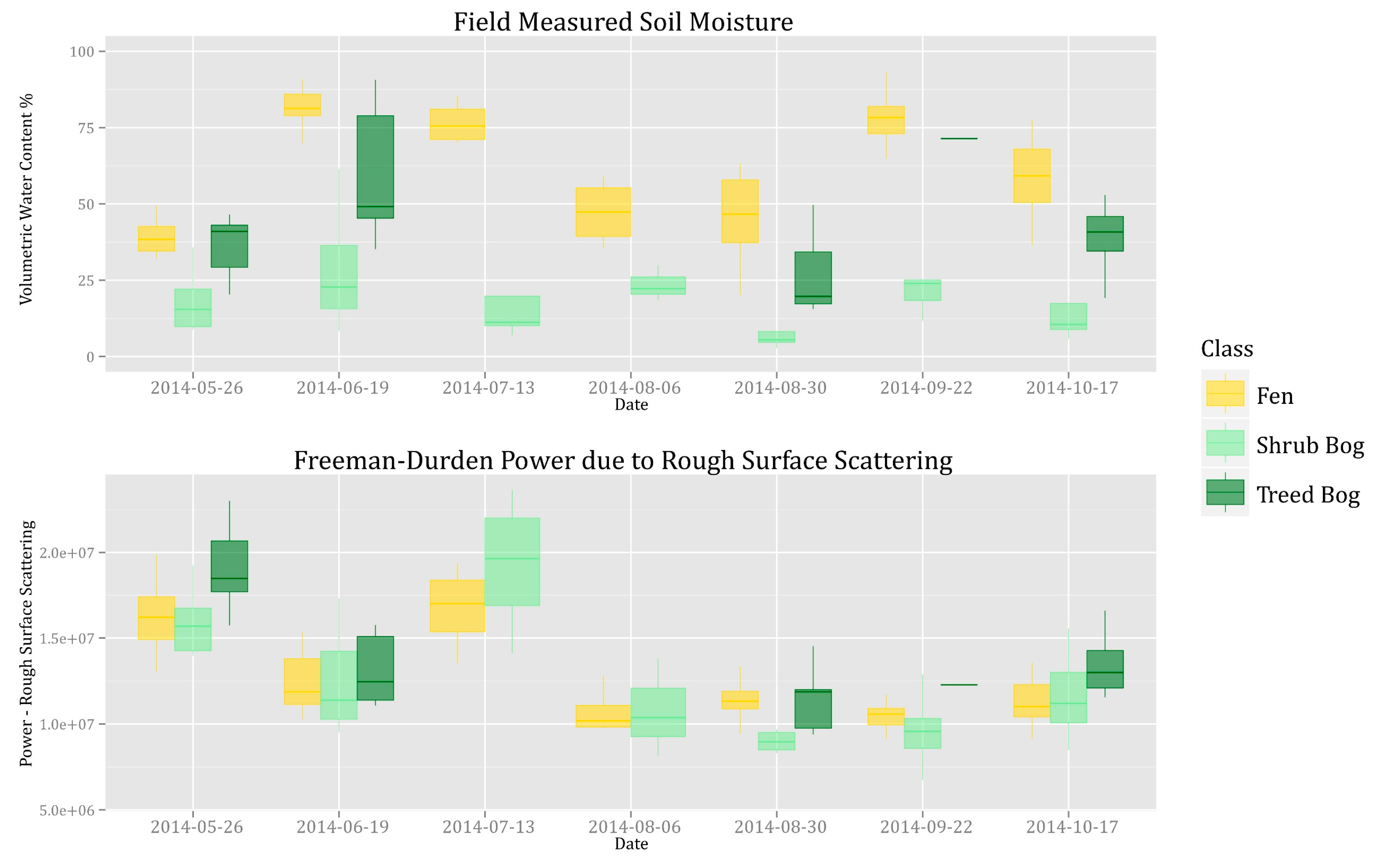
Figure 3.
(Top) Boxplots of field-measured volumetric water content as measured in 2014, grouped by peatland class and date; (Bottom) Boxplots of Freeman-Durden Power due to Rough Surface Scattering (SAR decomposition parameter) extracted at field measurement sites in 2014, grouped by peatland Class and Date.

Figure 4.
Examples of predicted volumetric water content (VWC) for 30 August 2014 based on three different Mixed Effects models. The Legend for the overview map follows Figure 2. We chose to display the results of the 30 August as, in single-date models published in previous research [20], this date resulted in the highest model explained variance (R2 = 0.47) but the lowest independently validated explained variance (R2 = 0.1) but was the highest independently validated single-date model in [20].


Table 1.
List of remote sensing image acquisition dates. Measurements of field data coincide with SAR data acquisition dates. For full soil moisture acquisitions, n = 32. For partial acquisitions, the sample size on that date is in brackets in the SAR Data column.
Table 1.
List of remote sensing image acquisition dates. Measurements of field data coincide with SAR data acquisition dates. For full soil moisture acquisitions, n = 32. For partial acquisitions, the sample size on that date is in brackets in the SAR Data column.
| SAR Data (FQW1 ASC) | MODIS NDVI Composite | Lidar Data | ||
|---|---|---|---|---|
| Field Data Collection | Partial Soil moisture | 13 July (8) | 11 July–28 July | 11 May |
| 6 August (7) 22 September (15) | 28 July–13 August 13 September–29 September | |||
| Full soil moisture | 26 May | 24 May–10 June | ||
| 19 June 30 August | 10 June–26 June 29 August–13 September | |||
| 17 October | 15 October–4 November |
Table 2.
Model results including the method of validation, R2 (marginal, conditional, model, independently validated) and RMSE (model and independently validated). Model A (Random Sample) was run 10 times with a bootstrapped random sample of 50 data points to provide a cross validation and is not a truly independent validation*. Each independent validation was completed by leaving out one site/date for each model run. Validated root mean square error (RMSE) and R2 are based on the average of validation of all withheld dates/sites. Environment variables-only model represents a model with no remotely sensed data (landscape-level covariates). Marginal R2 represents the fixed effects component of the model and conditional R2 represents both fixed and random, calculated using piecewiseSEM [45]. A linear (non-mixed effects) model using only SAR as a predictor was run for comparison.
| Validated By | Marginal R2 | Conditional R2 | Model RMSE | Model R2 | Indep. Validated RMSE | Indep. Validated R2 | |
|---|---|---|---|---|---|---|---|
| (Environment Variables-Only) VWC~Drought Code + Day of Year + and Number of Days Since Last Rain + (1|date) | Site | 0.16 | 0.6 | 12.2 | 0.70 | 38.0 | <0 |
| (Linear SAR only) VWC~FDPRS | Date | NA | NA | 33.1 | 0.18 | 49.2 | <0 |
| (A) VWC~FDPRS + (1|date) + (1|Class:Site) | Random Sample | 0.02 | 0.78 | 10.4 | 0.88 | 12.2 | 0.74 * |
| (B) VWC~FDPRS + (1|Class:Site) | date | 0.07 | 0.23 | 31.8 | 0.24 | 34.8 | 0.13 |
| (C) VWC~FDPRS + (1|date) + (1|Class) | Site | 0.01 | 0.75 | 13.8 | 0.71 | 14.5 | <0 |
| (D) VWC~FDPRS + (1|date) | Site | 0.14 | 0.43 | 20.1 | 0.39 | 19.5 | <0 |
| (E) VWC~FDPRS + (1|Class) | Date | 0.07 | 0.50 | 18.5 | 0.44 | 20.0 | 0.30 |
| (F) VWC~FDPRS + (1|Site) | Date | 0.03 | 0.54 | 15.2 | 0.63 | 18.9 | 0.22 |
| (G) VWC~FDPRS + LiDARveg + MODIS + (1|Class) | Date | 0.39 | 0.82 | 11.2 | 0.88 | 23.2 | 0.22 |
| (H) VWC~FDPRS + LiDARveg + MODIS + Drought Code + Day of Year + Number of Days Since Last Rain + (1|Class) | Date | 0.51 | 0.80 | 11.7 | 0.89 | 36.8 | <0 |
| (I) VWC~FDPRS + Drought Code + Day of Year + Number of Days Since Last Rain + (1|Class) | Date | 0.16 | 0.70 | 15.4 | 0.63 | 34.5 | <0 |
| (J) VWC~LiDARveg + MODIS + (1|Class) | Date | 0.14 | 0.64 | 16.1 | 0.61 | 33.1 | <0 |
© 2018 by the authors. Licensee MDPI, Basel, Switzerland. This article is an open access article distributed under the terms and conditions of the Creative Commons Attribution (CC BY) license (http://creativecommons.org/licenses/by/4.0/).
Share and Cite
MDPI and ACS Style
Millard, K.; Thompson, D.K.; Parisien, M.-A.; Richardson, M. Soil Moisture Monitoring in a Temperate Peatland Using Multi-Sensor Remote Sensing and Linear Mixed Effects. Remote Sens. 2018, 10, 903. https://doi.org/10.3390/rs10060903
AMA Style
Millard K, Thompson DK, Parisien M-A, Richardson M. Soil Moisture Monitoring in a Temperate Peatland Using Multi-Sensor Remote Sensing and Linear Mixed Effects. Remote Sensing. 2018; 10(6):903. https://doi.org/10.3390/rs10060903
Chicago/Turabian StyleMillard, Koreen, Dan K. Thompson, Marc-André Parisien, and Murray Richardson. 2018. "Soil Moisture Monitoring in a Temperate Peatland Using Multi-Sensor Remote Sensing and Linear Mixed Effects" Remote Sensing 10, no. 6: 903. https://doi.org/10.3390/rs10060903
Note that from the first issue of 2016, this journal uses article numbers instead of page numbers. See further details here.