Developing an Integrated Remote Sensing Based Biodiversity Index for Predicting Animal Species Richness


1
State Key Laboratory of Remote Sensing Science, Faculty of Geography Science, Beijing Normal University, Beijing 100875, China
2
Department of Geographical Sciences, University of Maryland, College Park, MD 20742, USA
*
Author to whom correspondence should be addressed.
Remote Sens. 2018, 10(5), 739; https://doi.org/10.3390/rs10050739
Submission received: 2 March 2018
/
Revised: 24 April 2018
/
Accepted: 5 May 2018
/
Published: 10 May 2018
(This article belongs to the Special Issue Advances in Quantitative Remote Sensing in China – In Memory of Prof. Xiaowen Li)
Abstract
:Many remote sensing metrics have been applied in large-scale animal species monitoring and conservation. However, the capabilities of these metrics have not been well compared and assessed. In this study, we investigated the correlation of 21 remote sensing metrics in three categories with the global species richness of three different animal classes using several statistical methods. As a result, we developed a new index by integrating several highly correlated metrics. Of the 21 remote sensing metrics analyzed, evapotranspiration (ET) had the greatest impact on species richness on a global scale (explained variance: 52%). The metrics with a high explained variance on the global scale were mainly in the energy/productivity category. The metrics in the texture category exhibited higher correlation with species richness at regional scales. We found that radiance and temperature had a larger impact on the distribution of bird richness, compared to their impacts on the distributions of both amphibians and mammals. Three machine learning models (i.e., support vector machine, random forests, and neural networks) were evaluated for metric integration, and the random forest model showed the best performance. Our newly developed index exhibited a 0.7 explained variance for the three animal classes’ species richness on a global scale, with an explained variance that was 20% higher than any of the univariate metrics.
1. Introduction
Changes and losses in global biodiversity have been rapidly accelerating in recent years [1,2,3,4,5,6]. Understanding of both current patterns and change tendency is a key concern for scientists, ecologists, and policy-makers. Biodiversity has a multitude of facets that can be quantified, and the most commonly considered one is species richness [7,8]. Species richness is the number of species in a site, habitat, or clade [1,9]. Much research has focused on the distribution of animal species richness [10,11,12,13,14,15]. In addition, a growing amount of data infrastructure has been constructed for continental-to-global scale species monitoring and analysis [16,17]. The Global Biodiversity Information Facility (GBIF) and the International Union for Conservation of Nature (IUCN) provides access to millions of current global digitized species records [18,19,20]. However, the scale limitation of in situ data has hindered large-scale species monitoring. The collection of in situ data is too costly to be applied in long time-series species monitoring.
Remote sensing is a powerful tool in global biodiversity assessment because it enables consistent observations of species across time and space, as well as the tracking of climatic change and other drivers of species change [4]. Based on remote sensing technology, two common methods are used for the observation of species richness: direct species monitoring and indirect species monitoring. In direct species monitoring, the high spatial and spectral resolution of remote sensing data enables individual species to be distinguished from nearby pixels, and the associations of single species can be evaluated based on the individual species [21,22]. However, this method requires extremely high spatial and spectral resolution remote sensing data, which are generally not available to the general public. Considering the distribution differences between different species or classes, a comprehensive biodiversity assessment on a global scale is too costly to achieve by using direct species monitoring [10,11,23,24]. To increase the monitoring scale and evaluate more species or classes, indirect species monitoring mainly maps the key environmental factors which relate to species distribution using remote sensing data [25,26]. Compared with direct species monitoring, indirect species monitoring shows less requirement for high spatial and spectral resolution of remote sensing data, and can thus facilitate continuous large-scale species monitoring.
Previous studies have found that a variety of factors impact the distribution of animal species, mainly in four categories: energy/productivity [27,28,29]; climate [11,30,31,32]; ecosystem texture [33,34]; and evolutionary history [24]. Energy/productivity, climate, and ecosystem texture can be continuously monitored using remote sensing data. The species-energy hypothesis predicts that more species and higher abundances of individual species will occur where more energy in the form of food is consistently available [35,36,37,38]. Climate change can lead to systematic changes of species distribution [39,40]. Ecosystem texture determines the physical structure of the environment, and therefore, has a considerable influence on the distributions and interactions of animal species [41,42,43]. Based on these theories and hypotheses, recent studies have developed several frameworks, such as Essential Biodiversity Variables (EBVs) and Remote Sensing Essential Biodiversity Variables (RS-EBVs), which have been used to construct a global species-observing system [2,44]. Meanwhile, many new remote sensing metrics have been developed to monitor species on a global scale [25,26,45,46,47,48]. The most outstanding feature of these metrics is that they can be generated on a global scale. Assessment of different remote sensing metrics on a global scale and the development of a multivariate integration index is essential for global biodiversity assessment, but such efforts are missing from the literature. Available larger-scale species richness datasets offer a valuable database for the assessment of these remote sensing metrics. Instituto de Pesquisas Ecológicas (Brasil) offers a suite of large-scale species richness data [49], which has been validated in previous studies and exhibits high accuracy [50,51].
Machine learning provides a great opportunity for the study of species richness, while construction of mechanistic models between species richness and remote sensing metrics is still challenging [52,53]. Compared with traditional mechanistic approaches, machine learning avoids the over-simplification during modelling. Machine learning models are as complex as real ecosystems, therefore, in most cases the results that come from machine learning are more valid for drawing any conclusions for real situations [54,55]. Moreover, machine learning has been widely used for species assessment and prediction [56,57,58].
In this study, to assess remote sensing metrics on a global scale, we selected in situ species richness data on three animal classes (mammals, birds, and amphibians) and 21 remote sensing metrics that all had global coverage and long-term availability (Table 1). We analyzed the correlations between animal species richness and remote sensing metrics, and developed a multivariate integration index based on a machine learning model. This study aimed to address the following questions:
- (1)
- What are the differences between the distributions of various animal classes (mammals, birds, and amphibians) on a global scale?
- (2)
- What are the correlations between remote sensing metrics and species richness distributions on a global scale?
- (3)
- Given the major driving metrics, can we develop a multivariate integration index to map the global species richness continuously?
2. Data and Methods
2.1. Data
2.1.1. Species Richness Data
Considering coverage and taxonomy, we chose to use the species richness dataset from the Instituto de Pesquisas Ecológicas (Brasil) in this study. This dataset (grid format) consists of global total mammal richness, global total bird richness, and global total amphibian richness. In this dataset, the primary species range map data used to create the species richness maps are from the IUCN for mammal and amphibian species, and jointly from BirdLife International and NatureServe for bird species. During the data process, extinct species were removed, as were non-native distributions of extant species. For each grid cell, any species that overlapped any part of the cell were counted as a presence of that species. All species richness data exhibited a spatial resolution of 10 km and used the equal-area projection [3,49,50,59].
2.1.2. Remote Sensing Data
Considering the availability of datasets, three categories of remote sensing metrics were collected: energy/productivity metrics, climate metrics, and ecosystem texture metrics. Because the species richness data was recorded and updated for decades, we selected the remote sensing data as long-term as possible. In addition, all remote sensing data had global coverage.
For the energy/productivity category, we selected gross primary production (GPP), dynamic habitat index (DHI), and potential evapotranspiration (PET). The GPP product was obtained from the global monthly MOD17A2 GPP product [60]. The DHI, including Cumulative Annual Productivity (DHI-cum), Minimum Annual Apparent Cover (DHI-min), and Seasonal Variation of Greenness (DHI-sea), is a composite vector deduced from the Fraction of Absorbed Photosynthetically Active Radiation (FAPAR) time-series, representing the vegetation dynamics. The monthly maximum FAPAR-value is the basic input dataset to compute the three relevant annual indices for the subsequent habitat analysis [51,61]. DHI-cum provides an indication of overall site vegetation productivity. DHI-min represents the lowest (minimum value) level of vegetative productivity in a year. DHI-sea refers to the variation of the vegetative productivity. Further details of the DHI can be found in previous publications [51,61,62,63]. In this study, DHI was calculated from the Global Inventory Modelling and Mapping Studies (GIMMS) AVHRR-FAPAR 3g dataset. The PET product was obtained from the MOD16A2 product. In our study, PET was taken as an energy/productivity metric, because it characterizes the features of the surface temperature and radiance.
For the climate category, we selected evapotranspiration (ET) and land surface temperature (LST). The ET product was obtained from the global monthly MOD16A2 ET product [64,65,66,67,68]. The LST product used in this study was obtained from the global monthly MOD11C3 LST product, which belonged to the temperature/surface emissivity global data sets (C5) [69].
For the texture category, we selected a suite of global terrestrial habitat heterogeneity data, which was developed by Haralick et al. and computed by Tuanmu and Jetz using the Moderate Resolution Imaging Spectroradiometer (MODIS) Enhanced Vegetation Index (EVI) product [25,70]. Heterogeneity is an important indicator of ecosystem texture, which has long been recognized as a key landscape characteristic with strong relevance for biodiversity [71,72]. These heterogeneity metrics consist of the coefficient of variation (CV), evenness, contrast (CON), dissimilarity (DIS), entropy (ENT), homogeneity (HOM), range, Shannon, Simpson, standard deviation (SD), correlation (COR), maximum (MAX), uniformity (UNI), and variance (VAR).
2.1.3. Biome Data
Biome data acquired from World Wildlife Fund (WWF) were used for this study. This data depicted the 14 terrestrial biomes of the globe, which include eight forest biomes, four grassland biomes, one tundra biome, and one desert biome [73]. Biomes are relatively large units of land containing distinct assemblages of natural communities and species, with boundaries that approximate the original extent of natural communities prior to major land-use change [74]. This comprehensive, global data provide a useful tool for identifying areas of outstanding biodiversity and conservation priority.
2.2. Methods
The overall procedure for the proposed method is briefly illustrated in Figure 1. Comparison of the remote sensing metrics and development of the multivariate integration index were achieved through four tasks.
2.2.1. Data Integration and Standardization
In data integration, to enable all data to have the same resolution, long time-series LST, ET, GPP, PET, DHI-cum, DHI-min, and DHI-sea data were averaged on time-scales. Mammal richness, bird richness, and amphibian richness were added together to generate a variate “Allclasses” as the surrogate for all three animal classes.
In data standardization, remote sensing metrics were normalized (0–1) using the feature scaling method, because absolute values had large differences in magnitude. All species richness data and remote sensing metrics were summed to a 0.1° spatial resolution separately using the nearest-neighbor interpolation method, because the lowest spatial resolution of the datasets was 10 km (species richness data). In order to remove the impact of non-value area, we excluded the areas which had non-value pixels of species richness data or remote sensing metrics.
2.2.2. Regression Analysis
Before the regression, we used the function randomu in Interface Description Language (IDL) to extract 10,000 pixels randomly from the global terrestrial areas of species richness data and each remote sensing metric. The univariate linear regression model was used to evaluate the correlation of these metrics with animal species richness. Since the relationships between species richness and some metrics were nonlinear, we used locally weighted regression (LOESS) to determine the pattern of relationships [75,76]. We took a logarithmic transform for COR, CV, and DHI-sea, and used polynomial regression for evenness, CON, DIS, ENT, HOM, range, Shannon, Simpson, SD, MAX, UNI, VAR, LST, ET, GPP, and PET.
2.2.3. The Akaike Information Criterion
The Akaike information criterion (AIC) was used to evaluate the model quality. The AIC is a measure of the quality of each model, relative to each of the other models for a given set of data [77,78,79], and the AIC value of the model can be expressed as:
where L is the maximum value of the likelihood function for the model, and c is the number of free parameters in the model. The model with the smallest AIC is the best performance. Thus, the good performance of different models in this study was normally based on the low AIC values.
2.2.4. Three Machine Learning Methods for Metrics Integration
After determining the relationships between each remote sensing metric and species richness, we selected the high-explained-variance metrics to develop a multivariate integration index using machine learning models. In this study, we compared the capability of support vector machine (SVM), random forests (RF), and neural networks (NN) to integrate various metrics. Species richness was trained on 50% of the randomly extracted pixels and cross-validated on the remaining 50%. The same number of pixels was used for training and predicting in order to avoid under- or over-fitting due to an unbalanced dataset [80].
Support vector machine (SVM) is a supervised machine learning model with associated learning algorithms that analyze data used for classification and regression analysis [81]. SVM uses kernel functions implicitly to map training data into a higher-dimensional feature space. The maximum separation hyperplane is defined by a set of support vectors, which are a function of the training data that lie on/the closest to the separating margin [82]. In this study, the e1071 library of the R statistical package was utilized to optimize the SVM parameters [83].
Random forests (RF) is a regression model that grows an ensemble of trees [84,85]. Each tree casts a unit vote for the most popular class according to the input variables. The growing process of RF is by bootstrap aggregating (or bagging), where a tree is randomly grown from the dataset, and this process can provide substantial gains in the accuracy of predicting models [86,87], and it requires no pruning. In this study, we used the RF algorithm implemented in the randomForest R package, with the parameter values for the algorithm, (i.e., number of trees to grow (ntree)) equaled to 500, and the number of descriptors randomly sampled at each split (mtry) equaled to the total number of descriptors in the dataset divided by three.
Neural networks (NN) is a non-linear statistical data modelling tool used for prediction and regression. We selected the multilayer feed-forward neural network, which is one of the most popular approaches to neural networks (NNs) [88,89,90]. The multilayer feed-forward NN is a backpropagation network that trains the data using a backpropagation algorithm [84,91]. This network comprises three layers: an input layer, one or more hidden layers, and an output layer. Neurons from one layer are in one direction linked to all neurons in the subsequent layers [92]. This study used the nnet library provided by the R package in order to develop the model [36]. The nnet package is the library for establishing multiple feed-forward NNs with more than one hidden layer [93]. This study constructed the model by carrying out the learning for a total of 30 times with the maximum number of iterations at 100.
3. Results
3.1. Richness Distribution of Three Animal Classes
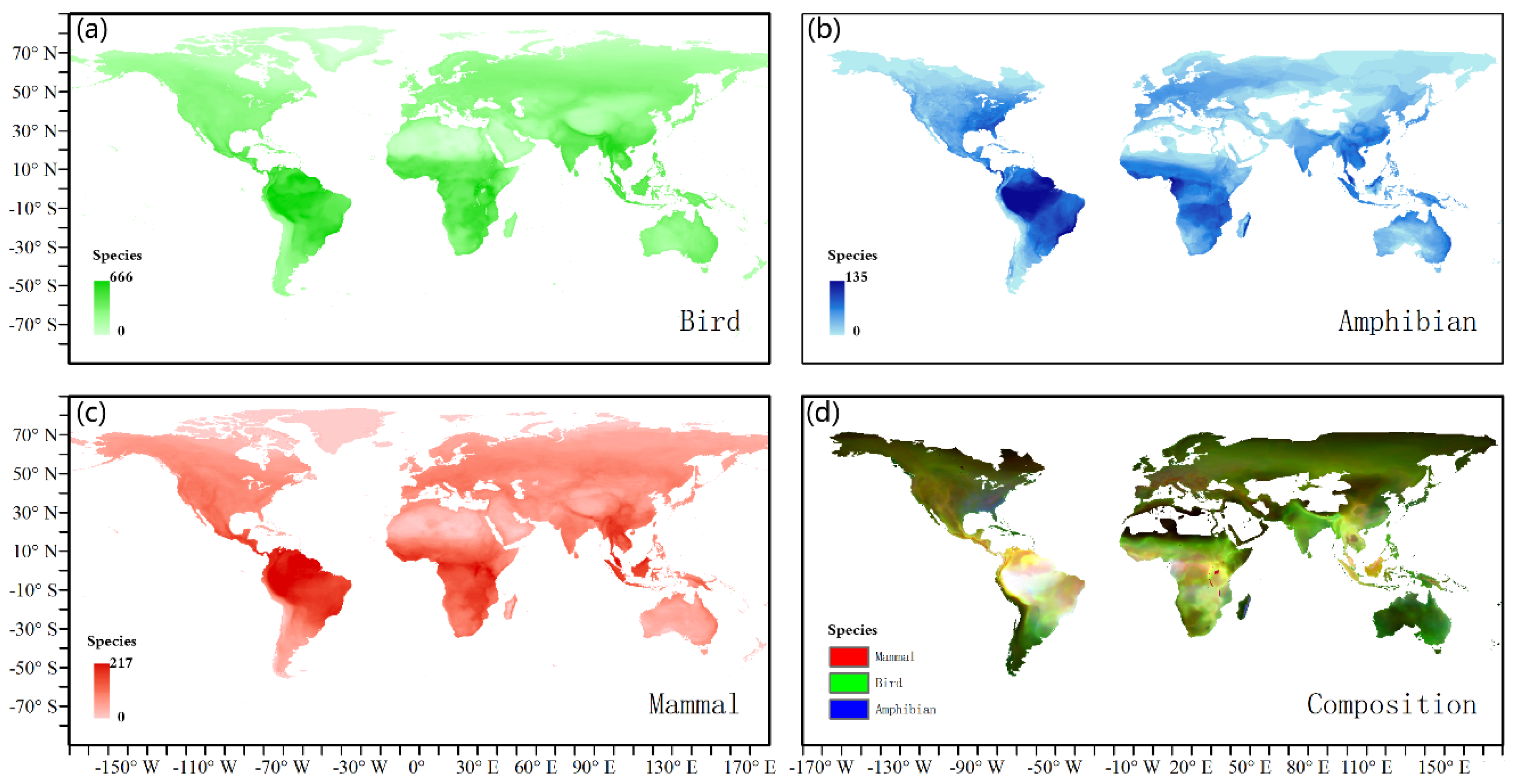
The distribution of mammal, bird, and amphibian species richness (normalized) was mapped on a global scale. Mammals, birds, and amphibians showed similar distribution patterns at low latitudes (Figure 2). In the Amazon, the species richness patterns of mammals, birds, and amphibians were almost equal. Distribution differences between mammals, birds, and amphibians were observed at mid–high latitudes. The species richness of birds and mammals was slightly higher than that of amphibians in both Central Africa and Southeast Asia. Overall, the distribution patterns of species richness for these three animal classes were not the same.
3.2. Characterization of Various Remote Sensing Metrics
The scatter plots of various metrics versus species richness showed that most metrics exhibited nonlinear relationships with species richness, and one metric possessed the same type of relationship with various animal classes (Figure S1). DHI-cum and DHI-min showed clear linear positive correlations with species richness. Among the metrics which exhibited nonlinear relationships with species richness, COR, CV, and DHI-sea followed power laws, while the other metrics showed mildly or strongly unimodal relationships (Figure S2).
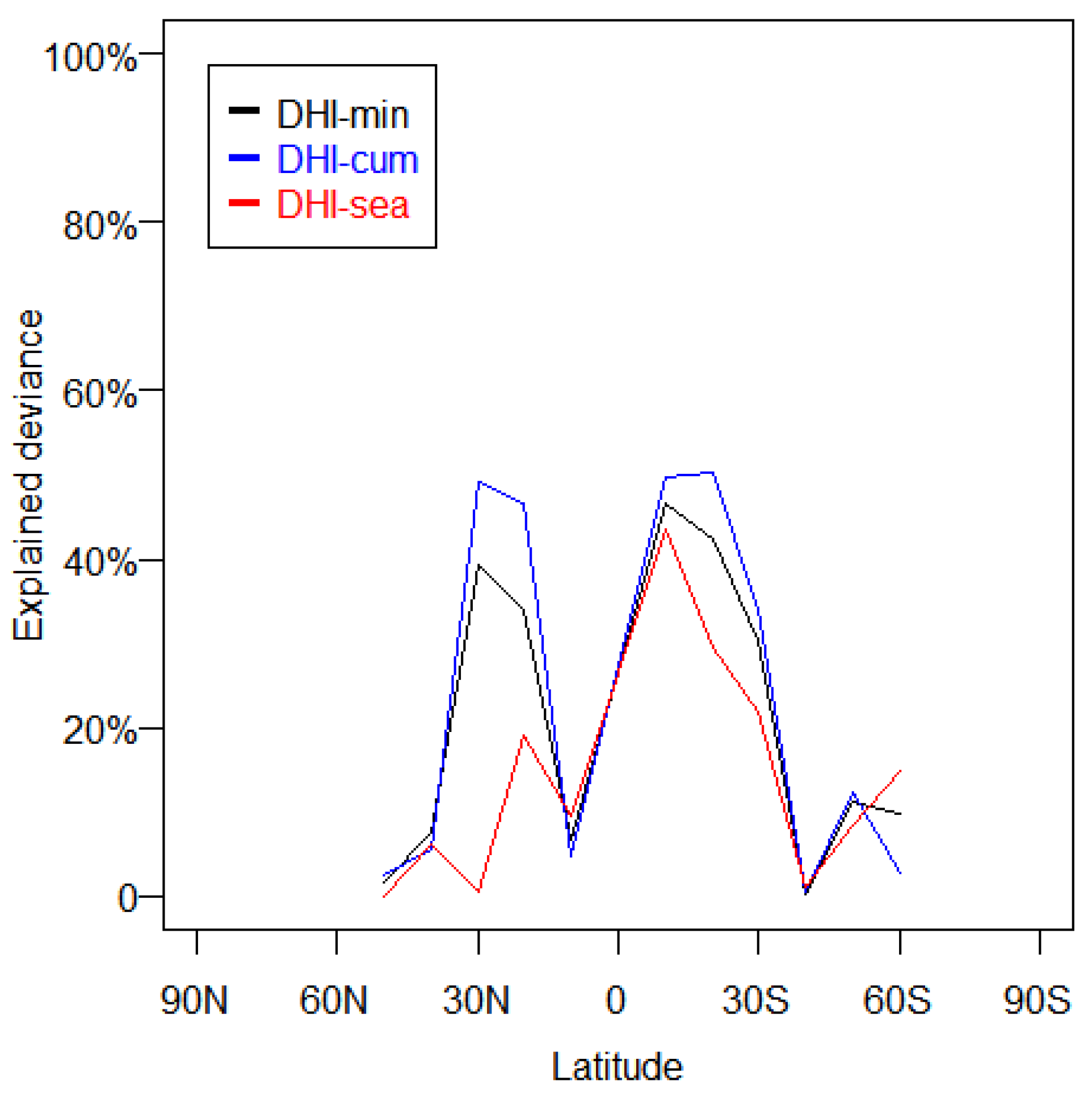
DHI-min, DHI-cum, ET, and GPP exhibited more than 40% explained variance with the distribution of the sum richness of three animal classes on a global scale (Figure 3). These metrics with high explained variance were mainly in the energy/productivity category and the climate category, while the texture category showed weak explanatory power with the distribution of sum richness on a global scale. Among the metrics in the energy/productivity category, DHI-min explained 50% of the sum richness distribution, GPP explained 48%, and DHI-cum explained 46%. DHI-sea exhibited lower than 10% explained variance of DHI-min. The low explained variance of DHI-sea in the southern hemisphere drew down its explained variance on a global scale (Figure 4). For DHI, we detected three dramatic declines of explained variance in 40°N zones, 10°S zones, and 40°S zones (Figure 5). In climate category, ET explained 51% of the sum richness of the three animal classes global distribution, and LST explained 16%. We further observed a large data gap between PET and ET, and PET exhibited lower than 40% explained variance of ET, which indicated that vegetation played an important role in the distribution of animal species richness. The vegetation contributed less to the PET calculation compared to the ET calculation, which might be the primary cause of the difference between PET and ET in the explanation of species richness. Compared with the metrics in the energy/productivity and the climate categories, almost all texture metrics showed low explained variance. Among the texture category, CV exhibited the highest explained variance (22%), while COR and evenness showed negligible explained variance.
Some differences were observed when we examined the relationship between remote sensing metrics and individual animal class (Figure 3). Compared with mammals and amphibians, birds exhibited higher explained variance with PET, and exhibited lower explained variance with ET. Birds showed lower sensitivity than amphibians and mammals to the energy/productivity category metrics (e.g., GPP, DHI-sea, DHI-min, and DHI-cum). Mammals were more sensitive to ET, with an explained variance that was 6% higher than that of birds and amphibians. For ENT and HOM, the explained variance of amphibians was lower than that of mammals and birds.
3.3. Integration of Various Remote Sensing Metrics
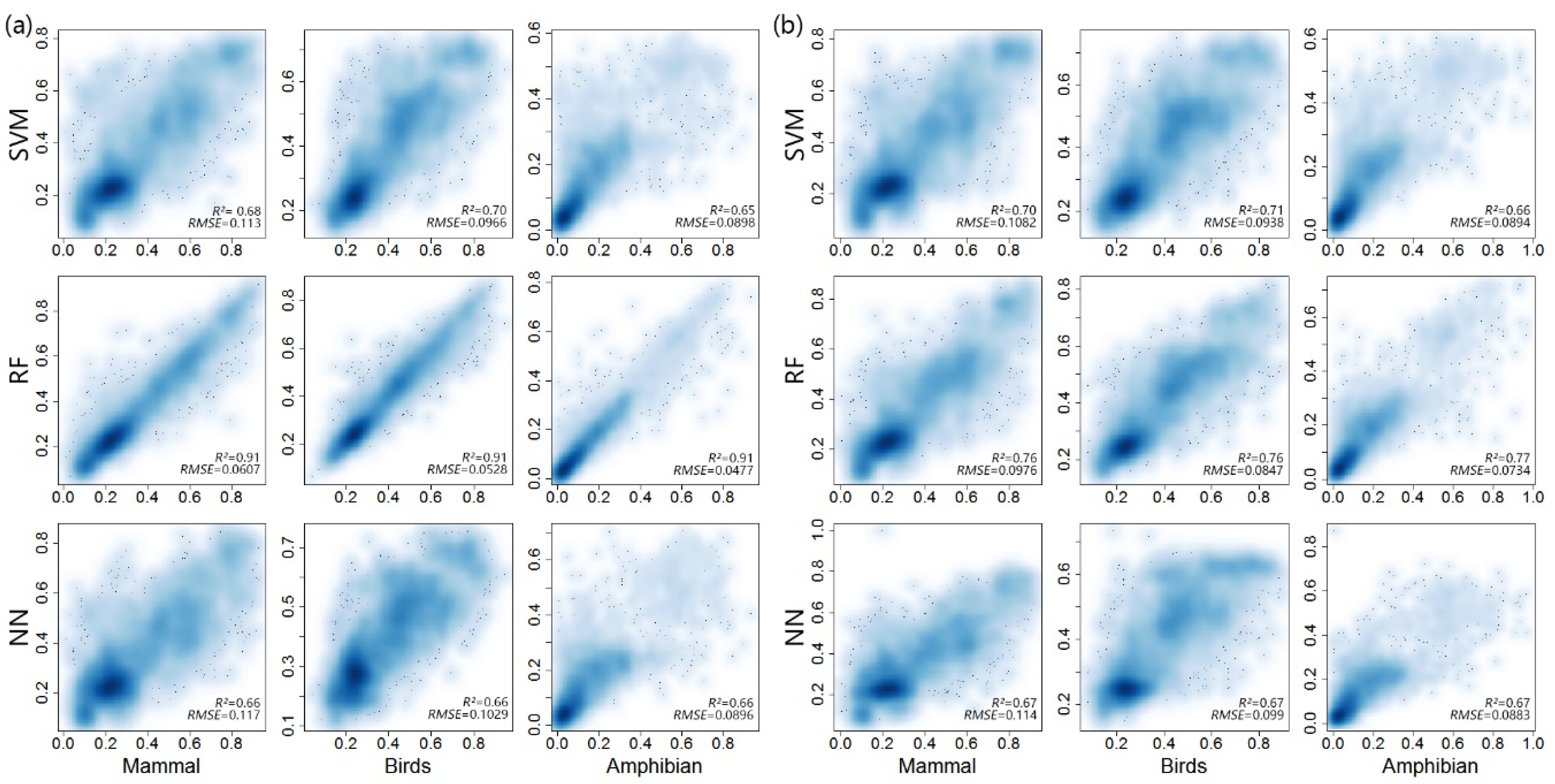
Based on the characterization of various metrics and AIC values, DHI-min, DHI-cum, DHI-sea, GPP, CV, ET, and LST were selected as the major metrics for the development of an integrated biodiversity index. For the AIC values, the RF model gave the lowest AIC for species richness of the three animal classes when compared to SVM and NN (Figure 6). The species richness data of each animal class predicted by the same machine learning model were quite similar, and RF exhibited a higher r-square value than SVM and NN in species richness of all three animal classes (Figure 7). The r-square values of mammals, birds, and amphibians were 0.76, 0.76, 0.77, respectively, according to the RF model; 0.7, 0.71, and 0.66, respectively, according to the SVM model; and 0.67, 0.67, and 0.67, respectively, according to the NN model. In terms of the root mean squared error (RMSE), the prediction of the RF model exhibited a lower RMSE than the other two models for all three animal classes. Overall, the RF model outperformed the other two models for species richness prediction. We used the RF model to integrate the seven metrics and develop a multivariate integration index.
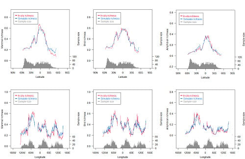
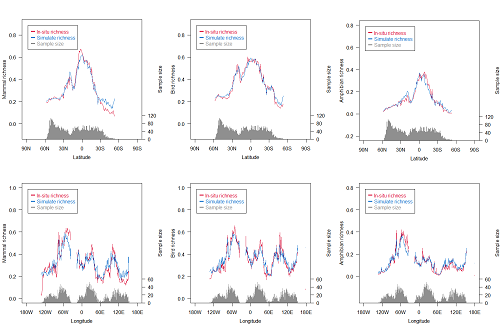
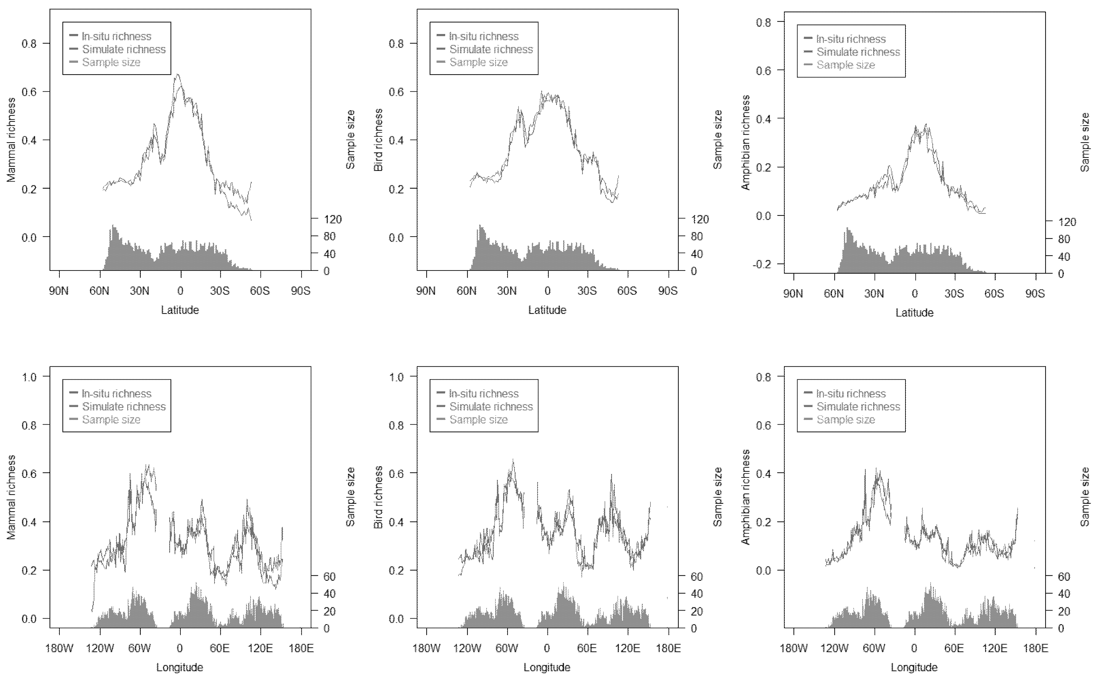
The multivariate integration index exhibited a higher explained variance than the univariate metrics, and exhibited more than 76% explained variance for the species richness of the three animal classes on a global scale. For a single animal class, the gap between the multivariate integration index and the univariate metrics was more than 30% (Figure 3 and Figure 7). On the whole, the simulated species richness showed a consistent spatial pattern with in situ richness (Figure 8). At regional scales, the simulated species richness was in good agreement with in situ species richness in most regions. However, the differences between simulated species richness and in situ species richness were observed. For mammals, simulated species richness was higher than in situ species richness in 40°–60°S zones and 120°–140°E, and simulated species richness was lower than in situ species richness in 0°–10°N and 30°–60°W. For amphibians, simulated species richness was lower than in situ species richness in 30°–60°W. Although disagreements between simulated species richness and in situ species richness were found in some regions, the differences were relatively small in magnitude.
4. Discussion
4.1. Differences in Distribution of the Three Animal Classes
Previous studies have found large mismatches between the priorities of biodiversity protection and protected lands in the United States, even though many biodiversity protected areas have been established since biodiversity loss was identified [6,50,94,95]. Beside the lack of biodiversity in situ datasets, this mismatch has likely arisen from differences in the distribution of various animal classes. Protected areas are generally established for the protection of specific species, while biodiversity includes many different taxa. In the United States, mammal richness was found to be very high in the west, and bird richness was high in coastal regions [49,50]. A similar result was also found in our comparison, in which we examined the distribution of mammals, birds, and amphibians, based on the latest global in situ data. In addition, the differences in the distribution of mammals, birds, and amphibians were mainly observed at mid–high latitudes. This is probably because the limitation of water or energy/productivity at mid–high latitudes leads the difference in species richness among the three animal classes [96]. In this study, biodiversity metrics did not exhibit a large gap in explained variance between various animal classes, although the global distribution of various animal classes were different. This may be due to the offset of regional differences, which led to a similar statistical result on a global scale.
4.2. Attribution of Differences between Remote Sensing Metrics
For energy/productivity category, a large number of studies have attempted to discover the relationship between energy/productivity and species richness in past decades [29,97,98]. The species-energy theory proposes that the supply of useable energy in the environment is very important to species richness [96,99]. Although this theory is based on studies which are mainly focused on the richness of plant species, for animals, there is a less dramatic shift in the relationship between productivity and species richness [100]. Animal richness is limited primarily by the production of plants at the base of the global food web [35,99]. That is probably the reason that the high explained variance metrics were mainly found in the energy/productivity category among the remote sensing metrics in this study. The relationship between energy/productivity metrics and the richness of animal species exhibits several patterns, namely linear pattern, unimodal pattern, exponential pattern, or no pattern at all [100,101,102]. Past researchers also found this relationship differs in different scales [100]. Our study showed, on a global scale, that DHI-min and DHI-cum exhibited a linear relationship with richness of the three animal classes; DHI-sea exhibited an exponential relationship with richness of the three animal classes; and GPP exhibited an unimodal relationship with richness of the three animal classes. In our study, DHI-sea exhibited a low explained variance of 38.9%, which was different to DHI-min and DHI-cum. Species richness may be reduced through a decrease in either cumulative annual productivity or minimum annual productivity. However, the impact of DHI-sea on species richness can be different to the impacts of DHI-min and DHI-cum. The influence of annual variation on productivity will be limited when the cumulative annual productivity or minimum annual productivity is constant. Since the impact of short-term low productivity can be offset by subsequent high productivity, it has a less immediate impact than DHI-min and DHI-cum. That is probably why we observed a smaller impact of DHI-sea. Overall, DHI-min, DHI-cum, and GPP should be selected as main factors for predicting animal species richness on a global scale.
For climate category, past investigations showed that global patterns of species richness were widely correlated with climate [24,103]. Climate change can influence the animal distribution directly by itself, and also affects animal species richness through changing vegetation productivity. In this study, we evaluated the impacts of LST and ET on animal species richness. ET exhibited the highest explained variance among all remote sensing metrics, which indicated the great impact of the water component on species distribution. Moreover, the difference of explained variance between ET and PET indicated that vegetation productivity played an important role in the distribution of animal species richness, because vegetation contributed less to the PET calculation compared to the ET calculation. The explained variance of LST was lower than ET, DHI-min, DHI-cum, and GPP. This may be due to the time-lag effects in the response of species richness to climate change. Previous studies showed that the change in animal diversity lagged behind climate change [39]. Some research has revealed that a warmer winter will lead animal diversity to change by causing the long-distance migration of animals [40]. Moreover, climate can alter species richness distribution through changing the vegetation productivity [104], and many studies have found a time-lag in the global vegetation response to climate change [105,106,107,108]. Because the influence of climate factors on animal diversity varies with different regions which leads to an offset on global-scale analysis, we expect that explained variance of LST are higher in regional analysis.
For the ecosystem texture category, texture metrics have been proved to be important drivers of animal species richness [11,25,48,71,72,109], but the relationship pattern of texture metrics with animal species richness is still controversial. Various studies have found that species richness exhibited positive relationships with environmental heterogeneity, while negative relationships between environmental heterogeneity and species richness have also been reported [27,43,110,111,112,113]. Tuanmu and Jetz [25] validated the performance of 14 heterogeneity metrics, using North American bird richness. They showed that the texture metrics combined with net primary productivity (NPP) can explain up to 35.8% of the variance. In addition, homogeneity could still explain about 8% of the variance by itself. In the ecosystem texture category, our results showed that the CV was the strongest metric on a global scale, with an explained variance of 22%. Compared with metrics in energy/productivity and climate category, this study showed that texture metrics exhibited low explained variance on a global scale, while high correlations were observed at smaller scales. In fact, the pattern of the relationship between animal species richness and habitat heterogeneity was impacted by many factors. Previous studies have showed that the possible effects of heterogeneity may also vary relative to the structural variable measured, and the effect of habitat heterogeneity for one species group may differ in relation to the spatial scale [43,71]. In this study, the high-correlation areas were mainly covered shrub lands, grasslands, and savannas, while the explained variance of texture metrics were relatively low in forests (Table S1). This is probably because the texture dataset we used mainly focused on the horizontal structure of an ecosystem, while forest biome has more complex vertical structures than shrub lands, grasslands, and savannas. Moreover, different regions showed various major driving texture metrics. For example, DIS, ENT, and HOM exhibited high explained variance in grasslands and savannas. Moreover, previous studies found that the predictive performance of texture metrics would vary across different spatial scales [114]. Overall, texture metrics should be primarily considered when determining the species distribution at regional scales.
For different animal classes, we found a gap in the explained variance between bird species richness and the species richness of the other two animal classes, among the climate metrics. The explained variance of PET on bird richness was much higher than that of both amphibian and mammal richness, which indicated that radiance and temperature played a more important role in bird richness distribution than in the other two animal classes.
4.3. Integration of Various Remote Sensing Metrics
The effect mechanism of different environmental variables on species distribution is debatable [115], which limits the application of certain metrics to model the species distribution quantitatively. We applied three commonly used machine learning models in the integration of the remote sensing metrics. There were differences in the results generated from the three models; RF generally outperformed SVM and NN in our case study. In this study, SVM and NN exhibited high uncertainty in species richness modeling, with the estimated datasets showing higher r-square and lower RMSE than the training datasets. In consideration of the AIC values, the RF model provided a better representation of the metrics integration of remote sensing metrics in this study than the other two models. Previous studies have suggested that differences in the results of various machine learning models may be due to the sample size, or the ratio between the size of the training sample and the estimated sample. [116,117]. However, there was no improvement in the performance of SVM and NN in species richness modeling, when we increased the proportion of the training sample and decreased the proportion of the estimated sample (Figure S3). RF has broader scope than SVM and NN, because it has no limitation on the distribution pattern of the training data. The complexity of the parameter setting may limit the performance of SVM and NN for model training [118]. Although, SVM has the advantage on solving non-linear problems, a major downside of SVM is that it can be painfully inefficient to train [119,120]. Another main advantage of RF is that it handles very well with a large number of training examples, and it is not recommended to use SVM to handle large training examples, which might lead to a better performance of the RF. In the training process, we observed a large gap between RF, SVM, and NN. In addition, the computation time required for modelling differed considerably among the three machine learning models (Table 2). The computational efficiency of the SVM and NN models were much higher than that of the RF model.
In this study, the multivariate integration index based on the RF model exhibited 20% more explained variance than the univariate metrics. Many species richness monitoring and modelling studies have been carried out in previous decades [3,4]. Our result, using three categories of remote sensing metrics, exhibited twice the explained variance of previous studies, which used texture metrics and net primary productivity (NPP) [25]. Previous studies showed DHI components explained between 47% and 75% of total bird species richness (BBS) in Ontario (North America), and we extended the spatial scale from regional to global [61]. Although these studies selected different species richness datasets, a comparison of the correlations was still reasonable, and we asserted that the multivariate integration index had a better correlation with species distribution than univariate metrics on a global scale. Since the evolution of a species is a very slow process, the link between these remote sensing metrics and species characteristics is stable for decades [121]. Thus, the multivariate integration index we developed can be used for mapping the global species richness annually, which would provide great support for global biodiversity trend detection.
At latitudinal and longitudinal zones, some differences between simulated species richness and in situ species richness were observed (Figure 8). There were two possible reasons that led to this disagreement. Firstly, these zones (e.g., 40°–60°S zones) where gaps of species richness were found mostly had large areas of water or deserts, which led to a small sample size for model training. This small sample size brought large uncertainty in simulated species richness. Secondly, in some regions (0°–10°N zones), the limited in situ data constrained much detail of species richness, while the remote sensing metrics we used exhibited high spatial resolution. This difference limited the explained variance of some remote sensing metrics (e.g., DHI-min, DHI-cum, and DHI-sea) (Figure 3 and Figure 7). Overall, the impact of these differences on the multivariate integration index was limited, since these differences were relatively small in magnitude.
4.4. Limitation and Recommendation for Future Research
Although the multivariate integration index showed a consistent pattern with in situ richness data, it faced two known limitations. Firstly, the limited availability of in situ richness data constrained the comparison and integration of remote sensing metrics. Three dramatic declines of DHI’s explained variance in 40°N zones, 10°S zones, and 40°S zones were found. It appeared that the in situ data of mammal richness were insufficient, because of the detail loss in these regions (Figure 5). Once higher resolution species richness data are available, the multivariate integration index should exhibit higher accuracy. Secondly, relationship patterns between energy/productivity, climate and ecosystem texture metrics, and animal diversity were limited by many other factors, namely scale, resolution, latitude, and so on.
Future research will consider both scale and resolution when comparing remote sensing metrics. Because the focus is taking full advantage of long time-series remote sensing data for species monitoring, some important metrics (e.g., precipitation and air temperature) which are not available from remote sensing data globally, were excluded in this study. To make biodiversity monitoring and assessment more globally accurate, future research will consider more datasets from both remote sensing data and model simulation data in integration index development. In addition, with the collection of more species information of both plants and animals, future research will develop the integration index for predicting plant species richness, as well as animal species richness.
5. Conclusions
In this study, 21 remote sensing metrics were assessed to determine their relationships with the richness distribution of three animal classes. The correlation between the species richness of the three animal classes and 21 biodiversity metrics was evaluated based on regression models, and ET exhibited the strongest correlation with the global distribution of the three animal classes. The metrics with high explained variance were mainly in the energy/productivity category. The ecosystem texture category exhibited a higher correlation with species richness at regional scales. For a single class, we found radiance and temperature had a larger impact on the distribution of birds than the other two animal classes. Three commonly used machine learning models were evaluated to determine their capabilities in developing a multivariate integration index, and the RF model was selected as the optimal model for multivariate index integration. Having taken DHI-min, DHI-cum, DHI-sea, GPP, CV, ET, and LST as the major metrics, the multivariate integration index exhibited a 20% higher explained variance of the global distributions of mammal, bird, and amphibian richness, compared to the univariate metrics. However, the in situ biodiversity data were still insufficient. With improvements in the availability of these datasets, further studies can consider more factors and offer higher-accuracy metrics for the assessment of global biodiversity.
Supplementary Materials
Supplementary materials are available online at https://www.mdpi.com/2072-4292/10/5/739/s1. Figure S1: Correlations of all remote sensing metrics; Figure S2: Scatterplots between species richness and power-law metrics; Figure S3: Correlation between predicted species richness and in situ species richness; Table S1: The explained variance of remote sensing metrics in different biomes.
Author Contributions
J.W. and S.L. conceived and designed the experiments; J.W. performed the experiments; J.W. analyzed the data; J.W. and S.L. contributed to the analysis of the results; all of the aforementioned contributed towards writing the manuscript.
Acknowledgments
This work was partially supported by the National Key Research and Development Plan of China (Grant No. 2016YFA0600102) and the Natural National Science Foundation of China (grant No. 41331173).
Conflicts of Interest
The authors declare no conflict of interest.
References
- Gaston, K.J. Global patterns in biodiversity. Nature 2000, 405, 220–227. [Google Scholar] [CrossRef] [PubMed]
- Pereira, H.M.; Ferrier, S.; Walters, M.; Geller, G.; Jongman, R.; Scholes, R.; Bruford, M.W.; Brummitt, N.; Butchart, S.; Cardoso, A. Essential biodiversity variables. Science 2013, 339, 277–278. [Google Scholar] [CrossRef] [PubMed] [Green Version]
- Pimm, S.L.; Jenkins, C.N.; Abell, R.G.; Brooks, T.M.; Gittleman, J.L.; Joppa, L.N.; Raven, P.; Roberts, C.M.; Sexton, J.O. The biodiversity of species and their rates of extinction, distribution, and protection. Science 2014, 344, 1246752. [Google Scholar] [CrossRef] [PubMed]
- Turner, W. Sensing biodiversity. Science 2014, 346, 301–302. [Google Scholar] [CrossRef] [PubMed]
- Newbold, T.; Hudson, L.N.; Hill, S.L.L.; Contu, S.; Lysenko, I.; Senior, R.A.; Boerger, L.; Bennett, D.J.; Choimes, A.; Collen, B.; et al. Global effects of land use on local terrestrial biodiversity. Nature 2015, 520, 45–50. [Google Scholar] [CrossRef] [PubMed] [Green Version]
- Myers, N.; Mittermeier, R.A.; Mittermeier, C.G.; Da Fonseca, G.A.; Kent, J. Biodiversity hotspots for conservation priorities. Nature 2000, 403, 853–858. [Google Scholar] [CrossRef] [PubMed]
- Butchart, S.H.; Walpole, M.; Collen, B.; Van Strien, A.; Scharlemann, J.P.; Almond, R.E.; Baillie, J.E.; Bomhard, B.; Brown, C.; Bruno, J. Global biodiversity: Indicators of recent declines. Science 2010, 328, 1164–1168. [Google Scholar] [CrossRef] [PubMed]
- Noss, R.F. Indicators for monitoring biodiversity: A hierarchical approach. Conserv. Biol. 1990, 4, 355–364. [Google Scholar] [CrossRef]
- Purvis, A.; Hector, A. Getting the measure of biodiversity. Nature 2000, 405, 212–219. [Google Scholar] [CrossRef] [PubMed]
- Jetz, W.; Rahbek, C. Geographic range size and determinants of avian species richness. Science 2002, 297, 1548–1551. [Google Scholar] [CrossRef] [PubMed]
- Kreft, H.; Jetz, W. Global patterns and determinants of vascular plant diversity. Proc. Natl. Acad. Sci. USA 2007, 104, 5925–5930. [Google Scholar] [CrossRef] [PubMed]
- Guenard, B.; Weiser, M.D.; Dunn, R.R. Global models of ant diversity suggest regions where new discoveries are most likely are under disproportionate deforestation threat. Proc. Natl. Acad. Sci. USA 2012, 109, 7368–7373. [Google Scholar] [CrossRef] [PubMed]
- Jenkins, C.N.; Guenard, B.; Diamond, S.E.; Weiser, M.D.; Dunn, R.R. Conservation implications of divergent global patterns of ant and vertebrate diversity. Divers. Distrib. 2013, 19, 1084–1092. [Google Scholar] [CrossRef]
- Costanza, R.; Fisher, B.; Mulder, K.; Liu, S.; Christopher, T. Biodiversity and ecosystem services: A multi-scale empirical study of the relationship between species richness and net primary production. Ecol. Econ. 2007, 61, 478–491. [Google Scholar] [CrossRef]
- Hurlbert, A.H.; Jetz, W. Species richness, hotspots, and the scale dependence of range maps in ecology and conservation. Proc. Natl. Acad. Sci. USA 2007, 104, 13384–13389. [Google Scholar] [CrossRef] [PubMed]
- Pardieck, K.L.; Ziolkowski, D.J., Jr.; Lutmerding, M.; Campbell, K.; Hudson, M.-A.R. North American Breeding Bird Survey Dataset 1966-2013, Version 2016.0; US Geological Survey: Reston, VA, USA; Patuxent Wildlife Research Center: Laurel, MD, USA, 2017; Available online: www.pwrc.usgs.gov/BBS/RawData/ (accessed on 8 May 2018).
- Constable, H.; Guralnick, R.; Wieczorek, J.; Spencer, C.L.; Peterson, A.T. Vertnet: A new model for biodiversity data sharing. PLoS Biol. 2010, 8, e1000309. [Google Scholar] [CrossRef] [PubMed]
- Garciarosello, E.; Guisande, C.; Heine, J.; Pelayovillamil, P.; Manjarreshernandez, A.; Vilas, L.G.; Gonzalezdacosta, J.; Vaamonde, A.; Granadolorencio, C. Using modestr to download, import and clean species distribution records. Methods Ecol. Evol. 2014, 5, 708–713. [Google Scholar] [CrossRef]
- IUCN. The Iucn Red List of Threatened Species. 2017. Available online: http://www.iucnredlist.org/ (accessed on 8 May 2018).
- GBIF. Gbif Data Portal. 2017. Available online: http://www.gbif.org/ (accessed on 8 May 2018).
- Nagendra, H. Using remote sensing to assess biodiversity. Int. J. Remote Sens. 2001, 22, 2377–2400. [Google Scholar] [CrossRef]
- Gougeon, F.A. Comparison of possible multispectral classification schemes for tree crowns individually delineatedon high spatial resolution meis images. Can. J. Remote Sens. 1995, 21, 1–9. [Google Scholar] [CrossRef]
- Kier, G.; Kreft, H.; Lee, T.M.; Jetz, W.; Ibisch, P.L.; Nowicki, C.; Mutke, J.; Barthlott, W. A global assessment of endemism and species richness across island and mainland regions. Proc. Natl. Acad. Sci. USA 2009, 106, 9322–9327. [Google Scholar] [CrossRef] [PubMed]
- Rahbek, C.; Graves, G.R. Multiscale assessment of patterns of avian species richness. Proc. Natl. Acad. Sci. USA 2001, 98, 4534–4539. [Google Scholar] [CrossRef] [PubMed]
- Tuanmu, M.N.; Jetz, W. A global, remote sensing-based characterization of terrestrial habitat heterogeneity for biodiversity and ecosystem modelling. Glob. Ecol. Biogeogr. 2015, 24, 1329–1339. [Google Scholar] [CrossRef]
- Duro, D.C.; Coops, N.C.; Wulder, M.A.; Han, T. Development of a large area biodiversity monitoring system driven by remote sensing. Prog. Phys. Geogr. 2007, 31, 235–260. [Google Scholar] [CrossRef]
- Currie, D.J. Energy and large-scale patterns of animal- and plant-species richness. Am. Nat. 1991, 137, 27–49. [Google Scholar] [CrossRef]
- Rosenzweig, M.L.; Abramsky, Z. Species Diversity in Ecological Communities; University of Chicago Press: Chicago, IL, USA, 1993. [Google Scholar]
- Liang, J.; Crowther, T.W.; Picard, N.; Wiser, S.; Zhou, M.; Alberti, G.; Schulze, E.-D.; McGuire, A.D.; Bozzato, F.; Pretzsch, H.; et al. Positive biodiversity-productivity relationship predominant in global forests. Science 2016, 354, aaf8957. [Google Scholar] [CrossRef] [PubMed]
- Nagalingum, N.S.; Knerr, N.; Laffan, S.W.; González-Orozco, C.E.; Thornhill, A.H.; Miller, J.T.; Mishler, B.D. Continental scale patterns and predictors of fern richness and phylogenetic diversity. Front. Genet. 2015, 6, 132. [Google Scholar] [CrossRef] [PubMed]
- Wilson, A.M.; Jetz, W. Remotely sensed high-resolution global cloud dynamics for predicting ecosystem and biodiversity distributions. PLoS Biol. 2016, 14, e1002415. [Google Scholar] [CrossRef] [PubMed]
- Currie, D.J.; Mittelbach, G.G.; Cornell, H.V.; Field, R.; Guégan, J.F.; Hawkins, B.A.; Kaufman, D.M.; Kerr, J.T.; Oberdorff, T.; O’Brien, E. Predictions and tests of climate-based hypotheses of broad-scale variation in taxonomic richness. Ecol. Lett. 2004, 7, 1121–1134. [Google Scholar] [CrossRef]
- Hansson, L.; Fahrig, L.; Merriam, G. Mosaic Landscapes and Ecological Processes; Springer Science & Business Media: Berlin, Germany, 2012. [Google Scholar]
- Guegan, J.-F.; Lek, S.; Oberdorff, T. Energy availability and habitat heterogeneity predict global riverine fish diversity. Nature 1998, 391, 382–384. [Google Scholar] [CrossRef]
- Wright, D.H. Species-energy theory: An extension of species-area theory. Oikos 1983, 41, 496–506. [Google Scholar] [CrossRef]
- Brown, J.H. Two decades of homage to santa rosalia: Toward a general theory of diversity. Integr. Comp. Biol. 1981, 21, 877–888. [Google Scholar] [CrossRef]
- Hutchinson, G.E. Homage to santa rosalia or why are there so many kinds of animals. Am. Nat. 1959, 93, 145–159. [Google Scholar] [CrossRef]
- Hobi, M.L.; Dubinin, M.; Graham, C.H.; Coops, N.C.; Clayton, M.K.; Pidgeon, A.M.; Radeloff, V.C. A comparison of dynamic habitat indices derived from different modis products as predictors of avian species richness. Remote Sens. Environ. 2017, 195, 142–152. [Google Scholar] [CrossRef]
- Menendez, R.; Megias, A.G.; Hill, J.K.; Braschler, B.; Willis, S.G.; Collingham, Y.C.; Fox, R.; Roy, D.B.; Thomas, C.D. Species richness changes lag behind climate change. Proc. R. Soc. B Biol. Sci. 2006, 273, 1465–1470. [Google Scholar] [CrossRef] [PubMed]
- Lemoine, N.; Bohninggaese, K. Potential impact of global climate change on species richness of long-distance migrants. Conserv. Biol. 2003, 17, 577–586. [Google Scholar] [CrossRef]
- Lawton, J.H. Plant architecture and the diversity of phytophagous insects. Annu. Rev. Entomol. 1983, 28, 23–39. [Google Scholar] [CrossRef]
- McCoy, E.D.; Bell, S.S. Habitat structure: The evolution and diversification of a complex topic. In Habitat Structure; Springer: Berlin, Germany, 1991; pp. 3–27. [Google Scholar]
- Tews, J.; Brose, U.; Grimm, V.; Tielbörger, K.; Wichmann, M.; Schwager, M.; Jeltsch, F. Animal species diversity driven by habitat heterogeneity/diversity: The importance of keystone structures. J. Biogeogr. 2004, 31, 79–92. [Google Scholar] [CrossRef]
- Skidmore, A.K.; Pettorelli, N. Agree on biodiversity metrics to track from space. Nature 2015, 523, 403–405. [Google Scholar] [CrossRef] [PubMed]
- Scholes, R.; Biggs, R. A biodiversity intactness index. Nature 2005, 434, 45–49. [Google Scholar] [CrossRef] [PubMed]
- Petrou, Z.I.; Manakos, I.; Stathaki, T. Remote sensing for biodiversity monitoring: A review of methods for biodiversity indicator extraction and assessment of progress towards international targets. Biodivers. Conserv. 2015, 24, 2333–2363. [Google Scholar] [CrossRef]
- Buchanan, G.M.; Nelson, A.; Mayaux, P.; Hartley, A.; Donald, P.F. Delivering a global, terrestrial, biodiversity observation system through remote sensing. Conserv. Biol. 2009, 23, 499–502. [Google Scholar] [CrossRef] [PubMed]
- Rocchini, D.; Balkenhol, N.; Carter, G.A.; Foody, G.M.; Gillespie, T.W.; He, K.S.; Kark, S.; Levin, N.; Lucas, K.; Luoto, M. Remotely sensed spectral heterogeneity as a proxy of species diversity: Recent advances and open challenges. Ecol. Inform. 2010, 5, 318–329. [Google Scholar] [CrossRef]
- Jenkins, C.N.; Pimm, S.L.; Joppa, L.N. Global patterns of terrestrial vertebrate diversity and conservation. Proc. Natl. Acad. Sci. USA 2013, 110, E2602–E2610. [Google Scholar] [CrossRef] [PubMed]
- Jenkins, C.N.; Van Houtan, K.S.; Pimm, S.L.; Sexton, J.O. Us protected lands mismatch biodiversity priorities. Proc. Natl. Acad. Sci. USA 2015, 112, 5081–5086. [Google Scholar] [CrossRef] [PubMed]
- Zhang, C.; Cai, D.; Guo, S.; Guan, Y.; Fraedrich, K.; Nie, Y.; Liu, X.; Bian, X. Spatial-temporal dynamics of china’s terrestrial biodiversity: A dynamic habitat index diagnostic. Remote Sens. 2016, 8, 227. [Google Scholar] [CrossRef]
- Golestani, A.; Gras, R. Using Machine Learning Techniques for Identifying Important Characteristics to Predict Changes in Species Richness in Ecosim, an Individual-Based Ecosystem Simulation. In Proceedings of the World Congress on Engineering and Computer Science, San Francisco, CA, USA, 24–26 October 2012. [Google Scholar]
- Olaya-Marín, E.J.; Martínez-Capel, F.; Vezza, P. A comparison of artificial neural networks and random forests to predict native fish species richness in mediterranean rivers. Knowl. Manag. Aquat. Ecosyst. 2013. [Google Scholar] [CrossRef]
- Golestani, A.; Gras, R. Regularity analysis of an individual-based ecosystem simulation. Chaos 2010, 20, 043120. [Google Scholar] [CrossRef] [PubMed]
- Devaurs, D.; Gras, R. Species abundance patterns in an ecosystem simulation studied through fisher’s logseries. Simul. Model. Pract. Theory 2010, 18, 100–123. [Google Scholar] [CrossRef] [Green Version]
- Mouton, A.M.; Alcaraz-Hernández, J.D.; De Baets, B.; Goethals, P.L.; Martínez-Capel, F. Data-driven fuzzy habitat suitability models for brown trout in spanish mediterranean rivers. Environ. Model. Softw. 2011, 26, 615–622. [Google Scholar] [CrossRef]
- Leclere, J.; Oberdorff, T.; Belliard, J.; Leprieur, F. A comparison of modeling techniques to predict juvenile 0+ fish species occurrences in a large river system. Ecol. Inform. 2011, 6, 276–285. [Google Scholar] [CrossRef]
- Knudby, A.; LeDrew, E.; Brenning, A. Predictive mapping of reef fish species richness, diversity and biomass in zanzibar using ikonos imagery and machine-learning techniques. Remote Sens. Environ. 2010, 114, 1230–1241. [Google Scholar] [CrossRef]
- IUCN. The Iucn Red List of Threatened Species. Version 2010-4. 2010, Volume 9. Available online: http://www.iucnredlist.org/info/categories_criteria2001.html (accessed on 12 November 2017).
- Zhao, M.; Heinsch, F.A.; Nemani, R.R.; Running, S.W. Improvements of the modis terrestrial gross and net primary production global data set. Remote Sens. Environ. 2005, 95, 164–176. [Google Scholar] [CrossRef]
- Coops, N.C.; Wulder, M.A.; Iwanicka, D. Demonstration of a satellite-based index to monitor habitat at continental-scales. Ecol. Indic. 2009, 9, 948–958. [Google Scholar] [CrossRef]
- Coops, N.C.; Wulder, M.A.; Duro, D.C.; Han, T.; Berry, S. The development of a canadian dynamic habitat index using multi-temporal satellite estimates of canopy light absorbance. Ecol. Indic. 2008, 8, 754–766. [Google Scholar] [CrossRef]
- Perez, L.; Nelson, T.A.; Coops, N.C.; Fontana, F.; Drever, C.R. Characterization of spatial relationships between three remotely sensed indirect indicators of biodiversity and climate: A 21years’ data series review across the canadian boreal forest. Int. J. Digit. Earth 2016, 9, 676–696. [Google Scholar] [CrossRef]
- Mu, Q.; Zhao, M.; Running, S.W. Improvements to a modis global terrestrial evapotranspiration algorithm. Remote Sens. Environ. 2011, 115, 1781–1800. [Google Scholar] [CrossRef]
- Mu, Q.; Heinsch, F.A.; Zhao, M.; Running, S.W. Development of a global evapotranspiration algorithm based on modis and global meteorology data. Remote Sens. Environ. 2007, 111, 519–536. [Google Scholar] [CrossRef]
- Monteith, J. Evaporation and environment. In The State and Movement of Water in Living Organisms. Symposium of the Society of Experimental Biology; Cambridge University Press: Cambridge, UK, 1965; Volume 19, pp. 205–234. [Google Scholar]
- Tasumi, M.; Hirakawa, K.; Hasegawa, N.; Nishiwaki, A.; Kimura, R. Application of modis land products to assessment of land degradation of alpine rangeland in northern india with limited ground-based information. Remote Sens. 2014, 6, 9260–9276. [Google Scholar] [CrossRef]
- Mu, Q.; Zhao, M.; Running, S.W. Modis Global Terrestrial Evapotranspiration (et) Product (Nasa Mod16a2/a3); Algorithm Theoretical Basis Document, Collection; NASA: Washington, DC, USA, 2013; Volume 5. [Google Scholar]
- Wang, X.; Fan, J.; Xu, J.; Liu, F.; Gao, S.; Wei, X. Land surface emissivity change in china from 2001 to 2010. J. Geogr. Sci. 2012, 22, 407–415. [Google Scholar] [CrossRef]
- Haralick, R.M.; Shanmugam, K.S.; Dinstein, I. Textural features for image classification. IEEE Trans. Syst. Man Cybern. 1973, 3, 610–621. [Google Scholar] [CrossRef]
- Stein, A.; Gerstner, K.; Kreft, H. Environmental heterogeneity as a universal driver of species richness across taxa, biomes and spatial scales. Ecol. Lett. 2014, 17, 866–880. [Google Scholar] [CrossRef] [PubMed]
- Kerr, J.T.; Packer, L. Habitat heterogeneity as a determinant of mammal species richness in high-energy regions. Nature 1997, 385, 252–254. [Google Scholar] [CrossRef]
- Olson, D.M.; Dinerstein, E.; Wikramanayake, E.D.; Burgess, N.D.; Powell, G.V.N.; Underwood, E.C.; D’Amico, J.A.; Itoua, I.; Strand, H.E.; Morrison, J.C. Terrestrial ecoregions of the world: A new map of life on earth. Bioscience 2009, 51, 933–938. [Google Scholar] [CrossRef]
- Olson, D.M.; Dinerstein, E. The Global 200: Priority ecoregions for global conservation. Ann. Mo. Bot. Gard. 2002, 89, 199–224. [Google Scholar] [CrossRef]
- Nagendra, H.; Rocchini, D.; Ghate, R.; Sharma, B.; Pareeth, S. Assessing plant diversity in a dry tropical forest: Comparing the utility of landsat and ikonos satellite images. Remote Sens. 2010, 2, 478–496. [Google Scholar] [CrossRef]
- Cleveland, W.S.; Devlin, S.J. Locally weighted regression: An approach to regression analysis by local fitting. J. Am. Stat. Assoc. 1988, 83, 596–610. [Google Scholar] [CrossRef]
- Akaike, H. A new look at the statistical model identification. IEEE Trans. Autom. Control 1974, 19, 716–723. [Google Scholar] [CrossRef]
- Loehlin, J.C. Latent Variable Models: An Introduction to Factor, Path, and Structural Analysis; Lawrence Erlbaum Associates Publishers: Mahwah, NJ, USA, 1998. [Google Scholar]
- Yao, Y.; Liang, S.; Li, X.; Chen, J.; Liu, S.; Jia, K.; Zhang, X.; Xiao, Z.; Fisher, J.B.; Mu, Q. Improving global terrestrial evapotranspiration estimation using support vector machine by integrating three process-based algorithms. Agric. For. Meteorol. 2017, 242, 55–74. [Google Scholar] [CrossRef]
- Eitrich, T.; Lang, B. Parallel Tuning of Support Vector Machine Learning Parameters for Large and Unbalanced Data Sets. In Proceedings of the International Symposium on Computational Life Science, Konstanz, Germany, 25–27 September 2005; Springer: Berlin, Germany, 2005; pp. 253–264. [Google Scholar]
- Vapnik, V. The nature of statistical learning theory. Technometrics 1995, 38, 409. [Google Scholar]
- Abdel-Rahman, E.M.; Mutanga, O.; Adam, E.; Ismail, R. Detecting sirex noctilio grey-attacked and lightning-struck pine trees using airborne hyperspectral data, random forest and support vector machines classifiers. ISPRS J. Photogramm. Remote Sens. 2014, 88, 48–59. [Google Scholar] [CrossRef]
- Meyer, D.; Dimitriadou, E.; Hornik, K.; Weingessel, A.; Leisch, F.; Chang, C.-C.; Lin, C.-C.; Meyer, M.D. Package ‘e1071’; R Package Version; 2017. Available online: https://cran.r-project.org/web/packages/e1071/index.html (accessed on 12 November 2017).
- Sor, R.; Park, Y.-S.; Boets, P.; Goethals, P.L.; Lek, S. Effects of species prevalence on the performance of predictive models. Ecol. Model. 2017, 354, 11–19. [Google Scholar] [CrossRef]
- Cassano, A.; Marchese Robinson, R.L.; Palczewska, A.; Puzyn, T.; Gajewicz, A.; Tran, L.; Manganelli, S.; Cronin, M. Comparing the coral and random forest approaches for modelling the in vitro cytotoxicity of silica nanomaterials. Altern. Lab. Anim. 2016, 44, 533–556. [Google Scholar] [PubMed]
- Breiman, L. Bagging predictors. Mach. Learn. 1996, 24, 123–140. [Google Scholar] [CrossRef]
- Breiman, L. Random forests. Mach. Learn. 2001, 45, 5–32. [Google Scholar] [CrossRef]
- Goethals, P.L.; Dedecker, A.P.; Gabriels, W.; Lek, S.; De Pauw, N. Applications of artificial neural networks predicting macroinvertebrates in freshwaters. Aquat. Ecol. 2007, 41, 491–508. [Google Scholar] [CrossRef]
- Lek, S.; Guégan, J.-F. Artificial neural networks as a tool in ecological modelling, an introduction. Ecol. Model. 1999, 120, 65–73. [Google Scholar] [CrossRef]
- Lek, S.; Delacoste, M.; Baran, P.; Dimopoulos, I.; Lauga, J.; Aulagnier, S. Application of neural networks to modelling nonlinear relationships in ecology. Ecol. Model. 1996, 90, 39–52. [Google Scholar] [CrossRef]
- Lee, Y.Y.; Kim, J.T.; Yun, G.Y. The neural network predictive model for heat island intensity in Seoul. Energy Build. 2016, 110, 353–361. [Google Scholar] [CrossRef]
- Van Echelpoel, W.; Boets, P.; Landuyt, D.; Gobeyn, S.; Everaert, G.; Bennetsen, E.; Mouton, A.; Goethals, P.L. Species distribution models for sustainable ecosystem management. In Developments in Environmental Modelling; Elsevier: New York, NY, USA, 2015; Volume 27, pp. 115–134. [Google Scholar]
- Ripley, B.; Venables, W.; Ripley, M.B. Package ‘nnet’; R Package Version 7.3-12; 2016. Available online: https://cran.r-project.org/web/packages/nnet/index.html (accessed on 12 November 2017).
- Myers, N. The biodiversity challenge: Expanded hot-spots analysis. Environmentalist 1990, 10, 243–256. [Google Scholar] [CrossRef] [PubMed]
- Rodrigues, A.S.; Andelman, S.J.; Bakarr, M.I.; Boitani, L.; Brooks, T.M.; Cowling, R.M.; Fishpool, L.D.; da Fonseca, G.A.; Gaston, K.J.; Hoffmann, M. Effectiveness of the global protected area network in representing species diversity. Nature 2004, 428, 640. [Google Scholar] [CrossRef] [PubMed]
- Hawkins, B.A.; Field, R.; Cornell, H.V.; Currie, D.J.; Guegan, J.; Kaufman, D.M.; Kerr, J.T.; Mittelbach, G.G.; Oberdorff, T.; Obrien, E.M. Energy, water, and broad-scale geographic patterns of species richness. Ecology 2003, 84, 3105–3117. [Google Scholar] [CrossRef]
- Gillman, L.N.; Wright, S.D. The influence of productivity on the species richness of plants: A critical assessment. Ecology 2006, 87, 1234–1243. [Google Scholar] [CrossRef]
- Isbell, F.; Craven, D.; Connolly, J.; Loreau, M.; Schmid, B.; Beierkuhnlein, C.; Bezemer, T.M.; Bonin, C.L.; Bruelheide, H.; De Luca, E. Biodiversity increases the resistance of ecosystem productivity to climate extremes. Nature 2015, 526, 574–577. [Google Scholar] [CrossRef] [PubMed]
- Wright, D.H.; Currie, D.J.; Maurer, B.A. Energy supply and patterns of species richness on local and regional scales. In Species Diversity in Ecological Communities: Historical and Geographical Perspectives; University of Chicago Press: Chicago, IL, USA, 1993; pp. 66–74. [Google Scholar]
- Waide, R.B.; Willig, M.R.; Steiner, C.F.; Mittelbach, G.G.; Gough, L.; Dodson, S.I.; Juday, G.P.; Parmenter, R. The relationship between productivity and species richness. Annu. Rev. Ecol. Evol. System. 2003, 30, 257–300. [Google Scholar] [CrossRef]
- Pavlik, B.M. Species diversity in ecological communities: Historical and geographical perspectives. Madroño 1995, 42, 523–525. [Google Scholar]
- Rosenzweig, M.L. Species Diversity in Space and Time; Cambridge University Press: Cambridge, UK, 1995. [Google Scholar]
- Currie, D.J.; Francis, A.P.; Kerr, J.T. Some general propositions about the study of spatial patterns of species richness. Ecoscience 1999, 6, 392–399. [Google Scholar] [CrossRef]
- Pacifici, M.; Visconti, P.; Butchart, S.H.; Watson, J.E.; Cassola, F.M.; Rondinini, C. Species/’traits influenced their response to recent climate change. Nat. Clim. Chang. 2017, 7, 205–208. [Google Scholar] [CrossRef]
- Davis, M.B. Lags in vegetation response to greenhouse warming. Clim. Chang. 1989, 15, 75–82. [Google Scholar] [CrossRef]
- Saatchi, S.; Asefi-Najafabady, S.; Malhi, Y.; Aragão, L.E.; Anderson, L.O.; Myneni, R.B.; Nemani, R. Persistent effects of a severe drought on amazonian forest canopy. Proc. Natl. Acad. Sci. USA 2013, 110, 565–570. [Google Scholar] [CrossRef] [PubMed]
- Chen, T.; De Jeu, R.; Liu, Y.; Van der Werf, G.; Dolman, A. Using satellite based soil moisture to quantify the water driven variability in ndvi: A case study over mainland australia. Remote Sens. Environ. 2014, 140, 330–338. [Google Scholar] [CrossRef]
- Wu, D.; Zhao, X.; Liang, S.; Zhou, T.; Huang, K.; Tang, B.; Zhao, W. Time-lag effects of global vegetation responses to climate change. Glob. Chang. Biol. 2015, 21, 3520–3531. [Google Scholar] [CrossRef] [PubMed]
- MacArthur, R.H.; MacArthur, J.W. On bird species diversity. Ecology 1961, 42, 594–598. [Google Scholar] [CrossRef]
- Stein, A.; Kreft, H. Terminology and quantification of environmental heterogeneity in species-richness research. Biol. Rev. 2015, 90, 815–836. [Google Scholar] [CrossRef] [PubMed]
- Tamme, R.; Hiiesalu, I.; Laanisto, L.; Szava-Kovats, R.; Pärtel, M. Environmental heterogeneity, species diversity and co-existence at different spatial scales. J. Veg. Sci. 2010, 21, 796–801. [Google Scholar] [CrossRef]
- Gazol, A.; Tamme, R.; Price, J.N.; Hiiesalu, I.; Laanisto, L.; Pärtel, M. A negative heterogeneity–diversity relationship found in experimental grassland communities. Oecologia 2013, 173, 545–555. [Google Scholar] [CrossRef] [PubMed]
- Laanisto, L.; Tamme, R.; Hiiesalu, I.; Szava-Kovats, R.; Gazol, A.; Pärtel, M. Microfragmentation concept explains non-positive environmental heterogeneity–diversity relationships. Oecologia 2013, 171, 217–226. [Google Scholar] [CrossRef] [PubMed]
- Belmaker, J.; Jetz, W. Cross-scale variation in species richness–environment associations. Glob. Ecol. Biogeogr. 2011, 20, 464–474. [Google Scholar] [CrossRef]
- Pouteau, R.; Meyer, J.-Y.; Taputuarai, R.; Stoll, B. Support vector machines to map rare and endangered native plants in pacific islands forests. Ecol. Inform. 2012, 9, 37–46. [Google Scholar] [CrossRef]
- Lee, Y.; Lin, Y.; Wahba, G. Multicategory support vector machines: Theory and application to the classification of microarray data and satellite radiance data. J. Am. Stat. Assoc. 2004, 99, 67–81. [Google Scholar] [CrossRef]
- Jia, K.; Liang, S.; Liu, S.; Li, Y.; Xiao, Z.; Yao, Y.; Jiang, B.; Zhao, X.; Wang, X.; Xu, S. Global land surface fractional vegetation cover estimation using general regression neural networks from modis surface reflectance. IEEE Trans. Geosci. Remote Sens. 2015, 53, 4787–4796. [Google Scholar] [CrossRef]
- Yang, L.; Jia, K.; Liang, S.; Liu, J.; Wang, X. Comparison of four machine learning methods for generating the glass fractional vegetation cover product from modis data. Remote Sens. 2016, 8, 682. [Google Scholar] [CrossRef]
- Sun, C.; Vilalta, R. Data selection using sash trees for support vector machines. In Proceedings of the Machine Learning and Data Mining in Pattern Recognition, Leipzig, Germany, 18–20 July 2007; pp. 286–295. [Google Scholar]
- Zhai, J.; Li, C.; Li, T. Sample selection based on kl divergence for effectively training svm. In Proceedings of the 2013 IEEE International Conference on Systems, Man, and Cybernetics (SMC), Washington, DC, USA, 13–16 October 2013; pp. 4837–4842. [Google Scholar]
- Bellard, C.; Bertelsmeier, C.; Leadley, P.W.; Thuiller, W.; Courchamp, F. Impacts of climate change on the future of biodiversity. Ecol. Lett. 2012, 15, 365–377. [Google Scholar] [CrossRef] [PubMed]
Figure 1.
Flowchart of the comparison of the remote sensing metrics and development of a multivariate integration index.
Figure 1.
Flowchart of the comparison of the remote sensing metrics and development of a multivariate integration index.

Figure 2.
Geographic distribution of three animal classes. (a) bird richness, (b) amphibian richness, (c) mammal richness, and (d) combined species richness where we assigned mammal richness to the red band, bird richness to the green band, and amphibian richness to the blue band of the image. All other colors show transition zones of mixtures of the different animal classes.

Figure 3.
The explained variance of remote sensing metrics on species richness. Percentages of variance explained by the regression model was built with different remote sensing metrics. For DHI-min and DHI-cum, univariate linear regression was used to calculate the explained variance. For COR, CV, and DHI-sea, linearization was achieved by taking the log of the data before using univariate linear regression to calculate the explained variance. For the other metrics, polynomial regression was used to calculate the explained variance. Allclasses is the sum of mammal richness, bird richness, and amphibian richness, which was normalized. The measured values were obtained for 10,000 0.1-degree pixels randomly selected from global terrestrial areas. The full names of abbreviations can be found in the Table 1.

Figure 4.
The explained variance of DHI metrics on mammal richness at latitudinal zones (360° × 10°). For DHI-min and DHI-cum, univariate linear regression was used to calculate the explained variance. For DHI-sea, linearization was achieved by taking the log of the data before using univariate linear regression to calculate the explained variance. The measured values were obtained for 10,000 0.1-degree pixels randomly selected from global terrestrial areas.

Figure 5.
Geographic distribution of DHI-cum, DHI-min, mammal richness. (a) North America, (b) Argentina and Chile, (c) Amazon.
Figure 5.
Geographic distribution of DHI-cum, DHI-min, mammal richness. (a) North America, (b) Argentina and Chile, (c) Amazon.

Figure 6.
The Akaike information criterion (AIC) values of the three models.

Figure 7.
The correlation between predicted species richness and in situ species richness. (a) training dataset, (b) prediction dataset. The measured values were obtained for 10,000 0.1-degree pixels randomly selected from terrestrial areas of the globe, and 5000 pixels were randomly selected for training and prediction separately.

Figure 8.
Distribution of simulated species richness and in situ species richness at latitudinal/longitudinal zones. The data are from a prediction dataset, which has 5000 samples.
Figure 8.
Distribution of simulated species richness and in situ species richness at latitudinal/longitudinal zones. The data are from a prediction dataset, which has 5000 samples.


Table 1.
Remote sensing metrics.
| Category | Metrics | Spatial Resolution | Temporal Resolution | Temporal Coverage |
|---|---|---|---|---|
| Dynamic habitat index (DHI)-cum | 1/12° | yearly | 2000–2011 | |
| Dynamic habitat index (DHI)-min | 1/12° | yearly | 2000–2011 | |
| Energy/productivity | Dynamic habitat index (DHI)-sea | 1/12° | yearly | 2000–2011 |
| Gross primary production (GPP) | 0.05° | monthly | 2001–2015 | |
| Potential Evapotranspiration (PET) | 0.05° | monthly | 2001–2014 | |
| Land surface temperature (LST) | 0.05° | monthly | 2000–2011 | |
| Climate | Evapotranspiration (ET) | 0.05° | monthly | 2000–2014 |
| Coefficient of variation (CV) | 1 Km | 5-year | 2001–2005 | |
| Evenness | 1 Km | 5-year | 2001–2005 | |
| Contrast (CON) | 1 Km | 5-year | 2001–2005 | |
| Dissimilarity (DIS) | 1 Km | 5-year | 2001–2005 | |
| Texture | Entropy (ENT) | 1 Km | 5-year | 2001–2005 |
| Homogeneity (HOM) | 1 Km | 5-year | 2001–2005 | |
| Range | 1 Km | 5-year | 2001–2005 | |
| Shannon | 1 Km | 5-year | 2001–2005 | |
| Simpson | 1 Km | 5-year | 2001–2005 | |
| Standard deviation (SD) | 1 Km | 5-year | 2001–2005 | |
| Correlation (COR) | 1 Km | 5-year | 2001–2005 | |
| Maximum (MAX) | 1 Km | 5-year | 2001–2005 | |
| Uniformity (UNI) | 1 Km | 5-year | 2001–2005 | |
| Variance (VAR) | 1 Km | 5-year | 2001–2005 |
Table 2.
The time statistics of the three machine learning models with 5000 training samples and 5000 prediction samples.
Table 2.
The time statistics of the three machine learning models with 5000 training samples and 5000 prediction samples.
| Species | SVM | RF | NN |
|---|---|---|---|
| Mammal | 4.514s | 13.635s | 2.639s |
| Bird | 4.465s | 14.252s | 2.651s |
| Amphibian | 3.497s | 14.173s | 2.421s |
© 2018 by the authors. Licensee MDPI, Basel, Switzerland. This article is an open access article distributed under the terms and conditions of the Creative Commons Attribution (CC BY) license (http://creativecommons.org/licenses/by/4.0/).
Share and Cite
MDPI and ACS Style
Wu, J.; Liang, S. Developing an Integrated Remote Sensing Based Biodiversity Index for Predicting Animal Species Richness. Remote Sens. 2018, 10, 739. https://doi.org/10.3390/rs10050739
AMA Style
Wu J, Liang S. Developing an Integrated Remote Sensing Based Biodiversity Index for Predicting Animal Species Richness. Remote Sensing. 2018; 10(5):739. https://doi.org/10.3390/rs10050739
Chicago/Turabian StyleWu, Jinhui, and Shunlin Liang. 2018. "Developing an Integrated Remote Sensing Based Biodiversity Index for Predicting Animal Species Richness" Remote Sensing 10, no. 5: 739. https://doi.org/10.3390/rs10050739
Note that from the first issue of 2016, this journal uses article numbers instead of page numbers. See further details here.