The Retrieval of 30-m Resolution LAI from Landsat Data by Combining MODIS Products

Abstract

Leaf area index (LAI) is a critical vegetation structural parameter in biogeochemical and biophysical ecosystems. High-resolution LAI products play an essential role in regional studies. Empirical methods, which normally use field measurements as their training samples and have been identified as the most commonly used approaches to retrieve structural parameters of vegetation from high-resolution remote-sensing data, are limited by the quality of training samples. Few efforts have been made to generate training samples from existing global LAI products. In this study, two methods (a homogeneous and pure pixel filter method (method A) and a pixel unmixing method (method B)) were developed to extract training samples from moderate-resolution imaging spectroradiometer (MODIS) surface reflectance and LAI products, and a support vector regression (SVR) algorithm trained by the samples was used to retrieve the high-resolution LAI from Landsat data at Baoding, situated in the Hebei Province in China, and Des Moines, situated in Iowa, United States. For the homogeneous and pure pixel filter method, two different sets of training samples were designed. One was composed of upscaled Landsat reflectance at the 500-m resolution and MODIS LAI products (dataset A1); the other was composed of MODIS reflectance and LAI products (dataset A2). With them, two inversion models were developed using SVR. For the pixel unmixing method, the training samples (dataset B) were extracted from unmixed MODIS surface reflectance and LAI products at 30-m resolution, and the third inversion model was obtained with them. LAI inversion results showed that good agreement with field measurements was achieved using these three inversion models. The R² (coefficient of determination) value and the root mean square error (RMSE) value were computed to assess the results. For all tests, the R² values are higher than 0.74 and RMSE values are less than 0.73. These tests showed that three models for the two methods combined with MODIS products can retrieve 30-m resolution LAI from Landsat data. The results of the pixel unmixing method was slightly better than that of the homogeneous and pure pixel filter method.

1. Introduction

Leaf area index (LAI) is defined as half of the total leaf area per ground area [1]. It is an important input parameter in land biogeochemical and biophysical ecosystems [2,3]. A variety of global LAI products have been produced from satellite data acquired by the advanced very high resolution radiometer (AVHRR) [4,5], the moderate-resolution imaging spectroradiometer (MODIS) [6,7], VEGETATION [8,9], and the multiangle imaging spectroradiometer (MISR) [10], and so forth. However, the existing global LAI products’ spatial resolutions are medium or low and need to be improved. For example, the spatial resolution of the CYCLOPES LAI derived from VEGETATION and the global land surface satellite LAI (GLASS LAI) derived from MODIS are 1/112° and 1000-m, respectively. The spatial resolution of the MODIS LAI is 500-m (MCD15A2H, Version 6). Although these LAI products are globally available, the spatial resolutions of the global LAI products are coarse. This makes them mostly appropriate to global and regional studies [11,12,13]. High-resolution LAI products are needed to monitor crop growth and study vegetation parameters and canopy structure at small scales.

Quantitative inversion methods for high-resolution LAI can be classified as the empirical approach, physical approach, and the mixed-model methods [14,15]. For these quantitative methods, the training samples and the inversion algorithms are the most important parts. Chen et al. [16] established the relationships between the vegetation indices from high-resolution satellite imagery and ground-based LAI to improve the LAI inversion algorithms and validate Canada-wide LAI map products. Collecting training samples from field measurements is difficult and the measurements are often not sufficient. Duan et al. [17] retrieved the LAI of three typical row crops (maize, potato, and sunflower) using a look-up table (LUT) based on the inversion of the PROSAIL model; the results indicated that the LUT-based inversion of the PROSAIL model was suitable for LAI estimation of these three crops. Some studies obtained training samples through radiative transfer model simulation, which needs many input parameters and the inverse problem is ill-posed [18]. Currently, some global LAI products can provide more information regarding land surface vegetation. Many researchers have carried out studies based on these global LAI products [19,20]. At the same time, some research works show that various global LAI products can be used to choose representative training samples. For example, Xiao et al. [7] developed a method to estimate GLASS LAI based on the MODIS and CYCLOPES LAI products using general regression neural networks (GRNNs). In this method, the MODIS and CYCLOPES LAI products were selected as training samples to train the GRNNs. However, the GLASS LAI products still have low spatial resolution, at 1000-m. In order to retrieve high-resolution LAI, Gao et al. [21] used the MODIS LAI products as a reference to retrieve LAI from Landsat imagery. Results showed that the approach could produce accurate estimates of Landsat LAI for major crops. Nowadays, similar studies on generating training samples from existing global LAI products number too few, but it is a meaningful and important research for high-resolution LAI retrieval.

On the other hand, the inversion algorithm is also an important focus. There are many inversion algorithms for the inversion of LAI, such as the traditional regression model algorithms, which describe the linear or nonlinear relationships of LAI with surface reflectance or the derived vegetation indices (VIs). Vina et al. [22] and Wang et al. [23] both used mathematical statistical approaches to build the LAI–VI relationships to estimate LAI. However, mathematical statistical approaches have poor fitting ability and encounter difficulty in solving multidimensional problems. Chai et al. [24] constructed recurrent neural networks by fusing the MODIS and VEGETATION products to estimate time series LAI. Although the results showed that the method can be helpful to improve the quality of LAI products of the typical vegetation types, the neural networks are too sensitive to the parameters in models [25] and cannot overcome the phenomena of “over-learning” and “local minimum” [26], which would affect the precision of the estimation. Support vector regression (SVR) is a machine-learning method which has a strong nonlinear fitting capability, and the kernel function can solve high-dimensional problems [27]. Durbha et al. [18] adopted a one-dimensional canopy reflectance model (PROSAIL) to retrieve LAI from MISR data using an SVR algorithm, and proposed a kernel-based regularization method to improve the SVR algorithm to solve the ill-posed problem.

The objective of this paper is to improve the high-resolution LAI retrieval approach using the SVR algorithm, especially focusing on the methods whereby to obtain high-quality training samples from the MODIS products. Three different sampling datasets for two methods were compared over two experimental sites. One site is located in the Heibei Province, China. The other site is located in central Iowa, U.S.

The second section introduces the SVR inversion algorithm and different high-quality training sample-acquiring methods. The third section introduces the research area and test data. The fourth section describes the experimental process and the results, followed by analysis and discussion.

2. Methodology

The empirical approach built by the SVR algorithm was developed in this research. Two training sample-selecting methods were developed to extract three different sampling datasets for the study. Namely, the MODIS reflectance products with MODIS LAI, the upscaled Landsat reflectance at the 500-m resolution with MODIS LAI, and unmixed MODIS reflectance and LAI at 30-m resolution were used as SVR training samples to retrieve Landsat LAI at the 30-m resolution from different periods.

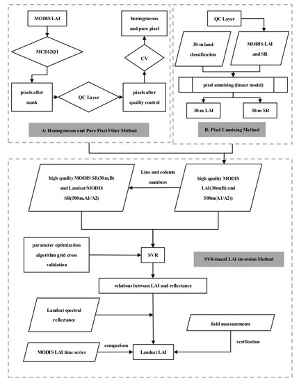
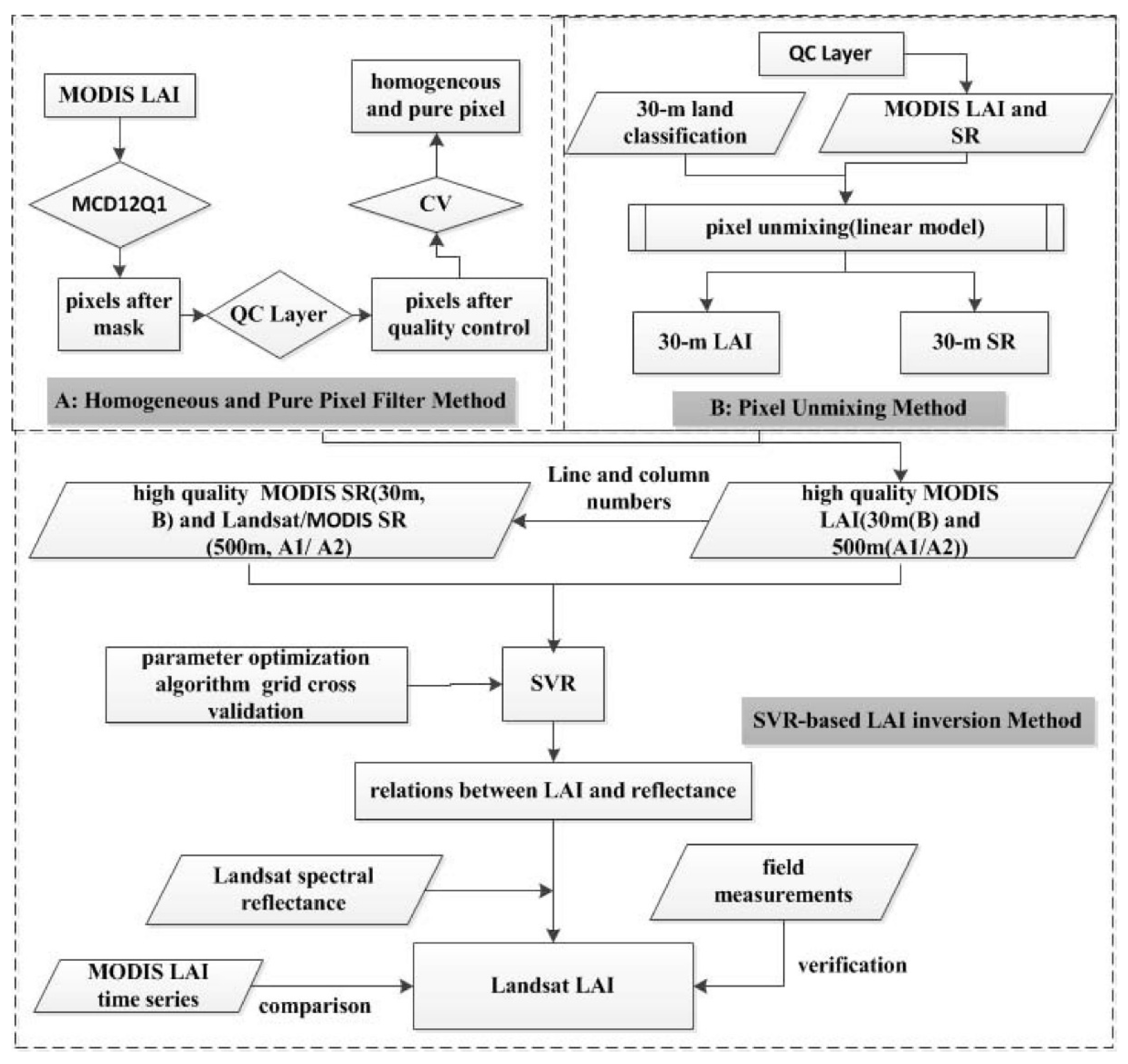
Figure 1 shows the data processing framework. The high-quality training samples of SVR were selected by two methods: the homogeneous and pure pixel filter method (method A) and the pixel unmixing method (method B). For the homogeneous and pure pixel filter method, after the homogeneous and pure MODIS LAI pixels were selected, the upscaled Landsat reflectance (aggregate from 30-m to the 500-m resolution in the ENVI software, using a simple average method) of the corresponding pixels (the same location with the above homogeneous and pure MODIS LAI pixels) together with the LAI were selected as the training samples (dataset A1). Next, the corresponding MODIS reflectance of the pixels together with the LAI were also selected as the training samples (dataset A2). The pixel unmixing method took the unmixed LAI after quality control and reflectance of agricultural land pixels at the 30-m resolution as training samples (dataset B), which were obtained through the unmixing of MODIS LAI and reflectance products by linear models. The SVR models trained by the above three sets of training samples for the two methods were then applied to the Landsat surface reflectance to generate the 30-m resolution LAI. The retrieved LAI maps at the 30-m resolution and the temporal trends curves were generated and analyzed. The retrieval LAI results were then compared to the field measurements.

2.1. Methods of Training Sample Selection

2.1.1. The Homogeneous and Pure Pixel Filter Method

The homogeneous and pure pixel filter method chose the high-quality MODIS LAI pixels by three steps: (1) masking the LAI product images of the research area using MODIS land-cover products (MCD12Q1) to obtain the agricultural land area. According to the International Geosphere-–Biosphere Programme (IGBP) global vegetation type classification dataset (Land Cover Type 1), the pixels with the successive agricultural land type in every year during the research period are considered as the agricultural land area; (2) selecting the high-quality LAI pixels using quality control files (MODIS LAI QC layer) to ensure that the pixels’ LAI are retrieved from the main algorithm, namely, the look-up table (LUT) algorithm. Through the first two steps, we obtain high-quality LAI pixels of agricultural land, and these pixels are used as the input pixels of the third step: (3) filtering the remaining LAI pixels by the coefficients of variation (CV) to select homogeneous and pure pixels.

It is known that the relationship between the LAI and the spectral reflectance or vegetation index is nonlinear. The relationships vary for pure and mixed pixels at low spatial resolution. To model the relationship between the LAI and the spectral reflectance for different vegetation types, pure pixels should be selected as training samples. The spectral reflectance of different objects in a mixed pixel is different. We use the CV (ratio of standard deviation to the mean value) in a statistical model to represent this difference, similarly to in [21].

The CV formula is as follows:

$$\mathrm{CV}=\frac{\mathsf{\sigma }}{\mu }$$

(1)

where CV is the coefficient of variation and σ and μ are the standard deviation and mean of the surface reflectance of the Landsat pixels within a MODIS pixel, respectively.

The CV of the reflectance of each band was calculated for all Landsat pixels at the MODIS pixel scale, and a threshold was determined based on the pixels’ quality and quantity. It is assumed that the MODIS pixels are pure pixels when the CV is small.

When the homogeneous and pure pixels of the MODIS LAI products were selected, the corresponding MODIS surface reflectances were also chosen together to act as the training samples (dataset A2). The MODIS reflectance products have a good correspondence with the MODIS LAI products because of having the same temporal and spatial resolution, with no geometric deviation. In addition, the upscaled Landsat reflectances at the 500-m resolution were aggregated to create another training sample (dataset A1), which allows comparison of these retrieved high-resolution LAI of the training samples for the different selection methods.

2.1.2. The Pixel Unmixing Method

At 500-m resolution, different land cover types may be mixed within a MODIS pixel. The surface reflectance is determined by the spectral characteristics of the different types. Pixel unmixing methods can decompose the pixels of coarse-resolution satellite imagery into different endmembers using high-resolution satellite imagery classification data. These methods can thus obtain the ratio of each type to the coarse-resolution pixel (as a proportion). Ichoku et al. summarized five mixture models. These models are the linear model, the probabilistic model, the geometric-optical model, the stochastic geometric model, and the fuzzy model [28]. In this study, the linear model was used to unmix the MODIS surface reflectance and MODIS LAI. The linear model is a special case of a nonlinear model that ignores multiple scattering [29]. In the linear model, it is assumed that the reflectance of a pixel is a linear combination of the reflectance of each endmember [30]. The weight of the reflectance of the feature type is determined by the ratio of each type to the area of the pixel:

$$\mathrm{R}={\displaystyle \sum }_{j=1}^n\left({\mathrm{f}}_{\mathrm{j}}\times {\mathrm{r}}_{\mathrm{j}}\right)+\epsilon$$

(2)

where $R$ is the reflectance of the mixed pixel; $r_j$ is the reflectance of the j^th endmember; $f_j$ is the proportion of the j^th endmember in the mixed pixel, which can be calculated based on the 30-m land cover map from the Landsat image; and ε is the error. In Equation (2), R and $f_j$ are known, and the unknown variable is the $r_j$. In the study, we assume that the neighboring pixels with the same land cover type have similar surface reflectance or LAI [31]. When the number of endmembers is determined, the number of equations must be greater than or equal to the number of endmembers ($\mathrm{j}$) in order to solve the equation. By using other pixels adjacent to the pixel being processed, one can avoid the ill-conditioning problem caused by too many unknown values, and this can be achieved by sliding the 3 × 3 window [32]. For each mixed pixel, a maximum of nine equations can be derived from the 3 × 3 window, which traverses the entire study area. Each equation group was solved by the constrained least squares method.

The unmixed pixels of MODIS LAI and surface reflectance products at the 30-m resolution using the above method was obtained. Then, choose the pixels of agricultural land cover type and the LAI retrieved from the main algorithm using quality control. Finally, the unmixed MODIS surface reflectance and LAI of the above chosen corresponding pixels were taken as the training samples for SVR.

2.2. Support Vector Regression

Support vector regression (SVR) is a supervised machine-learning method based on the principles of the Vapnik–Chervonenkis dimension theory and structural risk minimization [33]. SVR is more suitable for small samples and nonlinear, high-dimensional problems. SVR aims to construct an optimal super-pipe so that the pipeline can provide as much data as possible under a given accuracy ε, and so that the distance from the sample point to the pipe edge is not larger than ε [34]. This can be expressed by Equation (3):

$$\mathrm{f}\left(\mathrm{x}\right)=\left(\omega ,\phi \left(x,x_i\right)\right)+\mathrm{b}$$

(3)

where $\omega$ is the normal vector (or the “support vector”), $x_i$ stands for the dataset, and $\mathrm{b}$ is the bias.

The loss function in ε-SVR can be expressed as Equation (4):

$${\mathrm{L}}_{\mathsf{\epsilon }}=\{\begin{array}{c}0 \left|\mathrm{y}-\mathrm{f}\left(\mathrm{x}\right)\right|\le \epsilon \\ \left|\mathrm{y}-\mathrm{f}\left(\mathrm{x}\right)\right|-\epsilon \mathrm{otherwise}\end{array}$$

(4)

Operating on the basis of the structural risk minimization theory, SVR finally evolves into a convex optimization problem. Here, the slack variables ${\mathsf{\xi }}^{*}{}_{\mathrm{i}}$ and ${\mathsf{\xi }}_{\mathrm{i}}$ are introduced to represent the fitting error:

$$\mathrm{Min}\frac{1}{2}\Vert \mathsf{\omega }{\Vert }^2+\mathrm{C}{\sum }_{\mathrm{i}=1}^{\mathrm{n}}\left({\mathsf{\xi }}_{\mathrm{i}}+{{\mathsf{\xi }}^{*}}_{\mathrm{i}}\right)$$

(5)

$$\mathrm{subject}\mathrm{to}\{\begin{array}{c}{\mathrm{y}}_{\mathrm{i}}-f\left({\mathrm{x}}_{\mathrm{i}}\right)\le \epsilon +{\mathsf{\xi }}_{\mathrm{i}}^{*}\\ f\left({\mathrm{x}}_{\mathrm{i}}\right)-{\mathrm{y}}_{\mathrm{i}}\le \epsilon +{\mathsf{\xi }}_{\mathrm{i}}\\ {\mathsf{\xi }}_{\mathrm{i}}、{{\mathsf{\xi }}^{*}}_{\mathrm{i}}\ge 0，i=1\dots \dots n\end{array}$$

where $\mathrm{C}$ is the margin parameter.

SVR has the advantage of solving the nonlinear problem by introducing a kernel function, which is a good solution to the problem in high-dimensional space and is the core of SVR. The radial basis function (RBF) has been found to be superior to other kernel functions for reflecting the nonlinear relationship between LAI and reflectance. Therefore, the RBF was used in this research. After that, the choice of hyperparameters determines the quality of the model, which affects the quality of the SVR algorithm. The range of hyperparameters and kernel parameters was [–10, 10], and the six-fold cross-validation method was used to find the optimal parameters. As is well known, the higher the proportion of training samples, the closer the inversion results will be to the measured values. Next, the proportion of training samples was fixed at 80% for optimal parameter determination.

Three inversion models were built through training the SVR algorithm using the three training samples datasets obtained by the homogeneous and pure pixel filter method (datasets A1 and A2, method A) and the pixel unmixing method (dataset B, method B), both of which were described in detail in Section 2.1. In the inversion process, Landsat surface reflectance was used as the input to the three SVR inversion models to retrieve high-resolution LAI at 30-m resolution.

3. Study Area and Data Description

3.1. Study Area

Two study sites were selected in this study. The first study area was located at the boundary between Baoding and Shijiazhuang in the Hebei Province, China (Figure 2a). This area is flat, with about a 40-m altitude. Crops can be harvested twice a year and consist mainly of winter wheat and summer maize. The winter wheat-growing season is from October to June of the following year. The second study area was located near the capital of Iowa in Des Moines, Iowa, United States (Figure 2b), at a 300-m altitude, where the highest temperature occurs in July and the main crops are corn and soybean. The two research areas include three different crops and have different crop cultivation (crops can be harvested once or twice a year). Moreover, the results of the two different study sites could be used to test the robustness of the algorithm and different sampling strategies.

3.2. Data and Preprocessing

The satellite image datasets consisted mainly of MODIS products and Landsat scenes. MODIS products include a land-cover type product (MCD12Q1) (Collection 5 version), LAI products (MCD15A2H), and reflectance products (MOD09A1) (Collection 6 version). Landsat8 operational land imager (OLI) and Landsat5 thematic mapper (TM) and enhanced thematic mapper plus (ETM+) surface reflectance products at the 30-m spatial resolution were also collected as input data. At the Baoding study area, 29 Landsat8 scenes (paths 123–124 and row 33) from April 2013 to May 2017 were selected. In Des Moines, 29 Landsat5 scenes (paths 26–27 and row 31) from May 2003 to August 2007 were chosen. All data were downloaded from https://earthexplorer.usgs.gov/. The blue band in Landsat imagery is susceptible to atmospheric scattering, and the shortwave infrared (SWIR) band differs greatly in the Landsat and MODIS bands (

Table 1. The comparison of band wavelengths between Landsat and MODIS.

Band	TM (μm)	ETM+ (μm)	OLI (μm)	MODIS (μm)
Blue	0.45–0.53	0.45–0.53	0.45–0.51	0.459–0.479
Green	0.52–0.60	0.52–0.60	0.53–0.59	0.545–0.565
Red	0.63–0.69	0.63–0.69	0.64–0.67	0.62–0.67
NIR	0.76–0.90	0.76–0.90	0.85–0.88	0.841–0.876
SWIR	1.55–1.75	1.55–1.75	1.57–1.65	1.628–1.652

). To obtain more band information, this study used the green, red, and near-infrared (NIR) bands.

For classification products, the IGBP global vegetation type classification dataset (Land Cover Type 1) of the MODIS land-cover product (MCD12Q1) is obtained from Terra and Aqua observations over one year, and has 17 main land-cover types [35]. The spatial overlay analysis of the multiyear data to yield the continuous planted area of crops was done to separate the study region into crop and noncrop areas. The spatial overlay analysis method means image binarization, in which a crop pixel is replaced by 1 and a noncrop pixel is replaced by 0, based on MCD12Q1. Then, the binary value of each pixel for every year is multiplied, so 1 stands for the continuous planted area of crops and 0 stands for noncrop areas. The GlobeLand30 product is the global 30-m resolution land-surface cover product generated by the National Geomatics Center of China with the support of ‘863’ key projects, and has 10 main land-cover types. However, it only produced global land cover maps in 2000 and 2010. (The data set is provided by the National Geomatics Center of China. (DOI: 10.11769/GlobeLand30.2000.db; DOI: 10.11769/GlobeLand30.2010.db) [36,37]).

The MODIS LAI was produced by two algorithms: the LUT main algorithm and the backup algorithm, which is an empirical model relating the LAI and the vegetation index [38]. The quality of MODIS LAI for each pixel is described by the quality control flags of the QC layer, which is generally reflected by the SCF_QC bit. The latter three bits of that describe the LAI inversion algorithm [39]. When the SCF_QC is “000”, the main algorithm is used with no saturation, which represents the best-quality LAI.

Field measurements from Des Moines, Iowa, United States were obtained from the 2002 soil moisture experiment (SMEX02) conducted by the U.S. Department of Agriculture (USDA). The purpose of the experiment was to research land–gas interaction, verify ground parameters’ accuracy, and evaluate the new method of monitoring soil moisture by remote sensing. Samples of LAI were obtained using LAI-2000 instruments in the inter-row region at least 1 m away from where the biomass sample was taken [40]. The LAI measurements campaign went through four sampling rounds, conducted over the periods: 15–19 June, 27–30 June, 2–3 July, and 5–9 July. Twelve large areas went through the four rounds. Each observation area covered approximately one MODIS pixel, and each region was spaced to small areas measured three or four times (Figure 2). To match the time of the satellite imagery acquisition, the measured LAI were linearly interpolated to the Landsat data-acquisition time. In situ LAI measurements that had been taken four times were interpolated to the Landsat data-acquisition time. In this study, the LAI measurements on 30 June and 2 July constrained or corresponded to the 1 July inversion results, and the LAI measurements on 7 and 9 July constrained or corresponded to the 8 July inversion results.

Field measurements in Baoding, Hebei Province, China were collected from 27 April to 3 May 2016 using LAI-2000, containing ten sampling points. Measurements from each site were collected at least twice. The corresponding Landsat data-acquisition times were 25 April and 4 May, and the inversion LAI were linearly interpolated to each sampling-point time.

4. Experiments and Analysis

4.1. SVR Training Samples

4.1.1. Homogeneous and Pure Pixel Filter

In this part of the experiment, different experimental areas and different input data (upscaled Landsat reflectance or MODIS reflectance) made the size of the study area different. For example, a 143 × 140 (68,640 m × 67,200 m) pixel region in Des Moines, Iowa, United States was initially selected, and 971 noncrop land pixels were removed after masking using the MODIS land-cover product. Using the SCF_QC layer, the MODIS LAI pixels with the highest quality (SCF_QC = 000, main algorithm and no saturation) were extracted. This process removed 1858 pixels.

The reflectances of the Landsat bands were used in the CV calculation (Equation (1)). The CVs of the Landsat bands were calculated at the MODIS pixel scale using Landsat pixels, followed by the QC checking area, and a threshold of CV for pure pixels was determined based on the pixel quality and quantity. In this paper, a threshold of CV of 0.15 for pure pixels was determined for SMEX02 in the Des Moines area. In order to compare the inversion results of these two sites in the paper and conduct validation of the threshold, the threshold for the Baoding area was the same as that in the Des Moines area. The pure pixel filtering step removed 6090 pixels for one tile after using CV filtering from the NIR of Landsat5. Figure 3 shows the results of each step using the MODIS LAI product on the day 201 of 2005 as an example.

4.1.2. Pixel Unmixing

Taking the SMEX02 site area as an example, the area was mainly composed of natural vegetation and crops. Corn and soybean accounted for >80% of the total area. Figure 4 shows the MODIS classification map (Figure 4a) and the 30-m resolution GlobeLand30 surface covering products (Figure 4b,c). The study area included three categories from the MCD12Q1_IGBP classification system: number 12: agricultural land; number 13: urban and construction area; and number 14: junction of agricultural land and natural vegetation. The following classification of the GlobeLand30 product is used: arable land (10), forest (20), grassland (30) (accounting for 5% of the total area), wetland (50) (accounting for ~1% of the total area), water body (60), artificial surfaces (80), and bare land (90).

In this paper, the study area was divided into arable land, artificial surface, forest, grassland, and water bodies. Based on the Landsat scenes from 14 May to 2 August in 2002, it was obvious that the arable land had a regular shape and the spectral characteristics were different from other types. In addition, roads (within the artificial surface category) showed a regular rectangle, especially the roads between arable lands. This study used an object-oriented segmentation approach to classify the Landsat imagery. The eCognition software was used for this. Finally, the classification results were corrected by visual interpretation. Figure 4d shows the final results.

In this paper, a linear model was used to solve the mixed pixels, using the algorithm presented in Equation (3). A 3 × 3 sliding window was used to obtain the optimal solutions to the sets of equations. The MODIS surface reflectance and LAI products were unmixed by this method, described in Section 2. For example, in the SMEX02 study area, 5300 MODIS pixels were used to obtain the unmixing pixels and 2902 MODIS pixels were removed after QC checking. Finally, fewer than 400 arable land pixels were chosen in one tile (the day 137 of 2003).

4.2. Comparison of Regions

4.2.1. Retrieved LAI on SMEX02

In this part of the experiment, a comparison of the 30-m resolution LAI retrieved from Landsat surface reflectance scenes for three periods by different SVR inversion models and the field measurements was made. Figure 5 shows the results.

Figure 5 shows that the retrieved LAI agrees well with the field measurements. At the field scale, the R² (coefficient of determination) between retrieved Landsat LAI and field measurements is 0.79 for the homogeneous and pure pixel filter method with upscaled Landsat reflectance as the training samples (dataset A1) (Figure 5a). The R² value is 0.81 for the homogeneous and pure pixel filter method with MODIS reflectance as the training samples (dataset A2) (Figure 5b), slightly better than dataset A1. The correlation coefficients of dataset A2 and dataset B was similar (Figure 5b,c), where the retrievals of unmixed MODIS reflectance and LAI using the pixel unmixing method (method B) shown in Figure 5c was slightly higher, with the R² value of 0.82 and a root mean square error (RMSE) value of 0.65. Although we had obtained high-quality pixels through two methods, it was inevitable that the MODIS LAI was small and underestimated due to mixing pixels at the small LAI stage. When the Landsat reflectance at 30-m resolution (the cover area of vegetation categories of the pixel usually is larger than that of MODIS at the small LAI stage) was used as the input for the SVR models, the results were overestimated when LAI was 0–2. We found that the results of approach B were improved when LAI was <2. However, when the LAI was greater than 3, the inversion results were significantly underestimated, especially on 8 July (Figure 6) [21]. One reason for this could be that, generally, the relationship between LAI and reflectance gradually becomes saturated. Another reason for the underestimation may have been that when the LAI was >3, especially when the LAI was much greater, the MODIS inversion algorithm was mainly using the backup algorithm on SMEX02, and the training samples obtained using the LUT method contained fewer pixels of LAI > 3. The result was that the training sample representativeness with LAI greater than 3 was poor. It is also clear that the mixed-pixel decomposition method had higher accuracy on 1 and 8 July due to the removal of other vegetation types (mainly forest and grassland, which grew better from June–July), and LAI also showed an increasing trend.

4.2.2. Retrieved LAI at the Baoding Study Area

In the present study, the red, near-infrared, and green bands of the Landsat scene were extracted to retrieve 30-m resolution LAI. Figure 7 shows the results of a comparison with measured values. The results of approach A1 and A2 compared with the measured values is shown in Figure 7a: the R² is 0.77 and the RMSE is 0.41 of A in general, and the inversion and measured values showed good correlation. The retrievals of approach B shown in Figure 7b were slightly higher, with the R² value of 0.79 and an RMSE value of 0.49. However, as the LAI value becomes larger, the inversion value is gradually more severely underestimated, and large deviations from the measured values occurred for the same reason as with SMEX02.

4.2.3. Temporal Trends of LAI at the 30-m Resolution

In this research, Landsat LAI maps at the 30-m resolution at the SMEX02 site were retrieved for three periods, namely, 23 June, 1 July, and 8 July. The three SVR inversion models of datasets A1, A2, and B were used and compared. In Figure 8, no matter which inversion method was used, the LAI inversion values increased over time. Furthermore, they all had a good agreement with the distribution of vegetation in space. The Landsat LAI maps showed that different inversion methods had similar inversion results, and that it was also consistent with the comparison between retrievals and field measurements in Section 4.2.1.

In the Baoding area, ten measurements were located in seven valid MODIS pixels. The Landsat acquisition time extended from 2 April to 4 May, with a total of five measurement dates (2 April, 9 April, 18 April, 25 April, and 4 May). The temporal trend of LAI at the 30-m resolution was compared with that of the MODIS LAI (Figure 9).

The results show that the LAI time series retrieved from the Landsat data was consistent with the trend of the MODIS LAI time series (taking six pixels as an example). On the whole, the LAI curve showed a tendency to rise first and then decline, and reached the maximum near day of year (DOY) = 113. For Figure 9c, the CV of the pixel was >0.15, so this pixel is not pure and homogenous. In most situations, the LAI values of Landsat were higher than the MODIS LAI values, possibly mainly due to mixed pixels, among others. In the MODIS scale, the pixel contains nonvegetation categories and affects the MODIS LAI, but in the Landsat scale, the cover area of vegetation categories of the pixel usually is larger than that of MODIS. Of course, there are other errors, such as the scale effect, and so forth.

5. Discussion

A comparative analysis of accuracy between the LAI retrievals and the field measurements (or MODIS LAI) was performed for the homogeneous and pure pixel filter method (method A) and the pixel unmixing method (method B). The results demonstrated that inversion of high-resolution LAI combining MODIS products based on the SVR algorithm was feasible. Compared to physical modeling methods, the empirical model using the SVR algorithm did not need to consider the physiological characteristics of vegetation and was easy to implement. Compared to other methods of obtaining training samples, our methods can obtain a greater number of high-quality samples based on global LAI products.

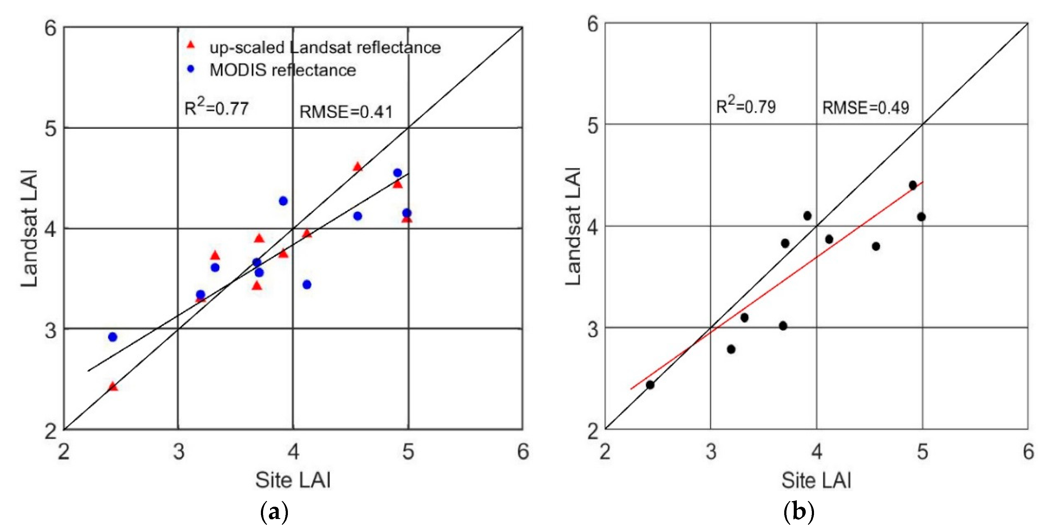
Gao et al. [21] used the decision tree with the upscaled Landsat reflectance at the 500-m resolution and MODIS LAI to retrieve LAI at the 30-m resolution. The comparison (R² = 0.79, mean bias error = −0.18, mean absolute difference = 0.58) between Landsat retrievals (30-m) of Gao’s and field measurements at the field scale (10-m) showed that there was a good agreement with low to moderate LAI (0–3), but retrievals were underestimated for high LAI (3–5). In this paper, the R² was 0.79 and the RMSE was 0.73 for the homogeneous and pure pixel filter method when the MODIS LAI and upscaled Landsat reflectance at the 500-m resolution were used as the training samples (dataset A1). The R² was 0.81 and RMSE was 0.69 for the homogeneous and pure pixel filter method when the MODIS LAI and reflectance were used as the training samples (dataset A2). In addition, the retrievals of the unmixing method with unmixed MODIS reflectance and LAI at the 30-m resolution as the training samples (dataset B) were slightly higher, with an R² value of 0.82 and an RMSE value of 0.65. Compared with Gao et al., we selected the multiyear MODIS products for obtaining training samples to ensure the richness and representativeness of the samples. In addition, the MODIS LAI and reflectance products were also used as training samples to build the SVR inversion model, and yielded a good result. Moreover, the pixel unmixing method was used to obtain the SVR inversion model, and resulted in the highest accuracy.

In particular, the SVR algorithm had an advantage in solving the nonlinear problem because it overcomes the phenomena of “over-learning” and “under-learning” [41]. After the kernel function and the hyperparameters were chosen, the relationship between the MODIS LAI and surface reflectance was fitted. It was shown that the SVR algorithm can represent the relationship between LAI and reflectance and had good generalization ability.

Moreover, the quality of the training samples, including sample distribution, can seriously affect the quality of all empirical approaches, including the SVR. In this study, the training samples spanned multiple years and included the whole crop-growing season. Therefore, the data quality was good and representative. The homogeneous and pure pixel filter method took the quality control file (QC layer) of the MODIS LAI products into consideration and ensured the quality of the MODIS LAI. This was the precondition for taking the MODIS LAI as training samples. The ratio of the standard deviation to the mean value (CV) in a statistical model can represent the difference of spectral reflectance of different objects in a mixed pixel. The MODIS pixels can be considered homogeneous and pure pixels when the thresholds of the QC and CV settle within a certain range. The pixel unmixing method decomposed the pixels of coarse-resolution satellite imagery into different endmembers and obtained the high-resolution LAI (or reflectance). It can obtain higher-quality training samples than other methods.

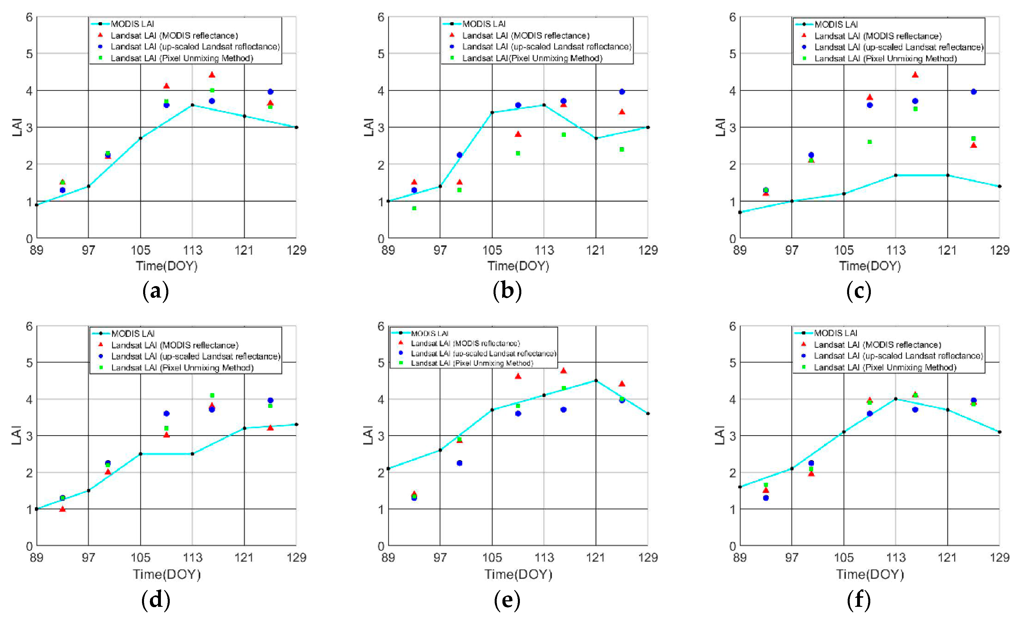
However, there were also a few limitations to be improved upon. First, when the LAI was greater than 3, the inversion results were underestimated during July. A main reason for this was that the relationship between the surface reflectance and LAI tended to become saturated when the LAI was greater than 3. In this paper, when the MODIS LAI is high, the probability of using the main algorithm is low. In other words, if the training samples were selected by the main algorithm, many samples with LAI > 3 were eliminated, resulting in fewer training samples with high LAI values. Figure 10 shows the histogram of LAI from the LAI-SR samples of SMEX02. As we can see from the histogram, there are fewer large LAI values (>3.0). In the SMEX02, there are 21,500 LAI-SR samples for dataset A1; 2028 for dataset A2, using the homogeneous and pure pixel filter method; and 17,889 for the pixel unmixing method. In Baoding, the LAI-SR samples are 6909, 8797, and 8838, respectively. In addition, the scaling effect may cause the under-representation of high LAI values. The high values can be smoothed out in the coarse-resolution image. For both training sample-acquiring methods, we used the MODIS quality control flags to select the highest-quality retrievals derived from the MODIS LAI main algorithm. We relied on the MODIS LAI data quality flags and have not considered the effect of noise associated with the main algorithm. The noise from the main algorithm retrieval may need to be considered for other regions, such as the tropical area, where clouds are always present.

Furthermore, when the upscaled Landsat reflectance and MODIS LAI were used to build the relational model, geometrical registration between Landsat and MODIS was not performed in this study. This led to a bias when calculating the CV of the Landsat surface reflectance in a MODIS pixel. The CV threshold of the homogeneous MODIS pixel was determined based on LAI sample quality and quantity from subjective experience at present. The threshold may vary with different study sites or landscapes. In order to compare the inversion results from these two sites in the paper, the same threshold of 0.15 was used. Additional study and analysis are needed to quantify the threshold. In this paper, we used the eight-day MODIS LAI products. This means that the MODIS LAI product for the period was made up from eight independent days. However, the Landsat imagery reflected the instantaneous optical characteristics of vegetation for the Landsat acquisition date. Therefore, differences between the Landsat and MODIS data products were observed in time and space.

Note that the spectral response function of the sensor is different, and the wavelengths of the corresponding bands are also different. The spectral response function of the sensor is a function of the wavelength. It is the ratio of the radiance received by the sensor at each wavelength to the radiance of the incident. In this study, we compared the bands of Landsat and MODIS and chose the three bands with small difference. Although the relational model was built using MODIS reflectance and MODIS LAI, the Landsat reflectance was used as the input parameter to retrieve the LAI. There exists a large gap in the wavelength range, particularly in the near-infrared band4 of Landsat5. Thus, the use of a spectral response function to convert the Landsat reflectance and MODIS reflectance will be the next key work.

Finally, an empirical model has advantages, but also limitations. In this study, the verification experiments were conducted over two study areas: the Hebei Province, China and Des Moines, Iowa, United States. Crops included corn, soybean, and winter wheat. Although the inversion model proposed here achieved good results in the study area, applications in other areas need to be further verified. To apply the model to large regions, not only must the method of screening high-quality data be improved, but the biophysical mechanisms of vegetation must also be studied. In the present study, the relationship between LAI and reflectance had a certain scope of application. Moreover, inversion accuracy was high in the main growth period, but was reduced in other periods, especially in the late stages of crop growth. Climate change may impact vegetation growth. The accuracy of LAI retrieval may be decreased if LAI-SR samples cannot cover this variation. In our study sites, climate change from the study period is not significant to enable testing of this hypothesis. Future research may consider different inversion models at different times.

6. Conclusions

In this study, a support vector regression algorithm combined with MODIS LAI and reflectance products which were used to obtain training samples was developed to retrieve high-resolution LAI from Landsat data. The homogeneous and pure pixel filter method and the pixel unmixing method were applied to select high-quality training samples to retrieve high-resolution LAI. Among them, the principle of selecting training samples for the homogeneous and pure pixel filter was simple and easy to operate. Additionally, the pixel unmixing method took into account the problem of mixed pixels in the large scale. The results of the two main methods were in good agreement with the field-measured values. Inversion accuracy of the pixel unmixing method was slightly higher than the homogeneous and pure pixel filter method, but the pixel unmixing method was more complex to implement. Using the homogeneous and pure pixel filter method, the retrievals using MODIS reflectance as the training samples was better than upscaled Landsat reflectance as the training samples. These tests showed that both methods combined with MODIS products can retrieve 30-m resolution LAI from Landsat imagery. In future research, additional validations need to be done to assess the accuracy of the approach over other regions.

References

1. Chen, J.M.; Black, T.A. Measuring leaf area index of plant canopies with branch architecture. Agric. For. Meteorol. 1991, 57, 1–12. [Google Scholar] [CrossRef]
2. Barbu, A.L.; Calvet, J.C.; Mahfouf, J.F.; Albergel, C.; Lafont, S. Assimilation of soil wetness index and leaf area index into the ISBA-A-gs land surface model: Grassland case study. Biogeosci. Discuss. 2011, 8, 1971–1986. [Google Scholar] [CrossRef] [Green Version]
3. Anav, A.; Murray-Tortarolo, G.; Friedlingstein, P.; Sitch, S.; Piao, S.; Zhu, Z. Evaluation of land surface models in reproducing satellite derived leaf area index over the high-latitude northern hemisphere. Part II: Earth system models. Remote Sens. 2013, 5, 3637–3661. [Google Scholar] [CrossRef] [Green Version]
4. Zhu, Z.; Bi, J.; Pan, Y.; Ganguly, S.; Anav, A.; Xu, L.; Samanta, A.; Piao, S.; Nemani, R.; Myneni, R. Global data sets of vegetation leaf area index (LAI)3g and fraction of photosynthetically active radiation (FPAR)3g derived from global inventory modeling and mapping studies (GIMMS) normalized difference vegetation index (NDVI3g) for the period 1981 to 2011. Remote Sens. 2013, 5, 927–948. [Google Scholar] [CrossRef]
5. Claverie, M.; Matthews, J.; Vermote, E.; Justice, C. A 30+ year AVHRR LAI and FPAR climate data record: Algorithm description and validation. Remote Sens. 2016, 8, 263. [Google Scholar] [CrossRef]
6. Myneni, R.B.; Hoffman, S.; Knyazikhin, Y.; Privette, J.L.; Glassy, J.; Tian, Y. Global products of vegetation leaf area and fraction absorbed par from year one of MODIS data. Remote Sens. Environ. 2002, 83, 214–231. [Google Scholar] [CrossRef]
7. Xiao, Z.; Liang, S.; Wang, J.; Chen, P.; Yin, X.; Zhang, L.; Song, J. Use of general regression neural networks for generating the GLASS leaf area index product from time-series MODIS surface reflectance. IEEE Trans. Geosci. Remote Sens. 2014, 52, 209–223. [Google Scholar] [CrossRef]
8. Baret, F.; Hagolle, O.; Geiger, B.; Bicheron, P.; Miras, B.; Huc, M.; Berthelot, B.; Niño, F.; Weiss, M.; Samain, O.; et al. LAI, FPAR and fCover CYCLOPES global products derived from VEGETATION. Part 1: Principles of the algorithm. Remote Sens. Environ. 2007, 110, 275–286. [Google Scholar] [CrossRef] [Green Version]
9. Baret, F.; Weiss, M.; Lacaze, R.; Camacho, F.; Makhmara, H.; Pacholcyzk, P.; Smets, B. Geov1: LAI and FPAR essential climate variables and fCover global time series capitalizing over existing products. Part 1: Principles of development and production. Remote Sens. Environ. 2013, 137, 299–309. [Google Scholar] [CrossRef]
10. Hu, J.; Tan, B.; Shabanov, N.; Crean, K.A.; Martonchik, J.V.; Diner, D.J.; Knyazikhin, Y.; Myneni, R.B. Performance of the MISR LAI and FPAR algorithm: A case study in africa. Remote Sens. Environ. 2003, 88, 324–340. [Google Scholar] [CrossRef]
11. Valderrama-Landeros, L.H.; España-Boquera, M.L.; Baret, F. Deforestation in Michoacan, Mexico, from CYCLOPES-LAI time series (2000–2006). IEEE J. Sel. Top. Appl. Earth Obs. Remote Sens. 2017, 1–8, 1–8. [Google Scholar] [CrossRef]
12. Wang, J.; Wang, J.; Zhou, H.; Xiao, Z. Detecting forest disturbance in northeast China from GLASS LAI time series data using a dynamic model. Remote Sens. 2017, 9, 1293. [Google Scholar] [CrossRef]
13. Wang, Q.; Tenhunen, J.; Dinh, N.; Reichstein, M.; Otieno, D.; Granier, A.; Pilegarrd, K. Evaluation of seasonal variation of MODIS derived leaf area index at two European deciduous broadleaf forest sites. Remote Sens. Environ. 2005, 96, 475–484. [Google Scholar] [CrossRef]
14. Verrelst, J.; Rivera, J.P.; Veroustraete, F.; Muñoz-Marí, J.; Clevers, J.G.P.W.; Camps-Valls, G.; Moreno, J. Experimental sentinel-2 LAI estimation using parametric, non-parametric and physical retrieval methods—A comparison. ISPRS J. Photogramm. Remote Sens. 2015, 108, 260–272. [Google Scholar] [CrossRef]
15. Zhang, W.; Chen, Y.; Hu, S. Retrieving LAI in the heihe and the hanjiang river basins using Landsat images for accuracy evaluation on MODIS LAI product. Int. Geosci. Remote Sens. Symp. (IGARSS) 2007, 3417–3421, 3417–3421. [Google Scholar] [CrossRef]
16. Chen, J.M.; Pavlic, G.; Brown, L.; Cihlar, J.; Leblanc, S.G. Derivation and validation of Canada-wide coarse-resolution leaf area index maps using high-resolution satellite imagery and ground measurements. Remote Sens. Environ. 2002, 80, 165–184. [Google Scholar] [CrossRef]
17. Duan, S.B.; Li, Z.L.; Wu, H.; Tang, B.H.; Ma, L.; Zhao, E.; Li, C. Inversion of the PROSAIL model to estimate leaf area index of maize, potato, and sunflower fields from unmanned aerial vehicle hyperspectral data. Int. J. Appl. Earth Obs. Geoinf. 2014, 26, 12–20. [Google Scholar] [CrossRef]
18. Durbha, S.S.; King, R.L.; Younan, N.H. Support vector machines regression for retrieval of leaf area index from multiangle imaging spectroradiometer. Remote Sens. Environ. 2007, 107, 348–361. [Google Scholar] [CrossRef]
19. Huang, J.; Li, X.; Liu, D.; Ma, H.; Tian, L.; Wei, S. Comparison of winter wheat yield estimation by sequential assimilation of different spatio-temporal resolution remotely sensed LAI datasets. Trans. Chin. Soc. Agric. Mach. 2015, 46, 240–248. [Google Scholar] [CrossRef]
20. Chen, S.; Zhao, Y.; Shen, S. Applicability of pywofost model based on ensemble kalman filter in simulating maize yield in northeast China. Chin. J. Agrometeorol. 2012, 33, 245–253. [Google Scholar]
21. Gao, F.; Anderson, M.C.; Kustas, W.P.; Wang, Y. Simple method for retrieving leaf area index from Landsat using MODIS leaf area index products as reference. J. Appl. Remote Sens. 2012, 6, 063554. [Google Scholar] [CrossRef]
22. Viña, A.; Gitelson, A.A.; Nguy-Robertson, A.L.; Peng, Y. Comparison of different vegetation indices for the remote assessment of green leaf area index of crops. Remote Sens. Environ. 2011, 115, 3468–3478. [Google Scholar] [CrossRef]
23. Wang Qing, L.J.; Kun-Yong, Y. Inversion of masson pine forest LAI by multiple-perspective vegetation index. Plant Sci. J. 2017, 35, 48–55. [Google Scholar] [CrossRef]
24. Linna, C.; Yonghua, Q.; Lixin, Z.; Shunlin, L.; Jindi, W. Estimating time series leaf area index based on recurrent neural networks. Adv. Earth Sci. 2009, 24, 756–768. [Google Scholar] [CrossRef]
25. Liang, S.L.; Cheng, J.; Jia, K.; Jiang, B.; Liu, Q.; Liu, S.H.; Xiao, Z.Q.; Xie, X.H.; Yao, Y.J.; Yuan, W.P.; et al. Recent progress in land surface quantitative remote sensing. J. Remote Sens. 2016, 20, 875–898. [Google Scholar] [CrossRef]
26. Lv, J. Hyperspectral Remote Sensing Inversion Models of Crop Chlorophy || Content Based on Machine Learning and Radiative Transfer Models; China University of Geosciences: Beijing, China, 2012. [Google Scholar]
27. Awad, M.; Mariette, R.; Khanna, R. Support vector regression. Neural Inf. Process. Lett. Rev. 2007, 11, 203–224. [Google Scholar]
28. Ichoku, C.; Karnieli, A. A review of mixture modeling techniques for sub-pixel land cover estimation. Remote Sens. Rev. 1996, 13, 161–186. [Google Scholar] [CrossRef]
29. Chang chun, L.V. A review of pixel unmixing models. Remote Sens. Inf. 2003, 55–58, 55–58. [Google Scholar] [CrossRef]
30. Settle, J.J.; Drake, N.A. Linear mixing and the estimation of ground cover proportions. Int. J. Remote Sens. 1993, 14, 1159–1177. [Google Scholar] [CrossRef] [Green Version]
31. Tobler, W.R. A computer movie simulating urban growth in the detroit region. Econ. Geogr. 1970, 46, 234–240. [Google Scholar] [CrossRef]
32. Liao, L.; Song, J.; Wang, J.; Xiao, Z.; Wang, J. Bayesian method for building frequent Landsat-like NDVI datasets by integrating MODIS and Landsat NDVI. Remote Sens. 2016, 8, 452. [Google Scholar] [CrossRef]
33. Vapnik, V.; Golowich, S.E.; Smola, A. Support vector method for function approximation, regression estimation, and signal processing. Adv. Neural Inf. Process. Syst. 1997, 9, 281–287. [Google Scholar]
34. Chang, C.C.; Lin, C.J. Libsvm: A library for support vector machines. ACM Trans. Intell. Syst. Technol. (TIST) 2011, 2, 27. [Google Scholar] [CrossRef]
35. Friedl, M.A.; Sulla-Menashe, D.; Tan, B.; Schneider, A.; Ramankutty, N.; Sibley, A.; Huang, X. MODIS collection 5 global land cover: Algorithm refinements and characterization of new datasets. Remote Sens. Environ. 2010, 114, 168–182. [Google Scholar] [CrossRef]
36. Chen, J.; Ban, Y.; Li, S. China: Open access to earth land-cover map. Nature 2014, 514, 434. [Google Scholar]
37. Chen, J.; Liao, A.; Chen, J.; Peng, S.; Chen, L.; Zhang, H. 30-Meter Global Land Cover Data Product-Globe Land30; Geomatics World: Beijing, China, 2017. [Google Scholar]
38. Knyazikhin, Y.; Glassy, J.; Privette, J.L.; Tian, Y.; Lotsch, A.; Zhang, Y.; Wang, Y.; Morisette, J.T.; Votava, P.; Myneni, R.B.; et al. MODIS Leaf Area Index (LAI) and Fractionof Photosynthetically Active Radiation Absorbed by Vegetation (FPAR) Product (MOD15) Algorithm Theoretical Basis Document. 1999. Available online: http://eospso.gsfc.nasa.gov/atbd/modistables.html (accessed on 11 May 2018).
39. Yang, W.; Huang, D.; Tan, B.; Stroeve, J.C.; Shabanov, N.V.; Knyazikhin, Y.; Nemani, R.R.; Myneni, R.B. Analysis of leaf area index and fraction of par absorbed by vegetation products from the terra modis sensor 2000–2005. IEEE Trans. Geosci. Remote Sens. 2006, 44, 1829–1842. [Google Scholar] [CrossRef]
40. Anderson, M.C.; Neale, C.M.U.; Li, F.; Norman, J.M.; Kustas, W.P.; Jayanthi, H.; Chavez, J. Upscaling ground observations of vegetation water content, canopy height, and leaf area index during SMEX02 using aircraft and Landsat imagery. Remote Sens. Environ. 2004, 92, 447–464. [Google Scholar] [CrossRef]
41. Liang, D.; Yang, Q.; Huang, W.; Peng, D.; Zhao, J.; Huang, L.; Zhang, D.; Song, X. Estimation of leaf area index based on wavelet transform and support vector machine regression in winter wheat. Infrared Laser Eng. 2015, 44, 335–340. [Google Scholar] [CrossRef]
Figure 1. Data processing flowchart of the support vector regression (SVR) inversion method with two training sample-selecting methods: (A) the homogeneous and pure pixel filter method and (B) the pixel unmixing method.
Remotesensing 10 01187 g001
Figure 2. The two study areas: (a) Baoding, Hebei Province, China; (b) Des Moines, Iowa, United States. The grid in (b) shows the MODIS pixel cells at the 500-m resolution.
Remotesensing 10 01187 g002aRemotesensing 10 01187 g002b
Figure 3. The MODIS leaf area index (LAI) pixel filtering process. From left to right: (a) original MODIS LAI; (b) MODIS LAI pixels for cropland with the highest retrieval quality (main algorithm and not saturated); (c) CV map of NIR band4 from Landsat5; and (d) final selected homogeneous and pure MODIS LAI pixels.
Remotesensing 10 01187 g003
Figure 4. Classification products of the Soil Moisture Experiment 2002 (SMEX02) near Des Moines, Iowa, United States: (a) MCD12Q1_IGBP; (b) GlobeLand30 in 2000; (c) GlobeLand30 in 2010; (d) 30-m classification product. Notes: (a) 12: agricultural land; 13: urban and construction area; 14: junction of agricultural land and natural vegetation. (bd) 10: arable land; 20: forest; 30: grassland; 50: wetland; 60: water body; 80: artificial surfaces; 90: bare land.
Remotesensing 10 01187 g004aRemotesensing 10 01187 g004b
Figure 5. The comparison between the retrieved LAI by three approaches and field measurements: (a) the results of dataset A1 (upscaled Landsat reflectance at the 500-m resolution and MODIS LAI products); (b) the results of dataset A2 (MODIS reflectance and LAI products); (c) the results of dataset B (unmixed MODIS surface reflectance and LAI products at 30-m resolution).
Remotesensing 10 01187 g005
Figure 6. Comparison of inversion LAI in time series with field measurements. (ac) The results of dataset A1; (df) the results of dataset A2; (gi) the results of dataset B.
Remotesensing 10 01187 g006
Figure 7. Comparison of inversion LAI with field measurements at the Baoding study area; (a) the results of datasets A1 and A2; (b) the results of dataset B.
Remotesensing 10 01187 g007
Figure 8. The LAI inversion in time series at the SMEX02 site (23 June, 1 July, and 8 July): (a) the results of dataset A1; (b) the results of dataset A2; (c) the results of dataset B.
Remotesensing 10 01187 g008
Figure 9. LAI inversion in time series at the Baoding area (MODIS DOY: 89–129), based on the homogeneous and pure pixel filter method and the pixel unmixing method. (a) pixel one; (b) pixel two; (c) pixel three; (d) pixel four; (e) pixel five and (f) pixel six.
Remotesensing 10 01187 g009
Figure 10. Histogram of LAI from the LAI-SR samples of SMEX02. (a) dataset A1 (upscaled Landsat reflectance at the 500-m resolution and MODIS LAI products); (b) dataset A2 (MODIS reflectance and LAI products); (c) dataset B (unmixed MODIS surface reflectance and LAI products at 30-m resolution).
Remotesensing 10 01187 g010