Hyperspectral Measurement of Seasonal Variation in the Coverage and Impacts of an Invasive Grass in an Experimental Setting


1
School of Forest Resources and Conservation, University of Florida, Gainesville, FL 32611, USA
2
Nelson Institute for Environmental Studies, University of Wisconsin-Madison, Madison, WI 53706, USA
3
Agronomy Department, University of Florida, Gainesville, FL 32611, USA
*
Authors to whom correspondence should be addressed.
Remote Sens. 2018, 10(5), 784; https://doi.org/10.3390/rs10050784
Submission received: 13 April 2018
/
Revised: 4 May 2018
/
Accepted: 14 May 2018
/
Published: 18 May 2018
(This article belongs to the Special Issue Advances in Remote Sensing Applications for the Detection of Biological Invasions)
Abstract
:Hyperspectral remote sensing can be a powerful tool for detecting invasive species and their impact across large spatial scales. However, remote sensing studies of invasives rarely occur across multiple seasons, although the properties of invasives often change seasonally. This may limit the detection of invasives using remote sensing through time. We evaluated the ability of hyperspectral measurements to quantify the coverage of a plant invader and its impact on senesced plant coverage and canopy equivalent water thickness (EWT) across seasons. A portable spectroradiometer was used to collect data in a field experiment where uninvaded plant communities were experimentally invaded by cogongrass, a non-native perennial grass, or maintained as an uninvaded reference. Vegetation canopy characteristics, including senesced plant material, the ratio of live to senesced plants, and canopy EWT varied across the seasons and showed different temporal patterns between the invaded and reference plots. Partial least square regression (PLSR) models based on a single season had a limited predictive ability for data from a different season. Models trained with data from multiple seasons successfully predicted invasive plant coverage and vegetation characteristics across multiple seasons and years. Our results suggest that if seasonal variation is accounted for, the hyperspectral measurement of invaders and their effects on uninvaded vegetation may be scaled up to quantify effects at landscape scales using airborne imaging spectrometers.
1. Introduction
Invasions of non-native plants into terrestrial ecosystems can alter vegetation structure, plant and animal biodiversity, fire regimes, and ecosystem processes, such as nutrient and water cycling [1,2,3,4]. Distribution mapping of invasive plants is important for the early detection of new invasions, the development of management strategies [5], and assessments of the impacts of invasive plants [6]. Remote sensing can be a valuable tool for investigating invasive species because its large spatial coverage and frequent temporal sampling can be used to measure invasive species’ coverage [7,8], phenology [9], and impact on ecosystem structure, diversity, and dynamics [10,11].
Hyperspectral remote sensing can be particularly useful for invasive plant detection [12] because its high spectral resolution can discriminate among plant functional groups and plant species [13]. Additionally, hyperspectral measurements can simultaneously detect multiple plant chemical or structural traits that may be unique to the invasive plant [14] or occur as a result of invader impacts [10]. For example, the invasive iceplant (Carpobrotus edulis) and jubata grass (Cortaderia jubata) in coastal California were identified via hyperspectral images based on their higher leaf water content than native vegetation [15]. Leafy spurge (Euphorbia esula) in the northwestern United States (U.S.) was differentiated by the pigment concentrations of its floral bracts [16], and perennial pepperweed in a California delta was distinguished due to its unique chlorophyll content [17]. Hyperspectral Airborne Visible/Infrared Imaging Spectrometer (AVIRIS) images revealed that invasive Kahili ginger (Hedychium gardnerianum) was found to reduce nitrogen concentration and increase aboveground water content in a Hawaiian montane rain forest [10]. Other studies have used spectral differences to identify senescent vegetation and quantify the canopy water content associated with invasive species [18,19].
Most hyperspectral studies examine the detection of invasive species and their impacts at a single sampling period [20,21], or in the same season across years [17,22]. However, invasive and native plants can have varied vegetative and reproductive phenologies such that hyperspectral discrimination between invasive and native plants differs seasonally. Yang et al. [23] found that the same species can have different leaf traits seasonally, and that detection techniques need to incorporate seasonal change in order to measure traits throughout the year. Furthermore, seasonal changes in the senescence, leaf chemistry, or water content of invasive plants can lead to different impacts on the vegetation community throughout the year. Remote sensing approaches that take into account seasonal and annual variation will be more robust than algorithms developed from data from a single sampling period and are likely to improve the accurate characterization of invasives and their impacts.
In this study, we use hyperspectral data to quantify an invasive species and its impact on vegetation characteristics in different seasons across multiple years. The study focuses on cogongrass (Imperata cylindrica), a non-native invasive in the southeastern U.S. Cogongrass was initially planted in the southeastern United States for forage and soil stabilization [24], but has spread rapidly to roadsides, agricultural fields [25], and native longleaf pine ecosystems [26] of the southeastern U.S. In longleaf pine forests, cogongrass reduces native understory species diversity [27] and alters vegetation properties, such as the amount of dead material and vegetation water content [28]. Fire-promoting species such as cogongrass tend to accumulate dead plant material [29], altering understory composition and fuel cover [1], and potentially stimulating a higher frequency and intensity of burns than historically experienced in longleaf pine forests [30]. The hotter cogongrass-fueled fires can kill low herbs, shrubs, and even normally fire-tolerant longleaf pine saplings [28]. Following fires, cogongrass quickly invades burned areas and creates cogongrass monocultures, which may create a positive feedback loop between cogongrass invasion and intense fire [31]. Several studies have developed algorithms to discriminate cogongrass from other grasses in pastures using hyperspectral data in lab and agricultural settings [32,33]. However, there has been no attempts to quantify the cover of cogongrass in longleaf pine savannas, which have very high understory species diversity [34]. The high spectral heterogeneity that can be expected from high understory species diversity [35,36] could make the quantification of cogongrass from remote sensing more difficult.
We evaluated the predictive ability of remote sensing metrics to measure key vegetation characteristics in an experiment that factorially manipulated cogongrass coverage and rainfall in a longleaf pine grass community [37]. In most cases, the remote sensing of invasive species and their impacts are measured in observational field settings [7,8,17,38] or laboratory settings [32]. Rarely are these measurements made in controlled field experiments where invasive plant presence, the matrix of co-occurring species, and environmental conditions, such as amount of rainfall, are controlled. In this study, we took advantage of an experiment that factorially manipulated invasive plant presence and rainfall in initially similar plant communities to investigate the predictive ability of hyperspectral measurements to quantify the percent cover of an invasive plant species (a federal noxious weed) and key vegetation characteristics, namely dead plant coverage and plant water content. Our objectives were to: (1) quantify how well hyperspectral measurements can detect variation in cogongrass coverage, dead plant material, and water content in an experimentally controlled field setting: and (2) determine how well an algorithm that has been trained in one season can predict ecosystem characteristics in another season.
2. Materials and Methods
The field experiment is located at the Bivens Arm site (29°37′42.4″N, 82°21′14.4″W) near the University of Florida in Gainesville, Florida, U.S. Northern Florida has a humid subtropical climate, with a wet summer season in the summer months and a dry season from early fall through late spring. The wet season typically has high humidity and frequent rainfall, with an average daily high temperature above 28.3 °C and 15.2 cm average precipitation per month. During the dry season from late fall through spring, temperatures are cooler, with monthly average temperatures between 12.4–23.7 °C, and average monthly precipitation between 5.2–10.9 cm. The soils used in the experiment are Portsmouth sandy loam [37].
Forty experimental plots, each 4 m × 4 m in size, with a buffer of 0.5 m from the edge on all sides, were established in a field in early spring 2012. Twenty longleaf pine seedlings and 36 native herbaceous seedlings (12 native species × three individuals) were planted in each plot. A factorial combination of drought treatment and cogongrass invasion was applied in spring 2013. Drought was simulated with rainout shelters of polycarbonate roofing 2 m in height with 89% spatial coverage that reduces soil moisture by approximately 50% on average across the year. The drought-treated plots were surrounded by 15-cm tall aluminum flashing buried 5 cm deep to prevent the overland flow of water, and are surrounded belowground by 1-m deep root-impenetrable barriers to reduce the flow of water into the plots belowground. Shade cloth over reference plots controlled for the shading effects of the rainout shelters. Further details of the experiment can be found in Alba et al. [37].
Each center 3 m × 3 m area of a plot was divided into 16 subplots (75 cm × 75 cm), which were the sampling units for canopy reflectance and field measurements. Spectral measurements were collected in June 2015, February 2016, June 2016, December 2016, and March 2017. Between 25–106 subplots were measured at each sampling period, which covered all four experimental treatment combinations (ambient uninvaded, ambient invaded, drought uninvaded, and drought invaded) (Supplement Table S1). All of the non-vegetation materials in the plot (such as flags marking measurement locations for other studies) were removed before spectral measurements were collected. A subplot was not used if a pine seedling had grown large enough to obscure the herbaceous vegetation in the subplot. The same subplots were not always re-measured in each sampling period. Some subplots could not be measured because the vegetation grew too tall, or because non-removable equipment was installed in the subplot that would influence the subplot reflectance.
2.1. Canopy Reflectance Measurements
Canopy reflectance was measured with a PANalytical Analytical Spectral Devices (ASD) Inc. (Boulder, CO, USA) FieldSpec® 4. The spectroradiometer has a spectral range between 350–2500 nm with spectral resolution of 3 nm in the visible and near-infrared (NIR) regions, and 8 nm in the shortwave-infrared (SWIR) region. Handheld measurements were conducted on cloudless days within two hours of solar noon to minimize solar zenith angle changes. Before measuring each subplot, the spectrometer was optimized and calibrated using a Spectralon® white reference panel to reduce the spectral variation resulting from different materials over the drought and ambient plots and varying sun intensity. The ASD fiber optic, which has a 25° field of view, was placed 1.7 m above the ground, providing a 0.75-m diameter footprint on the ground. For each subplot, an average of 15 measurements over 15 s was used.
2.2. Measurements of Vegetation Characteristics
The areal coverages of the following vegetation types were visually estimated in all five sampling periods (June 2015, February 2016, June 2016, December 2016, and March 2017) in each subplot: live (green) cogongrass, senesced (brown) cogongrass, and uninvaded vegetation. Visual estimation was conducted using a visual reference guide illustrating different percent cover levels and a 75 cm × 75 cm Polyvinyl Chloride (PVC) quadrant to delineate the subplot [39]. Canopy equivalent water thickness (EWT) was measured for three sampling periods (February 2016, June 2016, and December 2016) as an indicator of the water status of the vegetation, which can affect hyperspectral reflectance and influence the location’s susceptibility to fire. Cogongrass might have unique water content because of its strong capacity to absorb water from soil [25] due to its higher underground biomass, and deeper and tougher rhizome-root system than other native species [1]. To determine EWT, all of the aboveground biomass in one randomly located 18 cm × 18 cm vertical column was harvested within each subplot on the same day that the reflectance measurement was made for that subplot. Each sample was sorted into four categories: green cogongrass, green non-cogongrass, brown cogongrass, and brown non-cogongrass. All of the fractions were weighed separately and dried in the oven for at least 72 h at 70 °C. After drying, samples were weighed again to obtain dry weights. EWT, which was defined as the weight of water in the vegetation column per unit sample area, was calculated as [40]:
where FW and DW stand for the plant fresh weight and dry weight, respectively, and A is the area sampled.
2.3. Data Analysis
We tested whether canopy characteristics differed across the experimental drought and invasion treatments, and among the five sampling periods, with Kruskal–Wallis tests [41]. These tests are appropriate for our data because of unequal subplot sample size, and because assumptions of normality could not be met regardless of data transformation. Kruskal–Wallis tests were followed by post hoc comparisons (Dunn’s test [42]) to check for pairwise significant differences between sampling periods. Pearson correlation coefficients were calculated among pairs of vegetation measurements to evaluate the relationship among the vegetation characteristics. The relationship between cogongrass coverage and dead plant coverage was developed from data taken in all five sampling periods. The other relationships were analyzed for February 2016, June 2016, and December 2017.
Partial least squares regression (PLSR) was used to develop predictive relationships between subplot reflectance and vegetation characteristics (percent cogongrass cover, percent dead plant cover, live-to-dead material ratio, and canopy EWT). PLSR is a generalization of multiple linear regression, which is able to reduce collinear variables to a small set of non-correlated variables (factors), and then perform least squares regression on these factors [43]. Thus, PLSR is useful for spectroscopy, because it can use all of the available hyperspectral wavelengths with numerous, highly collinear spectra data. In this analysis, we used untransformed wavelength band data, as it performed better than the transformed bands (logarithmic and first derivative). Bands in the following wavelength regions were removed due to a high amount of noise: 1100–1160 nm, 1340–1500 nm, 1750–2050 nm, and 2250–2500 nm.
First, we performed a power analysis for cogongrass coverage and dead plant coverage using PLSR to test how many training samples (subplots) were sufficient for prediction for these vegetation characteristics. We randomly selected 50 subplots (from June 2015, February 2016, and June 2016) as a testing set to gauge the performance of PLSR trained on a variable number of training points. Then 10, 20, 30, …, 140 training samples (separate from the 50 test samples) were randomly chosen to predict the testing set. The power analysis showed that as the number of training subplots in the model increased, the model prediction power increased at little expense to calibration accuracy. For cogongrass cover, prediction accuracy started to plateau at 50 samples (Supplement Figure S1). For dead plant cover, prediction accuracy plateaued at 30 samples (Supplement Figure S1). Therefore, in subsequent analysis, we chose training samples that included at least 50 subplots.
Next, we tested whether the polycarbonate rainout shelters for the drought treatment impacted the reflectance, even after use of the Spectralon reference to calibrate each measurement. The spectra taken under the rainout shelter were visibly different than the spectra taken from the ambient plots and included a strong spectral signature of the polycarbonate roofing (Supplement Figure S2). Therefore, the drought-treated and ambient plots were analyzed separately; the ambient results are presented in the main text and the drought results are presented in the supplement (Supplement Table S2, Figure S3).
Second, we compared the ability of PLSR models that were trained with data from one season to predict the vegetation characteristics in the same or different seasons. For example, we used data from one dry season sampling period as training data to predict variables from a different dry season sampling period (testing data). Then, we used PLSR models trained during a dry season sampling period to predict variables from the wet season sampling periods, and vice versa. This was done for all of the combinations of wet and dry seasons. We standardized the amount of data used in the training to between 54–57 subplots for all of the seasonal comparisons (Table 1). The testing data sample size ranged from 10 to 28 subplots. Finally, the target variables and spectra from all of the sampling periods were combined as one dataset. The whole dataset was divided into two parts: two thirds for training, and one third for testing. The Kennard–Stone algorithm [44] was used to select the training subset for providing uniform coverage over the reflectance variables.
2.4. Model Evaluation
The performance of the different sized training sets was measured by the value of the training models, and the value of the independent testing models. is a statistical measure indicating the goodness of fit of a calibration model. compensates for the addition of predictors to a model, and only increases if the new latent variable enhances the model more than what would be expected by chance, indicating an unbiased goodness of fit of a validation model [45]. A desirable model contains a small number of latent variables, a small error in calibration and validation, and a high adjusted coefficient of determination () [43]. The optimal number of PLSR latent variables was selected by minimizing the predictive residual error sum of squares (PRESS) and maximizing the adjusted prediction using the leave-one-out validation method to minimize over-fitting.
The performance of the model was measured by the coefficient of determination (), the adjusted coefficient of determination (), the root mean square error (RMSE), the relative error (RE) for calibration (C), and cross-validation using out of the bag (CV), and independent (P) validation. They were calculated as shown in the following equations:
where and are the measured and predicted values, respectively, is the average measured value, p is the total number of explanatory variables in the model, and n is the number of samples. All of the analyses and calculations were carried out using R studio (version 3.3.2 and greater [46]) using packages “pls” [47] and “prospectr” [48].
3. Results
3.1. Vegetation Characteristics
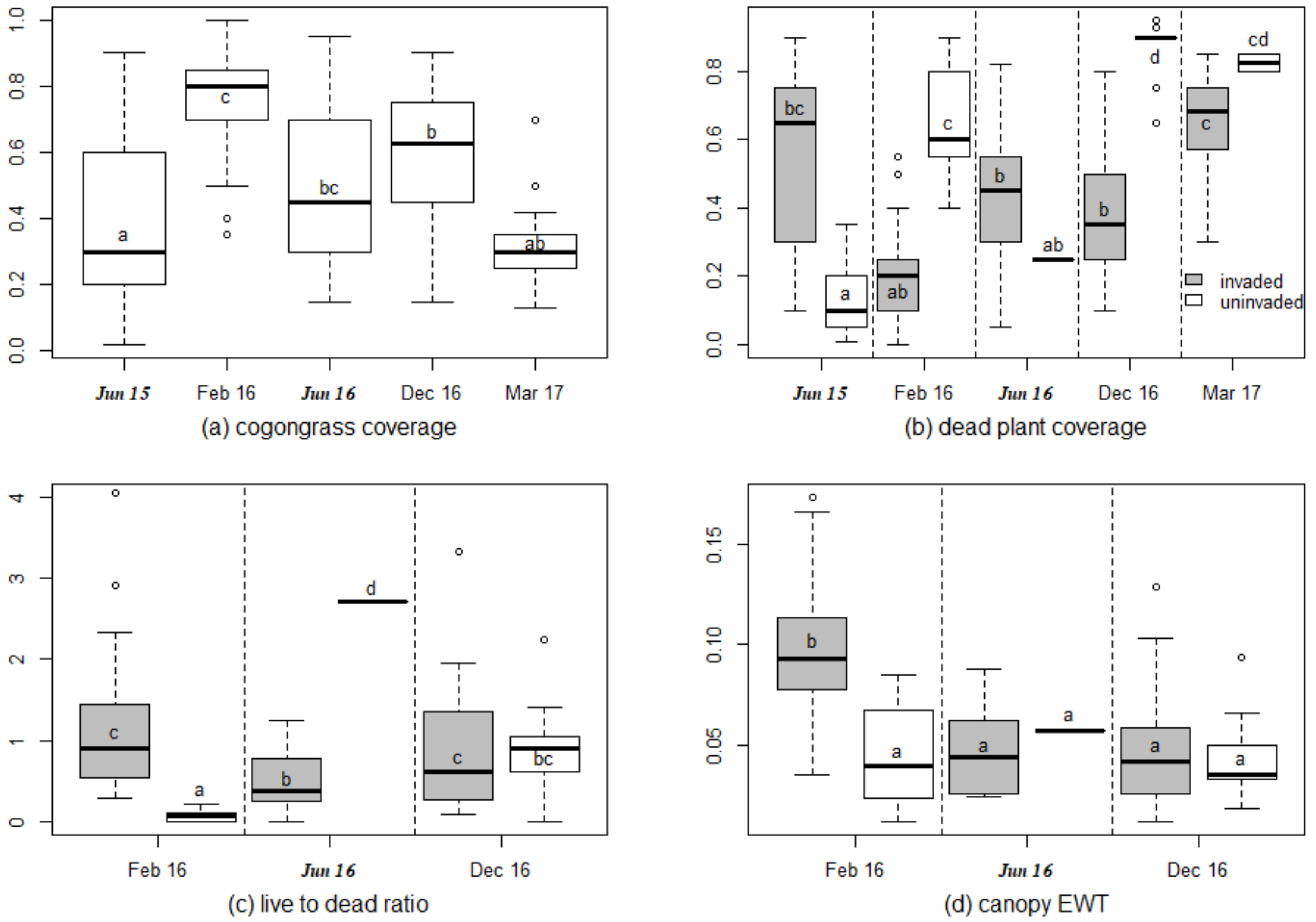
Vegetation characteristics varied among sampling periods, and between invaded and reference treatments (Figure 1, Supplement Table S3). In the invaded subplots, the range of cogongrass coverage was 2% to 100%, and was higher in February 2016, June 2016, and December 2016 than in June 2015 and March 2017 (Figure 1a, p < 0.001). The invaded and uninvaded subplots showed contrasting patterns of dead plant coverage. In dry season periods (February 2016, December 2016, and March 2017), dead plant material coverage was higher in the uninvaded subplots than in the invaded subplots (Figure 1b). In the two wet season periods (June 2015 and June 2016), dead plant material coverage was lower in the uninvaded subplots than in the invaded subplots (p < 0.001, Figure 1b). For canopy water content, the only significant difference between treatments and sampling periods was the significantly higher water content for invaded plots in February 2016 (Figure 1d).
Cogongrass coverage had strong relationships with other vegetation characteristics (Supplement Figure S4). With all of the subplots considered together, higher cogongrass coverage was associated with lower dead plant coverage (r = −0.41), a higher live-to-dead ratio (r = 0.34), and higher canopy EWT (r = 0.49). Among just the invaded subplots, the correlations between cogongrass coverage and other vegetation characteristics were r = −0.94 (dead plant coverage), r = 0.40 (live to dead ratio), and r = 0.49 (canopy EWT).
3.2. Using Spectral Reflectance to Predict Vegetation Characteristics
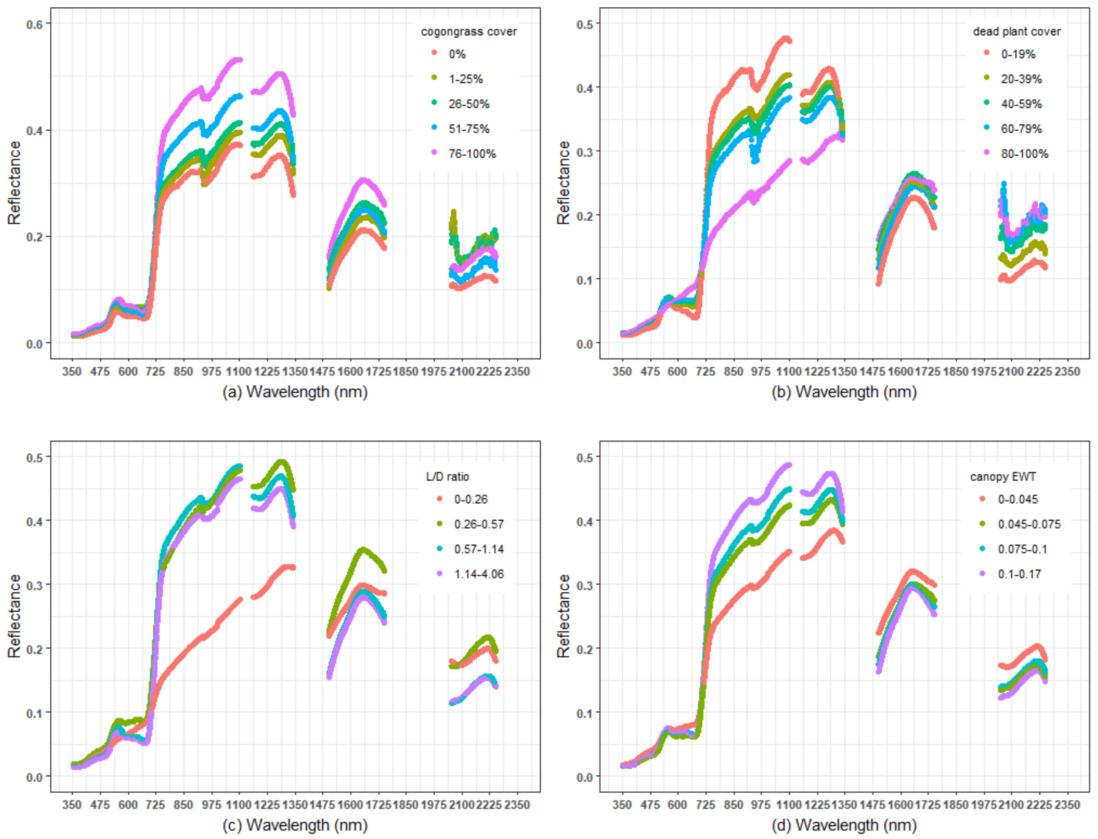
Varying levels of cogongrass coverage, dead plant coverage, and canopy equivalent water thickness (EWT) affected the shape of the spectral curve and the magnitude of reflectance in different wavelength ranges (Figure 2, Supplement Figure S5). High cogongrass cover showed some features that were typical of a large number of vegetation layers, such as high NIR and green reflectance (Figure 2a). However, high cogongrass coverage did not show greater absorption in the red region compared with low cogongrass coverage (Figure 2a). High coverage of dead material showed a pattern typical for non-photosynthetic vegetation (NPV) with low red absorption, low NIR reflectance, and high SWIR reflectance (Figure 2b). Subplots with low canopy EWT showed similar patterns in reflectance as the subplots with a high coverage of dead material (Figure 2b,d).
The PLSR model trained with hyperspectral data collected in the wet season sampling period (June 2015) did not predict the cogongrass or dead plant coverage that was measured in the following year’s wet season sampling period (June 2016) (Table 1 and Table 2, (P) <0 where P = independent validation models using testing data). However, the model trained with data collected in the February 2016 and December 2016 dry seasons predicted the cogongrass coverage ((P) = 0.41) and dead plant coverage ((P) = 0.39) that was measured in the March 2017 dry season. The PLSR model that was trained to predict cogongrass and dead plant coverage from one season (either wet or dry) did not predict cogongrass coverage and dead plant coverage from the other season’s data (dry or wet). The one exception is that the algorithm trained with dead plant coverage data from the dry season predicted dead plant coverage in the wet season ((P) = 0.61). The best prediction with highest and lowest RMSE was achieved when PLSR was trained on a subset of data from all five sampling periods ((P) = 0.68 and 0.57 for cogongrass coverage and dead plant coverage, respectively).
To generate models that are not specific to the season, the PLSR algorithm was trained with two-thirds of the dataset from all of the sampling periods, which were combined to predict the remaining one-third of the data. PLSR models using hyperspectral data produced good estimations for cogongrass coverage ((P) = 0.69) and dead plant coverage ((P) = 0.57), but had a poorer ability to predict canopy EWT ((P) = 0.33) and the live-to-dead plant tissue ratio (P) = −0.08) (Figure 3, Table 3).
The contribution of spectral regions to the PLSR calibration models is revealed by the PLSR regression coefficients, which represent the magnitude and direction that each wavelength has on PLSR factors (Figure 4). The red edge (690–730 nm) and near-infrared (NIR) regions (1000–1050 nm; 1160–1200 nm; 1500–1550 nm) were strong contributors to cogongrass coverage as seen by the large negative and positive coefficient values. For the live-to-dead ratio, the red edge also showed somewhat strong negative coefficients relative to visible and NIR wavelengths. The far-infrared (1200–1300 nm) and SWIR regions (greater than 1600 nm) showed the largest and most negative coefficients. The regression coefficients of both the live-to-dead ratio and canopy EWT were largest around 1240 nm, which is an important wavelength in the normalized difference water index (NDWI), but in opposite directions.
4. Discussion
4.1. Hyperspectral Prediction of Cogongrass Coverage
Hyperspectral data simultaneously predicted invader coverage, dead plant material, and canopy water content in an experimental setting demonstrating that hyperspectral data can be used to non-destructively measure important properties of herbaceous plant communities. However, in order to accurately estimate these properties through time, it is important to have training data from different seasons. We found that PLSR models trained from data measured in one season (either wet or dry) could not predict invader and dead plant coverage from the other season. Similar results were obtained from Yang et al. [23] when examining the leaf traits of several deciduous tree species from northeastern U.S. forests. They found that PLSR models developed from leaf spectral data from one season (winter/summer) could not predict leaf traits in another season (spring/fall). In our study, the inability to predict canopy properties between seasons was likely due to the seasonal changes in leaf traits in both cogongrass and the uninvaded plant species [52]. However, that cogongrass coverage could be quantified when trained with data from both seasons suggests there are characteristics of cogongrass that are distinct from native species, stable between seasons, and can be detected spectrally. For example, cogongrass is high in silica content [24] compared to other species. Furthermore, cogongrass leaf blades are long, tough, and oriented vertically, unlike the co-occurring native plant species.
When trained with data from both the wet and dry seasons, the percent of cogongrass coverage can be estimated well using hyperspectral data and PLSR models. Previously, cogongrass was discriminated successfully from other grass species via hyperspectral data [32]. However, the spectral data used by Mathur et al. [32] was from pure, single-species plots, whereas in many natural systems, cogongrass and other invasive species occur in mixtures with natural vegetation. In this study, we showed that the percent cover of cogongrass, over a wide range of coverages and mixed with other 12 herbaceous species, could be estimated from hyperspectral data. For applications of this method to natural landscapes, cogongrass is most likely to occur both in dense monocultures and mixed with other species, especially where cogongrass is invading new areas. Also, at the scale of airborne and especially satellite images, even pure cogongrass stands will likely be mixed with other vegetation in a single pixel [53], making the detection of cogongrass coverage when it is mixed with other species important.
4.2. Hyperspectral Prediction of Dead Plant Coverage
As expected, we were able to quantify the coverage of dead plant material with hyperspectral data. Dead plant coverage is a critical property to measure in cogongrass-invaded longleaf pine ecosystems, because this invasive species could change the seasonal pattern of dead plant material and enhance fire fuel load. Longleaf pine ecosystems are adapted to frequent, low-intensity fire. Cogongrass can potentially promote more frequent, and/or more intense fires than historically experienced by the ecosystem due to cogongrass’s dense continuous coverage and build-up of dead plant material [28]. The hotter cogongrass-fueled fires can reduce the survival of pine seedlings and the productivity of pine forests [54], and create a positive feedback loop between cogongrass invasion and intense fires [31]. Dead plant coverage could be detected due to reflectance differences between dead plant material and green vegetation in the shape of the green and red bands and the magnitude of reflectance in near-infrared and shortwave-infrared bands. These patterns are consistent with the findings that distinguish green vegetation from non-photosynthetic vegetation (NPV) in airborne AVIRIS data [55]. Other studies have indicated hyperspectral data can quantify dead vegetation [18,56] and fire fuel load [57], of which NPV is an important component [58]. However, NPV can be hard to quantify if landscapes have exposed soil, because NPV and soil are spectrally similar [59]. In the wet season, all of the plots had little soil exposed. In the dry season, especially in uninvaded species plots where most of the vegetation had died, significant amounts of soil were exposed. The differences in exposed soil between seasons may explain why dead plant material could not be predicted in the dry season when the PLSR model was trained in the wet season. Thus, the accurate prediction of NPV may vary seasonally.
4.3. Hyperspectral Detection of Canopy Water Content
Using hyperspectral data and the sampling date, PLSR models predicted canopy EWT, but with higher uncertainties compared to predictions of cogongrass and dead plant material coverage. Other studies have predicted canopy water content from AVIRIS [60], Moderate Resolution Imaging Spectroradiometer (MODIS) [61], and the French Satellite Pour l’Observation de la Terre (SPOT) [62] sensors with greater accuracy than our study. There are several reasons that may explain why our study had a lower than expected predictive ability for canopy EWT. First, the methods and spatial scale at which canopy EWT was measured in the field varies among studies. We directly measured canopy water content in a small column of vegetation within the 0.75 m × 0.75 m measurement footprint. It is more common to estimate canopy EWT indirectly by first measuring the water content of a subsample of leaves, then scaling up the leaf-level water content to the canopy via estimates of leaf area index [62,63,64]. In the more indirect measurements of canopy EWT used in other studies, the hyperspectral signature may be responding to the variables that are used to scale up leaf water content, for example the leaf area index, rather than canopy EWT itself. Furthermore, the small sampling unit of the canopy EWT field measurements in this study may not accurately measure the vertical and horizontal heterogeneity of these understory plant communities. In particular, for the cogongrass plots, the upper part of the dense grass canopy tended to be green, while the lower layers tended to be dead. It is likely that the upper part of the grass canopy had a stronger influence on the spectral signature, whereas our canopy EWT scheme measured water content from the entire vertical profile of the grass canopy. Additional effort to characterize the vertical and horizontal variability in canopy EWT could provide better relationships between reflectance and canopy EWT.
Examining the PLSR regression coefficients weightings can help determine how the spectral regions quantify the vegetation characteristics from both handheld and potentially airborne and satellite hyperspectral sensors. Regions of the near-infrared and shortwave-infrared were important for quantifying cogongrass coverage. Since the structure of cogongrass forms densely packed, vertical grass blades, increasing the coverage of cogongrass led to higher infrared reflectance, which is characteristic of increasing levels of leaf area index [65]. Similar to cogongrass coverage, the near-infrared and shortwave-infrared were important wavelength regions for quantifying dead plant material and canopy water content. In addition, the visible red region between 670–690 nm was important for quantifying dead plant coverage, which could be explained by the chlorophyll content differences between live and dead plants.
4.4. Use of Spectral Data in Experimental Settings—Opportunities and Challenges
Manipulative field experiments are becoming more common in ecology to understand ecosystem level changes in response to climate changes such as increased temperature and drought [33,37,66]. These experiments can provide excellent opportunities to investigate how vegetation change can be detected through remote sensing [66]. In particular, experiments provide a greater control of environmental conditions or species composition than observations or natural systems. In addition, experiments often are accompanied by extensive data collection on vegetation properties and abiotic conditions that can be leveraged in remote sensing studies [37,66]. In our study, the existing long-term experiment allowed us to test the detection of different coverage levels of an invasive species within the context of a fixed pool of uninvaded plant species.
We intended to use hyperspectral data to study the vegetation characteristics in both drought treatments and control plots. However, this approach was not possible, because polycarbonate roofs were used to divert rainfall in the experiment, and light coming through the plastic contaminated the spectral signature of the drought treatment measurements. Thus, in some cases, the equipment that is needed to generate the field-based experimental settings can hinder spectral measurements. If possible, experiments should be designed in such a way to make the spectral measurements of the whole vegetation canopy possible.
4.5. Landscape Scale Detection of Invasive Species
With the PLSR models developed to predict cogongrass coverage and vegetation characteristics, we can now use the spectral data that was collected from the field spectroradiometer to measure invader coverage and vegetation characteristics. At a larger spatial scale than the experimental plots, remote sensing methods can be used to map and monitor invasive species at landscape levels. Our study supports that cogongrass coverage should be detectable from airborne or satellite hyperspectral sensors where cogongrass is invading pastures and natural systems, particularly open longleaf pine savannas. The increasing availability of airborne hyperspectral data, such as for example from campaigns associated with the National Ecological Observatory Network in the U.S. and the Terrestrial Ecosystem Research Network in Australia, new satellite hyperspectral sensors, such as HyspIRI [67] and Enmap [67], and hyperspectral sensors carried by unmanned aerial vehicles [68,69], provide important data sources for mapping this invasive species. This study suggests that spectral regions, especially red-edge, near-infrared and shortwave-infrared regions, may be important for the landscape-scale mapping of cogongrass. These wavelength regions are covered by multi-spectral satellite sensors as well, such as Sentinel 2 and Worldview-3, which may allow for the mapping of cogongrass from these platforms. The large-scale mapping of the coverage of cogongrass and other plant invaders is important for detecting important ecosystem consequences driven by plant invasion, such as the seasonal build-up of dead plant material, the alteration of vegetation water content, and changes to fire fuel loads, which should be possible using hyperspectral data. Taking into account the seasonal dynamics of invaded ecosystems is critical for the quantitative mapping of invaders and their impacts.
5. Conclusions
Our study showed that partial least square regression models (PLSR) applied to hyperspectral data can estimate cogongrass coverage, dead plant coverage, and canopy equivalent water thickness (EWT) in a common garden experiment in which the presence of invasive species, the matrix of co-occurring species, and environmental conditions are controlled. Capturing the seasonality of the invasive cogongrass and co-occurring vegetation within the training dataset was important for developing robust models that predict invasive plant cover and its impacts within and between years. The need to use spectral data from different seasons to build robust models that estimate invasive plant coverage is likely to be a widespread phenomenon, given that invasives often have different seasonal patterns than co-occurring plants, and alter the seasonal patterns of ecosystems properties [23]. The results developed in this small-scale experimental setting provides guidance for the large-scale quantification of cogongrass and its effects on diverse longleaf pine ecosystems using airborne imaging spectrometers. The near-infrared and shortwave-infrared spectral regions had strong weightings in the PLSR models of cogongrass coverage and vegetation characteristics, suggesting an emphasis on data collection and analyses in these wavelength regions to estimate cogongrass coverage from airborne or satellite-based hyperspectral systems. More generally, the use of experimental, small-scale plots to understand ways to develop robust models (e.g., key wavelength regions, seasonal patterns) may provide information on how to deploy and use large-scale hyperspectral image data to map the important ecological features of landscapes.
Supplementary Materials
The following are available online at https://www.mdpi.com/2072-4292/10/5/784/s1, Figure S1: Coefficient of determination (R2) of Partial Least Square Regression (PLSR) using field spectral data to predict (a) cogongrass and (b) dead plant coverage using training sets of different sizes, Figure S2: Reflectance of 10 subplots randomly selected from (a) ambient invaded subplots, (b) ambient uninvaded subplots, (c) drought invaded subplots, and (d) drought uninvaded subplots, Figure S3: The results of PLSR models for cogongrass coverage, dead plant coverage, live to dead plant material ratio, and canopy EWT using original reflectance from drought dataset, Figure S4: Pearson correlation between the vegetation characteristics under ambient treatment, Figure S5: Mean hyperspectral reflectance in just the visible wavelength ranges for different quantiles of the following vegetation characteristics: (a) cogongrass coverage, (b) dead plant coverage, (c) live to dead plant material ratio, and (d) canopy EWT, Table S1: The number of plant samples in each field campaign, Table S2: Predictive ability of hyperspectral estimation of vegetation characteristics using data from drought plots, Table S3: The results from a nonparametric analysis of variance (Kruskal-Wallis test) for sampling period, cogongrass introduction, and their interaction among experimental subplots in (a) cogongrass coverage, (b) dead plant coverage, (c) live to dead plant material ratio, and (d) canopy EWT.
Author Contributions
S.B., S.L.F., Y.G and S.G. conceived and designed the experiments; S.G., S.B. and Y.G. performed the experiments; Y.G. and S.B. analyzed the data; Y.G. and S.B. wrote the paper.
Acknowledgments
Aidan McCormick, Christine Swanson, Drew Hiatt, Anbinh Ho, Hannah Borchelt, and Yuan Zhou helped collect field data. Catherine Fahey provided the plant cover estimates. SLF was funded by the University of Florida, Institute of Food and Agricultural Sciences (UF/IFAS); the Florida Forest Service, Florida Department of Agriculture and Consumer Services (Contract#21942); and the USDA/NIFA McIntire-Stennis program (FLA-AGR-005180). SAB was funded by the Institute of Food and Agricultural Sciences (UF/IFAS) and the USDA/NIFA McIntire-Stennis program (FLA-FOR-005470).
Conflicts of Interest
The authors declare no conflicts of interest.
References
- Brook, R.M. Review of literature on Imperata cylindrica (L.) Raeuschel with particular reference to South East Asia. Int. J. Pest Manag. 1989, 35, 12–25. [Google Scholar]
- Martin, H.; Petr, P.; Vojtěch, J. Impact of invasive plants on the species richness, diversity and composition of invaded communities. J. Ecol. 2009, 97, 393–403. [Google Scholar] [CrossRef]
- Barnes, T.G.; DeMaso, S.J.; Bahm, M.A. The Impact of 3 exotic, invasive grasses in the Southeastern United States on wildlife. Wildland Soc. Bull. 2013, 37, 497–502. [Google Scholar] [CrossRef]
- Davies, K.W.; Nafus, A.M. Exotic annual grass invasion alters fuel amounts, continuity and moisture content. Int. J. Wildland Fire 2013, 22, 353–358. [Google Scholar] [CrossRef]
- Shaw, D.R. Translation of remote sensing data into weed management decisions. Weed Sci. 2005, 53, 264–273. [Google Scholar] [CrossRef]
- He, K.S.; Rocchini, D.; Neteler, M.; Nagendra, H. Benefits of hyperspectral remote sensing for tracking plant invasions. Div. Distrib. 2011, 17, 381–392. [Google Scholar] [CrossRef]
- Peterson, E.B. Estimating cover of an invasive grass (Bromus tectorum) using tobit regression and phenology derived from two dates of Landsat ETM+ data. Int. J. Remote Sens. 2005, 26, 2491–2507. [Google Scholar] [CrossRef]
- Asner, G.P.; Knapp, D.E.; Kennedy-Bowdoin, T.; Jones, M.O.; Martin, R.E.; Boardman, J.; Hughes, R.F. Invasive species detection in Hawaiian rainforests using airborne imaging spectroscopy and LiDAR. Remote Sens. Environ. 2008, 112, 1942–1955. [Google Scholar] [CrossRef]
- Richardson, A.D.; Braswell, B.H.; Hollinger, D.Y.; Jenkins, J.P.; Ollinger, S.V. Near-surface remote sensing of spatial and temporal variation in canopy phenology. Ecol. Appl. 2009, 19, 1417–1428. [Google Scholar] [CrossRef] [PubMed]
- Asner, G.P.; Vitousek, P.M. Remote analysis of biological invasion and biogeochemical change. Proc. Natl. Acad. Sci. USA 2005, 102, 4383–4386. [Google Scholar] [CrossRef] [PubMed]
- Schlerf, M.; Atzberger, C.; Hill, J. Remote sensing of forest biophysical variables using HyMap imaging spectrometer data. Remote Sens. Environ. 2005, 95, 177–194. [Google Scholar] [CrossRef]
- Huang, C.; Asner, G.P. Applications of Remote Sensing to Alien Invasive Plant Studies. Sensors 2009, 9, 4869–4889. [Google Scholar] [CrossRef] [PubMed]
- Schmidt, K.S.; Skidmore, A.K. Spectral discrimination of vegetation types in a coastal wetland. Remote Sens. Environ. 2003, 85, 92–108. [Google Scholar] [CrossRef]
- Asner, G.P.; Martin, R.E.; Anderson, C.B.; Knapp, D.E. Quantifying forest canopy traits: Imaging spectroscopy versus field survey. Remote Sens. Environ. 2015, 158, 15–27. [Google Scholar] [CrossRef]
- Underwood, E.; Ustin, S.; DiPietro, D. Mapping nonnative plants using hyperspectral imagery. Remote Sens. Environ. 2003, 86, 150–161. [Google Scholar] [CrossRef]
- Hunt, E.R.; McMurtrey, J.E.; Parker Williams, A.E.; Corp, L.A. Spectral characteristics of leafy spurge (Euphorbia esula) leaves and flower bracts. Weed Sci. 2004, 52, 492–497. [Google Scholar] [CrossRef]
- Hestir, E.L.; Khanna, S.; Andrew, M.E.; Santos, M.J.; Viers, J.H.; Greenberg, J.A.; Rajapakse, S.S.; Ustin, S.L. Identification of invasive vegetation using hyperspectral remote sensing in the California Delta ecosystem. Remote Sens. Environ. 2008, 112, 4034–4047. [Google Scholar] [CrossRef]
- Varga, T.A.; Asner, G.P. Hyperspectral and lidar remote sensing of fire fuels in hawaii volcanoes national park. Ecol. Appl. 2008, 18, 613–623. [Google Scholar] [CrossRef] [PubMed]
- Olsson, A.D.; van Leeuwen, W.J.D.; Marsh, S.E. Feasibility of Invasive Grass Detection in a Desertscrub Community Using Hyperspectral Field Measurements and Landsat TM Imagery. Remote Sens. 2011, 3, 2283–2304. [Google Scholar] [CrossRef]
- Ishii, J.; Washitani, I. Early detection of the invasive alien plant Solidago altissima in moist tall grassland using hyperspectral imagery. Int. J. Remote Sens. 2013, 34, 5926–5936. [Google Scholar] [CrossRef]
- Barbosa, J.M.; Asner, G.P.; Martin, R.E.; Baldeck, C.A.; Hughes, F.; Johnson, T. Determining Subcanopy Psidium cattleianum Invasion in Hawaiian Forests Using Imaging Spectroscopy. Remote Sens. 2016, 8, 33. [Google Scholar] [CrossRef]
- Noujdina, N.V.; Ustin, S.L. Mapping Downy Brome (Bromus tectorum) Using Multidate AVIRIS Data. Weed Sci. 2008, 56, 173–179. [Google Scholar] [CrossRef]
- Yang, X.; Tang, J.; Mustard, J.F.; Wu, J.; Zhao, K.; Serbin, S.; Lee, J.-E. Seasonal variability of multiple leaf traits captured by leaf spectroscopy at two temperate deciduous forests. Remote Sens. Environ. 2016, 179, 1–12. [Google Scholar] [CrossRef]
- Dozier, H.; Gaffney, J.F.; McDonald, S.K.; Johnson, E.R.R.L.; Shilling, D.G. Cogongrass in the United States: History, Ecology, Impacts, and Management. Weed Technol. 1998, 12, 737–743. [Google Scholar] [CrossRef]
- Lippincott, C.L. Ecological consequences of Imperata cylindrica (cogongrass) invasion in Florida sandhill. Doctoral Dissertation, University of Florida, Gainesville, FL, USA, 1997. [Google Scholar]
- Brewer, S. Declines in plant species richness and endemic plant species in longleaf pine savannas invaded by Imperata cylindrica. Biol. Invasions 2008, 10, 1257–1264. [Google Scholar] [CrossRef]
- MacDonald, G.E. Cogongrass (Imperata cylindrical)—Biology, ecology, and management. Crit. Rev. Plant Sci. 2004, 23, 367–380. [Google Scholar] [CrossRef]
- Tominaga, T. Seasonal change in the standing crop of Imperata cylindrical var. koenigii grassland in the Kii-Oshima Island of Japan. Weed Res. Jpn. 1989, 34, 127–132. [Google Scholar]
- Estrada, J.A.; Flory, S.L. Cogongrass (Imperata cylindrica) invasions in the US: Mechanisms, impacts, and threats to biodiversity. Glob. Ecol. Conserv. 2015, 3, 1–10. [Google Scholar] [CrossRef]
- Lippincott, C.L. Effects of Imperata cylindrical (L.) Beauv. (Cogongrass) Invasion on Fire Regime in Florida Sandhill (USA). Nat. Areas J. 2000, 20, 140–149. [Google Scholar]
- King, S.E.; Grace, J.B. The effects of gap size and disturbance type on invasion of wet pine savanna by cogongrass, Imperata cylindrica (Poaceae). Am. J. Bot. 2000, 87, 1279–1286. [Google Scholar] [CrossRef] [PubMed]
- Mathur, A.; Bruce, L.M.; Byrd, J. Discrimination of subtly different vegetative species via hyperspectral data. In Proceedings of the IEEE International on Geoscience and Remote Sensing Symposium, Toronto, ON, Canada, 24–28 June 2002; Volume 2, pp. 805–807. [Google Scholar]
- Huang, Y.; Bruce, L.M.; Byrd, J.; Mask, B. Using wavelet transform of hyperspectral reflectance curves for automated monitoring of Imperata cylindrica (cogongrass). In Proceedings of the IEEE 2001 International on Geoscience and Remote Sensing Symposium (Cat. No.01CH37217, Sydney, NSW, Australia, 9–13 July 2001; Volume 5, pp. 2244–2246. [Google Scholar]
- Peet, R.K.; Allard, D.J. Longleaf pine vegetation of the southern Atlantic and eastern Gulf Coast regions: A preliminary classification. In Proceedings of the Tall Timbers Fire Ecology Conference; Tall Timbers Research Station: Tallahassee, FL, USA, 1993; Volume 18, pp. 45–81. [Google Scholar]
- Rocchini, D.; Balkenhol, N.; Carter, G.A.; Foody, G.M.; Gillespie, T.W.; He, K.S.; Kark, S.; Levin, N.; Lucas, K.; Luoto, M. Remotely sensed spectral heterogeneity as a proxy of species diversity: Recent advances and open challenges. Ecol. Inform. 2010, 5, 318–329. [Google Scholar] [CrossRef]
- Heumann, B.W.; Hackett, R.A.; Monfils, A.K. Testing the spectral diversity hypothesis using spectroscopy data in a simulated wetland community. Ecol. Inform. 2015, 25, 29–34. [Google Scholar] [CrossRef]
- Alba, C.; NeSmith, J.E.; Fahey, C.; Angelini, C.; Flory, S.L. Methods to test the interactive effects of drought and plant invasion on ecosystem structure and function using complementary common garden and field experiments. Ecol. Evol. 2017, 7, 1442–1452. [Google Scholar] [CrossRef] [PubMed]
- Underwood, E.C.; Mulitsch, M.J.; Greenberg, J.A.; Whiting, M.L.; Ustin, S.L.; Kefauver, S.C. Mapping Invasive Aquatic Vegetation in the Sacramento-San Joaquin Delta using Hyperspectral Imagery. Environ. Monit. Assess. 2006, 121, 47–64. [Google Scholar] [CrossRef] [PubMed]
- Fahey, C.; Angellini, C.; Flory, S. Grass invasion and drought interact to alter the diversity and structure of native plant communities. 2018; in press. [Google Scholar]
- Danson, F.M.; Steven, M.D.; Malthus, T.J.; Clark, J.A. High-spectral resolution data for determining leaf water content. Int. J. Remote Sens. 1992, 13, 461–470. [Google Scholar] [CrossRef]
- Kruskal, W.H.; Wallis, W.A. Use of ranks in one-criterion variance analysis. J. Am. Stat. Assoc. 1952, 47, 583–621. [Google Scholar] [CrossRef]
- Dunn, O.J. Multiple comparisons using rank sums. Technometrics 1964, 6, 241–252. [Google Scholar] [CrossRef]
- Wold, S.; Sjöström, M.; Eriksson, L. PLS-regression: A basic tool of chemometrics. Chemom. Intell. Lab. Syst. 2001, 58, 109–130. [Google Scholar] [CrossRef]
- Kennard, R.W.; Stone, L.A. Computer Aided Design of Experiments. Technometrics 1969, 11, 137–148. [Google Scholar] [CrossRef]
- Miles, J. R Squared, Adjusted R Squared. Wiley StatsRef Stat. Ref. Online 2014. [Google Scholar] [CrossRef]
- RS Team. RStudio: Integrated Development for R; RStudio Inc.: Boston, MA, USA, 2015. [Google Scholar]
- Wehrens, R.; Mevik, B.H. The pls package: Principal component and partial least squares regression in R. J. Stat. Softw. 2007, 18, 1–24. [Google Scholar]
- Stevens, A.; Ramirez–Lopez, L. An Introduction to the Prospectr Package. Available online: ftp://200.236.31.2/CRAN/web/packages/prospectr/vignettes/prospectr-intro.pdf (accessed on 14 February 2014).
- Gao, B. NDWI—A normalized difference water index for remote sensing of vegetation liquid water from space. Remote Sens. Environ. 1996, 58, 257–266. [Google Scholar] [CrossRef]
- Hardisky, M.A.; Klemas, V.; Smart, M. The influence of soil salinity, growth form, and leaf moisture on the spectral radiance of. Spartina Alterniflora 1983, 49, 77–83. [Google Scholar]
- Rouse, J., Jr.; Haas, R.H.; Schell, J.A.; Deering, D.W. Monitoring Vegetation Systems in the Great Plains with ERTS; NASA: College Station, TX, USA, 1974; Volume 1, pp. 309–317. [Google Scholar]
- Fajardo, A.; Siefert, A. Phenological variation of leaf functional traits within species. Oecologia 2016, 180, 951–959. [Google Scholar] [CrossRef] [PubMed]
- Ichoku, C.; Karnieli, A. A review of mixture modeling techniques for sub-pixel land cover estimation. Remote Sens. Rev. 1996, 13, 161–186. [Google Scholar] [CrossRef]
- Daneshgar, P.; Jose, S.; Collins, A.; Ramsey, C. Cogongrass (Imperata cylindrica), an alien invasive grass, reduces survival and productivity of an establishing pine forest. For. Sci. 2008, 54, 579–587. [Google Scholar]
- Roberts, D.A.; Smith, M.O.; Adams, J.B. Green vegetation, nonphotosynthetic vegetation, and soils in AVIRIS data. Remote Sens. Environ. 1993, 44, 255–269. [Google Scholar] [CrossRef]
- Guerschman, J.P.; Hill, M.J.; Renzullo, L.J.; Barrett, D.J.; Marks, A.S.; Botha, E.J. Estimating fractional cover of photosynthetic vegetation, non-photosynthetic vegetation and bare soil in the Australian tropical savanna region upscaling the EO-1 Hyperion and MODIS sensors. Remote Sens. Environ. 2009, 113, 928–945. [Google Scholar] [CrossRef]
- Mutlu, M.; Popescu, S.C.; Zhao, K. Sensitivity analysis of fire behavior modeling with LIDAR-derived surface fuel maps. For. Ecol. Manag. 2008, 256, 289–294. [Google Scholar] [CrossRef]
- Chuvieco, E.; Aguado, I.; Dimitrakopoulos, A.P. Conversion of fuel moisture content values to ignition potential for integrated fire danger assessment. Can. J. For. Res. 2004, 34, 2284–2293. [Google Scholar] [CrossRef]
- Okin, G.S. Relative spectral mixture analysis—A multitemporal index of total vegetation cover. Remote Sens. Environ. 2007, 106, 467–479. [Google Scholar] [CrossRef]
- Serrano, L.; Ustin, S.L.; Roberts, D.A.; Gamon, J.A.; Peñuelas, J. Deriving Water Content of Chaparral Vegetation from AVIRIS Data. Remote Sens. Environ. 2000, 74, 570–581. [Google Scholar] [CrossRef]
- Cheng, Y.-B.; Ustin, S.L.; Riaño, D.; Vanderbilt, V.C. Water content estimation from hyperspectral images and MODIS indexes in Southeastern Arizona. Remote Sens. Environ. 2008, 112, 363–374. [Google Scholar] [CrossRef]
- Ceccato, P.; Gobron, N.; Flasse, S.; Pinty, B.; Tarantola, S. Designing a spectral index to estimate vegetation water content from remote sensing data: Part 1: Theoretical approach. Remote Sens. Environ. 2002, 82, 188–197. [Google Scholar] [CrossRef]
- Colombo, R.; Meroni, M.; Marchesi, A.; Busetto, L.; Rossini, M.; Giardino, C.; Panigada, C. Estimation of leaf and canopy water content in poplar plantations by means of hyperspectral indices and inverse modeling. Remote Sens. Environ. 2008, 112, 1820–1834. [Google Scholar] [CrossRef]
- Yilmaz, M.T.; Hunt, E.R.; Jackson, T.J. Remote sensing of vegetation water content from equivalent water thickness using satellite imagery. Remote Sens. Environ. 2008, 112, 2514–2522. [Google Scholar] [CrossRef]
- Price, J.C.; Bausch, W.C. Leaf area index estimation from visible and near-infrared reflectance data. Remote Sens. Environ. 1995, 52, 55–65. [Google Scholar] [CrossRef]
- Asner, G.P.; Nepstad, D.; Cardinot, G.; Ray, D. Drought stress and carbon uptake in an Amazon forest measured with spaceborne imaging spectroscopy. Proc. Natl. Acad. Sci. USA 2004, 101, 6039–6044. [Google Scholar] [CrossRef] [PubMed]
- Lee, C.M.; Cable, M.L.; Hook, S.J.; Green, R.O.; Ustin, S.L.; Mandl, D.J.; Middleton, E.M. An introduction to the NASA Hyperspectral InfraRed Imager (HyspIRI) mission and preparatory activities. Remote Sens. Environ. 2015, 167, 6–19. [Google Scholar] [CrossRef]
- Dvorák, P.; Müllerová, J.; Bartalos, T.; Bruna, J. Unmanned Aerial Vehicles for Alien Plant Species Detection and Monitoring. In The International Archives of Photogrammetry, Remote Sensing and Spatial Information Sciences; Copernicus GmbH: Göttingen, Germany, 2015; Volume XL, pp. 83–90. [Google Scholar]
- Hill, D.J.; Tarasoff, C.; Whitworth, G.E.; Baron, J.; Bradshaw, J.L.; Church, J.S. Utility of unmanned aerial vehicles for mapping invasive plant species: A case study on yellow flag iris (Iris pseudacorus L.). Int. J. Remote Sens. 2017, 38, 2083–2105. [Google Scholar] [CrossRef]
Figure 1.
Box plots showing the following vegetation characteristics in ambient (non-drought) subplots for uninvaded and cogongrass-invaded subplots through time: (a) cogongrass coverage, (b) dead plant coverage, (c) live-to-dead material ratio, and (d) canopy equivalent water thickness (EWT). On the x-axis, the sample periods from the wet season are in bold and italics. For figure (a), the cogongrass coverage for the uninvaded subplots in all of the sampling periods is zero. Data ranking was implemented by the Kruskal–Wallis test. Small letters denote statistical significance of Dunn’s post hoc multiple comparisons among treatments.

Figure 2.
Mean hyperspectral reflectance for different quantiles of the following vegetation characteristics: (a) cogongrass coverage, (b) dead plant coverage, (c) live-to-dead ratio, and (d) canopy equivalent water thickness (EWT) for the full spectral range. Data were combined from all of the sampling periods.

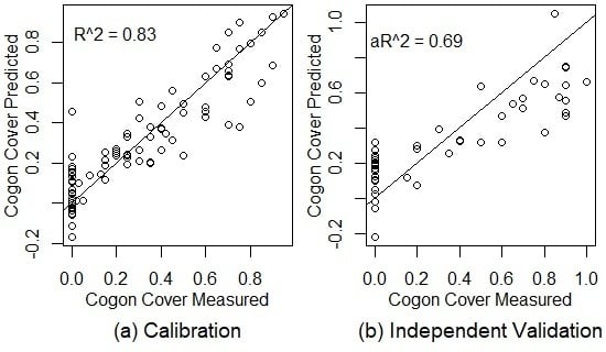
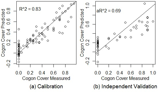
Figure 3.
The results of PLSR models for cogongrass coverage, dead plant coverage, the live-to-dead ratio, and canopy EWT with training and testing data drawn from all of the dates combined for calibration (a) and independent validation (b). The black lines are 1:1 lines. = coefficient of determination, a = adjusted coefficient of determination. EWT = equivalent water thickness.

Figure 4.
The PLSR model regression coefficients plotted by wavelength for four variables: cogongrass cover (a), dead plot cover (b), live-to-dead ratio (c), and canopy equivalent water thickness (EWT) (d). The wavelength center of water band index (WBI) in red, normalized difference water index (NDWI) in yellow [49], normalized difference infrared index (NDII) in blue [50], and normalized difference vegetation index (NDVI) in green [51] are presented as the vertical lines as references.


Table 1.
Performance of partial least square regression (PLSR) reflectance models on cogongrass coverage that were calibrated and validated using data from different sampling periods. NL = number of latent variables; RMSE = root mean square error; C = calibration models using training data; P = independent validation models using testing data.
| Training Data | Test Data | Results | |||||||
|---|---|---|---|---|---|---|---|---|---|
| Season (Date) | Sample Size | Season (Date) | Sample Size | NL | R2 (C) | RMSE (C) | (P) | RMSE (P) | |
| Same Season | wet (6/2015) | 54 | wet (6/2016) | 10 | 7 | 0.88 | 0.09 | −0.88 | 0.42 |
| dry (2/2016 + 12/2016) | 57 | dry (3/2017) | 16 | 4 | 0.85 | 0.14 | 0.41 | 0.13 | |
| Different Season | wet (6/2015 + 6/2016) | 56 | dry (2/2016 + 12/2016 + 3/2017) | 28 | 11 | 0.89 | 0.09 | −6.59 | 0.8 |
| dry (2/2016 + 12/2016 + 3/2017) | 56 | wet (6/2015 + 6/2016) | 28 | 10 | 0.93 | 0.08 | −1.80 | 0.5 | |
| All Seasons Together | wet and dry (6/2015 + 2/2016 + 6/2016 + 12/2016 + 3/2017) | 91 | wet and dry (6/2015 + 2/2016 + 6/2016 + 12/2016 + 3/2017) | 46 | 11 | 0.83 | 0.12 | 0.68 | 0.21 |
Table 2.
Performance of PLSR reflectance models on dead plant coverage that were calibrated and validated using data from different sampling periods. NL = number of latent variables; RMSE = root mean square error; C = calibration models using training data; P = independent validation models using testing data.
| Training Data | Test Data | Results | |||||||
|---|---|---|---|---|---|---|---|---|---|
| Season (Date) | Sample Size | Season (Date) | Sample Size | NL | R2 (C) | RMSE (C) | (P) | RMSE (P) | |
| Same Season | wet (6/2015) | 54 | wet (6/2016) | 10 | 7 | 0.91 | 0.09 | −1.21 | 0.34 |
| dry (2/2016 + 12/2016) | 57 | dry (3/2017) | 16 | 4 | 0.79 | 0.14 | 0.43 | 0.11 | |
| Different Season | wet (6/2015 + 6/2016) | 56 | dry (2/2016 + 12/2016 + 3/2017) | 28 | 9 | 0.87 | 0.1 | −2.27 | 0.49 |
| dry (2/2016 + 12/2016 + 3/2017) | 56 | wet (6/2015 + 6/2016) | 28 | 9 | 0.91 | 0.09 | 0.61 | 0.17 | |
| All Seasons Together | wet and dry (6/2015 + 2/2016 + 6/2016 + 12/2016 + 3/2017) | 91 | wet and dry (6/2015 + 2/2016 + 6/2016 + 12/2016 + 3/2017) | 46 | 9 | 0.87 | 0.11 | 0.57 | 0.16 |
Table 3.
Predictive ability of hyperspectral estimation of vegetation characteristics in an experimental setting. The training and testing data were taken from a combined data set from all of the sampling periods where each vegetation characteristic was measured. EWT = canopy equivalent water thickness; NL = number of latent variables; RMSE = root mean square error; RE = relative error; C = calibration models using training data; CV = cross-validation models using leave one out; P = independent validation models using testing data; L/D: live-to-dead ratio.
| Vegetation Characteristic | NL | R2 (C) | RMSE (C) | RE (C) | R2 (CV) | RMSE (CV) | RE (CV) | (P) | RMSE (P) | RE (P) |
|---|---|---|---|---|---|---|---|---|---|---|
| Cogon Cover | 11 | 0.83 | 0.123 | 39.78% | 0.65 | 0.196 | 59.50% | 0.69 | 0.206 | 55.99% |
| Dead Plant | 9 | 0.87 | 0.105 | 20.91% | 0.74 | 0.151 | 35.49% | 0.57 | 0.155 | 57.01% |
| L/D Ratio | 3 | 0.23 | 1.095 | 111.64% | 0.10 | 1.048 | 107.81% | −0.08 | 0.712 | 74.45% |
| Canopy EWT | 5 | 0.45 | 0.025 | 43.75% | 0.28 | 0.032 | 51.22% | 0.33 | 0.033 | 44.94% |
© 2018 by the authors. Licensee MDPI, Basel, Switzerland. This article is an open access article distributed under the terms and conditions of the Creative Commons Attribution (CC BY) license (http://creativecommons.org/licenses/by/4.0/).
Share and Cite
MDPI and ACS Style
Guo, Y.; Graves, S.; Flory, S.L.; Bohlman, S. Hyperspectral Measurement of Seasonal Variation in the Coverage and Impacts of an Invasive Grass in an Experimental Setting. Remote Sens. 2018, 10, 784. https://doi.org/10.3390/rs10050784
AMA Style
Guo Y, Graves S, Flory SL, Bohlman S. Hyperspectral Measurement of Seasonal Variation in the Coverage and Impacts of an Invasive Grass in an Experimental Setting. Remote Sensing. 2018; 10(5):784. https://doi.org/10.3390/rs10050784
Chicago/Turabian StyleGuo, Yuxi, Sarah Graves, S. Luke Flory, and Stephanie Bohlman. 2018. "Hyperspectral Measurement of Seasonal Variation in the Coverage and Impacts of an Invasive Grass in an Experimental Setting" Remote Sensing 10, no. 5: 784. https://doi.org/10.3390/rs10050784
Note that from the first issue of 2016, this journal uses article numbers instead of page numbers. See further details here.