SAR-Based Estimation of Above-Ground Biomass and Its Changes in Tropical Forests of Kalimantan Using L- and C-Band

1
Remote Sensing Solutions GmbH, Isarstr. 3, 82065 Baierbrunn, Germany
2
Department of Biology, Ludwig-Maximilians-University Munich, Großhaderner Str. 2, 82152 Planegg-Martinsried, Germany
*
Author to whom correspondence should be addressed.
Remote Sens. 2018, 10(6), 831; https://doi.org/10.3390/rs10060831
Submission received: 6 April 2018
/
Revised: 18 May 2018
/
Accepted: 24 May 2018
/
Published: 25 May 2018
(This article belongs to the Special Issue Remote Sensing of Forest Cover Change)
Abstract
:Kalimantan poses one of the highest carbon emissions worldwide since its landscape is strongly endangered by deforestation and degradation and, thus, carbon release. The goal of this study is to conduct large-scale monitoring of above-ground biomass (AGB) from space and create more accurate biomass maps of Kalimantan than currently available. AGB was estimated for 2007, 2009, and 2016 in order to give an overview of ongoing forest loss and to estimate changes between the three time steps in a more precise manner. Extensive field inventory and LiDAR data were used as reference AGB. A multivariate linear regression model (MLR) based on backscatter values, ratios, and Haralick textures derived from Sentinel-1 (C-band), ALOS PALSAR (Advanced Land Observing Satellite’s Phased Array-type L-band Synthetic Aperture Radar), and ALOS-2 PALSAR-2 polarizations was used to estimate AGB across the country. The selection of the most suitable model parameters was accomplished considering VIF (variable inflation factor), p-value, R2, and RMSE (root mean square error). The final AGB maps were validated by calculating bias, RMSE, R2, and NSE (Nash-Sutcliffe efficiency). The results show a correlation (R2) between the reference biomass and the estimated biomass varying from 0.69 in 2016 to 0.77 in 2007, and a model performance (NSE) in a range of 0.70 in 2016 to 0.76 in 2007. Modelling three different years with a consistent method allows a more accurate estimation of the change than using available biomass maps based on different models. All final biomass products have a resolution of 100 m, which is much finer than other existing maps of this region (>500 m). These high-resolution maps enable identification of even small-scaled biomass variability and changes and can be used for more precise carbon modelling, as well as forest monitoring or risk managing systems under REDD+ (Reducing Emissions from Deforestation, forest Degradation, and the role of conservation, sustainable management of forests, and enhancement of forest carbon stocks) and other programs, protecting forests and analyzing carbon release.
1. Introduction
The Earth’s land surface spans approximately 149.4 million km2, of which nearly 30% is characterized by forested areas [1]. Tropical forest ecosystems (forests and soils) alone hold about 40% of terrestrial carbon [2,3]. However, due to unsustainable use and deforestation, the stored carbon can be released into the atmosphere as CO2 (carbon dioxide) and will contribute significantly to global climate change. According to the Intergovernmental Panel on Climate Change (IPCC), the resulting greenhouse gas emissions account for approximately 11% of all anthropogenic emissions worldwide [4,5].
The forests of Indonesia are considered to be one of the oldest and most species-rich tropical rainforests on the planet [6]. Indonesia’s forests alone store 18.6 Gt of carbon [7]. Additionally, the country has some of the largest known tropical peat reservoirs on Earth, storing 55–58 Gt of carbon in belowground peatlands ([8,9]). At the same time the deforestation and degradation of these tropical ecosystems lead to a considerable release of carbon, making Indonesia, especially Kalimantan and Sumatra, one of the largest carbon emitters worldwide [10]. Digging canals for means of transport is a detrimental form of degradation, as it causes drying in peatlands and encourages the spread of fires and, thus, increases the potential of forest and peatland loss. As a result of the significant emission levels and immense loss of forests and peatlands, Indonesia has become a prime target for REDD+ projects (Reducing Emissions from Deforestation, forest Degradation, and the role of conservation, sustainable management of forests, and enhancement of forest carbon stocks). One of the intentions of REDD+ includes conditional payments to developing countries for reducing their emissions [11]. Within this framework, the most active projects and initiatives worldwide are taking place in Indonesia and its provinces [12]. Nevertheless, Indonesia, especially Kalimantan, the largest isle of Indonesia, is affected by ongoing deforestation and degradation processes.
To perform current REDD+ policies, accurate forest monitoring systems, consistent measurements, and information about carbon emissions at national and subnational scales are necessary for participating countries. Especially, subnational projects require accurate high-resolution maps capturing small-scaled variability and changes in forested areas. Forest carbon stocks are usually calculated using above-ground biomass (AGB) by assuming that typically 50% of AGB is carbon [13]. Biomass, as the fundamental biophysical parameter quantifying the Earth’s living vegetation [14], describes the amount of woody matter within a forest. It is defined by the Global Climate Observing System (GCOS) as an essential climate variable (ECV) [15]. Well-known methods for mapping AGB include field-data, airborne and space-borne LiDAR (light detection and ranging) scanning, satellite optical remote sensing, and imaging radar [14]. In contrast to ground-based inventories and LiDAR surveys, Earth observation approaches are able to cover larger areas and in a more cost-effective manner. Additionally, forest inventories are not always comparable, since the definition of national forests and sampling strategies vary between countries [16].
An appropriate compromise represents the upscaling of accurate forest inventories or regional LiDAR-derived biomass estimations with large-scale satellite imagery [17]. Since optical data are limited by clouds, smoke, and lacking illumination, as well as not being able to capture the vertical structures of trees [18], synthetic aperture radar (SAR) is more suitable in this scope of application, as it is daylight- and almost weather-independent [19]. The SAR data-based backscatter approach is well known for forest cover and biomass mapping. This method uses the energy that is received by the sensor after transmission, the so-called backscatter, and relates it to field biomass measurements. The backscatter typically increases with an increasing amount of biomass until a certain value, at which the sensitivity of the backscatter to the AGB stagnates. This biomass saturation level is dependent on the wavelength of the sensor [20]. With regard to the sensitivity of vegetation, wavelengths underlay different physical characteristics. While the C-band is able to penetrate through leaves, but is scattered by small branches, the L-band, with a wavelength of up to 30 cm, is scattered mainly by trunks and tall branches. Since P-band SAR data, which is able to penetrate deeply into the canopy cover and is backscattered by trunks and the ground, has been unavailable to date, the L-band represents the most suitable operational data for biomass estimation [21]. AGB estimation based on Advanced Land Observing Satellite’s Phased Array-type L-band Synthetic Aperture Radar (ALOS PALSAR) data has already been successfully performed by [22,23]. AGB studies in tropical forests were also mostly conducted on the basis of L-band SAR data [24,25,26,27,28]. Reported saturation levels using L-band in tropical forests in Indonesia are at approximately 50 t/ha to 200 t/ha [25,29,30,31,32]. A combination of C- and L-bands has shown better results in tropical forests of Colombia than using a single band [33,34] found a correlation of C-band ENVISAT ASAR backscatter and AGB up to 250 t/ha.
Existing biomass maps of pan-tropical ecosystems by [7,30] exhibit resolutions of 500 m or 1 km, respectively. In Southeast Asia the biomass map of [7] overestimates AGB in the lower biomass ranges and does not identify heterogeneity in forests in detail. In contrast, the map of [30] slightly underestimates high biomass ranges, but captures disturbances in forested areas [35]. Avitabile et al. [36] fuse those two maps in combination with additional data to create an improved pan-tropical biomass map. The results show a smaller RMSE and bias for all continents. Nevertheless, the spatial resolution is about 1 km, which is why the AGB heterogeneity and small-scaled changes cannot be detected as accurate as necessary for most REDD+ projects. Freely available, large-scale biomass maps at national or subnational scales for Indonesia are not available to date.
The aim of the ESA DUE GlobBiomass project is to improve existing AGB estimation products and reduce uncertainties in different ecosystems by developing an innovative synergistic mapping approach. Within the project above-ground biomass is estimated for five regional sites (Sweden, Poland, Mexico, Eastern South Africa, Kalimantan) for the epochs 2005 (2005 ± 2 years), 2010 (2010 ± 2 years), and 2015 (2015 ± 2 years), as well as a global map for the epoch 2010, using different data and methods. Additionally, the change of biomass during the three epochs is estimated per region. As part of the GlobBiomass project, the present study focuses on large-scale monitoring of biomass in Kalimantan, Indonesia, from space. The aim of the study is to estimate AGB with a finer resolution and better accuracy than other existing AGB maps. Therefore, ALOS PALSAR/ALOS-2 PALSAR-2 L-band, and Sentinel-1 C-band data from 2007, 2009, and 2016 were used. A multivariate linear regression model (MLR) based on SAR backscatter values, polarization ratios, and textures was set up in order to increase the biomass saturation level. As the reference biomass for the model calibration and validation from SAR data, a combination of field inventory data and LiDAR data was used in order to provide a more accurate base. Modelling three different years with a consistent method allows a more accurate estimation of changes between the three time steps than using the available biomass maps based on different models. A higher spatial resolution is important in order to make them a promising alternative building a forest monitoring or risk managing system, but also to achieve the objectives of REDD+, the Global Canopy Programme, UNEP-WCMC, and other programs protecting forests or analyzing carbon release at national and subnational levels.
2. Study Area and Data
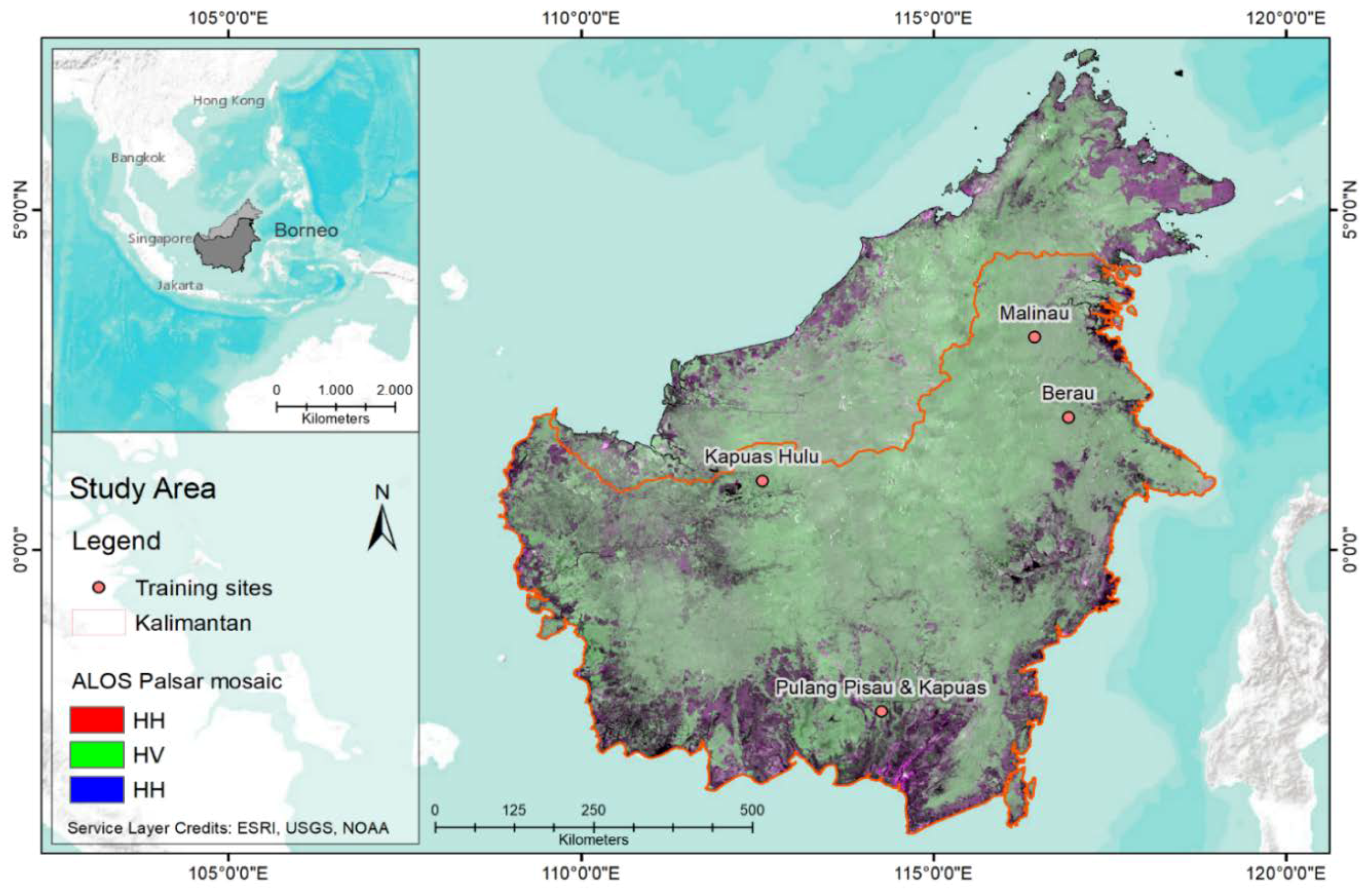
Kalimantan, which is the Indonesian part of Borneo island, has a size of about 544,000 km2 and lies within the geographic coordinates 4°15′41″N to 3°45′44″S latitude and 108°48′0″E to 118°49′41″E longitude (Figure 1). The island’s climate is mainly conditioned by the dry southeast monsoon from May to October and the wet northwest monsoon from November to April, and is influenced by frequent rainfall and high temperatures throughout the year. Those conditions are ideal for plant growth, which is why Kalimantan’s land cover is characterized mainly by tropical forests covering 301,750 km2 and, thus, more than 55% of the country. The forests of Borneo are considered to be one of the oldest and most species-rich tropical rainforests on Earth. The dominating forest ecosystems are mangrove forests, peat swamp and freshwater swamp forests, riparian forests, heath forests, lowland dipterocarp forests, ironwood forests, forests on limestone and ultrabasic soils, hill dipterocarp forests, and various montane formations [6]. In general lowland dipterocarp and peat swamp forests can be well discriminated in the field by means of average tree height, tree crown diameter, canopy closure, and species composition. Lowland dipterocarp forests are more diverse with taller trees and a more closed canopy [6]. Dipterocarps can reach a height of 45–60 m and are a valuable tree species prone to logging. All of the forest types store an extensive amount of carbon [8]. Nevertheless, the most significant carbon sinks in this area are belowground peatlands, which can store up to ten times more carbon than the forests growing on top them, since they were formed over the past millennia, as plant debris accumulated under waterlogged conditions [37]. The last decades witnessed a decrease of forest due to illegal logging, deforestation for agricultural development but also due to natural and manmade fires. Additionally, the ability of peatlands to store carbon is reduced due to anthropogenic activities like logging and drainage. In particular, draining the normally waterlogged peatlands makes these ecosystems vulnerable to fires. For modelling the reference AGB layer a universal AGB model is used for all different forest types.
2.1. Above-Ground Data
For the creation of the AGB reference layer existing field inventory data, collected across different forest types using the nested plots method, based on the guidelines provided by [38], were utilized. The methodology varies slightly for the various study sites, since they were processed as part of different research projects. The data was gathered in four test sites across Kalimantan (Figure 1) during 2007, 2009, and 2016 (Table 1). In order to estimate AGB using allometric models after [39], information about forest type, tree species, the diameter at breast height (DBH), and tree height are collected within nested plots based on three or four subplots. Inside the different subplots, trees of a certain diameter at breast height (DBH) were measured, for example, DBH < 10 cm (within the 3 m radius), ≥10 cm to <20 cm (10 m radius), ≥20 cm to <50 cm (20 m radius), and ≥50 cm (30 m radius). The sum of the measured parameters of the subplots was multiplied by an expansion factor in order to obtain the final values for 1 ha. In Pulang Pisau and Kapuas three circular subplots with radii of 20 m, 14 m, and 4 m, and 16 m, 8 m, and 4 m, and in Berau, Malinau and Kapuas Hulu four subplots with radii of 30/35 m, 20/25 m, 10 m, and 3 m were applied. In addition to circular nested plots, information was collected in rectangular plots of 20 m × 50 m to record saplings and trees in regrowing areas in Pulang Pisau and Kapuas. Moreover, nested rectangular plots with three subplots with sizes of 10 m × 10 m, 20 m × 20 m, and 20 m × 50 m were applied in Kapuas Hulu.
Airborne LiDAR measurements were acquired during the dry seasons in 2007, 2011, and 2012 in the same areas as the field data was collected. In 2007 (May–October) a Riegl LMS-Q560 2D laser scanner by RIEGL Laser Measurement Systems GmbH (Horn, Austria) was flown at a height of 500 m above-ground and a half scan angle of ±30° to collect the full-wave LiDAR data. The average point density of the final data 2007 was 1.5 points per m2. For the years 2011 and 2012 (August–October) the measurements were acquired using Optech Orion M200 and Optech ALTM 3100 airborne laser scanners by Teledyne Optech (Vaughan, Ontario, Canada) at an altitude of 800 m above-ground. A half scan angle of ±11° was used and the point density amounted to 10.7 points per m2. Since the accuracy of biomass estimations derived from LiDAR metrics increase with a higher point density, a weighting of the plots accordingly to their point density was applied [40]. In total, 8300 km2 were surveyed in different regions in East, West, and Central Kalimantan (Table 1) representing different ecosystems. Since there was a lack of LiDAR data for 2016 due to vast fires in Kalimantan, adjusted data of 2011 and 2012 was used.
2.2. Earth Observing Datasets
2.2.1. SAR Data
SAR data was acquired in 2007, 2009, and 2016, using years with preferably dry conditions and less active fires. The study is based on L-band radar data of the Phased Array Type L-band Synthetic Aperture Radar (PALSAR), onboard the Advanced Land Observing Satellite (ALOS) of the Japan Aerospace Exploration Agency (JAXA) and ALOS-2 in combination with C-band radar data based on ENVISAT ASAR and Sentinel-1. ALOS PALSAR and ALOS-2 PALSAR-2 mosaics with a spatial resolution of 25 m were provided by the Kyoto and Carbon Initiative. ENVISAT ASAR was launched in 2002 by the European Space Agency (ESA). Sentinel-1a and Sentinel-1b C-band radars were launched within the Copernicus program by the ESA in 2014 and 2016, respectively. ALOS PALSAR (HH, HV) images were used to estimate the biomass in Kalimantan for the years 2007 and 2009. As C-Band radar data for the years 2007 and 2009 imageries of ENVISAT ASAR (VV) data were tested, certainly the data had to be excluded as the study area is not fully covered by scenes acquired in one sensor mode and because of strong moisture effects. In 2016, data of ALOS-2, launched in 2014, in combination with Sentinel-1 GRD data, acquired in interferometric wide (IW) swath and a resolution of 10 m × 10 m, was used.
2.2.2. SRTM
The Digital Elevation Model (DEM) from the Shuttle Radar Topography mission (SRTM) with a vertical accuracy of ±10 m and a spatial resolution of 30 m is used for topographic analyses. Slope is used to clean up the final AGB map, since extreme overestimation of biomass occurs in steep terrain. Besides, steep terrain can cause layover and shadow effects, decreasing the accuracy of the AGB estimation.
2.2.3. TRMM
Since SAR backscatter is highly sensitive to water content of the surface due to its dielectric properties, daily TRMM (Tropical Rainfall Measuring Mission) of the National Aeronautics and Space Administration (NASA) and JAXA precipitation data with a spatial resolution of 0.25° were incorporated in order to select satellite acquisition dates with dry and comparable conditions [41].
2.2.4. MODIS Active Fire Data (MDC14DL)
MODIS hotspot information (product MCD14DL, provided by NASA) were used as an additional layer to detect thermal anomalies and active fires in Kalimantan. In this layer active fires are represented in the center of a 1 km × 1 km pixel that is identified by the MODIS MOD14/MYD14 Fire and Thermal Anomalies algorithm as containing one or more fires within the pixel [42,43].
2.2.5. Water Body Mask
ESRI World Water Bodies was used for delineating water bodies within the study area. It provides a base map layer for lakes, seas, oceans and large rivers and as generated on data with a spatial resolution of 100 m [44].
2.2.6. Urban Areas
The ESA CCI land cover map provides three epoch series (2000, 2005, 2010) of global land cover maps at 300 m spatial resolution which were used to evaluate settlement areas. ESA CCI land cover maps were produced used a multi-sensor and multi-temporal strategy based on MERIS Full and Reduced Resolution (FR and RR) archive. The 10-year product has been served as a baseline to derive the 2000, 2005 and 2010 maps using MERIS and SPOT-Vegetation time series specific to each epoch [45].
3. Methods
3.1. Above-Ground Biomass Data
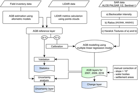
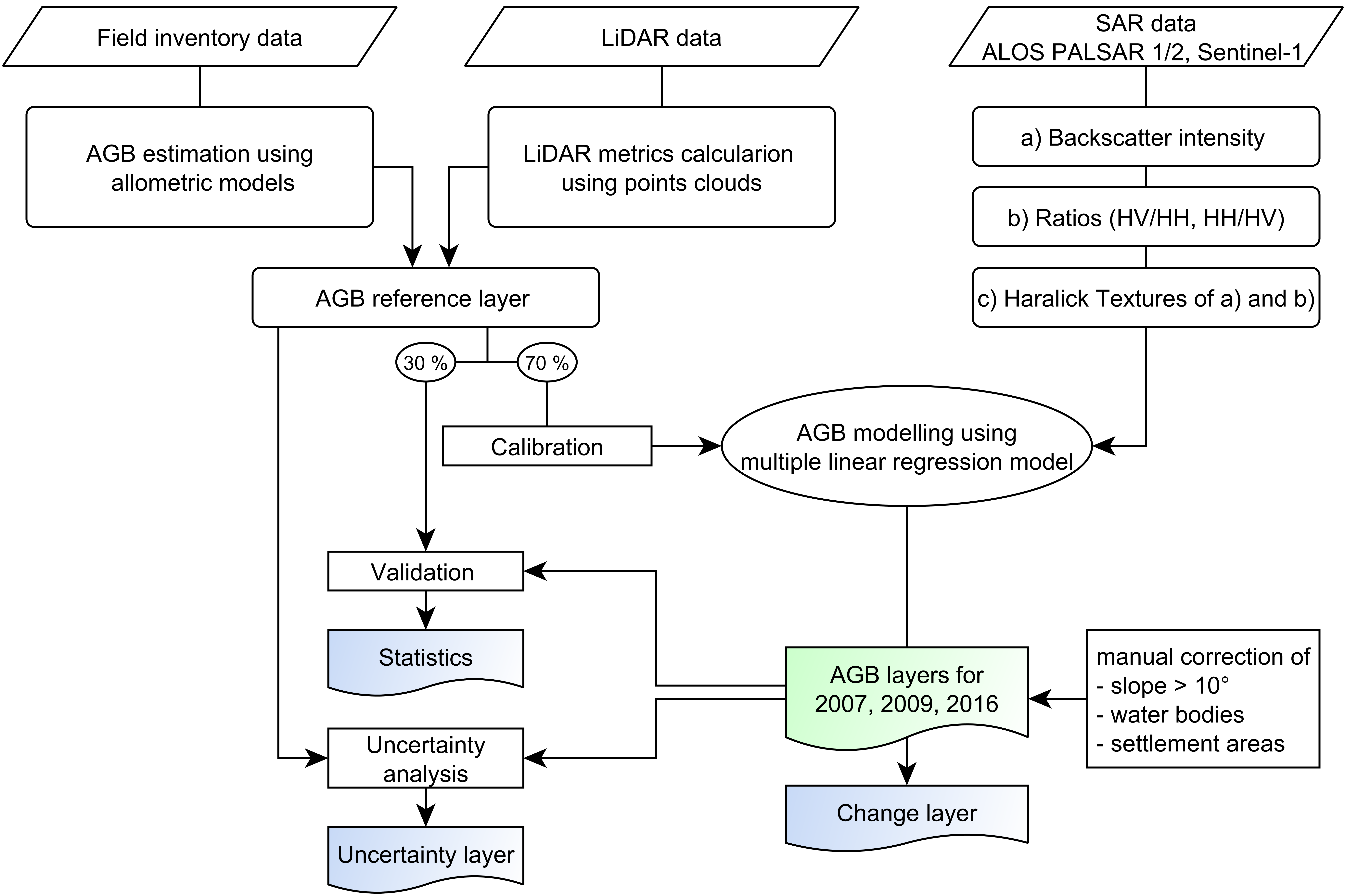
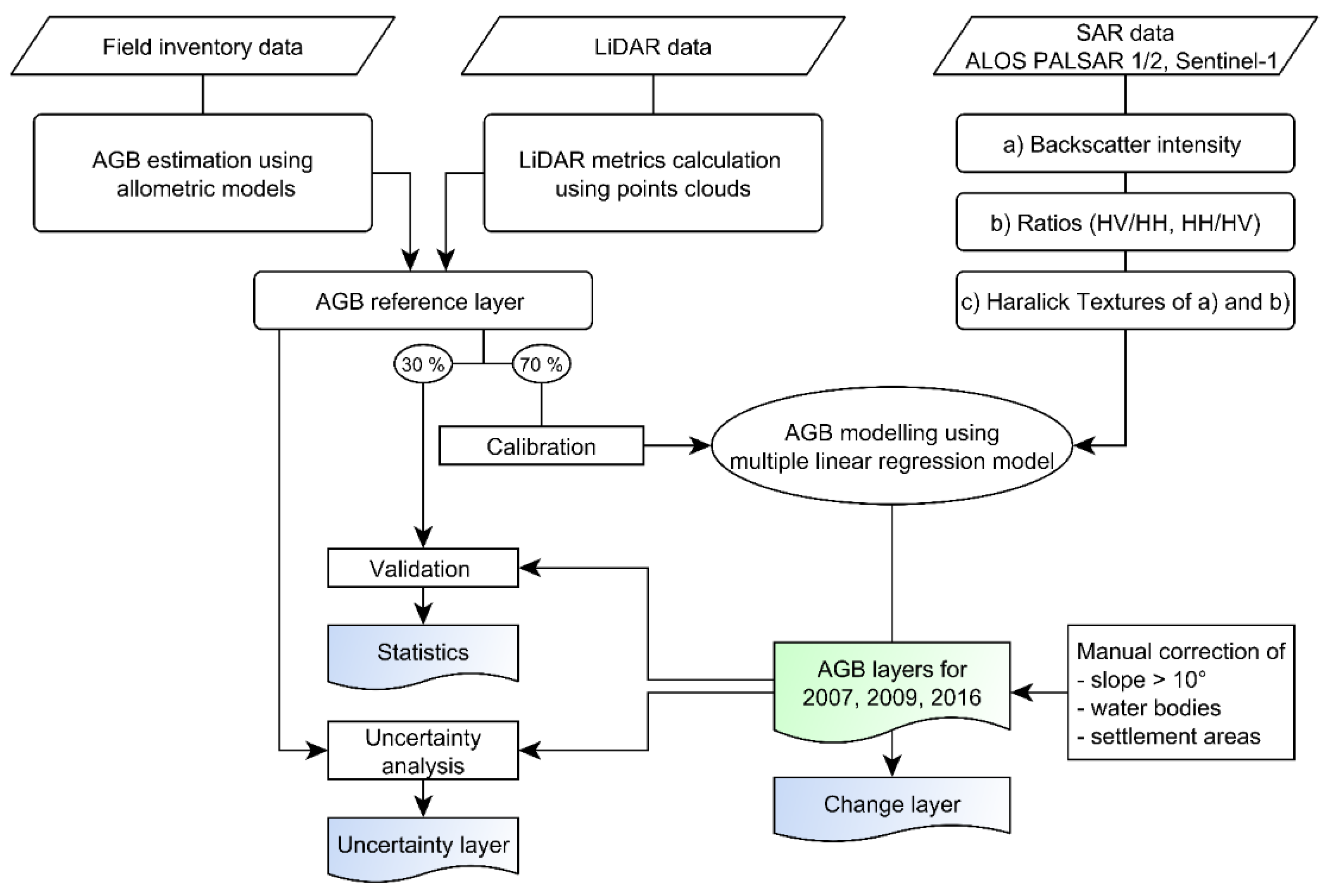
Inventory data and LiDAR data are combined to create more accurate biomass predictions for an area within the SAR images. This upscaling from field inventory to LiDAR transects allows creating a more precise basis for AGB model calibration and validation from SAR backscatter data [40]. An overview of the whole methodology of this study can be found in Figure 2.
The estimation of AGB in t/ha from field inventory data was achieved by using the tree height, diameter at breast height (DBH), and wood specific density of each tree as the input for a combination of different allometric models. Therefore, allometric models from [46] for saplings (if DBH < 5 cm and height ≤ 1.3 m) or trees (if DBH < 5 cm and height > 1.3 m) and from [39] for moist tropical forest stands (if DBH ≥ 5 cm and height > 1.3 m) were applied. Those ground-based AGB values were related to LiDAR transects in order to estimate biomass reference data using previously-established regression models for the different study sites, as described in [40].
LiDAR height histograms were calculated by normalizing all points within a grid of, e.g., 30 m (similar to the size of the largest nest of the field inventory plots) to the ground using a DTM as reference, i.e., the height of each LiDAR return was calculated relative to the DTM [47,48]. The number of points within each 0.5 m interval was stored as a histogram. The first (lowest) interval was considered as the ground return and excluded from further processing. The LiDAR data enabled calculating the two LiDAR point cloud metrics quadratic mean canopy height (QMCH) and centroid height (CH), as described more in detail in [40]. Previous studies have shown that those two parameters are able to estimate tropical forests AGB, as they take into account the point distribution of the LiDAR measurements [47,49]. This is why the QMCH and the CH were estimated based on height histograms by weighting each 0.5 m height interval by the fraction of points within the interval. CH and QMCH were related to AGB, estimated by the field inventories using regression models for each particular study site in order to obtain large-scale biomass estimations [29,48]. Furthermore, the point density was included in the regression model, since [47] showed that the accuracy of AGB estimations derived from LiDAR height histograms increased with higher point densities. The coefficient of determination (R2) of the AGB regression models vary from R2 = 0.7 (Berau and Kapuas Hulu) to R2 = 0.8 (Malinau and Central Kalimantan).
The upscaling from field inventory data to LiDAR transects allows creating numerous biomass reference data for the calibration of SAR images and to upscale AGB across large areas and different ecosystems. It provides AGB estimates over the whole biomass range from woody regrowth to pristine forest, and is able to disclose a spatial variation due to varying growth conditions. In order to estimate AGB based on SAR data the reference AGB was rescaled to a spatial resolution of 100 m.
Since there was a lack of LiDAR data for 2016 due to vast fires in Kalimantan, the data of 2011 and 2012 was used. Differences between the reference AGB and the SAR images over time were detected and excluded using MODIS fire hotspots, as fire is the main reason for deforestation in this area.
3.2. SAR Data
Since SAR backscatter is highly sensitive to water content of the surface due to its dielectric properties, daily TRMM (Tropical Rainfall Measuring Mission) precipitation data with a spatial resolution of 0.25° were used to verify the moisture conditions within the SAR imageries. In order to have dry and comparable conditions images with a high influence of precipitation were excluded. During the pre-processing of the Sentinel-1 (10 m) and ALOS PALSAR (25 m) data a co-registration based on an ALOS PALSAR mosaic with a spatial resolution of 25 m, a radiometric calibration estimating γ0 backscatter coefficients in dB and a geometric correction were accomplished. Furthermore, a multi-temporal speckle filtering using an enhanced Lee filter with a 7 × 7 window was applied [50]. The processed data was resampled to a resolution of 100 m resulting in pixels with a spatial resolution of 1 ha.
In order to examine the potential for AGB estimation, ratio images were prepared, using the following equations:
where HH, HV, VV, and VH indicate the polarization of the γ0 backscattering coefficients, depending on available polarizations of ALOS PALSAR and Sentinel-1. An evaluation of ratios and textures can be found in [51].
Rhvhh = HV/HH
Rvhvv = VH/VV
To improve the model accuracy, Haralick textures [52] and their relationship to AGB were also investigated. Texture describes the properties of objects, such as regularity, smoothness, and tonal variation [51]. Ten simple Haralick textures applying a gray level co-occurrence matrix (GLCM) and eleven higher-order Haralick textures applying a gray level run-length matrix (GLRM) were calculated within the open-source software Orfeo ToolBox by CNES (Centre National D’Études Spatiales) over a moving window with user-defined radius based on single polarized images and the calculated ratios. The radius used for single polarized images had a size of five, while a radius of three was used for calculating textures based on ratios. The relationship between these generated SAR variables and the LiDAR AGB was analyzed and showed an inversely proportional correlation. The variables were linearized in order to use the variables as an input for a multivariate linear regression model (MLR).
3.3. Multivariate Linear Regression Model (MLR)
In Englhart et al. [53] it was found that artificial neural network (ANN) and support vector regression (SVR) were suitable to predict AGB in tropical forests. Nevertheless, in terms of biomass variability and saturation in tropical forest ecosystems, multivariate linear regression models (MLR) are superior to ANN and SVR models [53]. Since very high biomass values are expected in the study area, MLR is used to model the above-ground biomass. Multiple regressions are often affected by overfitting and co-linearity among variables. In order to find a model with the greatest explanatory power, a backward stepwise multiple linear regression was performed to automate the selection of the best explanatory variables. The MLR was first set up with all linearized ratios and textures and run iteratively. To decrease the number of inputs, the p-value and the variable inflation factor (VIF) were investigated for each variable to identify their significance and co-linearity. Regarding literature, parameters with a p-value <0.05 and a VIF >5 were excluded from the model [26,51,54]. After eliminating redundant information, three variables were finally used for 2007 and 2009 and four variables for 2016. However, the extreme fire events in 2015 burned vast forest areas in Kalimantan. Resulting burned and carbonized trunks enhance double bounce effects in this region, which caused higher backscatter values and, thus, an overestimation of the biomass model. To minimize the overestimation in this areas, a second model was set up for 2016 simply based on two variables that were less sensitive to high backscatter. This model was applied only in burned areas, captured by a mask based on high backscatter values. In the remaining parts of the scene the first model, using four inputs, was used.
Settlements and areas with steep terrains cannot be captured correctly by the model. In order to reduce errors due to radar shadow and layover effects, regions with a terrain steeper than 10° were excluded from the biomass estimation using the Shuttle Radar Topography Mission (SRTM) DEM. Mountainous areas in Kalimantan are less influenced by human activity since they are difficult to access and due to a lack of transport routes, like canals. For this reason, the forests in mountainous terrain are mostly unaffected by degradation. Altogether 27.2% of the study area of Kalimantan are influenced by slopes steeper than 10° the main forest type in these regions is the hill- and sub-montane forest which was determined during field inventory campaigns, as well as through detailed forest classification mapping covering the LiDAR areas. The mean value of LiDAR AGB was calculated for the area with a terrain steeper than 10° and resulted in 350 t/ha. Additionally, urban areas and water bodies were excluded from the final results, using an ESRI World Water Body layer and the ESA CCI land cover map of each particular year (2005, 2010, 2015).
3.4. Temporal Change Estimation
The temporal change between 2007–2009, 2009–2016, and 2007–2016 was assessed using the RMSE in order to define a possible biomass range for each estimate at pixel level. The RMSE is calculated for five classes 0–50 t/ha, 50–100 t/ha, 100–150 t/ha, 150–200 t/ha, and >200 t/ha. The specific RMSE of the corresponding AGB range was subtracted from and added to the estimated AGB value at pixel level. The results are two layers consisting of the highest (H) and lowest value (L) of a possible AGB range per pixel for two comparing time-steps (T1, T2). A change/no-change mask, with discrimination of the increase and decrease, was generated by using threshold values based on the following decisions. If HT1 > LT2 or LT1 < HT2, an overlap between the ranges exist and, thus, no-change is assumed. In cases where HT1 < LT2, we suppose an increase of AGB and if LT1 > HT2 a decrease of AGB between the two years, both indicates a change. In order to remove single separated pixel, a minimum change unit of 300 m × 300 m was applied.
3.5. Validation and Uncertainty
For the validation of the AGB estimation, field inventory and LiDAR data, was used. The data was randomly split into data used for training (70%) and validation (30%) of the SAR-AGB models. For each map approximately 500 points were randomly set within the reference layer extent. To measure the accuracy of the models different parameters like bias, RMSE, standard deviation (SD) and the R2 were calculated for each map within an AGB range of 50 t/ha starting from 0 up to >200 t/ha and the overall range. Additionally, the NSE was estimated for the overall biomass range. Regarding [55], the NSE is a dimensionless index measuring the efficiency of a model in a range from −∞ to 1. The closer the NSE is to 1, the more accurate is the model. The NSE is calculated using the following equation:
where N is the number of observations, Pi is the predicted value, Oi is the observed value, and is the mean of the observed value [55].
An uncertainty map at the pixel level is important for the interpretation of AGB maps, as shown in [56,57]. The total uncertainty at the pixel level is composed of different sources of errors which are assumed to be random and independent. These are propagated for each map using the equation proposed by [30], taking into account the errors of measurement, allometry, sampling size, and prediction. Similar to [26], a measurement error supposed to be 10%. In [39] the authors found an error for the estimation of a tree’s biomass of approximately ±5%. As we mainly used this allometry, an error of 5% is assumed. According to [30,58], a sampling size error of 20% is supposed. The prediction error includes the sampling error associated with the representativeness of the training data of the actual spatial distribution of AGB and the model predictions and is estimated per pixel.
4. Results
4.1. Modelling Results
Using a backward stepwise approach allows to reduce the parameters within in the MLR, resulting in the finally-used variables listed in Table 2. In addition, coefficient of determination and residual standard error are displayed for each model calibration. Model 1 and model 2 of 2016 are used in combination, whereas model 2 is only applied in burned areas. The overall R2 of the combined models is 0.69. The RP and the Low Grey-Level Run Emphasis (LGRE) showed the best relationship to LiDAR AGB compared to all Haralick textures. Additionally, cross-polarized-based parameters perform significantly better than co-polarized ones.
4.2. Biomass Maps and Temporal Change
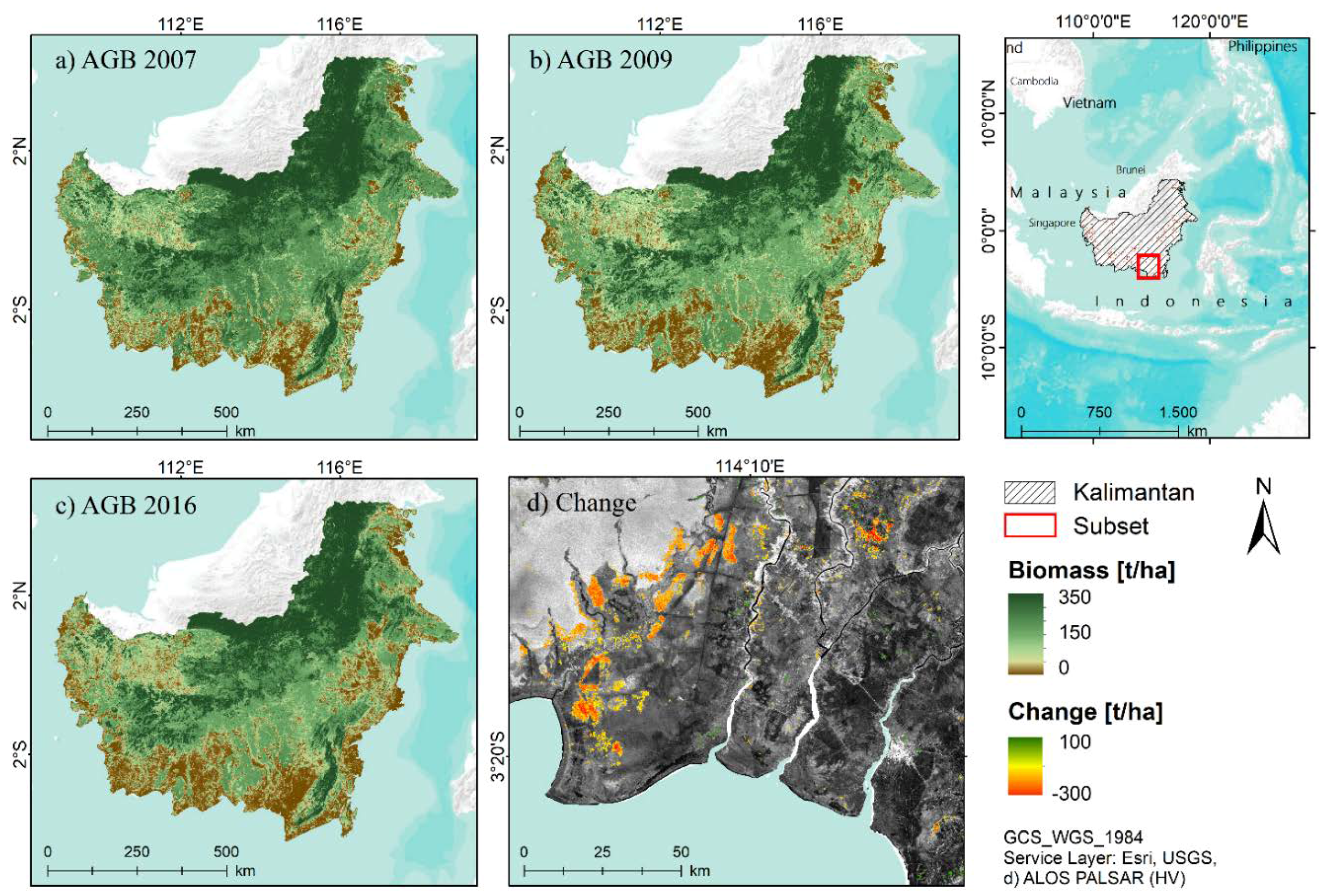
The final biomass maps with a resolution of 100 m are presented in Figure 3a–c. Kalimantan is dominated in all years by forests with biomass varying in a range of 50–350 t/ha. However, its land cover is changing in time. Areas close to the coasts and along rivers show low biomass values between 0–50 t/ha. In 2007 15% of Kalimantan was covered by non-forested areas. Certainly, the portion of this class is growing over the years, caused by a decrease of forest and, thus, a loss of biomass. In 2009 the amount of non-forested extents is about 20%, though it reaches the maximum (25%) in 2016. The highest biomass values are reached in areas of mountainous terrain, which can be found in the north and center of Kalimantan. Nevertheless, the extent of forests containing high biomass values is significantly shrinking. In 2007 the model found a percentage of 55% of Kalimantan with biomass values >200 t/ha, while it is 38% in 2016. The biomass variability due to different degradation stages in the forest, as well as different disturbances in contrast to non-disturbed areas or clear-cuts, can be captured in the final maps.
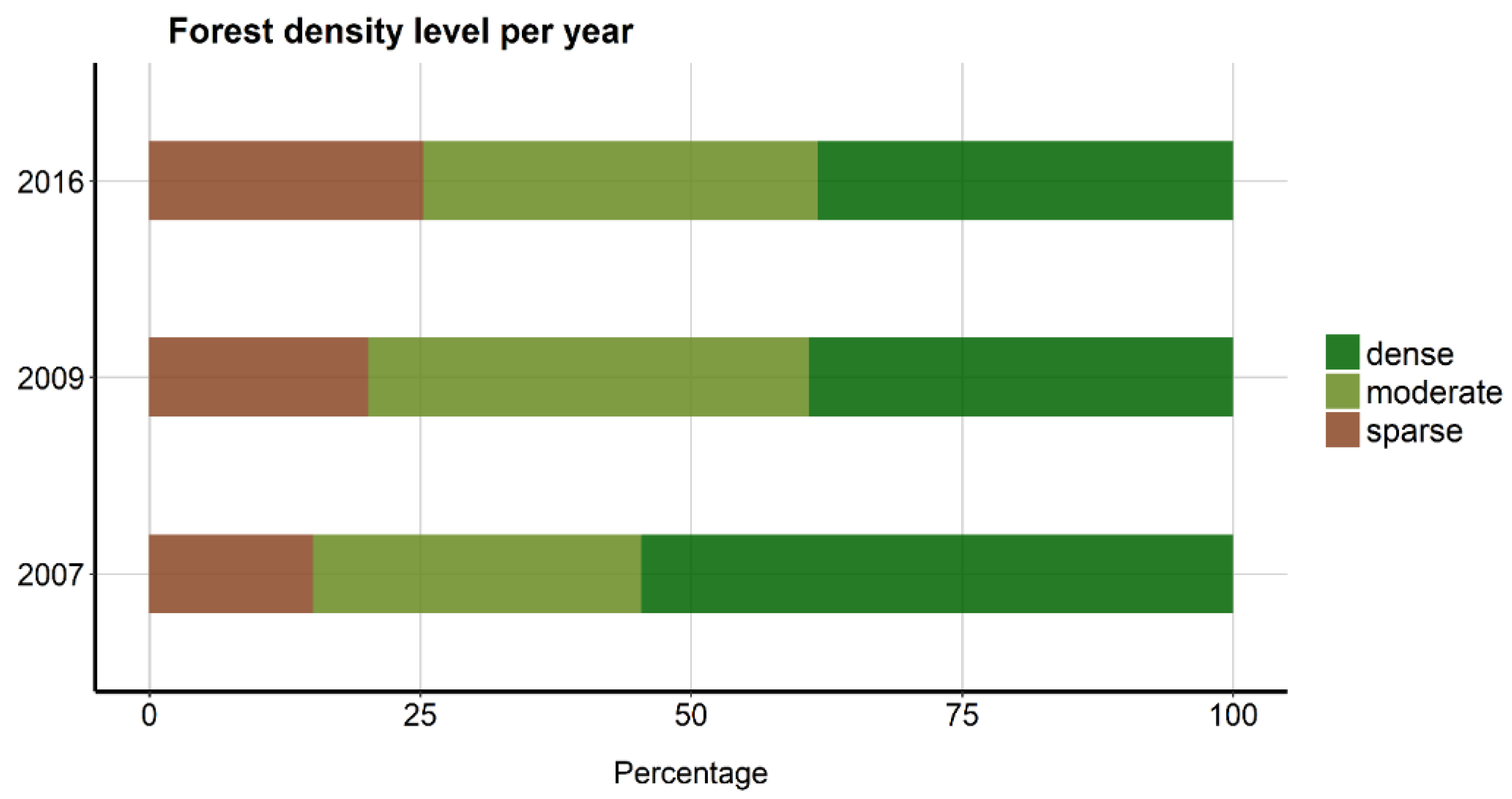
A subset of Kalimantan, showing the change in the south of the island for the period 2009–2016, is displayed in Figure 3d. Red colors show a decrease of biomass, while green colors indicate an increase of AGB. The region is mainly dominated by a loss of biomass with values about − 300 to −100 t/ha. In contrast, only few areas show increased biomass. A similar distribution can be observed across the entire coastline of Kalimantan. Mountainous regions in the center of Kalimantan are less influenced by change. Figure 4 is summarizing the percentage of the forest degradation level per year. Highly-degraded areas increase from 15% in 2007 to 20% in 2009 to 25% in 2016. Accordingly, the area covered by natural forest (AGB > 200 t/ha) decreases. The coverage of forested areas containing an AGB from 50 to 200 t/ha are rising since areas with natural forest are affected by illegal logging, where single trees are felled. Thus the class of natural forest is slowly converted into degraded forest. Ongoing activities are further converting the degraded forest to highly-degraded areas.
4.3. Comparison with Pan-Tropical Biomass Maps
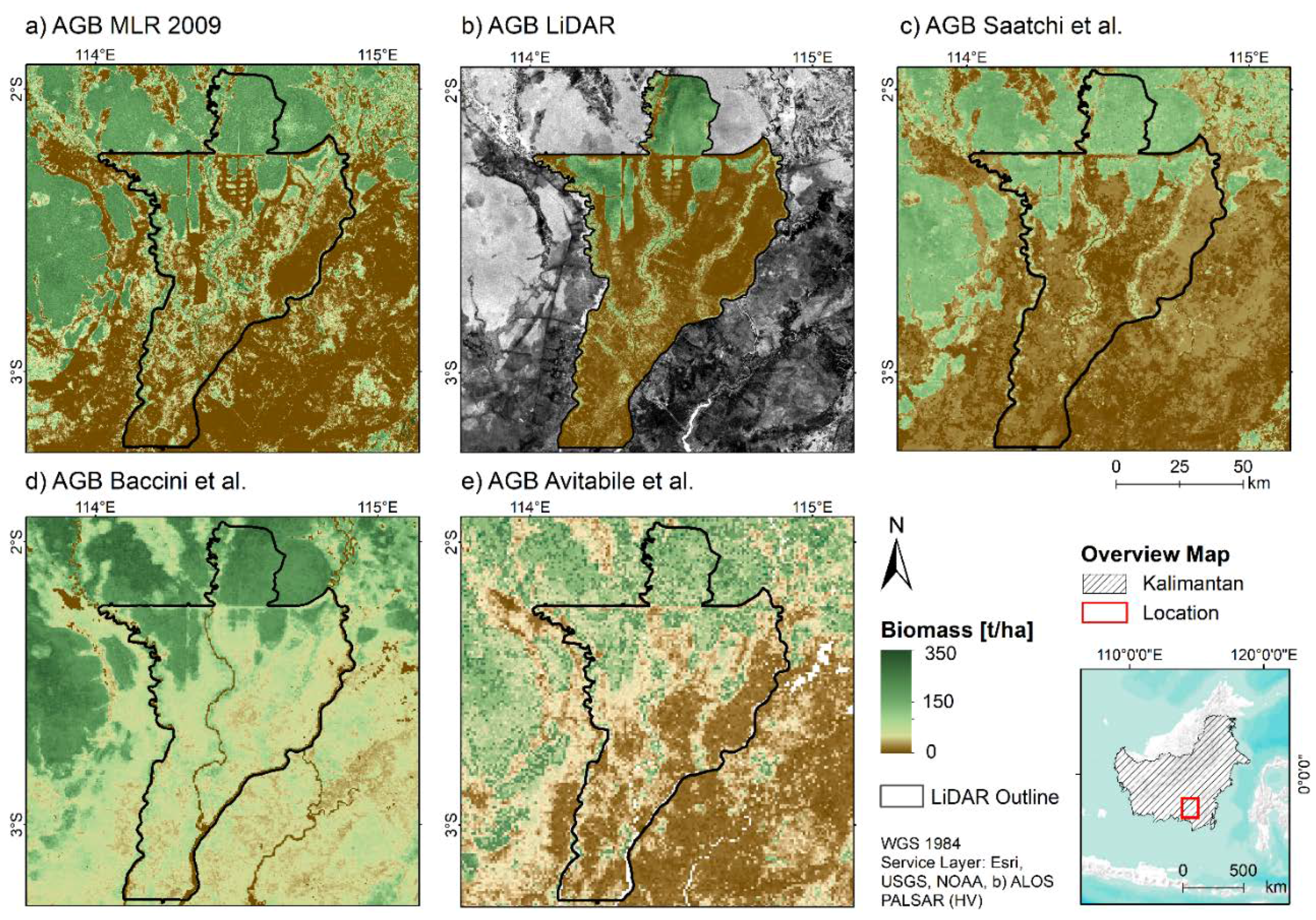
Figure 5 displays a subset of a degraded peat swamp forest in Central Kalimantan near the capital Palangka Raya. A visual comparison of the estimated AGB map, the LiDAR-derived reference AGB map and other pan-tropical biomass maps [7,30,36] with a resolution of 500 m and 1 km, respectively, points out that the developed MLR model correctly estimates the variability of biomass. The biomass map of [7] overestimates AGB in the lower biomass ranges and is not identifying heterogeneity in forests in detail. In contrast, the map of [30] underestimates high biomass ranges, but captures disturbances in forested areas. Avitabile et al. [36] combine the pantropical biomass maps of [7] and [30] and additional data in order to create an improved pan-tropical biomass map. The final product of [36] with a resolution of 1 km has a lower RMSE and bias than the two previous studies. Comparing maps (a) and (e), a similar trend of the biomass distribution is visible. The estimated AGB map based on the MLR model has a much finer resolution (100 m) which allows visualizing AGB variability more precisely and detects even small-scaled changes for carbon modelling, as well as forest monitoring or risk managing systems. Moreover, the modelled maps show a better accordance to the LiDAR-derived AGB in the subset.
4.4. Validation and Uncertainty
Various validation statistics of the estimated AGB in Kalimantan, calculated using approximately 500 points per map, are listed in Table 3. The sample points were randomly distributed over areas, where reference data was available (training sites, Figure 1). Average AGB estimates are consistently higher than those obtained from the reference biomass, except to the AGB range >200 t/ha. Higher averages indicate a positive bias, while the magnitude of the bias is variable across the AGB ranges and points to the highest values in the biomass classes of 50–100 t/ha and 100–150 t/ha. In contrast, AGB ranges >200 t/ha display a negative bias. The root mean square error (RMSE) is similar in all years, with the highest relative errors exceeding 100% in the lower AGB ranges and low relative errors of around 22% in the highest AGB ranges. The distribution of the relative RMSE is similar in all three years. The relative overall RMSE ranges between 31% (2016), 36% (2009), and 38% (2007). The scatterplots of AGB estimates against the reference AGB display a similar distribution in all years (Figure 6). AGB values up to 250 t/ha show an overestimation of the models, especially in 2007, while AGB ranges higher than 250 t/ha indicate an underestimation. The coefficient of determination (R2) varies in a range of 0.69 in 2016 to 0.77 in 2007 and the standard deviation (SD) is 53 t/ha in 2009 and 2016 to 56 t/ha in 2007. The NSE, indicating the efficiency of a model in a range from −∞ to 1, shows a good model performance for all years, reaching values between 0.70 and 0.76.
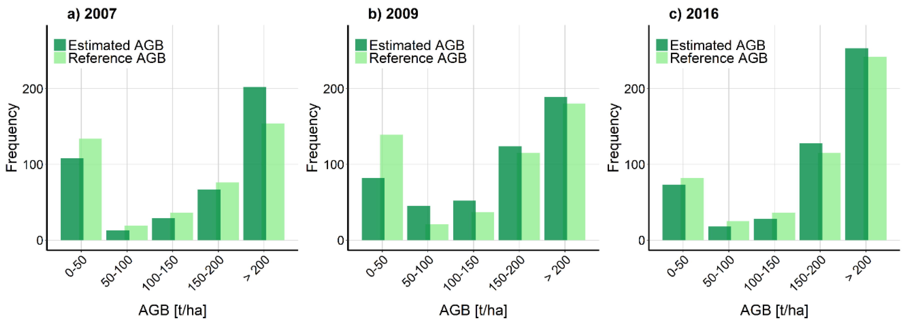
Figure 7 shows the number of sample points (frequency) of the reference AGB in contrast to the estimated AGB in each biomass range. The distribution of the frequency for the reference and the modelled biomass per range are similar, showing just small discrepancies in each year. The histogram of 2007 is affected by a smaller frequency of estimated biomass in each range, except the range >200 t/ha with a relative error of about 25%. In contrast, the histogram of 2009 is dominated by a lower sum of observations per range for all ranges except the smallest biomass range (0–50 t/ha) with a relative error of 42%. 2016 shows only little differences in each biomass range.
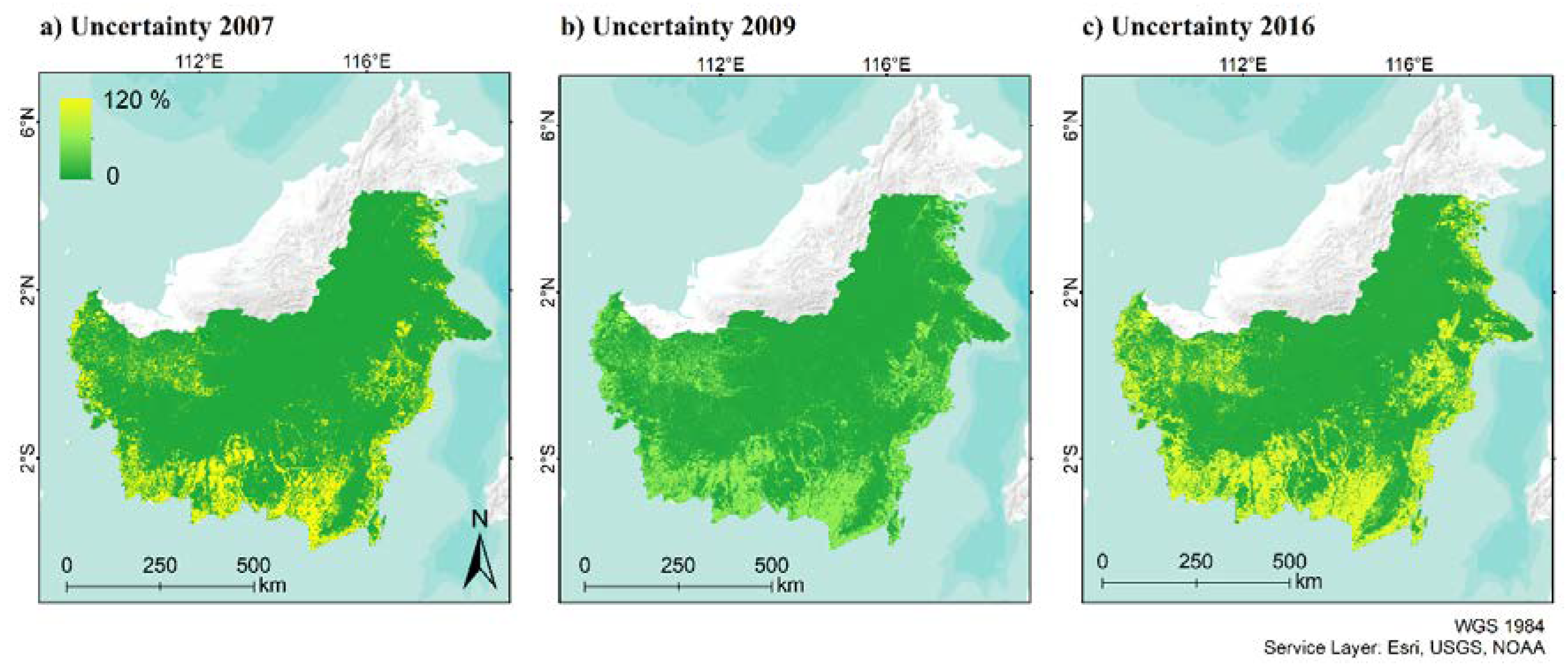
The uncertainty per AGB range (Figure 8), computed as a percentage of the AGB estimates, shows the highest relative errors in areas with low AGB estimates (Table 4). The relative errors in the biomass range 0–50 t/ha vary between 61.3% to 117.9%, in which the lowest values were obtained in 2009 and the highest in 2007. Areas with high biomass estimates show low relative errors of about 6% in each year. Additionally, the overall relative error per year show similar values varying in a range from 7.8% to 9.1%.
5. Discussion
5.1. Biomass Estimation
The results suggest that a MLR using backscatter values in combination with ratios and textures of ALOS PALSAR-1/2 L-band and Sentinel-1 C-band data is eligible to model AGB in tropical forests. Englhart et al. [53], the authors found that in terms of biomass variability and saturation in tropical forest ecosystems MLR models are superior to ANN and SVR models. Since Kalimantan is dominated by high biomass values, a MLR was, therefore, used to model the AGB.
The use of highly accurate field inventory plots in combination with extensive LiDAR surveys as reference datasets improved the SAR-based biomass modelling. These datasets were collected in different ecosystems across Kalimantan, covering a wide range of ecosystems, vegetation types, forest structures and, thus, biomass ranges, for which reason they provide more precise biomass estimates than other sensors or the exclusive use of field inventory data [40]. Nevertheless, uncertainties between field data and the modelled reference AGB can originate from different factors. First of all, the lag time between field data and LiDAR data acquisitions can introduce uncertainties due to regrowing or deforestation. For the reason that LiDAR data was not available for 2016, LiDAR data from 2011/2012 was adjusted as the reference layer for 2016. In order to minimize the effect of this temporal shift additional MODIS hotspot data (MCD14DL) was used to eliminate burned areas between 2011 and 2016. Certainly, forest cover changes resulting from logging or regrowing is not captured and can cause inaccuracies. Second, extrapolating field inventory data can introduce errors, since the spatial variability cannot be covered. In addition, the accuracy and precision of AGB extrapolated from field plots are affected by plot size and shape [59]. Previous studies showed that errors in LiDAR-estimated AGB decrease exponentially with increasing field plot size, resulting from a smaller effect of co-registration errors and a spatial averaging of errors [58,59,60,61]. In contrast, smaller plots have less overlap with the LiDAR data, cannot capture the variability of a forest, and are more sensitive to individual trees [13,62]. For lack of data, differing field plot sizes and shapes were used to estimate the reference AGB. However, most of the used field plots exceed an area of 1000 m2, which is sufficiently large to be more robust against boundary effects [59,63,64]. In contrast, Mauya et al. [65] show improvements of the model accuracy with increasing plot sizes in a range from 200–3000 m2. In addition to the size, the shape affects the precision and accuracy of the extrapolated biomass. Circular plots are less influenced by the circumference to area ratio than rectangular ones [65]. As the number of rectangular plots in this study is limited and only within regrowing forest areas, their influence in AGB estimation is marginal. The uncertainty resulting from different sampling strategies are considered as the error of sampling size in the overall uncertainty of the SAR model with 20% [58]. Finally, uncertainties may also be introduced by reason that a universal AGB model was applied for different forest types [66]. Since tropical forests consist of hundreds of different tree species species-specific regression models cannot be applied [39].
After creating a reference biomass layer from LiDAR and field inventory data, AGB can be estimated for large-scaled areas using remote sensing data. The applied SAR backscatter approach is well known for radar-based forest cover and biomass mapping. It is computationally less intensive than alternative approaches and transferable to other regions, but also limited by some factors like backscatter saturation and backscatter variations due to terrain and wetness [19,67]. The resulting maps point that the biomass variability due to different degradation stages in the forest, as well as disturbances in contrast to non-disturbed areas or clear-cuts that can be captured very well. The R2 varies in a range of 0.69 in 2016 to 0.77 in 2007 and the NSE shows good model performance for all years, reaching values between 0.70 and 0.76. Studies modelling biomass and carbon based on ALOS PALSAR HV backscatter values in tropical forests found similar correlations, varying from 0.407 to 0.76 [68,69,70]. Nevertheless, all maps show an underestimation at higher AGB levels compared to reference AGB. In addition to the underestimation in higher biomass ranges, biomass in lower AGB ranges is overestimated. Similar distributions of estimated biomass are shown in other regional studies estimating biomass from SAR backscatter values for different forest ecosystems, as a characteristic of SAR data for high biomass levels [17,66,71,72].
One of the general limitations of the applied approach is that SAR-based AGB retrieval suffers from saturation of the backscatter signal in the higher biomass range. The saturation level varies amongst others with the sensor wavelength and polarization, as well as the forest structure [20]. AGB studies in tropical forests, such as in Kalimantan, were mostly conducted on the basis of L-band SAR data, being the most suitable operational data for biomass estimation [24,25,26,27,28]. The saturation level in tropical forests, using the L-band, varies around 50 t/ha to 200 t/ha [25,30,72]. Comparable to Thapa et al. [51], the present study uses backscatter values and, additionally, backscatter ratios and textures, which increases the saturation level to approximately 200–250 t/ha. A higher amount of ratios and textures based on backscatter values of different polarizations could further improve the model results, as shown in [51]. With an increasing model complexity, the correlation and the NSE also increase in a range from 0.62 to 0.84 and from 0.54 to 0.83, respectively.
Another limiting factor of the backscatter approach are the moisture conditions of soil and vegetation [73]. Especially in tropical forests, located in areas with a high amount of annual precipitation, the estimation of biomass based on backscatter can causes errors. To reduce humidity effects, scenes acquired during different periods of the year were averaged. Furthermore, images with a high influence of precipitation were excluded from the mosaics by incorporating TRMM data as selection criteria. Analogous to literature, variables based on HV backscatter were found as less influenced by changes in moisture and topography conditions at longer wavelengths and more sensitive to biomass than co-polarized data [21,25,30,34,70,72]. However, even with the use of variables based on HV polarization, moisture effects can cause differences in the biomass estimation for the different years [74]. The very dry conditions in 2007 may be an explanation for the higher backscatter saturation in 2007 and, thus, a better overall correlation. The lower R2 of 2016 may not only result from the higher amount of precipitation in 2016, but also from the distribution of the validation samples. In contrast to the other years, the biomass range >200 t/ha contains 45% of all samples, which makes this class the most influential. The distinct underestimation of this AGB range is reflected in the overall R2 of 2016. The given distribution of sample points originated because of the fire catastrophe in 2015, where a lot of areas within the reference biomass layer were burned. In order to reduce errors in the later modelling, those areas were excluded from the reference layer with the use of a MODIS hotspot product. The fires primarily occurred in areas that were already stressed by former burning or logging activities, accordingly in the lower biomass ranges, which leads to a lack of validation data in this class.
Furthermore, topography influences biomass estimation based on SAR data. To reduce possible errors caused by the effect of slope on radar backscatter, Mitchard et al. [26] suggested the use of a DEM, which is why we excluded AGB estimations in steep terrain with slopes >10°, an area of 27% of the study area. Since the mountainous areas are barely affected by degradation and human activity, those regions were manually set to a biomass level of a healthy natural forest, 350 t/ha, as derived from LiDAR data. Additionally, settlement areas are not reliable in the final AGB maps. The high backscatter values due to double bounce effects result in backscatter values similar to those of forests. The use of an additional urban layer allows to flag settlements in a quality assurance layer, which we provided for each map.
Since models are minimizing the bias and overall error in order to get the best fit, the overestimation in lower biomass ranges results from the model adjustment due to the inability of estimating higher biomass ranges correctly [75].
In contrast to [33,76] a combination of C- and L-bands in the model of 2016 shows only minor improvement in comparison to a single-band approach. The C-band is more sensitive to variabilities in surface roughness resulting in improved modelling in burned areas or grass cover, so the combination of the C-band with the L-band slightly improves the correlation of estimated and predicted biomass compared to the use of the L-band alone.
The final biomass maps have a spatial resolution of 100 m, which is much finer than other existing large-scale biomass maps from Indonesia by [30], yet with a comparable accuracy. Additionally, the model is transferable to other countries and regions, if precise reference data is available. The results have important implications for carbon-related projects, such as UN-REDD, and can help to achieve the objectives through supporting monitoring or risk managing systems. The fine-scaled resolution and the sensitivity to AGB variability of our products allow capturing even small-scale logging activities, and the results can be used as an early warning for more extensive changes of forests due to logging and fire vulnerability. Furthermore, the more accurate biomass maps can lead to more precise carbon estimations when used as input data for carbon-related models.
The results of the biomass estimation in tropical forests could be further improved using biomass estimation approaches based on coherence or phase instead of backscatter, but these methods are limited by data availability. A combined data approach using optical data/vegetation indices and SAR data could also enhance biomass estimation. The launch of new P-band satellites, like ESA’s Earth Explorer Biomass in 2021, will allow a more accurate estimation of biomass in tropical forests.
5.2. Temporal Change Estimation
To perform a change analysis a comparability of the three biomass maps is required. This is best accomplished using the same processing steps, model, reference, and radar data type for each map in order to avoid differences resulting from the methods and data. The three biomass maps of this study were generated using the same processing steps and model, but included Sentinel-1 as an additional sensor in the calculations for 2016. Differences between the three maps could also occur since different reference layers for each year were used. Nevertheless, the use of contemporaneous reference layers is essential, because of rapid changes in the landscape (e.g., fires and logging) and allows a more accurate calibration of the model. The use of two MLR models in 2016 may also cause discrepancies, since two variables were excluded from the second model. Using a confidence interval of 95% to identify changes allows a reduction of errors during the change mapping.
The resulting change maps show a significant loss of forest and, thus, biomass during 2007–2009, 2009–2016, and for the overall period 2007–2016. In addition to fires, changes can result due to illegal logging activities. The maps provide a helpful tool for REDD+, as well as national projects, since small-scaled deforestation is detected in an accurate and low-cost way for the entirety of Kalimantan over a period of approximately ten years using three time steps for the first time.
6. Conclusions
It was shown that a multivariate linear regression model using C- and L-band SAR-derived ratios and textures is able to model biomass more precisely and at a better resolution than existing models in this region. Nevertheless, the applied backscatter approach is limited by the fact that SAR-based AGB estimation is defined by saturation effects of the backscatter signal in higher biomass ranges. Due to the use of textures and the large amount of reference data, the saturation level could be increased to approximately 250 t/ha. Accordingly, the estimated AGB maps show an underestimation in higher AGB ranges, but also an overestimation in lower biomass ranges. The correlation of field biomass and estimated biomass varies in a span between 0.69 and 0.77. The model is able to capture biomass variability due to different degradation stages in forested areas. Additionally, different disturbances in contrast to non-disturbed area or clear-cuts can be identified. A biomass overestimation in urban areas and a reduced accuracy because of relief effects (layover, radar shadow) in steep slopes are known issues using SAR data and have been corrected via additional data. Sentinel-1 data, which was additionally used in 2016, did slightly improve the results. Modelling AGB for three different time steps allowed the estimation of change products. The change maps detected, for the first time, deforestation in an accurate and low-cost way for the entirety of Kalimantan over a period of approximately ten years based on three different time steps. The much higher spatial resolution of all products (100 m) allows capturing even small-scaled variabilities in forested areas, with the layer providing important assistance for recent UN-REDD projects and can help to achieve the objectives, as well as support monitoring and risk managing systems. Furthermore, the fine-scaled biomass maps can be used to estimate carbon stocks and carbon emission due to fires. The AGB estimation approach is transferable and allows modeling of biomass in other tropical forests with similar conditions in an accurate and less computationally intensive manner.
Author Contributions
S.L. and M.S. conceived and designed the experiments; A.B. and M.S. performed the experiments; A.B. and S.L. analyzed the data; F.S. supervised the project and commented on the manuscript; A.B., S.L. and F.S. discussed the results. A.B. wrote the paper.
Acknowledgments
The authors would like to thank the Japan Aerospace Agency for supplying ALOS PALSAR mosaics within the Kyoto and Carbon Initiative and the European Space Agency for providing Sentinel-1 data and for funding the study within the Globbiomass project (ESA contract no. 4000113100). We gratefully acknowledge Suwido Limin and his team from the Centre for International Co-operation in Management of Tropical Peatland (CIMTROP) as well as Hendrik Segah and his team from the University of Palangka Raya for the logistical support during the field surveys. The LiDAR dataset of 2007 was acquired by Kalteng Consultants. We would like to thank the Kalimantan Forests and Climate Partnership (KFCP) and AusAID (Australian Agency for International Development) for providing the 2011 LiDAR data. The Forests and Climate Change Programme (Forclime) lead by GIZ (Deutsche Gesellschaft für Internationale Zusammenarbeit) is highly acknowledged for providing field inventory and LiDAR data.
Conflicts of Interest
The authors declare no conflict of interest. The founding sponsors had no role in the design of the study; in the collection, analyses, or interpretation of data; in the writing of the manuscript; or in the decision to publish the results.
References
- World Bank Group. Forest Area (% of Land Area): Indonesia. Available online: https://data.worldbank.org/indicator/AG.LND.FRST.ZS?end=2015&locations=IDtart=2015&type=shaded&view=map&year=2010 (accessed on 2 February 2018).
- Page, S.E.; Hoscilo, A.; Langner, A.; Tansey, K.; Siegert, F.; Limin, S.; Rieley, J.O. Tropical peatland fires in Southeast Asia. In Tropical Fire Ecology; Springer Praxis Books: Berlin/Heidelberg, Germany, 2009. [Google Scholar]
- Tyrrell, M.L.; Ashton, M.S.; Spalding, D.; Gentry, B. Forests and Carbon: A Synthesis of Science, Management, and Policy for Carbon Sequestration in Forests; Yale School Forestry & Environmental Studies: New Heaven, CT, USA, 2009; Available online: http://environment.yale.edu/publication-series/5947.html (accessed on 7 March 2018).
- Van der Werf, G.R.; Morton, D.C.; DeFries, R.S.; Olivier, J.G.J.; Kasibhatla, P.S.; Jackson, R.B.; Collatz, G.J.; Randerson, J.T. CO2 emissions from forest loss. Nat. Geosci. 2009, 2, 737–738. [Google Scholar] [CrossRef]
- IPCC 2014. Climate Change 2014. Synthesis Report; Contribution of Working Groups I, II and III to the Fifth Assessment Report of the Intergovernmental Panel on Climate Change; Core Writing Team, Pachauri, R.K., Meyer, L.A., Eds.; Intergovernmental Panel on Climate Change: Geneva, Switzerland, 2015. [Google Scholar]
- MacKinnon, K.; Hatta, G.; Halim, H.; Mangalik, A. The Ecology of Kalimantan: Indonesian Borneo; Tuttle Publishing: New York, NY, USA, 2013. [Google Scholar]
- Baccini, A.; Goetz, S.J.; Walker, W.S.; Laporte, N.T.; Sun, M.; Sulla-Menashe, D.; Hackler, J.; Beck, P.S.A.; Dubayah, R.; Friedl, M.A.; et al. Estimated carbon dioxide emissions from tropical deforestation improved by carbon-density maps. Nat. Clim. Chang. 2012, 2, 182–185. [Google Scholar] [CrossRef]
- Page, S.E.; Rieley, J.O.; Banks, C.J. Global and regional importance of the tropical peatland carbon pool. Glob. Chang. Biol. 2011, 17, 798–818. [Google Scholar] [CrossRef]
- Jaenicke, J.; Rieley, J.O.; Mott, C.; Kimman, P.; Siegert, F. Determination of the amount of carbon stored in Indonesian peatlands. Geoderma 2008, 147, 151–158. [Google Scholar] [CrossRef]
- Olivier, J.G.J.; Janssens-Maenhout, G.; Muntean, M.; Peters, J.A.H.W. Trends in Global CO2 Emissions: 2016 Report; PBL Netherlands Environmental Assessment Agency: Den Haag, The Netherlands, 2015. [Google Scholar]
- Edwards, D.P.; Koh, L.P.; Laurance, W.F. Indonesia’s REDD+ pact: Saving imperilled forests or business as usual? Biol. Conserv. 2012, 151, 41–44. [Google Scholar] [CrossRef]
- Global Canopy Foundation. The REDD Desk. Available online: https://theredddesk.org/countries/search-countries-database?f%5B0%5D=type%3Aactivity&f%5B1%5D=field_project%3A1 (accessed on 7 February 2018).
- Goetz, S.; Dubayah, R. Advances in remote sensing technology and implications for measuring and monitoring forest carbon stocks and change. Carbon Manag. 2011, 2, 231–244. [Google Scholar] [CrossRef]
- FAO. Assessment of the Status of the Development of the Standards for the Terrestrial Essential Climate Variables; Biomass (T12); FAO: Rome, Italy, 2009. [Google Scholar]
- Bojinski, S.; Verstraete, M.; Peterson, T.C.; Richter, C.; Simmons, A.; Zemp, M. The Concept of Essential Climate Variables in Support of Climate Research, Applications, and Policy. Bull. Am. Meteorol. Soc. 2014, 95, 1431–1443. [Google Scholar] [CrossRef]
- Searle, E.B.; Chen, H.Y.H. Tree size thresholds produce biased estimates of forest biomass dynamics. For. Ecol. Manag. 2017, 400, 468–474. [Google Scholar] [CrossRef]
- Joshi, N.; Mitchard, E.T.A.; Schumacher, J.; Johannsen, V.K.; Saatchi, S.; Fensholt, R. L-Band SAR Backscatter Related to Forest Cover, Height and Aboveground Biomass at Multiple Spatial Scales across Denmark. Remote Sens. 2015, 7, 4442–4472. [Google Scholar] [CrossRef]
- Olesk, A.; Praks, J.; Antropov, O.; Zalite, K.; Arumäe, T.; Voormansik, K. Interferometric SAR Coherence Models for Characterization of Hemiboreal Forests Using TanDEM-X Data. Remote Sens. 2016, 8, 700. [Google Scholar] [CrossRef]
- Koch, B. Status and future of laser scanning, synthetic aperture radar and hyperspectral remote sensing data for forest biomass assessment. ISPRS J. Photogramm. Remote Sens. 2010, 65, 581–590. [Google Scholar] [CrossRef]
- Joshi, N.; Mitchard, E.T.A.; Brolly, M.; Schumacher, J.; Fernández-Landa, A.; Johannsen, V.K.; Marchamalo, M.; Fensholt, R. Understanding ‘saturation’ of radar signals over forests. Nat. Sci. Rep. 2017, 7, 3505. [Google Scholar] [CrossRef] [PubMed]
- Ghasemi, N.; Reza Sahebi, M.; Mohammadzadeh, A. A review on biomass estimation methods using synthetic aperture radar data. Int. J. Geomat. Geosci. 2011, 1, 776–788. [Google Scholar]
- Mermoz, S.; Le Toan, T.; Villard, L.; Réjou-Méchain, M.; Seifert-Granzin, J. Biomass assessment in the Cameroon savanna using ALOS PALSAR data. Remote Sens. Environ. 2014, 155, 109–119. [Google Scholar] [CrossRef]
- Hamdan, O. Assessment of Alos Palsar L-Band SAR for Estimation of above Ground Biomass in Tropical Forests. Ph.D. Thesis, Univeriti Putra Malaysia, Serdang, Malaysia, 2015. [Google Scholar]
- Wijaya, A. Evaluation of ALOS Palsar mosaic data for estimating stem volume and biomass: A case study from tropical rainforest of Central Indonesia. J. Geogr. 2009, 2, 14–21. [Google Scholar]
- Hamdan, O.; Khali Aziz, H.; Rahman, A. Remotely sensed L-band SAR data for tropical forest biomass estimation. J. Trop. For. Sci. 2011, 23, 318–327. [Google Scholar]
- Mitchard, E.T.A.; Saatchi, S.S.; Lewis, S.L.; Feldpausch, T.R.; Woodhouse, I.H.; Sonké, B.; Rowland, C.; Meir, P. Measuring biomass changes due to woody encroachment and deforestation/degradation in a forest–savanna boundary region of central Africa using multi-temporal L-band radar backscatter. Remote Sens. Environ. 2011, 115, 2861–2873. [Google Scholar] [CrossRef]
- Ryan, C.M.; Hill, T.; Woollen, E.; Ghee, C.; Mitchard, E.; Cassells, G.; Grace, J.; Woodhouse, I.H.; Williams, M. Quantifying small-scale deforestation and forest degradation in African woodlands using radar imagery. Glob. Chang. Biol. 2012, 18, 243–257. [Google Scholar] [CrossRef]
- Wijaya, A.; Liesenberg, V.; Susanti, A.; Karyanto, O.; Verchot, L.V. Estimation of Biomass Carbon Stocks over Peat Swamp Forests using Multi-Temporal and Multi-Polratizations SAR Data. Int. Arch. Photogramm. Remote Sens. Spat. Inf. Sci. 2015, XL-7/W3, 551–556. [Google Scholar] [CrossRef]
- Englhart, S.; Keuck, V.; Siegert, F. Aboveground biomass retrieval in tropical forests—The potential of combined X- and L-band SAR data use. Remote Sens. Environ. 2011, 115, 1260–1271. [Google Scholar] [CrossRef]
- Saatchi, S.S.; Harris, N.L.; Brown, S.; Lefsky, M.; Mitchard, E.T.A.; Salas, W.; Zutta, B.R.; Buermann, W.; Lewis, S.L.; Hagen, S.; et al. Benchmark map of forest carbon stocks in tropical regions across three continents. Proc. Natl. Acad. Sci. USA 2011, 108, 9899–9904. [Google Scholar] [CrossRef] [PubMed]
- Watanabe, M.; Motohka, T.; Shiraishi, T.; Thapa, R.B.; Kawano, N.; Shimada, M. Dependency of forest biomass on full Polarimetric parameters obtained from L-band SAR data for a natural forest in Indonesia. In Proceedings of the 2013 IEEE International Geoscience and Remote Sensing Symposium (IGARSS), Melbourne, Australia, 21–26 July 2013; pp. 3919–3922. [Google Scholar] [CrossRef]
- Kumar, S.; Khati, U.G.; Chandola, S.; Agrawal, S.; Kushwaha, S.P.S. Polarimetric SAR Interferometry based modeling for tree height and aboveground biomass retrieval in a tropical deciduous forest. Adv. Space Res. 2017, 60, 571–586. [Google Scholar] [CrossRef]
- Hoekman, D.H.; Quinones, M.J. Land Cover Type and Forest Biomass Assessment in the Colombian Amazon. 1997 International Geoscience and Remote Sensing Symposium 3–8 August 1997, Singapore International Convention & Exhibition Centre, Singapore Remote Sensing—A Scientific Vision for Sustainable Development; Institute of Electrical and Electronics Engineers: Piscataway, NJ, USA; IEEE Service Center Distributor: New York, NY, USA, 1997. [Google Scholar]
- Pandey, U.; Kushwaha, S.P.S.; Kachhwaha, T.S.; Kunwar, P.; Dadhwal, V.K. Potential of Envisat ASAR data for woody biomass assessement. Trop. Ecol. 2010, 51, 117–124. [Google Scholar]
- Mitchard, E.T.A.; Saatchi, S.S.; Baccini, A.; Asner, G.P.; Goetz, S.J.; Harris, N.L.; Brown, S. Uncertainty in the spatial distribution of tropical forest biomass: A comparison of pan-tropical maps. Carbon Balance Manag. J. 2013, 8, 1–13. [Google Scholar] [CrossRef] [PubMed]
- Avitabile, V.; Herold, M.; Heuvelink, G.B.M.; Lewis, S.L.; Phillips, O.L.; Asner, G.P.; Armston, J.; Ashton, P.S.; Banin, L.; Bayol, N.; et al. An integrated pan-tropical biomass map using multiple reference datasets. Glob. Chang. Biol. 2016, 22, 1406–1420. [Google Scholar] [CrossRef] [PubMed] [Green Version]
- Posa, M.R.C.; Wijedasa, L.S.; Corlett, R.T. Biodiversity and Conservation of Tropical Peat Swamp Forests. BioScience 2011, 61, 49–57. [Google Scholar] [CrossRef]
- Pearson, T.; Walker, S.; Brown, S. Sourcebook for Land Use, Land-use Change and Forestry Projects. Available online: https://theredddesk.org/resources/sourcebook-land-use-land-use-change-and-frestry-projects (accessed on 1 December 2017).
- Chave, J.; Andalo, C.; Brown, S.; Cairns, M.A.; Chambers, J.Q.; Eamus, D.; Fölster, H.; Fromard, F.; Higuchi, N.; Kira, T.; et al. Tree allometry and improved estimation of carbon stocks and balance in tropical forests. Oecologia 2005, 145, 87–99. [Google Scholar] [CrossRef] [PubMed]
- Englhart, S.; Jubanski, J.; Siegert, F. Quantifying Dynamics in Tropical Peat Swamp Forest Biomass with Multi-Temporal LiDAR Datasets. Remote Sens. 2013, 5, 2368–2388. [Google Scholar] [CrossRef] [Green Version]
- NASA; JAXA. Tropical Rainfall Measuring Mission. Available online: https://pmm.nasa.gov/trmm (accessed on 27 April 2018).
- NASA. Near Real-Time and MCD14DL MODIS Active Fire Detections (SHP Format): Data Set. Available online: https://earthdata.nasa.gov/earth-observation-data/near-real-time/firms/c6-mcd14dl (accessed on 27 April 2018).
- Giglio, L.; Descloitres, J.; Justice, C.O.; Kaufman, Y.J. An Enhanced Contextual Fire Detection Algorithm for MODIS. Remote Sens. Environ. 2003, 87, 273–282. [Google Scholar] [CrossRef]
- Esri, Garmin International, Inc. World Water Bodies Layer. Available online: https://www.arcgis.com/home/item.html?id=e750071279bf450cbd510454a80f2e63 (accessed on 27 April 2018).
- European Space Agency. CCI Land Cover. Available online: http://maps.elie.ucl.ac.be/CCI/viewer/download.php (accessed on 27 April 2018).
- Hughes, R.F.; Kauffman, J.B.; Jaramillo, V.J. Biomass, Carbon, and Nutrient Dynamics of Secondary Forests in a Humid Tropical Region of Mexico. Ecology 1999, 80, 1892–1907. [Google Scholar]
- Jubanski, J.; Ballhorn, U.; Kronseder, K.; Franke, J.; Siegert, F. Detection of large above-ground biomass variability in lowland forest ecosystems by airborne LiDAR. Biogeosciences 2013, 10, 3917–3930. [Google Scholar] [CrossRef]
- Solberg, S.; Astrup, R.; Gobakken, T.; Næsset, E.; Weydahl, D.J. Estimating spruce and pine biomass with interferometric X-band SAR. Remote Sens. Environ. 2010, 114, 2353–2360. [Google Scholar] [CrossRef]
- Ballhorn, U.; Jubanski, J.; Siegert, F. ICESat/GLAS Data as a Measurement Tool for Peatland Topography and Peat Swamp Forest Biomass in Kalimantan, Indonesia. Remote Sens. 2011, 3, 1957–1982. [Google Scholar] [CrossRef] [Green Version]
- Quegan, S.; Le Toan, T.; Yu, J.J.; Ribbes, F.; Floury, N. Multitemporal ERS SAR analysis applied to forest mapping. IEEE Trans. Geosci. Remote Sens. 2000, 38, 741–753. [Google Scholar] [CrossRef]
- Thapa, R.B.; Watanabe, M.; Motohka, T.; Shimada, M. Potential of high-resolution ALOS–PALSAR mosaic texture for aboveground forest carbon tracking in tropical region. Remote Sens. Environ. 2015, 160, 122–133. [Google Scholar] [CrossRef]
- Haralick, R.M. Statistical and structural approaches to texture. Proc. IEEE 1979, 67, 786–804. [Google Scholar] [CrossRef]
- Englhart, S.; Keuck, V.; Siegert, F.; Englhart, S.; Keuck, V.; Siegert, F. Modeling Aboveground Biomass in Tropical Forests Using Multi-Frequency SAR Data—A Comparison of Methods. IEEE J. Sel. Top. Appl. Earth Obs. Remote Sens. 2012, 5, 298–306. [Google Scholar] [CrossRef]
- Asner, G.P.; Powell, G.V.N.; Mascaro, J.; Knapp, D.E.; Clark, J.K.; Jacobson, J.; Kennedy-Bowdoin, T.; Balaji, A.; Paez-Acosta, G.; Victoria, E.; et al. High-resolution forest carbon stocks and emissions in the Amazon. Proc. Natl. Acad. Sci. USA 2010, 107, 16738–16742. [Google Scholar] [CrossRef] [PubMed]
- Nash, J.E.; Sutcliffe, J.V. River Flow Forecasting Through Conceptual Models Part I- A Discussion of Principles. J. Hydrol. 1970, 10, 282–290. [Google Scholar] [CrossRef]
- Holm, S.; Nelson, R.; Ståhl, G. Hybrid three-phase estimators for large-area forest inventory using ground plots, airborne lidar, and space lidar. Remote Sens. Environ. 2017, 197, 85–97. [Google Scholar] [CrossRef]
- Saarela, S.; Holm, S.; Grafström, A.; Schnell, S.; Næsset, E.; Gregoire, T.G.; Nelson, R.F.; Ståhl, G. Hierarchical model-based inference for forest inventory utilizing three sources of information. Ann. For. Sci. 2016, 73, 895–910. [Google Scholar] [CrossRef]
- Chave, J.; Condit, R.; Lao, S.; Caspersen, J.P.; Foster, R.B.; Hubbel, S.P. Spatial and temporal variation of biomass in a tropical foret: Resutls from a large cencus plot in Panama. J. Ecol. 2003, 91, 240–252. [Google Scholar] [CrossRef]
- Frazer, G.W.; Magnussen, S.; Wulder, M.A.; Niemann, K.O. Simulated impact of sample plot size and co-registration error on the accuracy and uncertainty of LiDAR-derived estimates of forest stand biomass. Remote Sens. Environ. 2011, 115, 636–649. [Google Scholar] [CrossRef]
- Levick, S.R.; Hessenmöller, D.; Schulze, E.-D. Scaling wood volume estimates from inventory plots to landscapes with airborne LiDAR in temperate deciduous forest. Carbon Balance Manag. 2016, 11, 7. [Google Scholar] [CrossRef] [PubMed]
- Zolkos, S.G.; Goetz, S.J.; Dubayah, R. A meta-analysis of terrestrial aboveground biomass estimation using lidar remote sensing. Remote Sens. Environ. 2013, 128, 289–298. [Google Scholar] [CrossRef]
- Kachamba, D.; Ørka, H.; Næsset, E.; Eid, T.; Gobakken, T. Influence of Plot Size on Efficiency of Biomass Estimates in Inventories of Dry Tropical Forests Assisted by Photogrammetric Data from an Unmanned Aircraft System. Remote Sens. 2017, 9, 610. [Google Scholar] [CrossRef]
- Ruiz, L.; Hermosilla, T.; Mauro, F.; Godino, M. Analysis of the Influence of Plot Size and LiDAR Density on Forest Structure Attribute Estimates. Forests 2014, 5, 936–951. [Google Scholar] [CrossRef]
- Rafael, M.N.-C.; Eduardo, G.-F.; Jorge, G.-G.; Carlos, J.; Ceacero, R.; Rocío, H.-C. Impact of plot size and model selection on forest biomass estimation using airborne LiDAR: A case study of pine plantations in southern Spain. J. For. Sci. 2017, 63, 88–97. [Google Scholar] [CrossRef]
- Mauya, E.W.; Hansen, E.H.; Gobakken, T.; Bollandsås, O.M.; Malimbwi, R.E.; Næsset, E. Effects of field plot size on prediction accuracy of aboveground biomass in airborne laser scanning-assisted inventories in tropical rain forests of Tanzania. Carbon Balance Manag. 2015, 10, 10. [Google Scholar] [CrossRef] [PubMed] [Green Version]
- Urbazaev, M.; Thiel, C.; Cremer, F.; Dubayah, R.; Migliavacca, M.; Reichstein, M.; Schmullius, C. Estimation of forest aboveground biomass and uncertainties by integration of field measurements, airborne LiDAR, and SAR and optical satellite data in Mexico. Carbon Balance Manag. 2018, 13, 5. [Google Scholar] [CrossRef] [PubMed]
- Zhou, Y.; Hong, W.; Yirong, W. Analysis of Temporal Decorrelation in Dual-Baseline Polinsar Vegetation Parameter Estimation. In Proceedings of the IGARSS 2008 IEEE International Geoscience and Remote Sensing Symposium, Boston, MA, USA, 7–11 July 2008. [Google Scholar]
- Hamdan, O.; Khali Aziz, H.; Mohd Hasmadi, I. L-band ALOS PALSAR for biomass estimation of Matang Mangroves, Malaysia. Remote Sens. Environ. 2014, 155, 69–78. [Google Scholar] [CrossRef]
- Suresh, M.; Kiran Chand, T.R.; Fararoda, R.; Jha, C.S.; Dadhwal, V.K. Forest above ground biomass estimation and forest/non-forest classification for Odisha, India, using L-band Synthetic Aperture Radar (SAR) data. Int. Arch. Photogramm. Remote Sens. Spat. Inf. Sci. 2014, XL-8, 651–658. [Google Scholar] [CrossRef]
- Mitchard, E.T.A.; Saatchi, S.S.; Woodhouse, I.H.; Nangendo, G.; Ribeiro, N.S.; Williams, M.; Ryan, C.M.; Lewis, S.L.; Feldpausch, T.R.; Meir, P. Using satellite radar backscatter to predict above-ground woody biomass: A consistent relationship across four different African landscapes. Geophys. Res. Lett. 2009, 36, L23401. [Google Scholar] [CrossRef]
- Antropov, O.; Rauste, Y.; Häme, T.; Praks, J. Polarimetric ALOS PALSAR Time Series in Mapping Biomass of Boreal Forests. Remote Sens. 2017, 9, 999. [Google Scholar] [CrossRef]
- Hamdan, O.; Mohd Hasmadi, I.; Khali Aziz, H.; Norizah, K.; Helmi Zulhaidi, M.S. L-Band saturation level for above-ground Biomass of Dipterocarp forests in Peninsula Malaysia. J. Trop. For. Sci. 2015, 27, 388–399. [Google Scholar]
- Thoma, D.P.; Moran, M.S.; Bryant, R.; Rahman, M.; Holifield-Collins, C.D.; Skirvin, S.; Sano, E.E.; Slocum, K. Comparison of four models to determine surface soil moisture from C-band radar imagery in a sparsely vegetated semiarid landscape. Water Resour. Res. 2006, 42, 4325. [Google Scholar] [CrossRef]
- Lucas, R.; Armston, J.; Fairfax, R.; Fensham, R.; Accad, A.; Carreiras, J.; Kelley, J.; Bunting, P.; Clewley, D.; Bray, S.; et al. An Evaluation of the ALOS PALSAR L-Band Backscatter—Above Ground Biomass Relationship Queensland, Australia: Impacts of Surface Moisture Condition and Vegetation Structure. IEEE J. Sel. Top. Appl. Earth Obs. Remote Sens. 2010, 3, 576–593. [Google Scholar] [CrossRef]
- Xu, L.; Saatchi, S.S.; Yang, Y.; Yu, Y.; White, L. Performance of non-parametric algorithms for spatial mapping of tropical forest structure. Carbon Balance Manag. 2016, 11, 18. [Google Scholar] [CrossRef] [PubMed]
- Naidoo, L.; Mathieu, R.; Main, R.; Kleynhans, W.; Wessels, K.; Asner, G.; Leblon, B. Savannah woody structure modelling and mapping using multi-frequency (X-, C- and L-band) Synthetic Aperture Radar data. ISPRS J. Photogramm. Remote Sens. 2015, 105, 234–250. [Google Scholar] [CrossRef]
Figure 1.
ALOS PALSAR false-color composite of Borneo Island using cross- and co-polarization as RGB (HH; HV; HH). To achieve the full coverage of Borneo 21 images of the year 2009 are mosaicked.
Figure 1.
ALOS PALSAR false-color composite of Borneo Island using cross- and co-polarization as RGB (HH; HV; HH). To achieve the full coverage of Borneo 21 images of the year 2009 are mosaicked.

Figure 2.
Flow chart of the AGB map processing steps. Blue refers to the results, and green refers to the main result.
Figure 2.
Flow chart of the AGB map processing steps. Blue refers to the results, and green refers to the main result.

Figure 3.
Final biomass maps for Kalimantan, per year and subset of the quantity of change layer for 2009–2016. Biomass ranges from 0–350 t/ha, and the quantity of change ranges from −300–100 t/ha.
Figure 3.
Final biomass maps for Kalimantan, per year and subset of the quantity of change layer for 2009–2016. Biomass ranges from 0–350 t/ha, and the quantity of change ranges from −300–100 t/ha.

Figure 4.
Percentage of the level of forest degradation per year, natural Forest = >200 t/ha, degraded = 50–200 t/ha, and highly-degraded = 0–50 t/ha AGB.
Figure 4.
Percentage of the level of forest degradation per year, natural Forest = >200 t/ha, degraded = 50–200 t/ha, and highly-degraded = 0–50 t/ha AGB.

Figure 5.
Comparison between different AGB maps (a) AGB MLR model result for 2009; (b) LiDAR; (c) Saatchi et al. (2011); (d) Baccini et al. (2012); and (e) Avitabile et al. (2016) in a range of 0–350 t/ha for a subset in the south of Kalimantan. The resolution of AGB maps of the MLR model and the LiDAR data is 100 m; the map of Saatchi et al., 1 km; the map of Baccini et al., 500 m; and the map of Avitabile et al., 1 km.

Figure 6.
Linear regression of estimated above-ground biomass and reference above-ground biomass using approximately 500 randomly-generated points across the reference layer for each year (red dashed line = 1:1 line; black line = linear trend including confidence bounds).
Figure 6.
Linear regression of estimated above-ground biomass and reference above-ground biomass using approximately 500 randomly-generated points across the reference layer for each year (red dashed line = 1:1 line; black line = linear trend including confidence bounds).

Figure 7.
Histograms of reference above-ground biomass and estimated above-ground biomass per biomass range for each year. Frequency refers to the number of observations per range.
Figure 7.
Histograms of reference above-ground biomass and estimated above-ground biomass per biomass range for each year. Frequency refers to the number of observations per range.

Figure 8.
Uncertainty maps per AGB range for each year showing highest errors in low biomass ranges.
Figure 8.
Uncertainty maps per AGB range for each year showing highest errors in low biomass ranges.


Table 1.
Overview of the measured field inventory plots (473) and the acquired LiDAR data (8300 km2) in Kalimantan.
Table 1.
Overview of the measured field inventory plots (473) and the acquired LiDAR data (8300 km2) in Kalimantan.
| Test Site | Field Plots | LiDAR | Reference Year | ||
|---|---|---|---|---|---|
| Acquisition Date | Number of Plots | Acquisition Date | Area [km²] | ||
| Pulang Pisau & Kapuas | 2008 | 64 | 2007 | 300 | 2007 |
| Kapuas Hulu | 2009–2011 | 82 | 2012 | 420 | 2009 |
| Pulang Pisau & Kapuas | 2010–2011 | 87 | 2011 | 7000 | 2009 |
| Berau | 2012–2013 | 78 | 2012 | 340 | 2009 |
| Malinau | - | - | 2012 | 240 | 2009 |
| Pulang Pisau & Kapuas | 2013–2014 | 94 | 2011 * | 7000 | 2016 |
| Malinau | 2015 | 24 | 2012 * | 340 | 2016 |
| Kapuas Hulu | 2014 | 44 | 2012 * | 240 | 2016 |
* adjusted using the MODIS fire hotspot product MDC14DL.
Table 2.
Overview of the used variables for the different MLR models per year and the R2 and residual standard error (RSE) for the calibration of the model (RP = higher texture run percentage).
Table 2.
Overview of the used variables for the different MLR models per year and the R2 and residual standard error (RSE) for the calibration of the model (RP = higher texture run percentage).
| Predictor | B | Std. Error | Beta | p Value | R2 | RSE | |
|---|---|---|---|---|---|---|---|
| Model 2007 | PALSAR-1 HV (dB) | −72.51 | 44.00 | −0.057 | 0.0996 . | 0.75 | 57.2 |
| PALSAR-1 HVHH RP | 0.61 | 0.04 | 0.347 | <2 × 10⁻¹⁶ *** | |||
| PALSAR-1 HV RP | 22.35 | 1.34 | 0.612 | <2 × 10⁻¹⁶ *** | |||
| Model 2009 | PALSAR-1 HV (dB) | −105 | 6.72 | 0.262 | <2 × 10⁻¹⁶ *** | 0.77 | 56.6 |
| PALSAR-1 HVHH RP | 2.86 | 0.17 | 0.228 | <2 × 10⁻¹⁶ *** | |||
| PALSAR-1 HV RP | −0.00000236 | 0.000005127 | −0.345 | <2 × 10⁻¹⁶ *** | |||
| Model 2016 (1) | PALSAR-1 HV (dB) | 8931.00 | 1445.27 | −0.662 | 8.67 × 10⁻¹⁰ *** | 0.63 | 55.8 |
| PALSAR-1 HVHH RP | 0.47 | 0.03 | 0.027 | <2 × 10⁻¹⁶ *** | |||
| PALSAR-1 HV RP | −36.05 | 2.81 | −0.001 | <2 × 10⁻¹⁶ *** | |||
| Sentinel-1 VH (dB) | −3.99 | 203.88 | 0.109 | 0.0503 . | |||
| Model 2016 (2) | PALSAR-2 HVHH RP | −67.18 | 2.21 | −0.664 | <2 × 10⁻¹⁶ *** | 0.49 | 73.8 |
| Sentinel-1 VH (dB) | 837.25 | 222.78 | 0.082 | 0.000179 *** |
Signif. codes: 0 ‘***’ 0.001, ‘**’ 0.01, ‘*’ 0.05, ‘.’ 0.1, ‘ ’ 1.
Table 3.
Overview of validation statistics per AGB ranges and year.
| Year | AGB (t/ha) | # of Points | est (t/ha) | ref (t/ha) | RMSE (t/ha) | SD (t/ha) | Bias (t/ha) | Rel. RMSE | R² | NSE |
|---|---|---|---|---|---|---|---|---|---|---|
| 2007 | 0–50 | 134 | 27 | 7 | 41 | 36 | 20 | 5.86 | 0.76 | |
| 50–100 | 19 | 151 | 68 | 90 | 35 | 84 | 1.32 | |||
| 100–150 | 34 | 179 | 128 | 68 | 45 | 52 | 0.53 | |||
| 150–200 | 78 | 219 | 176 | 55 | 35 | 43 | 0.31 | |||
| >200 | 154 | 239 | 273 | 62 | 52 | −34 | 0.23 | |||
| Overall | 419 | 159 | 149 | 57 | 56 | 10 | 0.38 | 0.77 | ||
| 2009 | 0–50 | 139 | 48 | 13 | 52 | 38 | 35 | 4.00 | 0.71 | |
| 50–100 | 21 | 130 | 78 | 71 | 50 | 52 | 0.91 | |||
| 100–150 | 37 | 175 | 132 | 64 | 49 | 42 | 0.48 | |||
| 150–200 | 115 | 194 | 178 | 40 | 35 | 18 | 0.22 | |||
| >200 | 180 | 207 | 247 | 57 | 41 | −39 | 0.23 | |||
| Overall | 492 | 154 | 149 | 53 | 53 | 5 | 0.36 | 0.71 | ||
| 2016 | 0–50 | 82 | 19 | 9 | 27 | 37 | 10 | 3.00 | 0.70 | |
| 50–100 | 24 | 130 | 72 | 75 | 48 | 58 | 1.04 | |||
| 100–150 | 37 | 162 | 126 | 54 | 41 | 36 | 0.43 | |||
| 150–200 | 115 | 196 | 179 | 41 | 30 | 28 | 0.23 | |||
| >200 | 210 | 252 | 210 | 63 | 46 | −42 | 0.30 | |||
| Overall | 468 | 168 | 173 | 54 | 53 | −5 | 0.31 | 0.69 |
Table 4.
Uncertainty per AGB range and year in percentage.
| AGB (t/ha) | 2007 | 2009 | 2016 |
|---|---|---|---|
| 0–50 | 117.9 | 61.3 | 103.6 |
| 50–100 | 20.4 | 17.5 | 19.3 |
| 100–150 | 9.8 | 9.3 | 8.2 |
| 150–200 | 5.8 | 4.8 | 4.8 |
| >200 | 6.0 | 6.4 | 5.8 |
| Overall | 9.1 | 8.5 | 7.8 |
© 2018 by the authors. Licensee MDPI, Basel, Switzerland. This article is an open access article distributed under the terms and conditions of the Creative Commons Attribution (CC BY) license (http://creativecommons.org/licenses/by/4.0/).
Share and Cite
MDPI and ACS Style
Berninger, A.; Lohberger, S.; Stängel, M.; Siegert, F. SAR-Based Estimation of Above-Ground Biomass and Its Changes in Tropical Forests of Kalimantan Using L- and C-Band. Remote Sens. 2018, 10, 831. https://doi.org/10.3390/rs10060831
AMA Style
Berninger A, Lohberger S, Stängel M, Siegert F. SAR-Based Estimation of Above-Ground Biomass and Its Changes in Tropical Forests of Kalimantan Using L- and C-Band. Remote Sensing. 2018; 10(6):831. https://doi.org/10.3390/rs10060831
Chicago/Turabian StyleBerninger, Anna, Sandra Lohberger, Matthias Stängel, and Florian Siegert. 2018. "SAR-Based Estimation of Above-Ground Biomass and Its Changes in Tropical Forests of Kalimantan Using L- and C-Band" Remote Sensing 10, no. 6: 831. https://doi.org/10.3390/rs10060831
Note that from the first issue of 2016, this journal uses article numbers instead of page numbers. See further details here.