Article

Landsat-Based Land Use Change Assessment in the Brazilian Atlantic Forest: Forest Transition and Sugarcane Expansion

by
Alindomar Lacerda Silva
1,
Diógenes Salas Alves
1 and
Matheus Pinheiro Ferreira
2,*
1
Image Processing Division, National Institute for Space Research, Av. dos Astronautas 1758, São José dos Campos 12227-010, Brazil
2
Remote Sensing Division, National Institute for Space Research, Av. dos Astronautas 1758, São José dos Campos 12227-010, Brazil
*
Author to whom correspondence should be addressed.
Remote Sens. 2018, 10(7), 996; https://doi.org/10.3390/rs10070996
Submission received: 27 March 2018 / Revised: 19 May 2018 / Accepted: 23 May 2018 / Published: 22 June 2018
(This article belongs to the Special Issue Remote Sensing of Forest Cover Change)

Abstract

:
In this study, we examine the hypothesis of a forest transition in an area of early expansion of the agricultural frontier over the Brazilian Atlantic Forest in the south-central part of the State of São Paulo. Large scale land use/cover changes were assessed by integrating Landsat imagery, census data, and landscape metrics. Two Landsat multi-temporal datasets were assembled for two consecutive periods—1995–2006 and 2006–2013—to assess changes in forest cover according to four classes: (i) transition from non-forest cover to planted forest (NF-PF); (ii) transition from non-forest to secondary (successional) forest (NF-SF); (iii) conservation of planted forest (PF) and (iv) conservation of forest remnants (REM). Data from the two most recent, 1995/96 and 2006 agricultural censuses were analyzed to single out major changes in agricultural production. The total area of forest cover, including primary, secondary, and planted forest, increased 30% from 1995 to 2013, whereas forest planted in non-forest areas (NF-PF) and conservation of planted forest (PF) accounted for 14.1% and 19.6%, respectively, of the total forest area by 2013. Such results showed a relatively important forest transition that would be explained mostly by forest plantations though. Analysis of the landscape metrics indicated an increase in connectivity among forest fragments during the period of study, and revealed that nearly half of the forest fragments were located within 50 m from riverbeds, possibly suggesting some level of compliance with environmental laws. Census data showed an increase in both the area and productivity of sugarcane plantations, while pasture and citrus area decreased by a relatively important level, suggesting that sugarcane production has expanded at the expense of these land uses. Both satellite and census data helped to delineate the establishment of two major production systems, the first one dominated by sugarcane plantations approximately located in the NE part of the study area, and a second one concentrating most of the forest plantations in the SW portion of the study area, where most of the forest transition could be observed.

1. Introduction

Land use and land cover change (LULCC) is considered an important research field because it is strongly associated with socioeconomic, political, and cultural characteristics of different regions and is considered a key element to assess global environmental changes [1]. LULCC research also helps to assess forest depletion, forest growth, and the effects of these processes on critical components of the biosphere, such as the carbon cycle habitat loss, and forest fragmentation or conservation [2,3].
In the case of Brazil, LULCC research has been important to understand the formation and transformation of the country’s territory. Different economic cycles during the colonial and post-colonial times, such as those of sugarcane and coffee plantations and Gold Rushes in hinterland provinces have resulted in large-scale conversion of forest areas, contributing to settlement patterns that can be observed in the present days. Yet, current patterns and processes of landscape transformation are still to be understood as the country’s territory continually evolves [4,5,6].
Brazilian regions were generally economically disconnected in the late 19th and early 20th centuries. It was only with industrialization and urbanization starting in the early 1900s that the country went through greater integration, with the Amazon being the central element of the National Integration Program of the 1970s [4,7]. Most significantly, this region has been subjected to large scale deforestation as the agricultural frontier expanded into it [4,7,8]. In contrast to the more recent colonization in the Amazon, the Atlantic Forest biome has been converted into agricultural areas since the early colonial years in the 16th century [4,9] resulting in the loss of more than 90% of the original forest cover [10]. Particularly, the expansion of coffee plantations throughout the State of São Paulo from the mid-1800s led to forest depletion in large portions of the State [11]. It is worth noting that many areas settled during the 19th and 20th century’s expansion of coffee plantations in the Atlantic Forest are today covered by pastures and sugarcane [12,13]. The importance of sugarcane production in these areas has further increased since 2003 to supply the domestic demand for biofuels. This expansion occurred mainly in grazing areas and arable land [14], stimulating debates about how food production is impacted by the production of biofuels [15], although its association with a large-scale forest transition is yet to be confirmed [16].
While important deforestation continues to be observed in the Amazon, the hypothesis of a forest transition in areas of old settlement have arouse interest as agricultural production and settlement patterns have evolved, in particular, in parts of the Atlantic Forest biome [17,18]. This transition is to be understood as a point of inflection in forest area, leading to persistent net gains in forest cover [19], resulting from processes such as forest regeneration–natural successional processes offering conditions for forest cover to reach a climax in species and structure [20], or reforestation, in particular by mono-species commercial forest plantations (eucalyptus or pine trees) [21].
In a series on pioneer studies, Matter [22,23] pointed out that changes in population growth and consumption of natural resources are probably the factors most influencing forest transition. Deforestation areas for agriculture have historically been the most common cause for the decline of forest cover. Population growth has been associated with the expansion of the cultivated agricultural land. When population growth rates slow and technical revolutions in agriculture take place, agricultural production can be maintained by cultivating the best agricultural lands, thus making some degree of land abandonment and subsequent forest gains possible [23].
Two forest transitions pathways have been usually distinguished in the literature: the first one is called ‘the economic development path’, and it states that as farm workers leave the rural areas seeking for better paying jobs in the urban centers, rural wages increases, making agricultural activity non-profitable. As a consequence, farmers abandon less productive areas such as fallows and pasture areas, leading to forest recovery. The second path is called ‘the forest scarcity path’, and it is associated with high rates of deforestation that will cause rapid loss of forest areas. Subsequently, due to the scarcity of timber products, these areas will be forced to invest in forestry. Therefore, land abandonment and investments in forestry products would result in forest transitions [23,24,25].
Walker [26] discussed the relationship between deforestation in the Amazon and the possibility of forest regeneration in the Atlantic Forest. The factors influencing this duality would be international trade and the local spatial relationships existing between these two regions. Highly urbanized and industrialized centers located in the Eastern parts of the country would consume goods produced in the Western regions, which currently locate the agricultural frontier. These broad geographic patterns would allow forest regeneration in the Atlantic Forest [16,17,18].
Many remote sensing techniques have been applied to LULCC studies to understand its impacts on landscape pattern, forest regeneration, ecosystem services, and biodiversity [27,28,29]. Mapping landscape patterns have allowed to analyze landscape metrics, such as patch size, patch edge, isolation and density of patches helping to understand, for example, changes in connectivity and spatial distribution of forest fragments [30,31,32,33,34,35].
The main goal of this study was to analyze the space-time dynamics of forest cover and understand major changes in LULCC in the center-south portion of the State of São Paulo, integrating multiple data sources, including a multi-temporal Landsat TM and OLI imagery, from 1995 to 2013, and censuses data. Specifically, we aimed at (i) investigating the hypothesis of a forest transition in the area, which is inserted in the logic of sugarcane production and silviculture; and (ii) analyzing large-scale changes in the agricultural landscape using landscape metrics and census statistics.

2. Materials and Methods
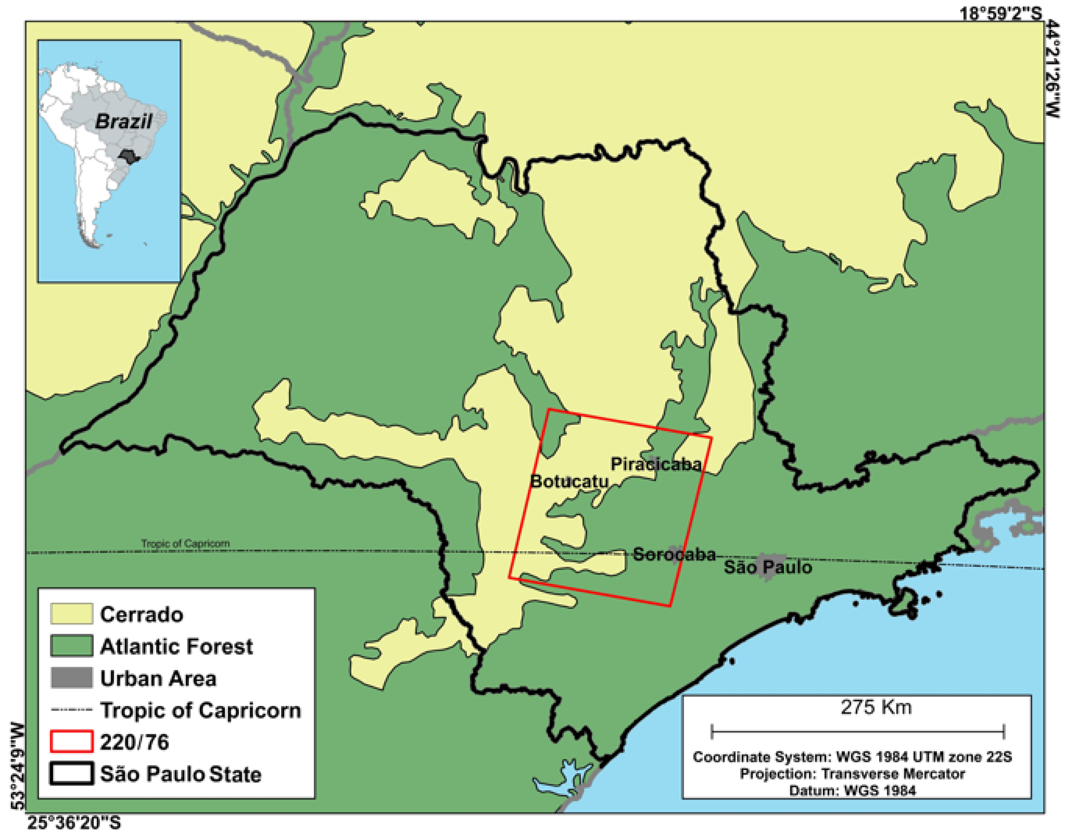
2.1. Study Area

The study area comprises 25,286 km² and corresponds to the common area of the Landsat worldwide reference system 2 (WRS2) 220/76 scenes, including 82 municipalities from 14 different micro regions in the center-south portion of the São Paulo State, (Figure 1). The Portuguese occupation of the region began in colonial times with private and Crown-sponsored expeditions that penetrated the hinterlands looking for precious metals and attempting to enslave native inhabitants. Iron ore exploitation, the foundation of some villages to support expeditions, and the expansion of coffee plantation and railway construction in the late 1800s were at the origin of some pioneer settlements that exist until nowadays as some important cities like Sorocaba and Piracicaba [36,37,38,39]. The last demographic censuses report that approximately 3.8 million people live in the region, and an annual gross domestic product (GDP) of approximately US$ 25.7 billion was registered in 2010 [39,40,41,42].
The major geomorphological units in the study area comprise a central part with slopes ranging from 10 to 20% and altitudes varying from 500 to 650 m. Moreover, some plateaus and steeper Cuestas are found in the northern and southern parts of the study area where elevations reach up to 900 m [43,44,45]. The region was originally covered mostly by interior Atlantic Forest areas, characterized by seasonal semideciduous forests with dense tree cover in which 20% to 50% of the trees defoliate in the dry season [46,47,48].

2.2. Materials

2.2.1. Landsat Images

Landsat thematic mapper (TM) and operational land imager (OLI) images were downloaded from the global visualization viewer (GloVis) (https://glovis.usgs.gov/) platform (Table 1) in L2 surface reflectance level [49] (Table 1). Additionally, Landsat multispectral scanner (MSS) images from 1973 and 1981 were used to visually confirm the presence of large forest remnants mapped by our supervised classification of LULCC processes.

2.2.2. Census Data

Data from the 1995–1996 and the 2006 agricultural censuses and the 2000 and 2010 demographic censuses were obtained from the Brazilian Institute for Geography and Statistics (Instituto Brasileiro de Geografia e Estatística, IBGE) dataset available on http://www2.sidra.ibge.gov.br/. Census statistics included the following variables: sugarcane yield and area; pasture area; urban and rural population; income; planted area of orange, lemon, lime, and tangerines; milk production; and forestry products, such as eucalyptus seedlings; and destination of timber. The comparison between the censuses considered all the municipalities located within the study area [12,41,50].

2.2.3. Ancillary Data

A drainage network map was obtained from the São Paulo State Coordination of Environmental Planning database available online at http://www.ambiente.sp.gov.br/cpla/cessao-de-dados/ [51], and was used to calculate the distance of forest fragments to the nearest river. High-resolution Google Earth images were used to elucidate doubts regarding classification and mapping forest areas. These images were useful in cases where no field data were available. Maps from the CANASAT project (http://www.dsr.inpe.br/laf/canasat/) were obtained to evaluate sugarcane expansion in the study area. This project mapped the sugarcane expansion and land use change in the São Paulo state as a result of an increase in the demand for ethanol, using Landsat type remotely sensed data in the 2003–2013 period [52].

2.3. Methods

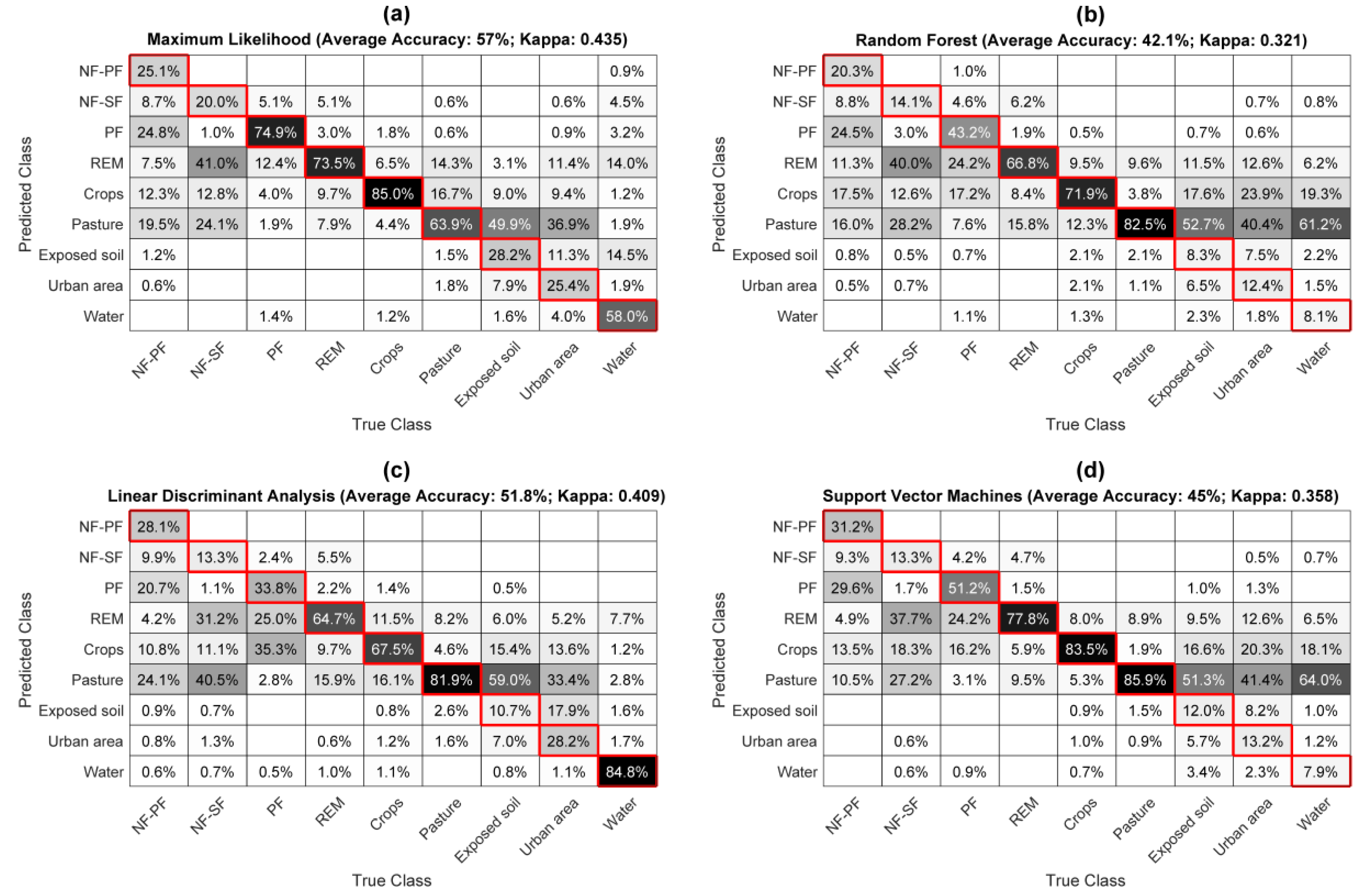
2.3.1. Production of the Forest Transition Map

Supervised classification of LULCC transitions was performed for imagery from periods I and II to identify changes in forest cover. The following transition classes were selected: (i) non-forest to planted forest (newly planted forest, NF-PF); (ii) non-forest to secondary forest (NF-SF); (iii) planted forest (planted forest, PF); and (iv) forest remnants (REM). Non-forest areas (pastures, crops, bare soil, water bodies, and urban areas) as well as areas of planted and secondary forests were identified based on their spectral signatures and landscape patterns, such as shape, texture, and context. Forest remnants were considered as forest fragments greater than 1 ha that showed forest spectral response in all images of the dataset including MSS images. Representative pixels of each transition class were collected from the image pairs of each period to train the maximum likelihood algorithm [53]. Then, the trained model was used to classify the entire Landsat scenes. The resulting classification maps were composed of nine classes (i.e., NF-PF, NF-SF, PF, REM, pastures, crops, bare soil, water bodies, and urban areas). Classification was performed using TM and OLI bands centered at 660 nm (RED), 830 nm (NIR) and 1650 nm (SWIR-1). The combination of these bands with the maximum likelihood algorithm provided the best results in preliminary tests (see Appendix A). As we were interested to map changes in the forest cover, non-forest areas (i.e., pastures, crops, bare soil, water bodies, and urban areas) were excluded. Finally, the forest transition maps of each period were manually edited to eliminate confusion between the forest classes, which occurred mainly between NF-SF and REM (see Figure A2a).
To assess the classification accuracy, the transition map of each period was compared to validation maps produced for 100 randomly selected 1 × 1 km areas and four randomly selected 25 × 25 km areas. The validation maps were produced by visual interpretation of forest areas (including the NF-PF, NF-SF, PF, and REM classes) using TM images, Google Earth high resolution images and information collected during field work. The Kappa coefficient of agreement [54] as well as quantity and allocation disagreement metrics proposed by [55] were computed to assess the classification results.

2.3.2. Census Analysis

Analysis of census data was performed at the municipality level for both the 1995/96 and the 2006 agricultural censuses and for the 1991, 2000, and 2010 demographic censuses. The area of the most important perennial and annual crops in the study site was identified, which would include sugarcane, orange, lemon, lime, and tangerine. Agricultural census also provided statistics for forestry products, including the quantity of eucalyptus seedlings, firewood and timber for the production of paper; and livestock statistics, including stocking rates, milk production, and sugarcane for animal feed. Total population data were retained for the 1991, 2000, and 2010 demographic censuses, and the average income in urban and rural areas based for the 2000 and 2010 censuses.

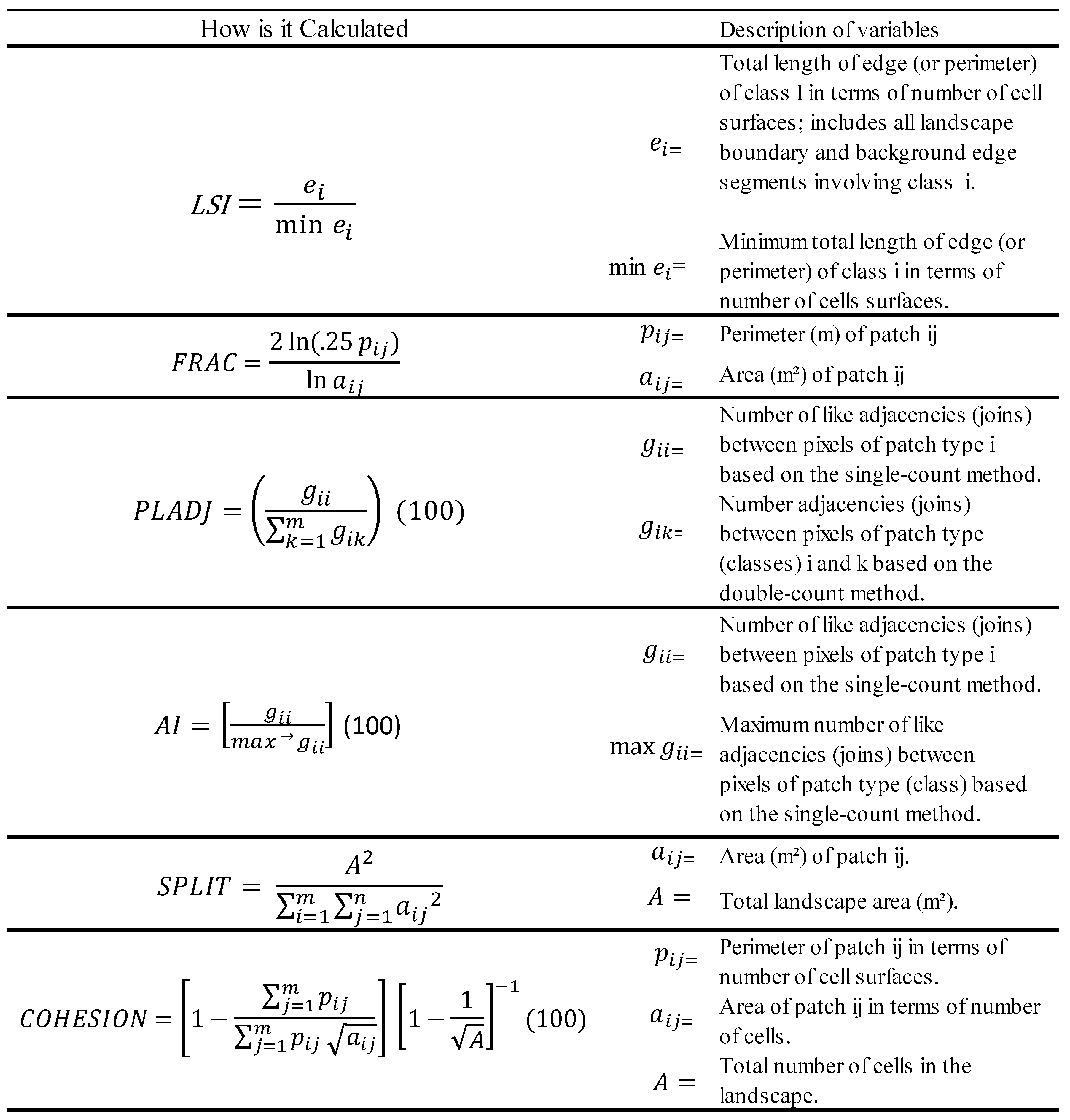
2.3.3. Calculation of Landscape Metric Indices

Landscape metrics were calculated using the ‘spatialEco’ R package [56], which is based on the Fragstats software [57]. Of the great variety of Landscape metrics, the metrics presented on Table 2 give support to the discussion of connectedness, shape, and aggregation of a landscape fragments. The forest remnants map of each period (already converted into binary images) was used to compute six landscape metrics, Table 2. Additionally, the distance to the nearest river and to the nearest fragment edge was calculated for each fragment as well as the total area of forest remnants and regeneration fragments.

3. Results

3.1. Changes in Forest Cover in the Period of Study

The Kappa coefficients of agreement were estimated as 0.668 and 0.654 for periods I and II, respectively, indicating a substantial agreement between ground collected data and classification results [58,59]. In terms of quantity and allocation disagreement, the values were 13.5% and 3.6% for period I; and 10.8% and 4.7% for period II. Moreover, an average accuracy of 82.8% and 84.4% were achieved for period I and II, respectively (Figure 2).
The forest transition maps for periods I (1995–2005) and II (2006–2013) are presented in Figure 3a and Figure 4a, respectively. The areas of the 1995–2005 map show that about 19.9% (502,896 ha) of the study area was covered with forests in period I, and 23.6% (595,918 ha) in period II (Table 3). REM (Figure 3e and Figure 4e) accounted for 15.6% of the in period I and 15.8% in period II. NF-SF (Figure 3c and Figure 4c) accounted for 0.16% in the first period, and 0.07% in the second, totaling 0.23% of the forest cover. NPF (Figure 2d and Figure 3d) accounted for 1.38% and 3.33% during period I and II, respectively.

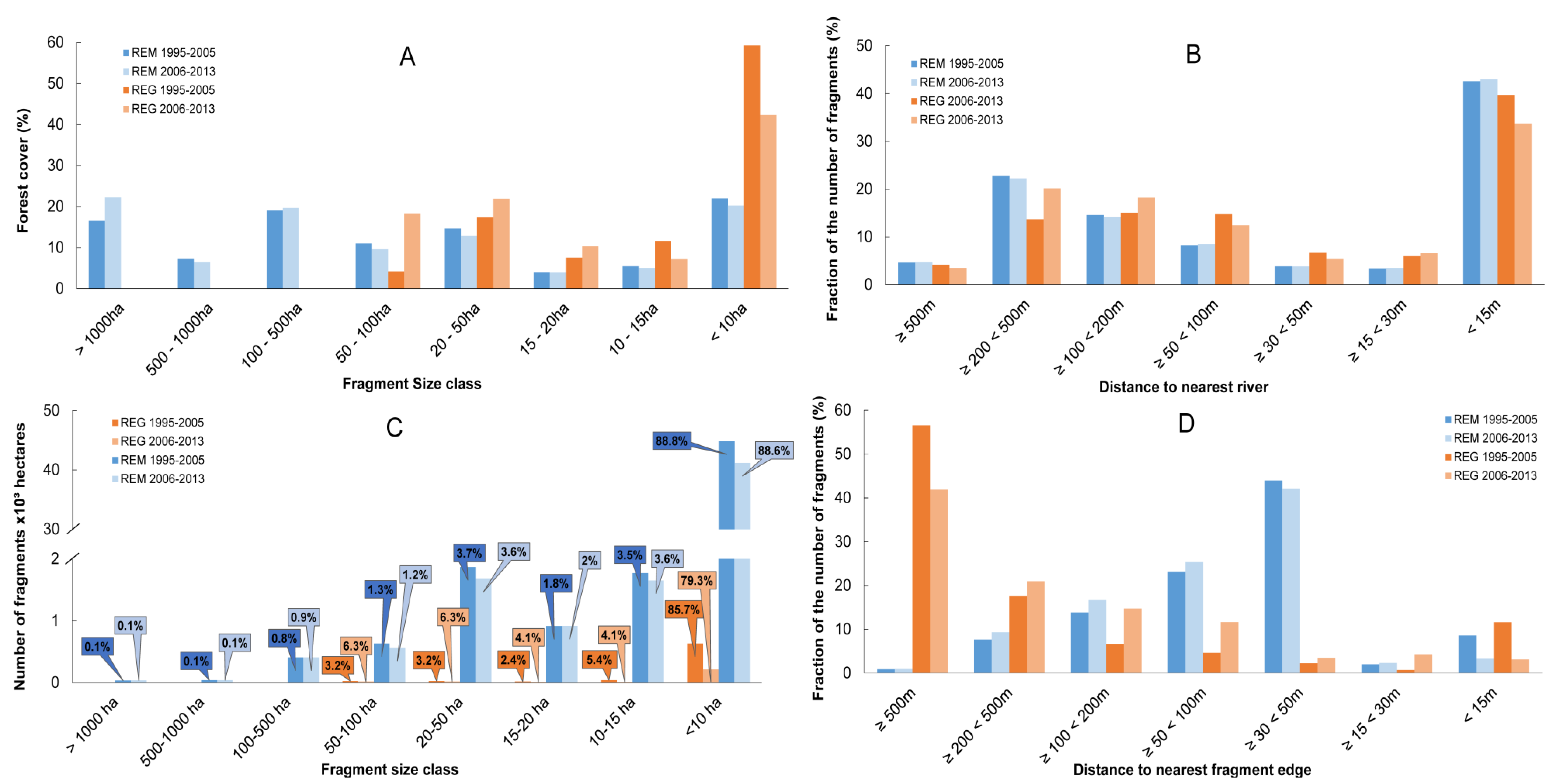
3.2. Landscape Metrics and Isolation of Patches

Landscape metrics for the forest remnants and secondary forest fragments are presented in Table 4, while the distance to the nearest edge (isolation) and to the nearest river for both forest remnants and regeneration fragments are presented in Figure 5.
Considering that the farther are the values from 1 in the LSI index, the more irregular and disaggregated are the fragments [60], the decrease in LSI shown in Table 4 indicate that the fragments tended to be less irregular and more aggregated. This result corroborates that of FRAC, which predicts that the closer to 1, the simpler the patches [60]. Considering the PLADJ, there was the relatively modest increase of 0.03% during the periods, may suggest that there are probably more side-by-side patches. The increase in the AI index complies with the increase in PLADJ, as this index shows that the closer to 100, the more aggregated the patches. There was a decrease in the SPLIT index, which means that the landscape is becoming less subdivided, i.e., that the total number of smaller patches decreased from one period to another. This agrees with the observed increase of 0.05% in connectivity (PC).
Most of forest regeneration was found as fragments < 10 ha, 59.2% and 42.3% for periods I and II, respectively (Figure 5a). The same applies for the total number of forest fragments, in which 85.7% and 79.3% in periods I and II are < 10 ha (Figure 5c). For the forest remnant class, most of the fragments are also < 10 ha in both periods (Figure 5c), but only comprise 22% and 20.2% percent of the total forest cover in periods I and II (Figure 5a), indicating that the forest cover is fairly distributed among the other classes. Fragments > 1000 ha represent 16.6% and 22.2% in periods I and II, and fragments with 100–500 ha comprehend 19.1% and 19.6% of the total forest cover, respectively (Figure 5a).
As for the distance to the nearest river, the majority of both remnants and regeneration fragments are within < 15 m from rivers (Figure 5b), but there are a considerable amount of fragments about 100–500 m distant, 37.4% and 36.4% for remnants and 28.6% and 38.4% for regeneration in periods I and II, respectively. Observing the distance to the nearest fragment edge in Figure 5d, a great extent of the regeneration fragments is 500 m distance from each other, whereas for remnants, most are 30 to 50 m distant in periods I and II, respectively.

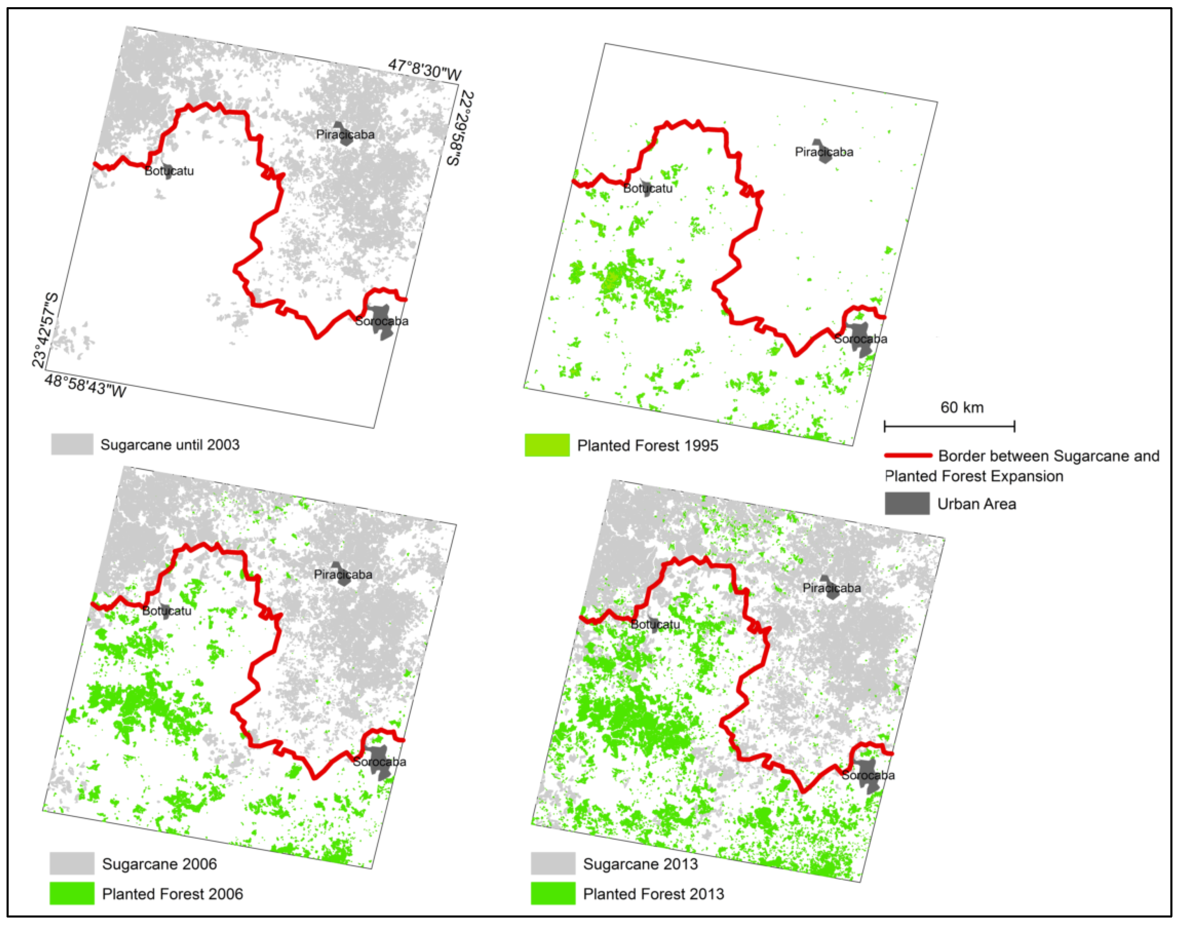
3.3. Forest Transition and Land Use Changes

Data from the 1995/96 and the 2006 Agricultural Censuses [12,13] showed a considerable increase in sugarcane and cellulose production concomitant with a decrease in milk production and the area of citrus (orange, lemon, and lime) (Table 5). Sugarcane production increased 29.9% from 1995 to 2006 in the municipalities within the study area, with sugarcane production attained 2.2 ×10⁷ tons in 2006. Interestingly, the amount of sugarcane used in animal feed decreased 35.1% [12,13]. The area occupied with sugarcane in 1995 was 3.4 × 10⁵ ha and in 2006 it increased 9.7% (i.e., 3.7 × 10⁵ ha).
As census data were not available for period II, we used the CANASAT maps [52] to measure the increase in sugarcane planted area between 2003 and 2013. In 2006, the estimated area occupied with sugarcane was 4.6 × 10⁵ ha, a difference of 22% from that reported in the 2006 census [13] for the same year. CANASAT and census sugarcane planted area differences steams from methodological differences. CANASAT uses satellite imagery and visual interpretation to map sugarcane area, whereas the census only reports what landowners report about their properties. Between 2003 and 2006, sugarcane planted area increased by 14%. This increase was steady and peaked in 2009 with 5.3 × 10⁵ ha. After this year, the area decreased, but continued to be higher than the 2003 values by 26.5%. A total of 1.1 × 10⁵ ha of land was converted to sugarcane, representing 4.3% of the study area.
The map on Figure 6 shows the expansion of sugarcane and planted forest within the study area. The areas used for sugarcane production are concentrated in the north, near the Botucatu municipality, and northeast, around the Piracicaba municipality. Most of the expansion occurred near the areas already destined to sugarcane production, but some degree of expansion was also observed in the direction of the southeast flank of the study area. Concurrently, the expansion of planted forest occurred mainly in the south and southwestern portion.
As for the forest sector, in Table 5, census data showed an increase of 590% in the production of eucalyptus seedlings and 265% in firewood, from 1995 to 2006 [12,13], while the production of wood for paper increased 333%. The censuses of 1995 and 2006 did not record the area of planted forest in hectares for comparison purposes. Still, these results corroborate the increase in area of planted forest observed with remote sensing data during the same period. By 2006, the area occupied with reforestation increased 56% when compared to 1995. In addition, from 1995 to 2013, there was a 180% increase in the area covered with planted forest, which means 1.25 × 10⁵ ha of non-forest areas converted to forest plantations reaching 4.94% of the study area.
Census statistics for citrus shows that citrus harvested area decreased 32.4%, from 6.2 × 10⁴ ha to 4.2 × 10⁴ ha between the two surveys, while the total area of orange production decreased 28.48% (Table 5). At the same time, it could be noted that further analysis showed that the production of citrus in smaller agricultural properties (<10 ha) increased by 65%. Also, in the case of lemon, an overall decrease of 76.6%, was accompanied by a 187% increase among smaller properties 187%, from 31 ha to 89 ha. The production of bergamot/tangerine decreased by 76%, with the production in smaller properties (<5 ha) increasing by 408%, from 51 ha to 239 ha. These results indicate that the production of citrus in larger areas might have been allocated to other areas in the State, and that small holders are partially responsible for keeping the activity, at least for the first period of analysis.
The last two categories analyzed were milk production and pasture area (Table 5). Milk production decreased 23.6% in the area from 1995 to 2006, indicating that the amount and the area destined for dairy cattle decreased. The same occurred to the area of pasture, which decreased 23% from the first period to the second, representing a decrease in area of 2.1 × 10⁵ ha.
Analysis of the demographic censuses showed that there was a decrease of 21.2% in rural population from 1995 to 2010 and an increase of 25.6% in the urban population. Rural areas lost 7.1 × 10⁴ inhabitants and the urban areas gained 7.1 × 10⁵ inhabitants, a value ten-fold greater than the loss registered in rural areas. In the period of 2000 to 2010, average income in urban areas increased 86% from R$ 1152.6 to R$ 2144.3; and in rural areas 98.6%, from R$ 886.8 to R$ 1721.2. The difference of income between urban and rural inhabitants in 2000 was 23%, increasing to 24.6% in 2010.

4. Discussion

The transition from non-forest to secondary forest (NF-SF) throughout the 1995–2013 period accounted for 6.2 × 10³ ha, representing a smaller fraction of the total forest cover changes. At the same time, gains in commercially planted forests (NF-PF) reached 1.26 × 10⁵ ha representing 21% of the forest cover, demonstrating that commercial forest plantations contributed to most of the increase in forest cover. These dynamics are different from that reported by [16] in the west portion of São Paulo State (Presidente Prudente mesoregion), where 2910 ha of secondary forest gains and 330 ha of commercial forest plantations were estimated for the 1986–2009 period, accompanied by a large, 200% increase in sugarcane area. Sugarcane expansion appears to be the leading driver of LULCC in the Presidente Prudente mesoregion [16], whereas for the study area (Sorocaba, Itapetininga, and Piracicaba region), both sugarcane and the forest sectors coexist as important land use systems. This indicates that whatever the processes associated with the possible occurrence of a forest transition, they may be also associated with different contexts even in highly urbanized and more developed areas of the State of São Paulo.
In general, both sugarcane production and commercial forest plantations appear to have been important drivers of LULCC in other areas as well. According to Silva [61], planted forest production in Brazil increased 145% between 1990 and 2010. In 2005, the area covered with planted forest in the São Paulo State was near 9.5 × 10⁵ ha, reaching approximately 11.8 × 10⁵ ha in 2013 [62,63]. Considering the 2.3 × 10⁵ ha from 2005 to 2013 reported in this study, it is possible that nearly half of it may have happened within the present study area. Finally, as the average return on assets from Brazilian commercial forest plantations, as measured by the IRT-Pöyry company, was 7.3% year−1 between 2000 and 2012 [62] suggests that the good profitability from this sector may be driving the considerable forest expansion within the study area.
These findings corroborate with those of [64] that reported an increase of 4.8% in the area of reforestation in the Upper Uruguay Basin, and with [18] and [65] that observed a relative forest cover net change increase of 74% between 1985 and 2011 (from 269 × 103 ha to 470 × 103 ha) in the Paraíba Valley, with an area covered by eucalyptus increasing from 37.5 × 10³ ha to 86.3 × 10³ ha.
The Kappa values of 0.62 and 0.63 in periods I and II, respectively, is lower than the ones found in other studies, such as in [66], but still good according to the criteria used in the literature [58,59]. Furthermore, areas of forest physiognomy, such as planted forests, secondary forest, and primary forest are complex to differentiate due to its spectral similarities. As for the specific problem of forest conservation in the study area, it is noteworthy that the observation of only 15% of forest cover indicates that the 20% forest conservation mandated by the Brazilian Forest Code (Law 12.651/12) has been mostly not enforced [67]. At the same time, the landscape metrics indexes point to an increase in connectivity and proximity among the patches, suggesting that enforcing mandatory preservation of riparian vegetation may improve overall patch connectivity and mitigate landscape fragmentation.
Results from analysis of censuses statistics generally agree with those of [16] that have also found a decrease in milk production and in pasture area and an increase in sugarcane production in the region of Presidente Prudente. These results are also similar with those found by [15], where the expansion of sugarcane in the State of São Paulo poses a conflict over land use, since sugarcane expansion occurred on pasture areas, especially cultivated pasture, and temporary and permanent crops from 1995 to 2013. The decrease in cultivated pasture area within the scene was 56%, and the reduction in permanent crops—such as orange, tangerine, and lime—was 32.4%.
Overall, observed forest transition in the study area has been largely influenced by the forest sector which accounts for most of forest area increase, possibly due to a combination of the ‘forest scarcity path’ and the ‘economic development path’ [23]. There are two key factors found in the census analysis that corroborate with the idea of an ‘economic development path’. The first is related to loss of rural population to urban centers seeking better paying positions, resulting in a relative shortage in labor force followed by rural wage increase, making agricultural activity in remote areas unprofitable. As a result, fallow land, pasture, and some crops may be left for forest regeneration. Even though monthly average income in rural areas increased more than urban areas’ income by 12%, rural areas lost 21.2% of their population from 1991 to 2010. The second factor is related to the increase in monthly average income in rural areas, which according to [68], may be related to the decrease of overall forest degradation. As for the ‘forest scarcity path’, the increase in forest plantation and its products in recent years have been providing timber for the national and international markets, taking out pressure from the remaining original forest cover.

5. Conclusions

This paper investigated the hypothesis of a forest transition underway and its association to large-scale changes in agricultural production in an area in the south-central portion of the State of São Paulo, Brazil. Results showed that the total area covered with forests increased by nearly 30% from 1995 to 2013, indicating a relatively important forest transition in comparison to other areas (e.g., [16]). Yet, this increase can be mainly explained by the expansion of commercial forest plantations in the region, with a minor increase in secondary forests, which agrees with LULCC dynamics reported in other areas of the state (e.g., [18]). Secondly, combining the census data with the results from image classification suggested the occurrence of two major agricultural production systems in the study area, sugarcane and forest plantation. In addition, the analysis of landscape metrics showed that the region of study presented increased connectivity in certain areas with a majority of forest remnants and regeneration fragments within the 50 m from the nearest rivers.
During the development of this study, the process of mapping and validating transition classes proved to be quite challenging due to both spectral confusion and the relatively small size of secondary forest patches, and emphasized that attention must be paid to the selection of the best spectral bands, its quantity, and to detailed validation work. Spectral confusion could be minimized by including spectral bands from as many years as possible. Constant checking of data from the imagery time series was also crucial for the validation of forest transitions, and ameliorating the knowledge about the spectral response of the different land uses.
The integration of remote sensing and census data allowed us to understand the undergoing LULCC processes within the study area. In addition, some changes reported in the censuses, such as the increase in sugarcane production and the increase in planted forest area, were possible to assess using remote sensing data. However, it was not possible to estimate the amount of pasture land that was transformed in planted forest or sugarcane, nor the conversion of citrus areas to other uses; therefore, it is recommended that further studies in this area investigate these transitions, and more sophisticated analyses integrate remotely sensed data and agricultural statistics. The findings regarding landscape metrics could be used to a certain extent to provide subsidies for conservation policies, in particular, in riparian zones. As a final remark, understanding large scale changes in agriculture was useful to gain knowledge on landscape changes and a possible forest transition.

Author Contributions

Conceptualization, A.L.S. and D.S.A., Methodology, A.L.S., D.S.A., M.P.F.; Software, A.L.S., M.P.F.; Validation, A.L.S., D.S.A. and M.P.F.; Formal Analysis, A.L.S.; Investigation, A.L.S.; Resources, National Institute For Space Research (INPE); Data Curation, A.L.S., D.S.A., M.P.F.; Writing-Original Draft Preparation, A.L.S.; Writing-Review & Editing, A.L.S., D.S.A., M.P.F.; Visualization, A.L.S.; Supervision, A.L.S., D.S.A.; Project Administration, A.L.S.; Funding Acquisition, Coordination for the Improvement of Higher Personnel (CAPES). All authors provided critical feedback and helped shape the research, analysis and manuscript.

Acknowledgments

The authors would like to thank the Coordination for the Improvement of Higher Education Personnel (CAPES) for the scholarship and the grant for field work through the post-graduate program in Remote Sensing at INPE-SJC and Egidio Arai, who kindly offered the CANASAT masks.

Conflicts of Interest

The authors declare no conflict of interest.

Appendix A

Figure A1. Detailed description of how the landscape indices are calculated.
Remotesensing 10 00996 g0a1
A classification experiment was carried out to assess the performance of four statistical machine learning methods. First, we selected 5000 pixels corresponding to each transition class (i.e., NF-PF, NF-SF, PF, REM, pastures, crops, bare soil, water bodies, and urban areas) and trained the maximum likelihood [53] random forest [69] linear discriminant analysis [70] and support vector machines methods [71]. Then, the trained models were applied to classify TM image bands (RED, NIR, and SWIR-1) from period I.
The resulting maps were composed of nine classes from which four (i.e., NF-PF, NF-SF, PF, REM) corresponded to forest areas and five (i.e., pastures, crops, bare soil, water bodies, and urban areas) represented non-forest areas. To perform the accuracy assessment, each classification map was compared to validation maps produced for 100 randomly selected 1 × 1 km areas and four randomly selected 25 × 25 km areas. The use of these 25 × 25 km areas was necessary to assess the accuracy of the NF-SF class, which is composed of small forest patches sparsely distributed over the study area. All image processing was performed in R (http://www.R-project.org/). Parameters of the random forest and support vector machines were tuned prior classification using a grid search strategy on the training set. Support vector machines was used with the radial basis function kernel.
The confusion matrices obtained after comparing the validation and classification maps produced by the four machine learning methods are presented in Figure A2. The maximum likelihood algorithm provided the highest average accuracy (57%) and also the highest Kappa coefficient of agreement (0.435). These results motivated the choice of the maximum likelihood algorithm to map the transition classes over the study area.
Figure A2. Confusion matrices obtained for classification maps produced by (a) maximum likelihood, (b) random forest, (c) linear discriminant analysis, and (d) support vector machines. The diagonal cells (highlighted in red) show the classification accuracy of each transition class, while the off-diagonal cells show the percentage of classification error between classes. Empty white cells refer to less than 0.5% misclassification. NF-PF = non-forest to planted forest; NF-SF = non-forest to secondary forest (successional); PF = conservation of planted forests; REM = conservation of forest remnants.
Remotesensing 10 00996 g0a2

References

  1. Geist, H.J.; Lambin, E.F. What Drives Tropical Deforestation; LUCC Report Series; LUCC International Project Office, Department of Geography, University of Louvain: Leuven, Belgium, 2001; Volume 4, 116p. [Google Scholar]
  2. Lambin, E.F.; Turner, B.L.; Geist, H.J.; Agbola, S.B.; Angelsen, A.; Bruce, J.W.; George, P. The causes of land-use and land-cover change: Moving beyond the myths. Glob. Environ. Chang. 2001, 11, 261–269. [Google Scholar] [CrossRef]
  3. Walker, R.; Solecki, W. Theorizing Land-Cover and Land-Use Change: The Case of the Florida Everglades and Its Degradation. Ann. Assoc. Am. Geogr. 2004, 94, 311–328. [Google Scholar] [CrossRef]
  4. Machado, L. A Fronteira Agrícola na Amazônia Brasileira; Revista Brasileira de Geografia Rio de Janeiro: São Paulo, Brazil, 1992; Volume 54, pp. 1–120. [Google Scholar]
  5. Holanda, S.B.; Eulálio, A.; Ribeiro, L.G. Raízes do Brasil; Companhia das Letras: São Paulo, Brazil, 1995. [Google Scholar]
  6. Moraes, A.C.R. Bases da formação territorial do Brasil. Geografares 2001, 2, 105–113. [Google Scholar] [CrossRef]
  7. Becker, B.K. Geopolítica da Amazônia. Estudos Avançados 2005, 19, 71–86. [Google Scholar] [CrossRef]
  8. Alves, D.S. Science and technology and sustainable development in Brazilian Amazon. In Stability of Tropical Rainforest Margins; Springer: Berlin/Heidelberg, Germany, 2007; pp. 491–510. [Google Scholar]
  9. Dean, W. With Broadax and Firebrand: The Destruction of the Brazilian Atlantic Forest; University of California Press: Oakland, CA, USA, 1997. [Google Scholar]
  10. SOS Atlantic Forest. Annual Report—2015. São Paulo. 2015. Available online: https://www.sosma.org.br/wp-content/uploads/2016/08/RA_SOSMA_2015-Web.pdf (accessed on 17 January 2017).
  11. Machado, L. Limites, Fronteiras e Redes. In Fronteiras e Espaço Global, 1st ed.; AGB: Porto Alegre, Brazil, 1998; pp. 41–49. [Google Scholar]
  12. IBGE. Instituto Brasileiro de Geografia e Estatística. Censo Agropecuário 1995/96. Census of Agriculture. 1995/96. Available online: http://www.sidra.ibge.gov.br/ (accessed on 8 February 2017).
  13. IBGE. Instituto Brasileiro de Geografia e Estatística. Censo Agropecuário 2006. Census of Agriculture; 2006. Available online: http://www.sidra.ibge.gov.br/ (accessed on 8 February 2017).
  14. Adami, M.; Rudorff, B.F.T.; Freitas, R.M.; Aguiar, D.A.; Sugawara, L.M.; Mello, M.P. Remote Sensing Time Series to Evaluate Direct Land Use Change of Recent Expanded Sugarcane Crop in Brazil. Sustainability 2012, 4, 574–585. [Google Scholar] [CrossRef] [Green Version]
  15. Camara, M.R.G.D.; Caldarelli, C.E. Expansão canavieira e o uso da terra no estado de São Paulo. Estudos Avançados 2016, 30, 93–116. [Google Scholar] [CrossRef]
  16. Ferreira, M.P.; Alves, D.S.; Shimabukuro, Y.E. Forest dynamics and land-use transitions in the Brazilian Atlantic Forest: The case of sugarcane expansion. Reg. Environ. Chang. 2015, 15, 365–377. [Google Scholar] [CrossRef]
  17. Lira, P.K.; Tambosi, L.R.; Ewers, R.M.; Metzger, J.P. Land-use and land-cover change in Atlantic Forest landscapes. For. Ecol. Manag. 2012, 278, 80–89. [Google Scholar] [CrossRef]
  18. Silva, R.F.B.; Batistella, M.; Moran, E.F. Drivers of land change: Human-environment interactions and the Atlantic forest transition in the Paraíba Valley, Brazil. Land Use Policy 2016, 58, 133–144. [Google Scholar] [CrossRef]
  19. Rudel, T.K.; Coomes, O.T.; Moran, E.; Achard, F.; Angelsen, A.; Xu, J.; Lambin, E. Forest transitions: Towards a global understanding of land use change. Glob. Environ. Chang. Part A 2005, 15, 23–31. [Google Scholar] [CrossRef]
  20. Finegan, B. Pattern and process in neotropical secondary rain forests: The first 100 years of succession. Trends Ecol. Evol. 1996, 11, 119–124. [Google Scholar] [CrossRef]
  21. Farinaci, J.S.; Ferreira, L.D.C.; Batistella, M. Forest transition and ecological modernization: Eucalyptus forestry beyond good and bad. Ambiente Soc. 2013, 16, 25–46. [Google Scholar] [CrossRef]
  22. Mather, A.S. The forest transition. Area 1992, 24, 367–379. [Google Scholar]
  23. Mather, A.S.; Needle, C.L. The forest transition: A theoretical basis. Area 1998, 30, 117–124. [Google Scholar] [CrossRef]
  24. Farinaci, J.S.; Batistella, M. Variação na cobertura vegetal nativa em São Paulo: Um panorama do conhecimento atual. Revista Árvore 2012, 36, 695–705. [Google Scholar] [CrossRef]
  25. Yeo, I.Y.; Huang, C. Revisiting the forest transition theory with historical records and geospatial data: A case study from Mississippi (USA). Land Use Policy 2013, 32, 1–13. [Google Scholar] [CrossRef]
  26. Walker, R. The scale of forest transition: Amazonia and the Atlantic forests of Brazil. Appl. Geogr. 2012, 32, 12–20. [Google Scholar] [CrossRef]
  27. Groom, G.; Mücher, C.A.; Ihse, M.; Wrbka, T. Remote sensing in landscape ecology: Experiences and perspectives in a European context. Landsc. Ecol. 2006, 21, 391–408. [Google Scholar] [CrossRef]
  28. Newton, A.C.; Hill, R.A.; Echeverría, C.; Golicher, D.; Rey Benayas, J.M.; Cayuela, L.; Hinsley, S.A. Remote sensing and the future of landscape ecology. Prog. Phys. Geogr. 2006, 33, 528–546. [Google Scholar] [CrossRef]
  29. Wu, J. Key concepts and research topics in landscape ecology revisited: 30 years after the Allerton Park workshop. Landsc. Ecol. 2013, 28, 1–11. [Google Scholar] [CrossRef]
  30. Li, X.; Lu, L.; Cheng, G.; Xiao, H. Quantifying landscape structure of the Heihe River Basin, north-west China using FRAGSTATS. J. Arid Environ. 2001, 48, 521–535. [Google Scholar] [CrossRef]
  31. Urban, D.; Keitt, T. Landscape connectivity: A graph-theoretic perspective. Ecology 2001, 82, 1205–1218. [Google Scholar] [CrossRef]
  32. Haila, Y. A conceptual genealogy of fragmentation research: From island biogeography to landscape ecology. Ecol. Appl. 2002, 12, 321–334. [Google Scholar]
  33. Yu, X.; Ng, C. An integrated evaluation of landscape change using remote sensing and landscape metrics: A case study of Panyu, Guangzhou. Int. J. Remote Sens. 2006, 27, 1075–1092. [Google Scholar] [CrossRef]
  34. Brudvig, L.A.; Damschen, E.I.; Tewksbury, J.J.; Haddad, N.M.; Levey, D.J. Landscape connectivity promotes plant biodiversity spillover into non-target habitats. Proc. Natl. Acad. Sci. USA 2009, 106, 9328–9332. [Google Scholar] [CrossRef] [PubMed] [Green Version]
  35. Bleyhl, B.; Baumann, M.; Griffiths, P.; Heidelberg, A.; Manvelyan, K.; Radeloff, V.C.; Kuemmerle, T. Assessing landscape connectivity for large mammals in the Caucasus using Landsat 8 seasonal image composites. Remote Sens. Environ. 2017, 193, 193–203. [Google Scholar] [CrossRef]
  36. Lana, R.C. Da Pedra e Cal ao Intangível: Paisagem cultural e educação patrimonial na região de Sorocaba-SP. In Chão da Terra: Olhares, Reflexões e Perspectivas Geográficas de Sorocaba; CRV: Curitiba, Brazil, 2016; 238p. [Google Scholar]
  37. Benevides, G. Polos de Desenvolvimento e a Constituição do Ambiente Inovador: Uma Análise Sobre a Região de Sorocaba. Doctorate Thesis (Doutorado em administração), Universidade Municipal De São Caetano Do Sul, São Caetano Do Sul, Brasil, 2014; 261p. Available online: http://repositorio.uscs.edu.br/bitstream/123456789/326/2/TESE_Gustavo_Benevides.pdf (accessed on 22 May 2018).
  38. Klein, H.S. A oferta de muares no Brasil central: O mercado de Sorocaba, 1825–1880. Estudos Econômicos 1989, 19, 347–372. [Google Scholar]
  39. IBGE. Instituto Brasileiro de Geografia e Estatística. Censo Demográfico. 2003; Estimativa da População. Available online: http://www2.sidra.ibge.gov.br/bda/acervo (accessed on 1 December 2017).
  40. IBGE. Instituto Brasileiro de Geografia e Estatística. Censo Demográfico. 2007; Estimativa da População. Available online: http://www2.sidra.ibge.gov.br/bda/acervo (accessed on 1 December 2017).
  41. IBGE. Instituto Brasileiro de Geografia e Estatística. Censo Demográfico. 2010; Estimativa da População. Available online: http://www2.sidra.ibge.gov.br/bda/acervo (accessed on 8 January 2018).
  42. IBGE. Instituto Brasileiro de Geografia e Estatística. Censo Demográfico. 2014; Estimativa da População. Available online: http://www2.sidra.ibge.gov.br/bda/acervo (accessed on 10 January 2018).
  43. Ross, J.L.S.; Moroz, I.C. Mapa geomorfológico do estado de São Paulo. Revista do Departamento de Geografia 2011, 10, 41–58. [Google Scholar] [CrossRef]
  44. Oliveira Souza, A.; Arruda, E.M. Anomalias de drenagem no Ribeirão dos Rodrigues: Contribuições sobre a geomorfologia da região de Sorocaba-SP. Revista do Departamento de Geografia 2015, 29, 191–211. [Google Scholar]
  45. Souza, E.P.; Arruda, E.M. A abordagem geossistêmica na compreensão da dinâmica ambiental na bacia hidrográfica do Rio Ipanema, região de Sorocaba-SP. Os Desafios da Geografia Física na Fronteira do Conhecimento 2017, 1, 501–511. [Google Scholar]
  46. Silva, J.M.C.; Castelli Carlos, H.M. Estado da biodiversidade da Mata Atlantica brasileira. In Mata Atlântica: Biodiversidade, Ameaças e Perspectivas; Galindo-Leal, C., Câmara, I.G., Eds.; Fundação SOS Mata Atlântica, Conservação Internacional, Centro de Ciências Aplicadas à Biodiversidade: Belo Horizonte, Brasil, 2005; pp. 43–60. [Google Scholar]
  47. Veloso, H.P.; Rangel Filho, A.L.R.; Lima, J.C.A. Classificação da Vegetação Brasileira Adaptada a um Sistema Universal; Ministério da Economia: Rio de Janeiro, Brazil, 1991.
  48. Available online: http://www3.izabelahendrix.edu.br/ojs/index.php/aic/article/view/530 (accessed on 22 May 2018).
  49. USGS. United States Geological Survey. Landsat 4–7: Surface Reflectance Product Guide. 2017. Available online: https://landsat.usgs.gov/sites/default/files/documents/ledaps_product_guide.pdf (accessed on 17 April 2017).
  50. IBGE. Instituto Brasileiro de Geografia e Estatística. Censo demográfico 2000. Demographical Census; 2000. Available online: http://www.ibge.gov.br/estatistica (accessed on 8 February 2017).
  51. Available online: http://arquivos.ambiente.sp.gov.br/cpla/2013/10/Ficha_Tecnica_Drenagem_070515.pdf (accessed on 6 December 2017).
  52. Rudorff, B.F.T.; Aguiar, D.A.; Silva, W.F.; Sugawara, L.M.; Adami, M.; Moreira, M.A. Studies on the Rapid Expansion of Sugarcane for Ethanol Production in São Paulo State (Brazil) Using Landsat Data. Remote Sens. 2010, 2, 1057–1076. [Google Scholar] [CrossRef] [Green Version]
  53. Tso, B.; Mather, P.M. Classification Methods for Remotely Sensed Data; CRC Press: Boca Raton, FL, USA, 2009. [Google Scholar]
  54. Congalton, R.G. A review of assessing the accuracy of classifications of remotely sensed data. Remote Sens. Environ. 1991, 37, 35–46. [Google Scholar] [CrossRef]
  55. Pontius, R.G., Jr.; Millones, M. Death to Kappa: Birth of quantity disagreement and allocation disagreement for accuracy assessment. Int. J. Remote Sens. 2011, 32, 4407–4429. [Google Scholar] [CrossRef]
  56. Package ‘spatialEco’. Available online: https://cran.r-project.org/web/packages/spatialEco/spatialEco.pdf (accessed on 30 November 2017).
  57. McGarigal, K.; Cushman, S.A.; Neel, M.C.; Ene, E. FRAGSTATS: Spatial Pattern Analysis Program for Categorical Maps; Department of Environmental Conservation, University of Massachusetts: Amherst, MA, USA, 2002. [Google Scholar]
  58. Viera, A.J.; Garrett, J.M. Understanding interobserver agreement: The kappa statistic. Fam. Med. 2005, 37, 360–363. [Google Scholar] [PubMed]
  59. Landis, J.R.; Koch, G.G. The measurement of observer agreement for categorical data. Biometrics 1977, 33, 159–174. [Google Scholar] [CrossRef] [PubMed]
  60. McGarigal, K.; Barbara, J.M. Spatial Pattern Analysis Program for Quantifying Landscape Structure; Gen. Tech. Rep. PNW-GTR-351; US Department of Agriculture, Forest Service, Pacific Northwest Research Station: Washington, DC, USA, 1995.
  61. Silva, B.K.D. Investments in Timberland: Investors\’Strategies and Economic Perspective in Brazil. Ph.D. Thesis, Universidade de São Paulo, São Paulo, Brazil, 2013. [Google Scholar]
  62. ABRAF. Associação Brasileira de Produtores de Florestas Plantadas. Anuário Estatístico; Ano Base 2005; Abraf: Brasília, Brazil, 2006. [Google Scholar]
  63. ABRAF. Associação Brasileira de Produtores de Florestas Plantadas. Anuário Estatístico; Ano Base 2012; Abraf: Brasília, Brazil, 2013. [Google Scholar]
  64. Freitas, M.W.D.; Santos, J.R.; Alves, D.S. Land-use and land-cover change processes in the Upper Uruguay Basin: Linking environmental and socioeconomic variables. Landsc. Ecol. 2013, 28, 311–327. [Google Scholar] [CrossRef]
  65. Silva, R.F.B.; Batistella, M.; Moran, E.F.; Lu, D. Land changes fostering Atlantic forest transition in Brazil: Evidence from the Paraíba Valley. Prof. Geogr. 2017, 69, 80–93. [Google Scholar] [CrossRef]
  66. Müller, H.; Rufin, P.; Griffiths, P.; Siqueira, A.J.B.; Hostert, P. Mining dense Landsat time series for separating cropland and pasture in a heterogeneous Brazilian savanna landscape. Remote Sens. Environ. 2005, 156, 490–499. [Google Scholar] [CrossRef]
  67. Presidência da República. Available online: http://www.planalto.gov.br/ccivil_03/_ato2011-2014/2012/lei/l12651.htm (accessed on 17 January 2018).
  68. Chowdhury, R.R.; Moran, E.F. Turning the curve: A critical review of Kuznets approaches. Appl. Geogr. 2012, 32, 3–11. [Google Scholar] [CrossRef]
  69. Breiman, L. Random forests. Mach. Learn. 2001, 45, 5–32. [Google Scholar] [CrossRef]
  70. Duda, R.O.; Hart, P.E.; Stork, D.H. Pattern Classification, 2nd ed.; Wiley Interscience: New York, NY, USA, 2000. [Google Scholar]
  71. Vapnik, V.N. The Nature of Statistical Learning Theory, 2nd ed.; Springer: New York, NY, USA, 2000. [Google Scholar]
Figure 1. Location of the study area (Landsat WRS2 220/76) shown with the São Paulo State, Brazil, with the main cities (Sorocaba, Piracicaba, and Botucatu) and Atlantic Forest and Cerrado biome limits.
Remotesensing 10 00996 g001
Figure 2. Confusion matrices obtained for forest transition maps produced for (a) period I (1995–2005) and (b) period II (2006–2013). The diagonal cells (highlighted in red) show the classification accuracy of each transition class, while the off-diagonal cells show the percentage of classification error between classes. Empty white cells refer to less than 0.01% misclassification. NF-PF = non-forest to planted forest; NF-SF = non-forest to secondary forest (successional); PF = conservation of planted forests; REM = conservation of forest remnants.
Remotesensing 10 00996 g002
Figure 3. In (A) forest cover transitions map for the 1995–2005 period, with examples of: (B) planted forest (PF); (C) non-forest to secondary forest (NF-SF); (D) non-forest to planted forest (NF-PF); and (E) remnants (REM). (BE) show false color composites RGB 453 of Landsat TM images from 1995, 2000, and 2005.
Remotesensing 10 00996 g003
Figure 4. In (A) forest cover transitions map for the 2006–2013 period, with example of: (B) planted forest (PF); (C) non-forest to secondary forest (NF-SF); (D) non-forest to planted forest (NF-PF); and (E) remnants (REM). (BE) show false color RGB 453 of a Landsat TM images for 2006 and 2009 and RGB 564 of a Landsat OLI of 2013.
Remotesensing 10 00996 g004
Figure 5. Forest regeneration and remnants transition classes’ metrics. (a) Percentage of forest cover per fragment size class. (b) Fraction of the number of fragments (%) according to the distance to the nearest river. (c) Total number of fragments and the corresponding percentage per fragments size class. (d) Percentage of the number of fragments according to the distance to the fragment edge.
Remotesensing 10 00996 g005
Figure 6. Areas of sugarcane (based on CANASAT [53]) and planted forest expansion (mapped in this work) over the study area during the period analyzed.
Remotesensing 10 00996 g006
Table 1. Landsat images used in the study.
Images Used for Forest Change Classification
SensorQuantityDate
Processed
TM32 May 1995
4 April 2005
14 April 2006
OLI16 June 2013
Used for cross-check and validation
TM1424 August 1996
11 August 1997
7 March 1998
2 September1999
29 April 2000
25 October2001
24 July 2002
15 October 2003
30 August 2004
20 June 2007
10 September 2008
24 May 2009
4 February 2010
3 July 2011
Used for fine tuning image processing techniques with field data collected in September 2017
OLI13 September2017
Table 2. Landscape metrics description (From [56]). More information about how the indices are calculated can be found at Appendix A.
IndexDescription
Landscape Shape Index (LSI)A standardized measure of total edge or edge density that adjusts for the size of the landscape (dimensionless)
Mean Frac. Dim Index (FRAC)Mean of fractal dimension index (dimensionless)
Prop Like Adjacencies (PLADJ)Calculated from the adjacency matrix, which shows the frequency with which different pairs of patch types (including like adjacencies between the same patch type) appear side-by-side on the map (measures the degree of aggregation of patch types) (unit: percent).
Aggregation Index (AI)Computed simply as an area-weighted mean class aggregation index, where each class is weighted by its proportional area in the landscape (unit: percent)
Splitting Index (SPLIT)Based on the cumulative patch area distribution and is interpreted as the effective mesh number, or number of patches with a constant patch size when the landscape is subdivided into S patches, where S is the value of the splitting index (dimensionless)
Patch Cohesion Index (PC)Measures the physical connectedness of the corresponding patch type (dimensionless)
Table 3. Areas corresponding to the main forest cover transitions from Figure 2 and Figure 3.
1995–20052006–2013
Process and InitialsArea (103 ha)Fraction of the Study Area (%)Area (103 ha)Fraction of the Study Area (%)
Non-Forest to Planted ForestNF-PF34.91.3884.33.33
Non-Forest to Secondary Forest (successional) NF-SF4.10.161.90.07
Conservation of Planted ForestsPF69.62.75111.04.4
Conservation of Forest RemnantsREM394.115.6398.715.8
All Forested Area 502.919.9595.923.6
Table 4. Landscape metrics for forest remnants and secondary forest patches.
1995–20052006–2013
LSI442.72408.25
FRAC1.121.11
PLADJ0.650.68
AI78.8880.64
SPLIT57,887.2926,246.61
PC9.829.87
Table 5. Sugarcane and agricultural production from Census statistics and sugarcane area from the CANASAT project.
IBGE Censuses Analysis 1995–2006
1995/96 Census2006 CensusChange (%)
Forest Sector
Firewood (thousand m3)8172981265.0%
Paper (thousand m3)11104807333.0%
Eucalyptus Seedlings (×103 units)741551,193590.4%
Sugarcane Sector CANASAT Estimated planted area
Sugarcane (tons)220,556,53528,659,68229.9%20062013
Sugarcane for animal feed (tons)152,56098,935−35.1%
Sugarcane planted area (hectares)343,858377,1129.7%462,409512,567
Permanent Crop Harvested Area
Orange (hectares)57.57741.174−28.5%
Lime (hectares)26.625−81.2%
Lemon (hectares)1.178269−76.6%
Tangerine (hectares)3.9112935−76.1%
Other Variables
Pasture (hectares)910,695701,297−23.0%
Milk Production (liters)150,008,5851.15 × 108−23.6%

