The Potential and Challenges of Using Soil Moisture Active Passive (SMAP) Sea Surface Salinity to Monitor Arctic Ocean Freshwater Changes

 and
and 
Abstract
:
1. Introduction
2. Data
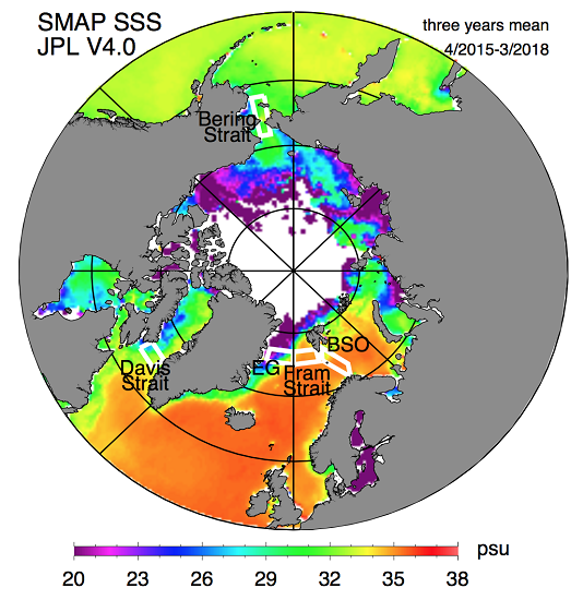
2.1. SMAP SSS
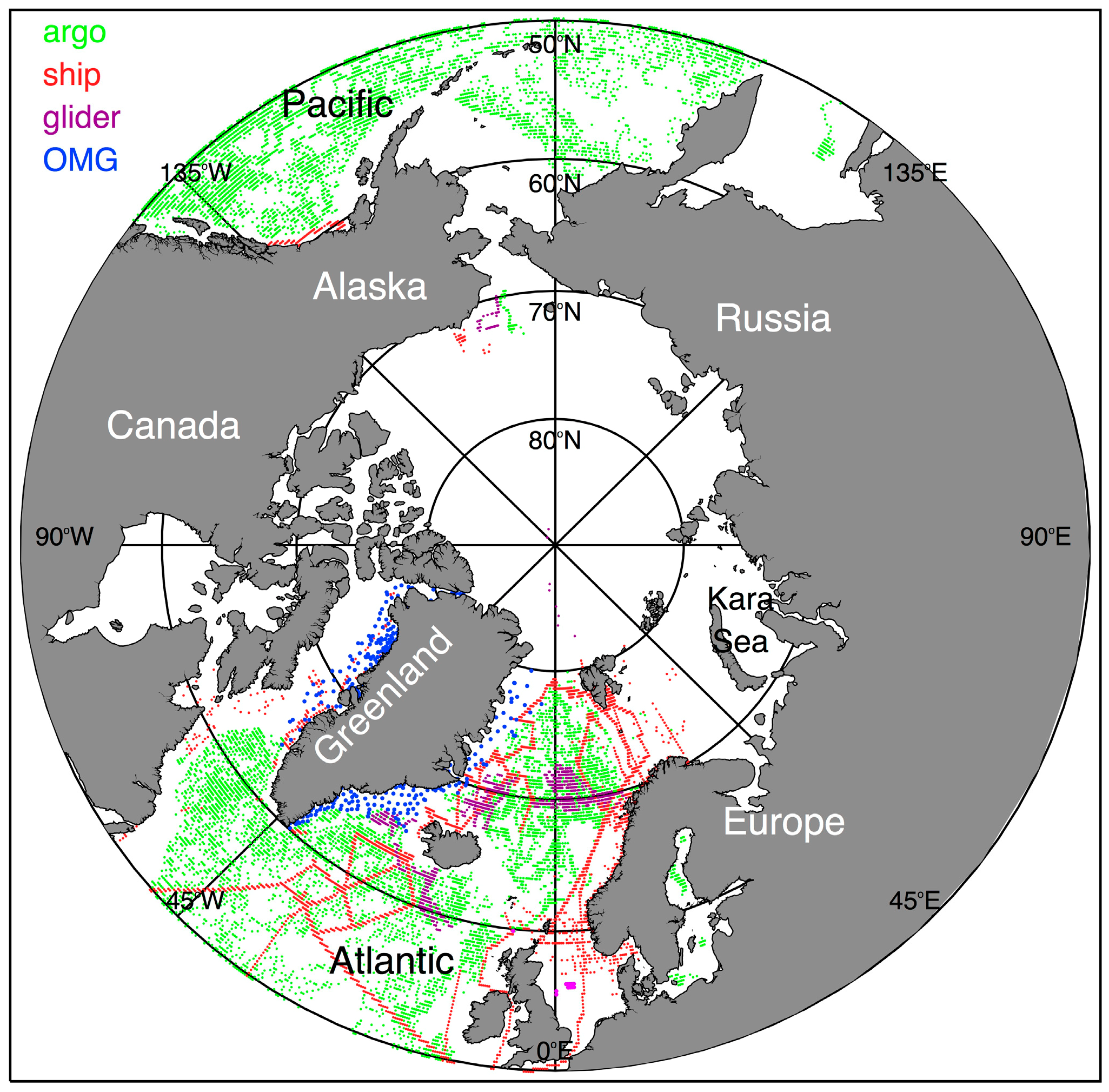
2.2. In Situ Salinity Data
2.3. Sea Ice Concentration
2.4. River Discharge
2.5. Moorings at Arctic Gateways
3. Results
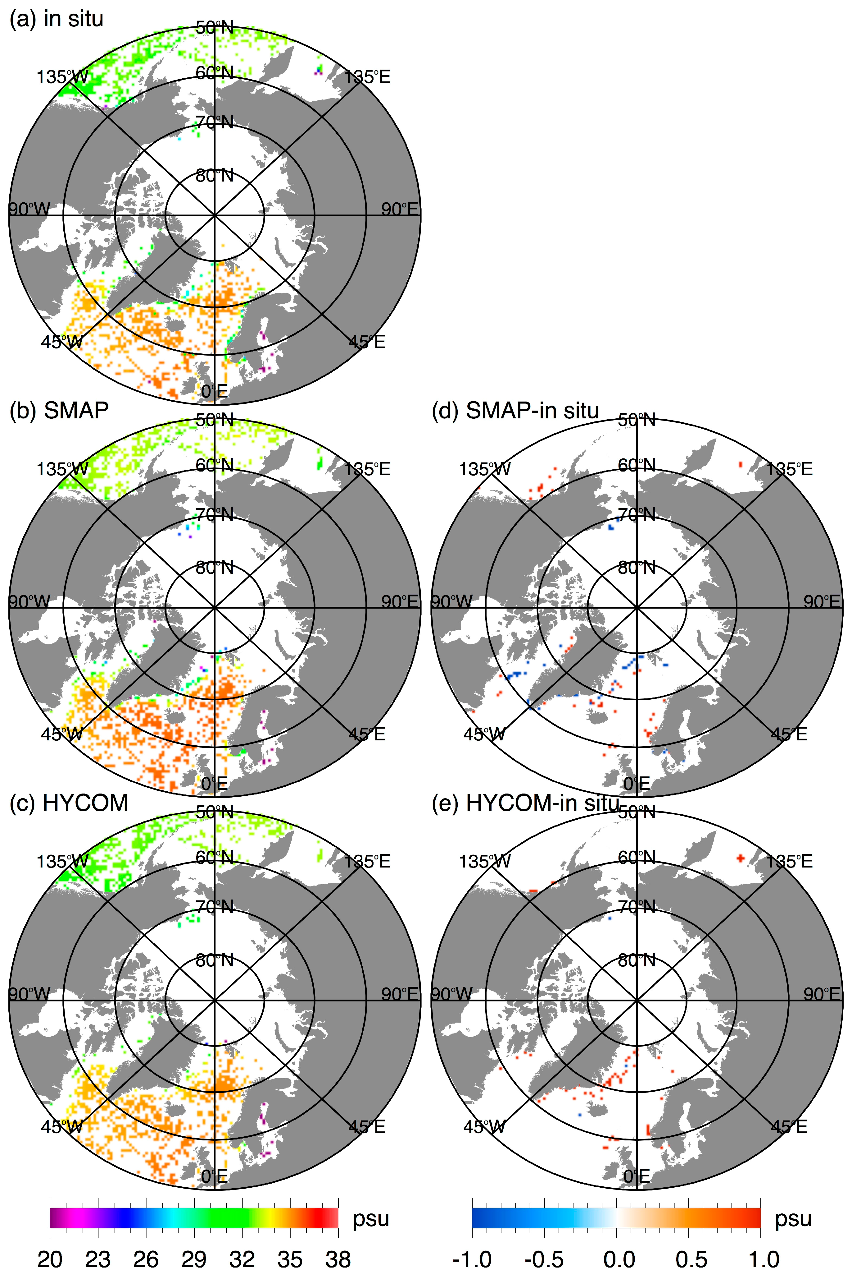
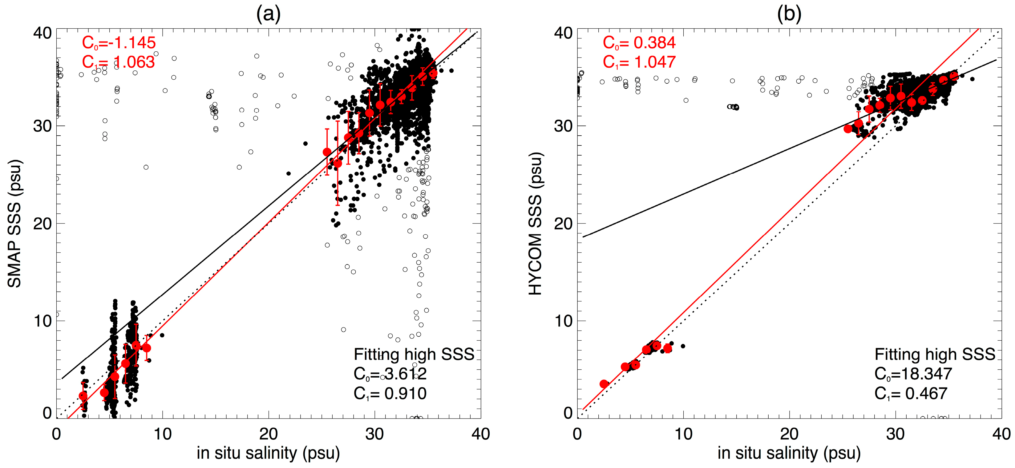
3.1. Validation with In Situ Salinity
3.2. The Arctic Ocean SSS and Sea Ice
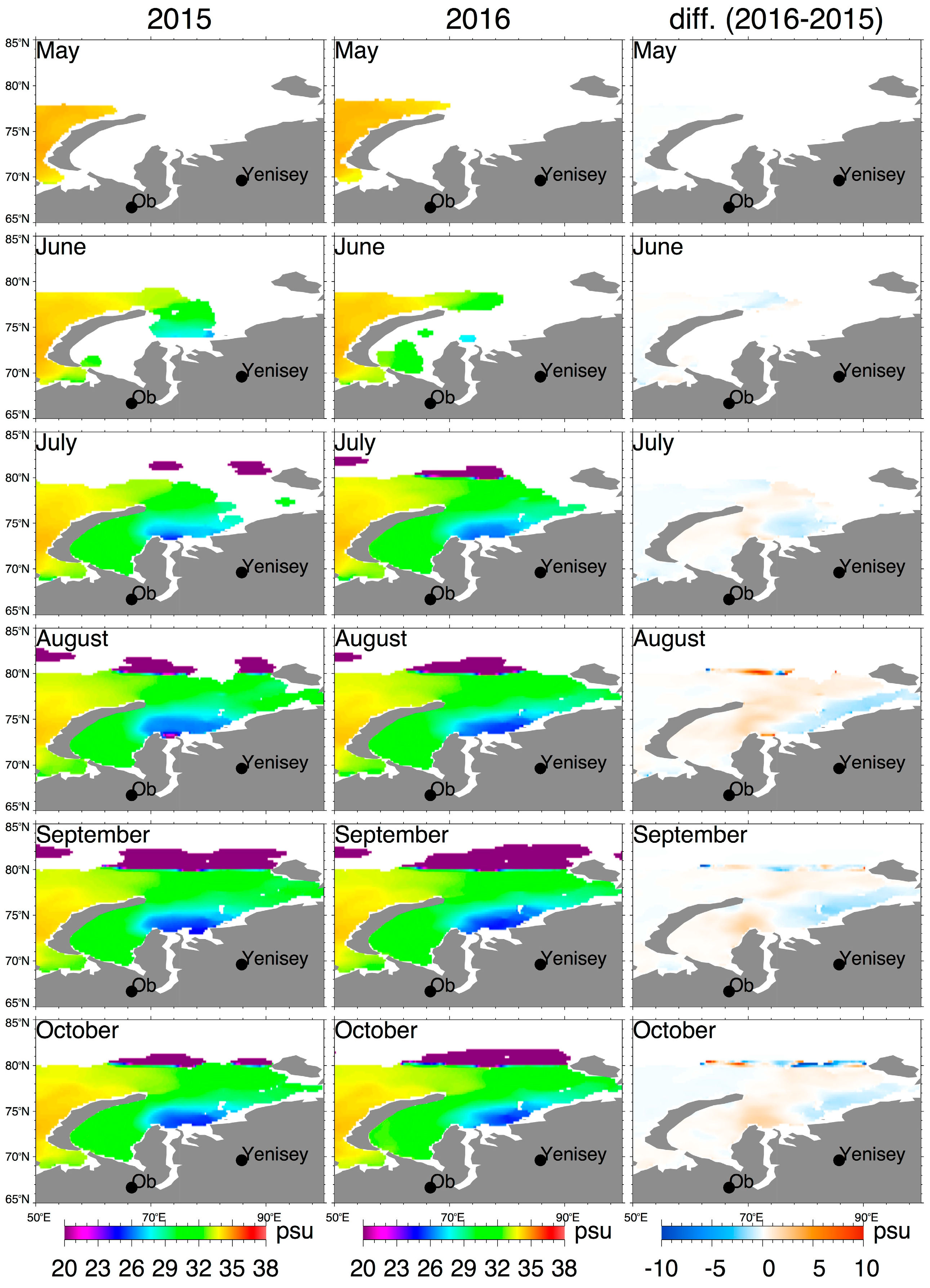
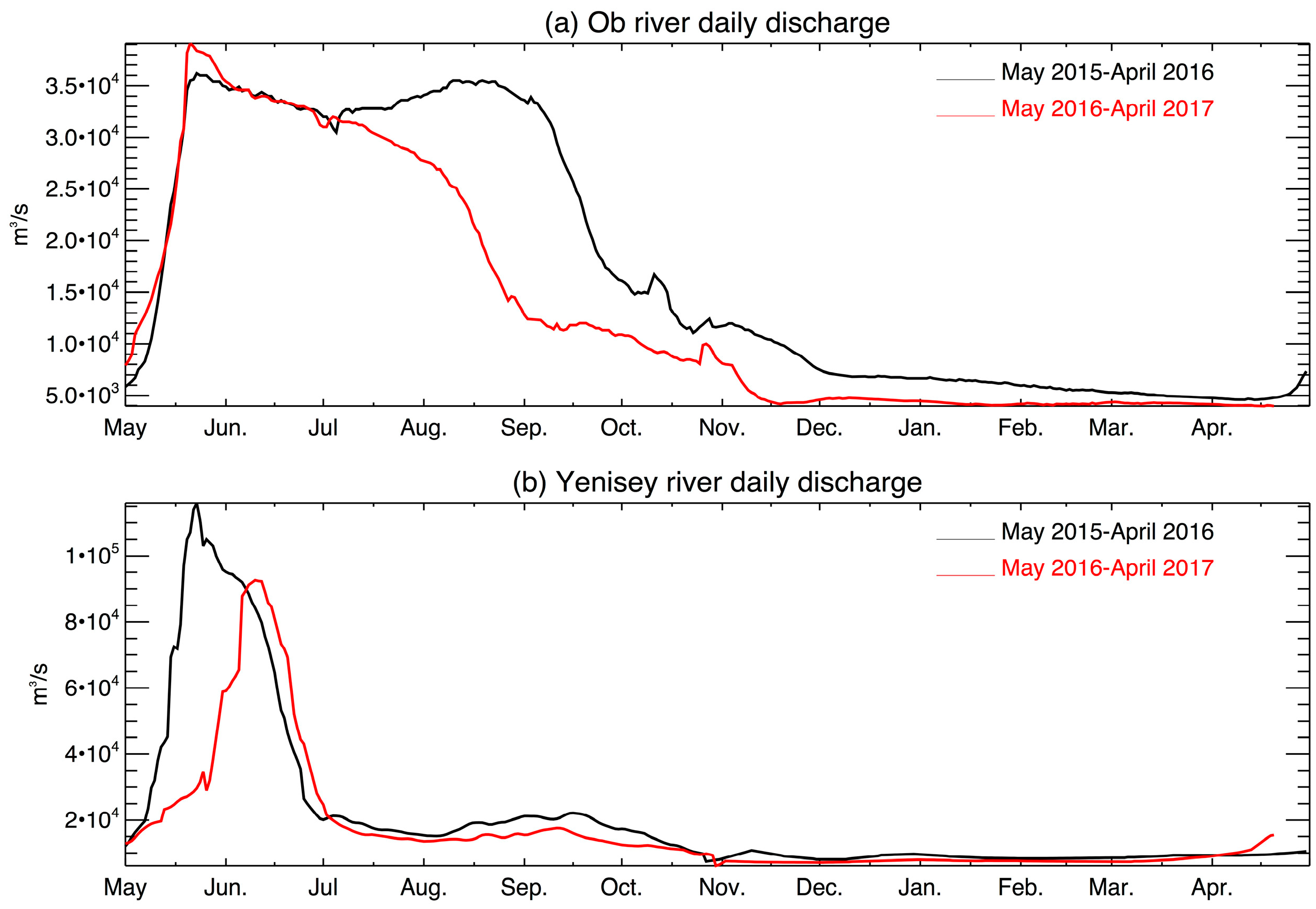
3.3. SSS and River Discharge
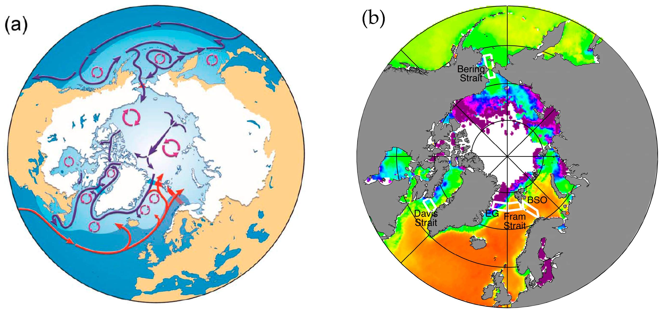
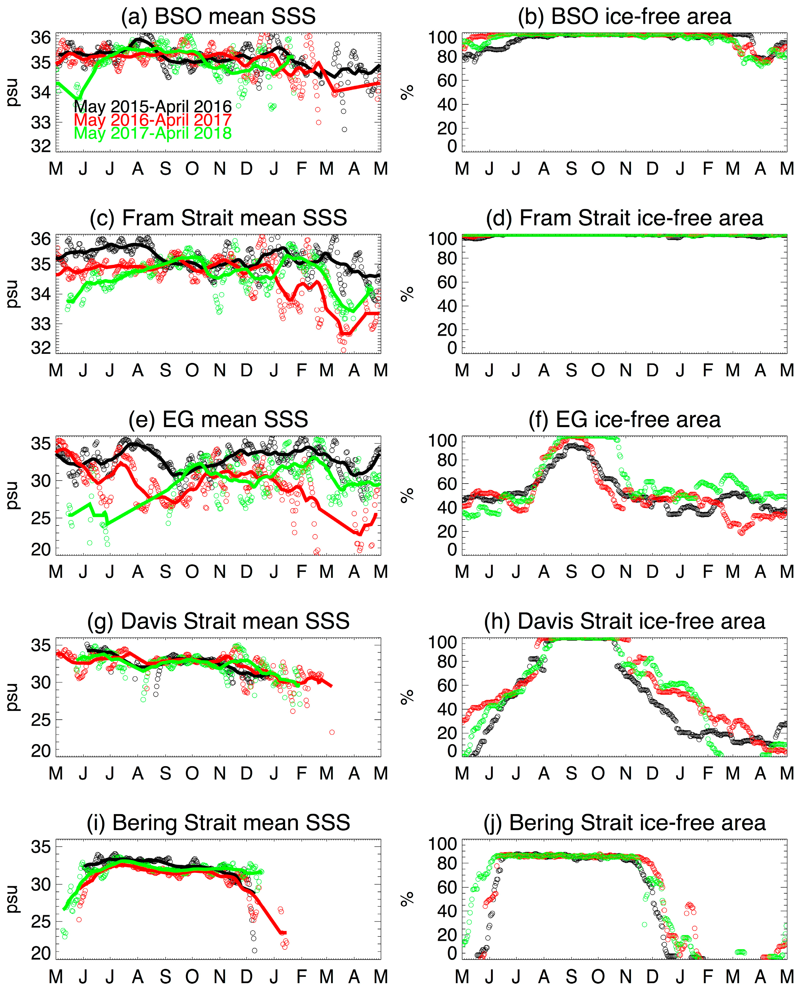
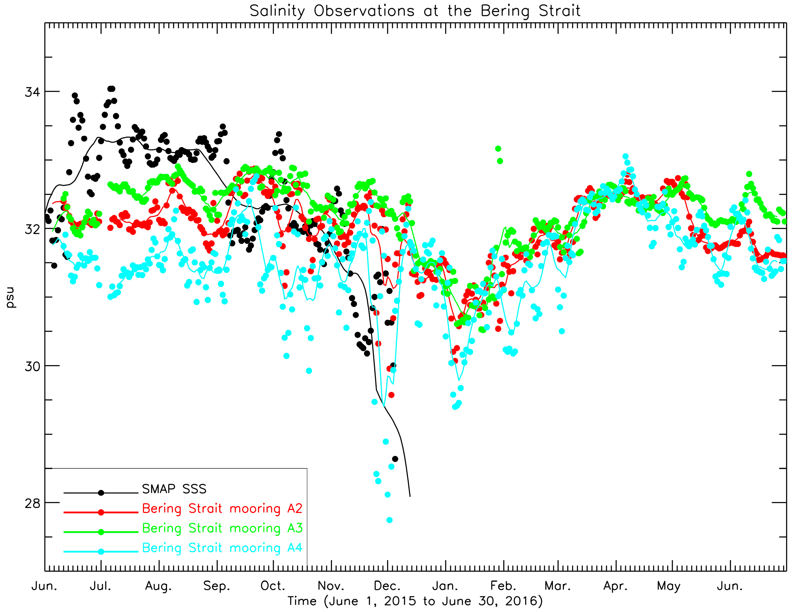
3.4. SSS Variability at Arctic Ocean Gateways
4. Discussion
5. Conclusions
Author Contributions
Acknowledgments
Conflicts of Interest
Abbreviations
| AON | Arctic Observing Network |
| APL | Applied Physics Laboratory |
| Arctic-GRO | Arctic Great River Observatory |
| AXCTD | Airborne eXpandable CTD |
| BSO | The Barents Sea Opening |
| CMEMS | Copernicus Marine Environment Monitoring Service |
| CTD | Conductivity Temperature Depth |
| CONAE | Comision Nacional de Actividades Espaciales |
| ESA | The European Space Agency |
| GOOS | Global Ocean Observing System |
| HYCOM | Hybrid Coordinate Ocean Model |
| INS TAC | In Situ Thematic Assembly Centre |
| JPL | Jet Propulsion Laboratory |
| LUT | look-up-table |
| NASA | The National Aeronautics and Space Administration |
| NCEP | National Centers for Environmental Prediction |
| NRT | near-real-time |
| NSF | The National Science Foundation |
| NSIDC | The National Snow and Ice Data Center |
| OMG | Ocean Melting Greenland |
| PARTNERS | Pan-Arctic River Transport of Nutrients, Organic Matter, and Suspended Sediments |
| PO.DAAC | Physical Oceanography Distributed Active Archive Center |
| RMSD | Root Mean Square Difference |
| ROOS | Regional Ocean Observing System |
| RSS | Remote Sensing System |
| SIC | sea ice concentration |
| SMAP | Soil Moisture Active Passive |
| SMOS | Soil Moisture and Ocean Salinity |
| SSS | sea surface salinity |
| SST | sea surface temperature |
| SWC | salinity-wind-cell |
| TB | brightness temperature |
| TSG | Thermosalinograph |
| USGODAE | The US Global Ocean Data Assimilation Experiment |
| UTC | The Coordinated Universal Time |
| XCTD | eXpendable CTD |
References
- Kwok, R.; Cunningham, G.F.; Wensnahan, M.; Rigor, I.; Zwally, H.J.; Yi, D. Thinning and volume loss of Arctic sea ice: 2003–2008. J. Geophys. Res. 2009, 114, C07005. [Google Scholar] [CrossRef]
- Comiso, J.C. A rapidly decline perennial sea ice cover in the Arctic. Geophys. Res. Lett. 2002, 29, 1956. [Google Scholar] [CrossRef]
- Cavalieri, J.D.; Parkinson, C.L. Arctic sea ice variability and trends. 1979–2010. Cryosphere 2012, 6, 881–889. [Google Scholar] [CrossRef]
- Proshutinsky, A.; Krishfield, R.; Timmemans, M.-L.; Toole, J.; Carmack, E.; McLaughlin, F.; Williams, W.J.; Zimmermann, S.; Itoh, M.; Shimada, K. The Beaufort Gyre Fresh Water Reservior: State and variability from observations. J. Geophys. Res. 2009, 114, C00A10. [Google Scholar] [CrossRef]
- Haine, T.W.N.; Curry, B.; Gerdes, R.; Hansen, E.; Karcher, M.; Lee, C.; Rudels, B.; Spreen, G.; Steur, L.; Stewart, K.D.; et al. Arctic freshwater export: Status, mechanisms, and prospects. Glob. Planet Chang. 2015, 125, 13–35. [Google Scholar] [CrossRef] [Green Version]
- Rage, B.; Karcher, M.; Schauer, U.; Toole, J.; Krishfield, R.; Pisarev, S.; Kauker, F.; Gerdes, R.; Kikuchi, T. An assessment of Arctic Ocean freshwater content changes from the 1990s to 2006–2008. Deep Sea Res. 2011, 58, 173–185. [Google Scholar] [CrossRef] [Green Version]
- McLaughlin, F.A.; Carmack, E.C.; Williams, W.J.; Zimmerman, S.; Shimada, K.; Itoh, M. Joint effects of boundary currents and thermo-haline intrusions on the warming of Atlantic water in the Canada Basin, 1993–2007. J. Geophys. Res. 2009, 114, C00A12. [Google Scholar] [CrossRef]
- Polyakov, I.V.; Pnyushkov, A.V.; Timokhov, T.A. Warming of the intermediate Atlantic Water of the Arctic Ocean in the 2000s. J. Clim. 2012, 25, 8362–8370. [Google Scholar] [CrossRef]
- Rawlins, M.A.; Steele, M.; Holland, M.; Adam, J.; Cherry, J.; Francis, J.; Groisman, P.; Hinzman, L.; Huntington, T.; Kane, D.; et al. Analysis of the Arctic System for Freshwater Cycle Intensification: Observations and Expectations. J. Clim. 2010. [Google Scholar] [CrossRef]
- Willis, J.K.; Rignot, E.; Nerem, R.S.; Lindstrom, E. Introduction to the special issue on ocean-ice interaction. Oceanography 2016, 29, 19–21. [Google Scholar] [CrossRef]
- Fenty, I.; Willis, J.K.; Khazendar, A.; Dinardo, S.; Forsberg, R.; Fukumori, I.; Holland, D.; Jakobsson, M.; Moller, D.; Morison, J.; et al. Oceans Melting Greenland: Early results from NASA’s ocean-ice mission in Greenland. Oceanography 2016, 29, 72–83. [Google Scholar] [CrossRef]
- Prowse, T.; Bring, A.; Mård, J.; Carmack, E. Arctic Freshwater Synthesis: Introduction. J. Geophys. Res. Biogeosci. 2015, 120, 2121–2131. [Google Scholar] [CrossRef] [Green Version]
- Prowse, T.; Bring, A.; Mård, J.; Carmack, E.; Holland, M.; Instanes, A.; Vihma, T.; Wrona, F.J. Arctic Freshwater Synthesis: Summary of key emerging issues. J. Geophys. Res. Biogeosci. 2015, 120, 1887–1893. [Google Scholar] [CrossRef] [Green Version]
- Carmack, C.E.; Yamamoto-Kawai, M.; Haine, T.W.N.; Bacon, S.; Bluhm, B.A.; Lique, C.; Melling, H.; Polyakov, I.V.; Straneo, F.; Timmermans, M.-L. Freshwater and its role in the Arctic Marine System: Sources, disposition, storage, export, and physical and biogeochemical consequences in the Arctic and global oceans. J. Geophys. Res. Biogeosci. 2016, 121. [Google Scholar] [CrossRef]
- Lique, C.; Holland, M.M.; Dibike, Y.B.; Lawrence, D.M.; Screen, J.A. Modeling the Arctic freshwater system and its integration in the global system: Lessons learned and future challenges. J. Geophys. Res. Biogeosci. 2016, 121, 540–566. [Google Scholar] [CrossRef] [Green Version]
- Thomson, J.; Ackley, S.; Girard-Ardhuin, F.; Ardhuin, F.; Babanin, A.; Boutin, G.; Brozena, J.; Cheng, S.; Collins, C.; Doble, M. Overview of the Arctic Sea State and Boundary Layer Physics Program. J. Geophys. Res. Oceans 2018. [Google Scholar] [CrossRef]
- Durack, P.J. Ocean salinity and the global water cycle. Oceanography 2015, 28, 20–31. [Google Scholar] [CrossRef]
- Durack, P.J.; Wijffels, S.E.; Matear, R.J. Ocean Salinities Reveal Strong Global Water Cycle Intensification During 1950 to 2000. Science 2012, 336, 455–458. [Google Scholar] [CrossRef] [PubMed] [Green Version]
- Schmitt, R.W. Salinity and the global water cycle. Oceanography 2008, 21, 12–19. [Google Scholar] [CrossRef]
- Schmitt, R.W. The ocean component of the global water cycle: US National Report to International Union of Geodesy and Geophysics, 1991–1994. Rev. Geophys. 1995, 33 (Suppl. 1), 1395–1409. [Google Scholar] [CrossRef]
- Wijffels, S.E.; Schmitt, R.W.; Bryden, H.L.; Stigebrandt, A. On the transport of fresh water by the oceans. J. Phys. Oceanography 1992, 22, 155–162. [Google Scholar] [CrossRef]
- Timmermans, M.-L.; Proshutinsky, A.; Golubeva, E.; Jackson, J.M.; Krishfield, R.; McCall, M.; Platov, G.; Toole, J.; Williams, W.; Kikuchi, T.; et al. Mechanisms of Pacific Summer Water variability in the Arctic’s Central Canada Basin. J. Geophys. Res. Oceans 2014, 119, 7523–7548. [Google Scholar] [CrossRef]
- Timmermans, M.-L.; Proshutinsky, A.; Krishfield, R.A.; Perovich, D.K.; Richter-Menge, J.A.; Stanton, T.P.; Toole, J.M. Surface freshening in the Arctic Ocean’s Eurasian Basin: An apparent consequence of recent change in the wind-driven circulation. J. Geophys. Res. 2011, 116, C00D03. [Google Scholar] [CrossRef]
- Woodgate, R.A. Increases in the Pacific inflow to the Arctic from 1990 to 2015, and insights into seasonal trends and driving mechanisms from year-round Bering Strait mooring data. Prog. Oceanogr. 2018, 160, 124–154. [Google Scholar] [CrossRef]
- Frajka-Williams, E.; Bamber, J.L.; Våge, K. Greenland melt and the Atlantic meridional overturning circulation. Oceanography 2016, 29, 22–33. [Google Scholar] [CrossRef]
- Yang, Q.; Dixon, T.H.; Myers, P.G.; Bonin, J.; Chambers, D.; van den Broeke, M.R.; Ribergaard, M.H.; Mortensen, J. Recent increases in Arctic freshwater flux affects Labrador Sea convection and Atlantic overturning circulation. Nat. Commun. 2016, 7, 10525. [Google Scholar] [CrossRef] [PubMed] [Green Version]
- Jackson, L.C.; Kahana, R.; Graham, T.; Ringer, M.A.; Woollings, T.; Mecking, J.V.; Wood, R.A. Global and European climate impacts of a slowdown of the AMOC in a high resolution GCM. Clim. Dyn. 2015, 45, 299–316. [Google Scholar] [CrossRef]
- Leuliette, E.W.; Nerem, R.S. Contributions of Greenland and Antarctica to global and regional sea level change. Oceanography 2016, 29, 154–159. [Google Scholar] [CrossRef]
- Agarwal, N.; Köhl, A.; Mechoso, C.R.; Stammer, D. On the early response of the climate system to a meltwater input from Greenland. J. Clim. 2014, 27, 276–296. [Google Scholar] [CrossRef]
- Kerr, Y.H.; Waldteufel, P.; Wigneron, J.E.; Delwart, S.; Cabot, F.; Boutin, J.; Escorihuela, M.A.; Font, J.; Reul, N.; Gruhier, C. The SMOS mission: New tool for monitoring key elements of the global water cycle. Proc. IEEE 2010, 98, 666–687. [Google Scholar] [CrossRef] [Green Version]
- Font, J.; Camps, A.; Borges, A.; Martin-Neira, M.; Boutin, J.; Reul, N.; Kerr, Y.H.; Hahne, A.; Mecklenburg, S. SMOS: The challenging sea surface salinity measurement from space. Proc. IEEE 2010, 98, 649–665. [Google Scholar] [CrossRef] [Green Version]
- Le Vine, D.M.; Lagerloef, G.S.E.; Colomb, F.R.; Yeh, S.H.; Pellerano, F.A. Aquarius: An instrument to monitor sea surface salinity from space. IEEE Trans. Geosci. Remote Sens. 2007, 45, 2040–2050. [Google Scholar] [CrossRef]
- Lagerloef, G.; Colomb, F.R.; le Vine, D.; Wentz, F.; Yueh, S.; Ruf, C.; Lilly, J.; Gunn, J.; Chao, Y.; deCharon, A.; et al. The Aquarius/Sac-D Mission: Designed to Meet the Salinity Remote-Sensing Challenge. Oceanography 2008, 21, 68–81. [Google Scholar] [CrossRef]
- Yueh, S.H.; Tang, W.; Fore, A.; Neumann, G.; Hayashi, A.; Freedman, A.; Chaubell, J.; Lagerloef, G. L-band Passive and Active Microwave Geophysical Model Functions of Ocean Surface Winds and Applications to Aquarius Retrieval. IEEE Trans. Geosci. Remote Sens. 2013, 51, 4619–4632. [Google Scholar] [CrossRef]
- Entekhabi, D.; Njoku, E.G.; O’Neill, P.E.; Kellogg, K.H.; Crow, W.T.; Edelstein, W.N.; Entin, J.K.; Goodman, S.D.; Jackson, T.J.; Johnson, J.; et al. The Soil Moisture Active Passive (SMAP) Mission. Proc. IEEE 2010, 98, 704–716. [Google Scholar] [CrossRef]
- Fore, A.; Yueh, S.; Tang, W.; Stiles, B.; Hayashi, A. Combined Active/Passive Retrievals of Ocean Vector Wind and Sea Surface Salinity with SMAP. IEEE Trans. Geosci. Remote Sens. 2016, 54. [Google Scholar] [CrossRef]
- Linkages of Salinity with Ocean Circulation, Water Cycle, and Climate Variability. Community White Paper in Response to Request for Information #1 by the US National Research Council Decadal Survey for Earth Science and Applications from Space 2017–2027. Available online: http://surveygizmoresponseuploads.s3.amazonaws.com/fileuploads/15647/2289356/66-d5c509554e258d30eb31a63804edbf70_LeeTong.docx (accessed on 5 May 2018).
- Linkages of Salinity with Ocean Circulation, Water Cycle, and Climate Variability. Community White Paper in Response to Request for Information #2 by the US National Research Council Decadal Survey for Earth Science and Applications from Space 2017–2027. Available online: http://surveygizmoresponseuploads.s3.amazonaws.com/fileuploads/15647/2604456/107-1abc9aa1a37ab7e77d91d86598954a50_LeeTong.pdf (accessed on 5 May 2018).
- Lang, R.; Zhou, Y.; Utku, C.; le Vine, D. Accurate measurements of the dielectric constant of seawater at L band. Radio Sci. 2016, 51, 2–24. [Google Scholar] [CrossRef] [Green Version]
- Klein, L.; Swift, C. An improved model for the dielectric constant of seawater at microwave frequencies. IEEE Trans. Antennas Propag. 1977, 25, 104–111. [Google Scholar] [CrossRef]
- Dinnat, E.P.; Brucker, L. Improved sea ice fraction characterization for L-band observations by the aquarius radiometers. IEEE Trans. Geosci. Remote Sens. 2017, 55, 1285–1304. [Google Scholar] [CrossRef]
- Brucker, L.; Dinnat, E.P.; Koenig, L.S. Weekly gridded Aquarius L-band radiometer/scatterometer observations and salinity retrievals over the polar regions—Part 1: Product description. Cryosphere 2014, 8, 905–913. [Google Scholar] [CrossRef]
- Brucker, L.; Dinnat, E.P.; Koenig, L.S. Weekly gridded Aquarius L-band radiometer/scatterometer observations and salinity retrievals over the polar regions—Part 2: Initial product analysis. Cryosphere 2014, 8, 915–930. [Google Scholar] [CrossRef]
- Castro, S.L.; Wick, G.A.; Steele, M. Validation of satellite sea surface temperature analyses in the Beaufort Sea using UpTempO buoys. Remote Sens. Environ. 2016, 187, 458–475. [Google Scholar] [CrossRef]
- Garcia-Eidell, C.; Comiso, J.C.; Dinnat, E.; Brucker, L. Satellite observed salinity distributions at high latitudes in the Northern Hemisphere: A comparison of four products. J. Geophys. Res. Oceans 2017, 122, 7717–7736. [Google Scholar] [CrossRef]
- Tang, W.; Yueh, S.H.; Fore, A.G.; Hayashi, A. Validation of Aquarius sea surface salinity with in situ measurements from Argo floats and moored buoys. J. Geophys. Res. Oceans 2014, 119, 6171–6189. [Google Scholar] [CrossRef] [Green Version]
- Tang, W.; Fore, A.; Yueh, S.; Lee, T.; Hayashi, A.; Sanchez-Franks, A.; Martinez, J.; King, B.; Baranowski, D. Validating SMAP SSS with in situ measurements. Remote Sens. Environ. 2017, 326–340. [Google Scholar] [CrossRef]
- Lee, T. Consistency of Aquarius sea surface salinity with Argo products on various spatial and temporal scales. Geophys. Res. Lett. 2016, 43, 3857–3864. [Google Scholar] [CrossRef]
- Boutin, J.; Chao, Y.; Asher, W.E.; Delcroix, T.; Drucker, R.; Drushka, K.; Kolodziejczyk, N.; Lee, T.; Reul, N.; Reverdin, G.; et al. Satellite and in situ Salinity: Understanding Stratification and Sub-Footprint Variability. Bull. Am. Met. Soc. 2016, 97, 1391–1407. [Google Scholar] [CrossRef]
- Vinogradova, T.N.; Ponte, R.M. Small-scale variability in sea surface salinity and implications for satellite-derived measurements. J. Atmos. Ocean. Technol. 2018, 30, 2689–2694. [Google Scholar] [CrossRef]
- JPL Climate Oceans and Solid Earth Group. JPL SMAP Level 3 CAP Sea Surface Salinity Standard Mapped Image Monthly or 8-Day Running Mean; V4.0 Validated Dataset; PO.DAAC: Pasadena, CA, USA, 2018.
- NCEP Sea Ice Concentration Analyses. Available online: http://polar.ncep.noaa.gov/seaice/Analyses.shtml (accessed on 5 May 2018).
- Chassignet, E.P.; Hurlburt, H.E.; Metzger, E.J.; Smedstad, O.M.; Cummings, J.; Halliwell, G.R.; Bleck, R.; Baraille, R.; Wallcraft, A.J.; Lozano, C.; et al. U.S. GODAE: Global Ocean Prediction with the HYbrid Coordinate Ocean Model (HYCOM). Oceanography 2009, 22, 64–75. [Google Scholar] [CrossRef]
- Meissner, T.; Wentz, F.J. Remote Sensing Systems SMAP Ocean Surface Salinities [Level 2C, Level 3 Running 8-day, Level 3 Monthly]; Version 2.0 validated release; Remote Sensing Systems: Santa Rosa, CA, USA, 2016. [Google Scholar]
- Roemmich, D.; the Argo Steering Team. Argo: The challenge of continuing 10 years of progress. Oceanography 2009, 22, 46–55. [Google Scholar] [CrossRef]
- Argo. Argo float data and metadata from Global Data Assembly Centre (Argo GDAC). SEANOE 2000. [Google Scholar] [CrossRef]
- European Union Copernicus Marine Environment Monitoring Service (CMEMS). The Arctic Ocean In-Situ Near-Real-Time Observations; Product Identifier INSITU_ARC_NRT_OBSERVATIONS_013_031. Available online: http://copernicus.eu/ situ-thematic-centre-ins-tac/ (accessed on 9 April 2018).
- OMG Mission. Conductivity, Temperature and Depth (CTD) Data from the Ocean Survey; Version 0.1; OMG SDS: Needham, MA, USA, 2016. [Google Scholar]
- Ren, L.; Speer, K.; Chassignet, E.P. The mixed layer salinity budget and sea ice in the Southern Ocean. J. Geophys. Res. 2011, 116, C08031. [Google Scholar] [CrossRef]
- Cavalieri, D.J.; Parkinson, C.L.; Gloersen, P.; Zwally, H.J. Sea Ice Concentrations from Nimbus-7 SMMR and DMSP SSM/I-SSMIS Passive Microwave Data, Version 1; [NSIDC-0051]; NASA National Snow and Ice Data Center Distributed Active Archive Center: Boulder, CO, USA, 1996. [CrossRef]
- Maslanik, J.; Stroeve, J. Near-Real-Time DMSP SSMIS Daily Polar Gridded Sea Ice Concentrations, Version 1; [NSIDC-0081]; NASA National Snow and Ice Data Center Distributed Active Archive Center: Boulder, CO, USA, 1999. [CrossRef]
- Ye, B.; Yang, D.; Zhang, Z.; Kane, D.L. Variation of hydrological regime with permafrost coverage over Lena Basin in Siberia. J. Geophys. Res. 2009, 114, D07102. [Google Scholar] [CrossRef]
- Woo, K.; Kane, D.; Carey, S.; Yang, D. Progress in Permafrost Hydrology in the New Millennium. Permafr. Periglac. Process. 2008, 19, 237–254. [Google Scholar] [CrossRef]
- Peterson, B.J.; Holmes, R.M.; McClelland, J.W.; Vorosmarty, C.J.; Lammers, R.B.; Shiklomanov, A.I.; Rahmstorf, S. Increasing river discharge to the Arctic Ocean. Science 2002, 298, 2171–2173. [Google Scholar] [CrossRef] [PubMed]
- McClelland, J.W.; Dery, S.J.; Peterson, B.J.; Holmes, R.M.; Wood, E.F. A pan-arctic evaluation of changes in river discharge during the latter half of the 20th century. Geophys. Res. Lett. 2006, 33, L06715. [Google Scholar] [CrossRef]
- Arctic Great Rivers Observatory. Discharge Dataset, Version 20180319. 2018. Available online: https://www.arcticrivers.org/data (accessed on 19 March 2018).
- Yang, D.; Ye, B.; Shiklomanov, A. Discharge characteristics and changes over the Ob river watershed in Siberia. J. Hydrometeorol. 2004, 5, 595–610. [Google Scholar] [CrossRef]
- Yang, D.; Ye, B.; Kane, D. Streamflow changes over Siberian Yenisei river basin. J. Hydrol. 2004, 296, 59–80. [Google Scholar] [CrossRef]
- Woodgate, R.A.; Stafford, K.M.; Prahl, F.G. A Synthesis of Year-Round Interdisciplinary Mooring Measurements in the Bering Strait (1990–2014) and the RUSALCA Years (2004–2011). Oceanography 2015, 28, 46–67. [Google Scholar] [CrossRef] [Green Version]
- De Steur, L.; Hansen, E.; Gerdes, R.; Karcher, M.; Fahrbach, E.; Holfort, J. Freshwater fuxes in the East Greenland Current: A decade of observations. Geophys. Res. Lett. 2009, 36, L23611. [Google Scholar] [CrossRef]
- Fournier, S.; Lee, T.; Gierach, M. Seasonal and interannual variations of sea surface salinity associated with the Mississippi River plume observed by SMOS and Aquarius. Remote Sens. Environ. 2016, 180, 431–439. [Google Scholar] [CrossRef]
- Wadhams, P.; Aulicino, G.; Parmiggiani, F.; Persson, P.O.G.; Holt, B. Pancake ice thickness mapping in the Beaufort Sea from wave dispersion observed in SAR imagery. J. Geophys. Res. Oceans 2018, 123. [Google Scholar] [CrossRef]
- Jin, F.F. An equatorial ocean recharge paradigm for ENSO. Part I: Conceptual model. J. Atmos. Sci. 1997, 54, 811–829. [Google Scholar] [CrossRef]
- Picaut, J.; Masia, F.; Penhoat, Y.D. An advective-reflective conceptual model for the oscillatory nature of the ENSO. J. Geophys. Res. 1997, 103, 14261–14290. [Google Scholar] [CrossRef]
- Qu, T.; Yu, J.Y. ENSO indices from sea surface salinity observed by Aquarius and Argo. J. Oceanogr. 2014, 70, 367–375. [Google Scholar] [CrossRef] [Green Version]
- Steele, M.; Ermold, W. Loitering of the retreating sea ice edge in thearctic seas. J. Geophys. Res. Oceans 2015, 120, 7699–7721. [Google Scholar] [CrossRef] [PubMed]


| North of 50°N | North of 65°N | |||||||||
|---|---|---|---|---|---|---|---|---|---|---|
| N | Bias | Std. | RMSD | Corr. | N | Bias | Std. | RMSD | Corr. | |
| SMAP | 19738 | 0.442 | 2.391 | 2.431 | 0.805 | 5785 | 0.342 | 2.829 | 2.849 | 0.509 |
| HYCOM | 19738 | 0.270 | 2.110 | 2.128 | 0.934 | 5785 | 0.285 | 2.337 | 2.354 | 0.892 |
| After excluding outliers | ||||||||||
| SMAP | 19543 | 0.385 | 0.987 | 1.060 | 0.817 | 5712 | 0.339 | 1.179 | 1.227 | 0.518 |
| HYCOM | 19617 | 0.149 | 0.661 | 0.678 | 0.942 | 5749 | 0.182 | 0.840 | 0.860 | 0.900 |
| Unit: km3 | May–June | July–October | ||
|---|---|---|---|---|
| Ob’ | Yenisey | Ob’ | Yenisey | |
| 2015 | 148.89 | 335.17 | 285.03 | 184.17 |
| 2016 | 154.11 | 241.78 | 194.12 | 152.70 |
| Δ (2015 minus 2016) | −5.22 | 93.39 | 90.90 | 31.47 |
| Δ (Ob’ & Yenisey) | 88.17 | 122.37 | ||
| BSO | Fram Strait | E Greenland | Davis Strait | Bering Strait | ||
|---|---|---|---|---|---|---|
| * Gateway location (lon, lat) | UL | (17°E, 75°N) | (0°E, 77°N) | (344°E, 77°N) | (62°W, 66°N) | (171°W, 68°N) |
| UR | (19°E, 77°N) | (15°E, 77°N) | (360°E, 77°N) | (54°W, 66°N) | (167°W, 68°N) | |
| LL | (27°E, 73°N) | (0°E, 75°N) | (344°E, 75°N) | (62°W, 64°N) | (171°W, 62°N) | |
| LR | (29°E, 71°N) | (15°E, 75°N) | (360°E, 75°N) | (54°W, 64°N) | (167°W, 62°N) | |
| Number of grid points over the gateway | 512 | 480 | 512 | 256 | 384 | |
| Mean SSS (psu) | 35.1255 | 34.8499 | 31.2173 | 32.3675 | 31.6195 | |
| SSS Std. (psu) | 0.3145 | 0.5222 | 2.3011 | 1.0619 | 1.5067 | |
| Min. SSS (psu) | 33.8045 | 32.6700 | 22.7833 | 29.4338 | 23.4985 | |
| Max. SSS (psu) | 35.7872 | 35.6629 | 35.0302 | 34.2970 | 33.3319 | |
| Number of valid SSS | 871 | 1023 | 959 | 660 | 621 | |
© 2018 by the authors. Licensee MDPI, Basel, Switzerland. This article is an open access article distributed under the terms and conditions of the Creative Commons Attribution (CC BY) license (http://creativecommons.org/licenses/by/4.0/).
Share and Cite
Tang, W.; Yueh, S.; Yang, D.; Fore, A.; Hayashi, A.; Lee, T.; Fournier, S.; Holt, B. The Potential and Challenges of Using Soil Moisture Active Passive (SMAP) Sea Surface Salinity to Monitor Arctic Ocean Freshwater Changes. Remote Sens. 2018, 10, 869. https://doi.org/10.3390/rs10060869
Tang W, Yueh S, Yang D, Fore A, Hayashi A, Lee T, Fournier S, Holt B. The Potential and Challenges of Using Soil Moisture Active Passive (SMAP) Sea Surface Salinity to Monitor Arctic Ocean Freshwater Changes. Remote Sensing. 2018; 10(6):869. https://doi.org/10.3390/rs10060869
Chicago/Turabian StyleTang, Wenqing, Simon Yueh, Daqing Yang, Alexander Fore, Akiko Hayashi, Tong Lee, Severine Fournier, and Benjamin Holt. 2018. "The Potential and Challenges of Using Soil Moisture Active Passive (SMAP) Sea Surface Salinity to Monitor Arctic Ocean Freshwater Changes" Remote Sensing 10, no. 6: 869. https://doi.org/10.3390/rs10060869