Abstract
The sea surface normalized radar backscatter cross-section (NRCS) and Doppler velocity (DV) exhibit energy at low frequencies (LF) below the surface wave peak. These NRCS and DV variations are coherent and thus may produce a bias in the DV averaged over large footprints, which is important for interpretation of Doppler scatterometer measurements. To understand the origin of LF variations, the platform-borne Ka-band radar measurements with well-pronounced LF variations at frequencies below wave peak (0.19 Hz) are analyzed. These data show that the LF NRCS is coherent with wind speed at 21 m height while the LF DV is not. The NRCS-wind correlation is significant only at frequencies below 0.01 Hz indicating either differences between near-surface wind (affecting radar signal) and 21-m height wind (actually measured) or contributions of other mechanisms of LF radar signal variations. It is shown that non-linearity in NRCS-wave slope Modulation Transfer Function (MTF) and inherent averaging within radar footprint account for NRCS and DV LF variance, with the exception of VV NRCS for which almost half of the LF variance is unexplainable by these mechanisms and perhaps attributable to wind fluctuations. Although the distribution of radar DV is quasi-Gaussian, suggesting virtually little impact of non-linearity, the LF DV variations arise due to footprint averaging of correlated local DV and non-linear NRCS. Numerical simulations demonstrate that MTF non-linearity weakly affects traditional linear MTF estimate (less than 10% for typical MTF magnitudes less than 20). Thus the linear MTF is a good approximation to evaluate the DV averaged over large footprints typical of satellite observations.
1. Introduction
Doppler frequency shift of radar backscattering from the sea surface and corresponding Doppler Velocity (DV) are governed by the surface kinematics. In early studies, the DV measured by a coherent radar was used as a proxy for wave gauge (WG) to examine wave-induced modulations of the normalized radar cross-section (NRCS) [1,2,3]. Further, along-track interferometry [4,5,6] as well as Doppler centroid anomaly [7,8,9] methods were used to demonstrate an ability to detect surface currents from air/space-borne radar platforms. Recently, the DV has been explored as a key parameter for future satellite ocean current missions based on the Doppler rotating beam scatterometry [10,11,12,13,14].
Surface waves modulate local DV and NRCS and thus produce a wave-induced mean component of the DV due to correlated modulations of DV and NRCS, which does not zero after averaging over long wave scales. The wave-induced DV is not small [6,9,15,16] and is important for retrieving surface currents from measured DV.
Besides variation in the frequency range of surface waves, the DV and NRCS reveal variations at frequencies below the surface wave peak frequency, the low-frequency (LF) variations, hereinafter. Plant et al. [17] have found that LF NRCS spectral density is comparable in size to wave-induced spectral density. It is larger for L-band than for X-band and depends on the wind. From these observations, it has been concluded that LF NRCS variations are not a system-related noise, but produced by turbulent wind fluctuations on sub-wave frequencies, which are uncorrelated with surface waves. Alternatively, Grodsky et al. [18] have attributed LF NRCS variations to wave groups (assuming constant wind).
The presence of X-band LF DV variations has been reported in [17,19]. Such variations are especially large at HH polarization and increase with incidence angle (see Figure 5 in [19]). Numerical simulations of Plant [19] have shown that LF DV variations can be explained by fast scatterers associated with the bound (parasitic) waves. Interestingly, at low grazing angles, Hwang et al. [20] have found that radar-derived wave periods are longer by about 20–27% than those measured by nearby buoy and explained this by wave breaking spikes present not on every dominant wave crest. Given that breaking waves are related to wave groups [21], this mechanism is somewhat similar to that proposed in [18].
If coherent for DV and NRCS [17], such LF variations may produce an additional time-mean DV component after averaging over their time/space scales. Particularly, a real aperture Doppler scatterometer with a few kilometer footprint inherently averages a product of LF DV and NRCS variations. Besides wind-induced variations, the correlated LF variations of NRCS and DV may originate from impacts of wave groups (via wave breaking and Stokes drift), oil slicks, Langmuir circulations (via Bragg wave damping), small-scale current eddies, etc. Thus, the understanding of nature of LF radar variations is important for accessing their impact on the time mean DV.
This paper focuses on the explanation of LF signatures observed by real aperture continuous-wave radar from a static platform. Section 2 gives an overview of the experimental setup, analyzed data, their processing, and noise level evaluation. Section 3 presents the observed LF signatures and their comparisons with wind variations, wave groups, and non-linearity in wave-to-radar modulation transfer function (MTF). Particularly, we show that MTF non-linearity and footprint averaging effects are important to explain both DV and NRCS LF spectra. In Section 4, we validate our findings using numerical simulations of radar backscattering. These simulations are used to quantify relative impacts of MTF non-linearity and footprint averaging effects on observed MTF and DV.
2. Methods
The origin of LF fluctuations is examined using Ka-band platform-based measurements [22,23] that include well pronounced LF features. We focus on explanations of observed NRCS and DV spectra, and their cross-spectrum, which define the time mean LF DV contribution. The analysis is based on radar measurements and their comparison with concurrent wind and wave measurements.
2.1. Field Experiment
The field measurements were carried out in the Black sea from a static research platform located 600 m offshore in 30 m deep water (Figure 1a). A Ka-band (37.5 GHz) dual-copolarized (VV and HH) continuous wave Doppler radar was used to obtain time series of the sea surface NRCS and DV (details on the radar calibration and measurement techniques are given in [22,23]).
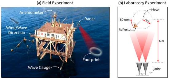
Figure 1.
(a) Aircraft view of the Black sea research platform, (b) Noise estimation experiment.
Simultaneous wave measurements were performed using a resistant wire wave gauge (WG) operated at 20 Hz sampling rate. Wind velocity was measured at 0.2 Hz sampling rate by a vane anemometer installed at 21 m height on platform mast. The anemometer location on the very top of the mast was chosen to avoid wind distortion by platform structures.
We select a typical one hour sample record that includes LF features. The radar was installed at 12 m height at incidence angle and directed upwind (wind and dominant waves both coming from the east). For this observation geometry, the radar surface footprint was about 2 m in width and 4 m in length.
On the measurement day (12 September 2012, Figure 2), the wind speed accelerated at about 04:00 UTC reaching maximum of about 15 m/s by 05:00 UTC. Wave development lagged the wind amplification and then they calmed down after 18:00 UTC. The measurements that we consider were taken between 13:20 UTC and 14:20 UTC when wind waves became steady and no strong swell present. During the acquisition period, the mean wind speed was 6 m/s with 0.7 m significant wave height. The wind wave spectrum (see Section 3.1 below) was close to the saturation level for wave frequency Hz (to within the Toba empirical confidence range [24]) but had a somewhat weaker spectral level between 0.19 Hz and 0.38 Hz. Based on the WG measurements, no surface waves were present below the peak frequency, Hz. Besides somewhat weaker peak spectrum level, the wave state can be considered as a well developed for m/s (wave age ).
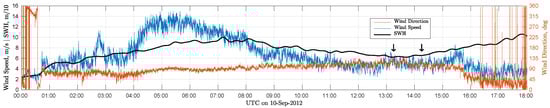
Figure 2.
Wind speed, wind direction, and significant wave height (SWH) on 12 September 2012. Radar acquisition time span is marked by the two black arrows.
2.2. Analyzed Parameters and Their Relations
The instantaneous NRCS, , and DV, , were computed as the 0th and 1st moments of the instantaneous spectrum, , estimated using Fourier transform of raw in-phase and quadrature signals, I/Q, see e.g., [20,25,26] over consecutive s time intervals, ,
where rad/m is the radar wavenumber.
LF variations are visualized by applying the running time mean:
where is the normalized rectangular window with width, s time intervals (approximately two dominant wave periods).
Signal envelope, reflecting group structure, is estimated using the running variance:
The standard relationship between radar signal variations and wave parameters is employed [1,3]. Fourier harmonic, , of DV variations due to orbital velocities of resolved surface waves reads:
where is the Fourier harmonic of wave elevation, is the wave angular frequency, is the geometric coefficient accounting for horizontal and vertical orbital velocity components, is the azimuthal angle between wave vector and radar incidence plane, is the incidence angle. Thus, the Doppler velocity spectrum , and the sea surface elevation spectrum, , are related as
In terms of linear Modulation Transfer Function (MTF), NRCS variation is a linear function of wave slope [1,3]. For upwind radar measurements analyzed in this paper, we suppose that all waves are traveling towards the radar (a unidirectional sea, ). For a single Fourier harmonic, the NRCS response can then be expressed as:
where the overbar, , stands for the time mean, is the NRCS variation, is the Fourier harmonic of wave slope, k is the wavenumber corresponding to , and M is the linear MTF coefficient. To note, is taking into account more rapidly time-space decorrelating processes, including not resolved short scale slope components. Accordingly, represents a relatively slow time and well resolved slope component.
Taking into account the full distribution of these slope components, temporal variations of NRCS then writes:
where is a function of wave frequency.
The MTF can be evaluated from either WG or DV using the deep water gravity wave dispersion relationship, , (applicable to our measurements):
where g is the gravity acceleration, is the NRCS-elevation cross-spectrum, and is the DV-NRCS cross-spectrum.
Conversely, if the MTF is known, the NRCS time series can be reconstructed from either WG or DV given for the presented data. In the frequency range, Hz, the average magnitude of linear MTF is determined from (9) and equals 13.5 and 17 for VV and HH polarization, respectively. The Hilbert transform is applied to DV and WG data to estimate their instantaneous magnitudes and phases. The instantaneous frequency is computed from the instantaneous phase and then averaged over . Equations (5) and (7) are used to retrieve instantaneous wave and radar parameters, z, , v, assuming monochromatic sea within time interval.
2.3. System Noise Estimation
To rule out a possibility that LF variations are instrumental artifacts, the noise introduced by the radar itself was estimated directly. In order to measure the total noise produced by all components of the measuring system, we conducted a test laboratory measurement of a target with time independent properties [27]. The homodyne radar detection system used in this study rejects zero-Doppler (static) targets. The radar was directed on a metal corner reflector spinning at 80 rpm (Figure 1b). The rotation rate was selected so that LF components, Hz, can be captured. The rotation rate stability was achieved by the use of an asynchronous motor powered by a stabilized alternate current source. Note that rotation rate instability can only increase the measured LF DV variations. Hence, this experiment provided an upper limit for the LF DV system noise, while the measured LF NRCS variations are expected to be due to the system noise only. Each time the reflector faced the radar, it produced NRCS and DV signals, from which noise-equivalent spectra , , and were computed.
3. Results
This section presents results of radar field measurements. Observed LF radar spectra are compared with the system noise characteristics. Impact of wind and waves on LF signatures is analyzed based on radar signal comparisons with simultaneous wind and wave measurements. A non-linear modulation transfer function is adopted to explain the observed sample distribution of NRCS as well as its LF variations.
3.1. Observed Low-Frequency Signatures
Measured Ka-band sea surface NRCS and DV (Figure 3) and their corresponding spectra (Figure 4) demonstrate noticeable LF variations similar to those observed by [17,19] in the X-band.
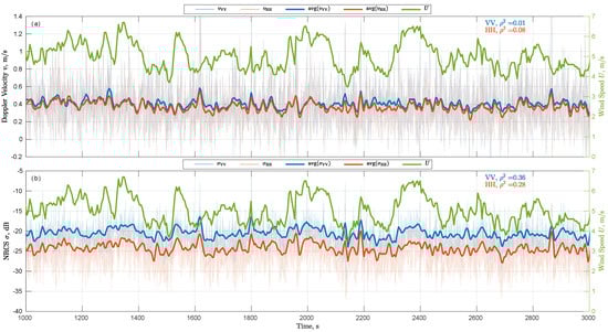
Figure 3.
Time series of 10s-average (top panel) DV and (bottom panel) NRCS. Green–wind speed, bold blue/orange–VV/HH, is the corresponding squared correlation with wind speed.
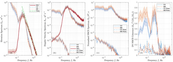
Figure 4.
Spectra of (a) elevations, (b) DV, (c) NRCS, and (d) DV-NRCS coherence function. Dashed lines on (b,c,d) plots correspond to noise equivalent levels. Red–WG measurements, blue/orange–VV/HH polarizations. Green dashed lines correspond to Toba’s, , empirical model [24]. Shading indicates 95% confidence interval. Number of degrees of freedom in spectrum averaging is 35.
Spectral density of DV in the LF range (Figure 4b) is about half of the peak level (HH is slightly higher). Noise spectrum of DV (Figure 4b) is about 4 orders of magnitude weaker and can be neglected. Conversion of DV spectrum to elevation spectrum Equation (6) involves the factor and results in unrealistic spectral behavior in the LF range (Figure 4a).
The LF part of NRCS spectrum is comparable in magnitude to the peak level (Figure 4c) (HH is larger again). The NRCS system noise is also 4 orders of magnitude less than the NRCS signal and is disregarded.
In the LF range, the DV-NRCS coherence (Figure 4d) is non-zero and well above the noise level. The temporal correlation between DV and NRCS is generally positive in LF () and wave () frequency ranges. The total time mean Doppler contribution integrated over the whole frequency domain , contains about 30% relative contribution from the LF part (measured DV-NRCS cross-spectra are shown in Section 3.2 below).
Some of the previous hypotheses of the origin of LF radar variations involve wind turbulence [17]. Comparison of time series of LF DV and NRCS with LF wind speed (Figure 3) suggests that the NRCS is correlated with the wind, while the DV is not. To highlight the impact of wind-induced variations, we estimate NRCS component from which wind-related variations are removed, the wind-removed NRCS hereinafter, , where the wind exponent n is set to 3 and is determined by the linear fit, (Figure 5b). The choice of wind exponent, , is based on the NRCS wind speed dependence [22]. However, varying the wind exponent within does not change results substantially.
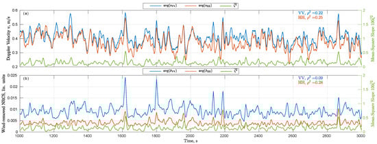
Figure 5.
Time series of (top panel) DV and (bottom panel) wind-removed NRCS, . Green–mean-square slope, bold blue/orange–VV/HH. Average interval is 10 s.
Analysis of the wind-removed NRCS spectra computed with low accuracy but high spectral resolution (5 degrees of freedom) demonstrates that the NRCS is sensitive to the measured wind only for Hz (Figure 6). At higher frequencies, the difference is small suggesting that near surface and anemometer height wind variations are not well correlated. Our wind detection setup was primarily designed to control the background atmospheric conditions, i.e., record-mean wind velocity. The measurement height (21 m) as well as wind vane anemometer sampling rate (0.2 Hz) both are not optimal to detect Hz wind fluctuations, which may be associated with the atmospheric boundary layer perturbations produced by wave groups and confined to lower heights. These high frequency wind perturbations are simply missed by 21-m height sensor. Due to the above wind detection limitations, it might not be.; surprising to see such weak impacts of observed wind fluctuations on NRCS spectra at Hz.
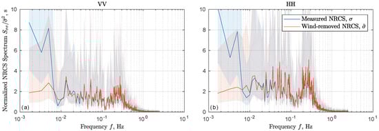
Figure 6.
Measured and wind-removed NRCS spectra for (a) VV and (b) HH polarizations. Shading indicates the 95%-confidence interval.
Alternative mechanisms of the origin of LF radar variations involve wave group structure that modulates (i) surface mean-square slope (MSS), which affects the LF NRCS in accordance with the two-scale model, , where P is the second-order coefficient in the Taylor expansion of in wave slope, [18,28], (ii) intermediate waves to which shorter parasitic waves are bounded (LF DV mechanism [19]), (iii) wave breaking inhomogeneity [21] that imprints on sub-peak frequency variability of both DV and NRCS [20].
As a proxy for wave group, we use the running slope variance, , estimated from radar DV. We compare this “running” MSS with average DV (Figure 5a) and wind-removed NRCS. The LF variations of DV and NRCS are related to the running mean MSS, but to a lesser extent than to the wind speed. As expected from the two-scale model e.g., [18], HH NRCS is more strongly affected by MSS than VV NRCS.
Linear correlation analysis suggests that wind accounts for ∼30% of the total LF NRCS (slower than 10 s) variance, while only 10% (30%) of the residual, non-wind-induced, variance is accounted for by MSS variations at VV (HH) polarization, respectively.
In contrast, LF DV weakly correlates with the wind, however, ∼20% of its variance is explained by MSS variations. Notice that the correlation between DV and MSS is also affected by the fact that the MSS is retrieved from the DV itself (WG data are not used because they were measured far from the radar footprint). DV-based MSS proxy accounts only for waves longer than the radar footprint length that do not respond to immediate wind fluctuations, which in turn explains the rather low correlation between MSS and wind.
3.2. Non-Linear Transfer Function
A non-zero correlation between MSS and LF NRCS reflects a non-linearity of NRCS-wave slope transfer. In general, a non-linear transfer results in spectrum broadening by leaking energy into multiple order harmonics and sub-harmonics [29,30]. Our focus is on the latter as a potential cause of observed LF features in both NRCS and DV.
The impact of non-linearity is demonstrated by the shape of NRCS probability density function (PDF, Figure 7a,b) that is strongly skewed with a well-marked typical heavy-tail distribution. As the linear MTF (7) can be used to interpret the slow-time NRCS modulations from quasi-normally distributed wave slopes, the total retrieved NRCS indeed further compounds this random process to result in a more strongly marked heavy-tail PDF distribution (Figure 7a,b).
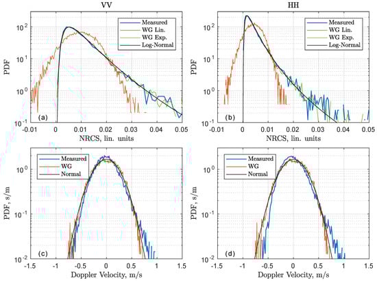
Figure 7.
Probability density function (PDF) of (a,b) NRCS and (c,d) DV for (a,c) VV polarization and (b,d) HH polarization. Blue–measurements, orange–retrieved using linear MTF Equation (7), green–retrieved using non-linear MTF Equation (10), black–theoretical curve (log-normal for NRCS, normal for DV).
Furthermore, as the characteristic magnitude of the linear MTF can be significant (≈10–20), small wave slopes can locally produce NRCS variations comparable in magnitude to the NRCS itself. In line with a two-scale decomposition described as a compound stochastic process, including resolved and non-resolved impact of surface tilts, an alternative non-Linear MTF (NLMTF) can thus be used [31,32,33,34],
to which the traditional linear MTF Equation (7) results from a first order approximation.
For the normally distributed slopes , the NRCS given by Equation (10) is log-normally distributed:
Taking into account this “non-linear” NRCS decomposition, the resulting -parameter is not directly the mean NRCS, , but must take into account a -correction, as:
In line with previous experiments [32], the PDF of observed NRCS is approximated well by a log-normal distribution Equation (11) as shown in Figure 7a,b (MTF magnitude, M, estimated using Equation (9) is used here). Observed NRCS spectra and DV-NRCS cross-spectra are also reproduced well using the NLMTF (Figure 8). As expected, the linear MTF does not produce LF components if applied to WG data. Switching to NLMTF makes LF spectral level non-zero but still lower than in observations. LF components are produced if the DV is used as a wave probe and the linear MTF is applied. Indeed, it reflects the presence of LF components in measured DV. Finally, if DV-based wave elevations are non-linearly transformed into the NRCS, the simulated co- and cross-spectra have well pronounced LF features.
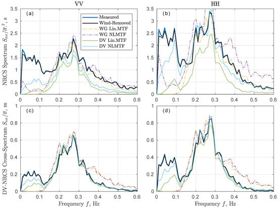
Figure 8.
Measurements and various estimates of (a,b) NRCS spectra and (c,d) real part of DV-NRCS cross-spectra for (a,c) VV polarization and (b,d) HH polarization.
On the other hand, the DV PDF is quasi-Gaussian (Figure 7c,d) indicating that measured DV is reproduced well by WG data using the linear MTF (with the exception of HH polarization for which the PDF is slightly skewed). Hence, LF DV variations cannot directly be explained by the NLMTF. However, the DV measured by a radar is a footprint-averaged local DV, weighted by local NRCS. Because the local NRCS is a non-linear function of local wave slopes, the measured DV is affected by non-linearity of NRCS transfer function. In other words, the observed LF DV signatures can result from both NRCS non-linear modulation and footprint averaging effects.
4. Discussion
This paper suggests that MTF non-linearity is an important factor that explains the observed LF features. Applying the NLMTF to the surface wave elevation reveals a surprising result: the DV-based surface elevation works better than in-situ WG-based surface elevation for radar spectra estimates (Figure 8). This fact may be related to distortions of the apparent frequency of shorter waves by orbital velocity of longer waves, in turn suggesting that WG-based frequency attribution of wave elevation is not reliable at high frequencies. Next, we will perform a numerical simulation to overcome a lack of information on unresolved short waves. The simulation is further used to assess the relative importance of footprint averaging and MTF non-linearity effects.
4.1. Numerical Simulation
To model one-dimensional moving surface, a semi-empirical wavenumber KMC spectrum [35,36] is used. The length of a simulated domain is 400 m (≈10 dominant wavelengths) with a spatial resolution of 0.05 m that corresponds to the shortest simulated surface wavelength of about six Ka-band radar wavelengths. The initial surface is a superposition of waves (Fourier harmonics) with amplitudes obeying the KMC spectrum and phases randomly distributed over interval. The phase speed of each wave is determined by the dispersion relation, , where N/m is the surface tension. All waves propagate towards an upwind looking radar oriented at incidence angle. Simulation duration is 12 hours (about 10000 dominant wave periods) with 0.1 s time step.
Both NRCS and DV are simulated directly omitting I/Q-signal modeling. The local NRCS is computed using NLMTF (10) from simulated surface slopes (local surface gradient), while the local DV is a sum of orbital velocities (5) of all waves.
The radar NRCS and DV are footprint averages:
where is the Gaussian-shaped two-way antenna pattern. We will explore different values of half-width, including 4 m width that corresponds to our radar footprint.
Simulated DV and NRCS spectra, and their cross-spectra are shown in Figure 9 along with measurements. Given a rather simple 1-D surface elevation model, the overall consistency between measurements and simulations is remarkably good. The simulated DV peak level is higher than in observations because all wave energy is directed into a single direction, while the real spectrum is not unidirectional. The simulation nicely reproduces the LF signatures for all spectra with the exception of VV NRCS (Figure 9a). This can be explained by the presence of LF wind variability (not accounted for by this simple 1-D model) to which VV NRCS is more sensitive due to higher contribution of Bragg backscattering. VV cross-spectrum (Figure 9a) is reproduced better than NRCS spectrum, indicating that wind-induced variability is important for NRCS and to a much lesser extent for DV.
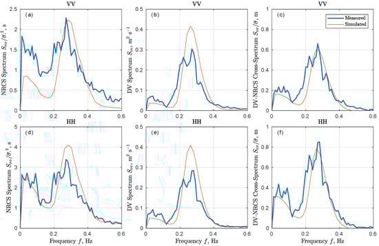
Figure 9.
Simulated and measured (a,d) NRCS, (b,e) DV, (c,f) real part of DV-NRCS cross-spectra for (top row) VV polarization and (bottom row) HH polarization.
Although the hydrodynamics MTF responsible for short-long wave correlation is not directly included in the simulation, its impact on LF variations is partially present through the use of observed MTF magnitude ( 13–17), which otherwise would be lower for the tilting only.
4.2. Footprint Effects
The simulation is used to demonstrate how the LF spectrum is impacted by footprint averaging effects. The DV and NRCS are simulated for different footprint sizes, m, at U = 6 m/s and using the NLMTF Equation (10) with (Figure 10).
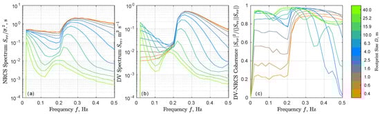
Figure 10.
Simulated spectra of (a) NRCS and (b) DV, and (c) DV-NRCS coherence for various footprint size at m/s and .
The wave peak, Hz, is well pronounced for both NRCS and DV for small D. With increasing D, the high frequencies are attenuated, causing the peak narrowing and shifting towards the LF range. The LF spectrum level is rather flat when D is small, but it intensifies at near zero frequencies with increasing D. The ratio of the spectrum integral in the LF range, , to the spectrum integral in the wind wave frequency range, , increases with increasing D.
The DV-NRCS coherence (Figure 10c) also increases in the LF range with increasing D. For m (corresponding to our observations), the simulated coherence resembles the observed one (Figure 4d) with somewhat lower (but close) values in the LF and wind wave frequency ranges. The coherence peak in the wind wave frequency range narrows with increasing D. For larger m approaching peak wavelength, the shape of coherence complicates, probably reflecting numerical aliasing artifacts.
4.3. Non-Linearity Effects
To evaluate the effect of MTF non-linearity (Figure 11), the footprint is kept constant, m, while M in Equation (10) is varied from 1 to 20. Both NRCS and DV spectra exhibit increasing LF spectral density with increasing MTF magnitude (increasing non-linearity). The growing LF-to-wave-peak ratio for the NRCS (Figure 11a) is expected due to non-linear effects. DV spectrum peak (Figure 11b) does not change with varying M. However, the LF DV spectrum level increases with increasing M, which is explained by a combination of footprint averaging and non-linear modulation.
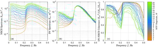
The DV-NRCS coherence (Figure 11c) is similar to observations (Figure 4d). Its LF-to-wave-peak ratio only slightly increases with increasing M, indicating that its behavior is primarily determined by footprint averaging effects rather than MTF non-linearity (Figure 10c).
Finally, we evaluate how good the linear MTF is if the actual transfer function is non-linear. First, the NLMTF, with in Equation (10), is used to simulate DV and NRCS. Then, the linear MTF, with in Equation (9), is inferred from simulated DV and NRCS. Simulations are performed for various NLMTF magnitude, . The footprint size, D, is set to 1 m to increase the footprint cut-off frequency of simulated spectra.
The estimated linear MTF magnitude, , (Figure 12a) equals the original NLMTF magnitude, , for with the upper frequency, , determined by the footprint size. The linear MTF estimate level averaged over Hz frequency interval is close (to within 10% error corridor) to the original NLMTF magnitude for (Figure 12b, blue symbols), although its uncertainty increases at higher .
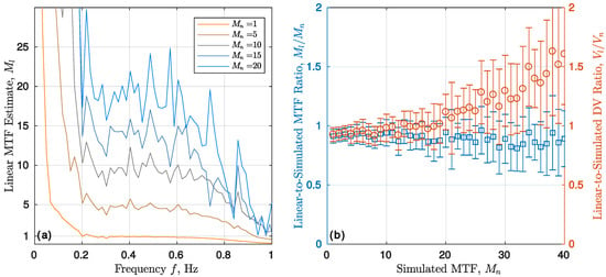
Figure 12.
(a) Linear MTF estimated using Equation (9) for the non-linearly simulated NRCS for various in Equation (10); (b) Left y-axis: ratio of linear MTF estimate, in Equation (9), averaged at Hz Hz to . Right y-axis: ratio of DV estimate based on linear MTF, in Equation (15), to the DV simulated using NLMTF, in Equations (13) and (14).
The time mean DV, or the DV averaged over the whole wave spectrum, is also estimated from linear MTF magnitude, , and known wave spectrum using Equations (5) and (8):
The ratio of DV estimate, , based on linear MTF Equation (15) to the non-linearly simulated DV, , is close to 1 for to within 10% error (Figure 12b). For the majority of practical cases (excluding near-threshold winds and large with > 20 [23]), the impact of non-linear effects on radar DV can be ignored.
One simplification made for DV estimation Equation (15) is the using of frequency independent MTF, which is not the case for a swell that has higher MTF due to wave-induced wind variations [2,37], which are not included in our simple simulations. Thus our numerical simulations suggest that linear MTF Equation (7) is a good approximation for non-linear MTF Equation (10) given small long wave slopes.
5. Conclusions
This study presents the analysis of LF variations of Doppler radar backscattering from the sea surface based on Ka-band field measurements. A specialized laboratory experiment was conducted to estimate the measuring system noise and to prove that it is not the cause of observed LF variations. The LF variations are separated from the signals by applying the running 10-s mean roughly corresponding to double period of dominant waves. LF winds explain about ∼30% of LF NRCS variance, while LF DV does not correlate with LF winds. Non-wind-induced NRCS is partly explained by LF mean-square slope (10%/30% for VV/HH polarization, respectively) indicating non-linear transfer between slopes and NRCS. Note, that 21-m wind correlates with NRCS variations only at frequencies below 0.01 Hz indicating the presence of specific wind near-surface fluctuations (e.g., due to wave groups).
As deducted from the sample distribution analysis, the local NRCS is essentially a non-linear function of wave slopes in line with previous studies [29,30,31,32]. This non-linearity explains observed NRCS spectra, including their LF part, if non-linear MTF is applied to wave slopes estimated from instantaneous radar DV (orbital velocity). The DV has quasi-Gaussian distribution (positive tails are caused by wave breaking), indicating that it is a linear function of surface slopes. Hence, LF variations in radar DV is a consequence of spatial averaging that is a product of the local DV weighted by the local non-linear NRCS.
Impacts of non-linearity and footprint effects are tested using a 1-D surface elevation simulation based on the semi-empirical wave spectrum [35] corresponding to observed wind and wave fetch. If the NRCS is modeled using a non-linear transfer function, the measured DV and NRCS spectra are adequately reproduced by the simulation even though the hydrodynamics effects are not included. Simulated LF variance of VV NRCS is underestimated by a factor of ≈2, suggesting that wind variability, which is not included in the simulation, is still important. However, the DV-NRCS cross-spectrum is simulated well even without the inclusion of wind variability effect. This suggests that LF DV is not strongly affected by LF winds, whose impact can be ignored for the time mean DV.
The relationship between the LF radar signal variation and the non-linearity of modulation transfer function may explain other available observations. In particular, the magnitude of LF variations in the L-band is almost twice as large as in the X-band [17]. This is explained by larger L-band MTF magnitude (e.g., see Figure 11 in [38]) that results in more pronounced non-linearity. The increase of LF level of DV spectra at large incidence angles [19,20] is explained by larger radar footprint size and by larger MTF magnitude caused by hydrodynamics modulation of wedge scattering.
Simulations with different footprint sizes and MTF magnitudes show that MTF non-linearity has little effect on estimated linear MTF as well as on estimated time mean DV. This confirms that traditional linear MTF [1,3] is a good approximation for real non-linear radar MTF, while LF signatures are “artifacts” caused by MTF non-linearity and/or spatial averaging over finite radar footprint.
Author Contributions
V.N.K. and Y.Y.Y. conceived and designed the experiments; V.N.K., B.C. and S.A.G. provided sea surface model for numerical simulations; Y.Y.Y. performed the experiments, analyzed the data, and wrote the paper.
Acknowledgments
The core support of the work was provided by Russian Science Foundation grant No. 17-77-10052. Field experiments were supported by the FASO of Russia under the State Assignment (No. 0827-2018-0002). Sea surface simulation was supported by the Ministry of Science and Education (Goszadanie 5.2928.2017/PP) and NASA/PhO. The authors would like to thank Anton Garmashov of MHI for providing meteorological measurements.
Conflicts of Interest
The authors declare no conflict of interest.
Abbreviations
The following abbreviations are used in this manuscript:
| DV | Doppler Velocity |
| FFT | Fast Fourier Transform |
| HH | Horizontal Transmit-Receive Polarization |
| LF | Low Frequency |
| MSS | Mean-Square Slope |
| MTF | Modulation Transfer Function |
| NLMTF | Non-Linear Modulation Transfer Function |
| NRCS | Normalized Radar Cross-Section |
| Probability Density Function | |
| VV | Vertical Transmit-Receive Polarization |
| UTC | Coordinated Universal Time |
| WG | Wave Gauge |
References
- Keller, W.C.; Wright, J.W. Microwave scattering and the straining of wind-generated waves. Radio Sci. 1975, 10, 139–147. [Google Scholar] [CrossRef]
- Schröter, J.; Feindt, F.; Alpers, W.; Keller, W.C. Measurement of the ocean wave-radar modulation transfer function at 4.3 GHz. J. Geophys. Res. (Oceans) 1986, 91, 923–932. [Google Scholar] [CrossRef]
- Plant, W.J. The Modulation Transfer Function: Concept and Applications. In Radar Scattering from Modulated Wind Waves; Springer: Berlin, Germany, 1989; pp. 155–172. [Google Scholar]
- Goldstein, R.M.; Zebker, H.A. Interferometric radar measurement of ocean surface currents. Nature 1987, 328, 707–709. [Google Scholar] [CrossRef]
- Romeiser, R.; Thompson, D.R. Numerical study on the along-track interferometric radar imaging mechanism of oceanic surface currents. IEEE Trans. Geosci. Remote Sens. 2000, 38, 446–458. [Google Scholar] [CrossRef]
- Martin, A.; Gommenginger, C. Towards wide-swath high-resolution mapping of total ocean surface current vectors from space: Airborne proof-of-concept and validation. Remote Sens. Environ. 2017, 197, 58–71. [Google Scholar] [CrossRef]
- Chapron, B.; Collard, F.; Ardhuin, F. Direct measurements of ocean surface velocity from space: Interpretation and validation. J. Geophys. Res. (Oceans) 2005, 110, 7008. [Google Scholar] [CrossRef]
- Johannessen, J.A.; Chapron, B.; Collard, F.; Kudryavtsev, V.; Mouche, A.; Akimov, D.; Dagestad, K.F. Direct ocean surface velocity measurements from space: Improved quantitative interpretation of Envisat ASAR observations. Geophys. Res. Lett. 2008, 35, 22608. [Google Scholar] [CrossRef]
- Mouche, A.A.; Collard, F.; Chapron, B.; Dagestad, K.F.; Guitton, G.; Johannessen, J.A.; Kerbaol, V.; Hansen, M.W. On the Use of Doppler Shift for Sea Surface Wind Retrieval From SAR. IEEE Trans. Geosci. Remote Sens. 2012, 50, 2901–2909. [Google Scholar] [CrossRef]
- Bourassa, M.A.; Rodriguez, E.; Chelton, D. Winds and currents mission: Ability to observe mesoscale AIR/SEA coupling. Proc. Int. Geosci. Remote Sens. Symp. 2016, 7392–7395. [Google Scholar] [CrossRef]
- Ardhuin, F.; Aksenov, Y.; Benetazzo, A.; Bertino, L.; Brandt, P.; Caubet, E.; Chapron, B.; Collard, F.; Cravatte, S.; Dias, F.; et al. Measuring currents, ice drift, and waves from space: the Sea Surface KInematics Multiscale monitoring (SKIM) concept. Ocean Sci. Discuss. 2017, 2017, 1–26. [Google Scholar] [CrossRef]
- Bao, Q.; Lin, M.; Zhang, Y.; Dong, X.; Lang, S.; Gong, P. Ocean Surface Current Inversion Method for a Doppler Scatterometer. IEEE Trans. Geosci. Remote Sens. 2017, 55, 6505–6516. [Google Scholar] [CrossRef]
- Rodriguez, E.; Wineteer, A.; Perkovic-Martin, D.; Gál, T.; Stiles, B.; Niamsuwan, N.; Rodriguez Monje, R. Estimating Ocean Vector Winds and Currents Using a Ka-Band Pencil-Beam Doppler Scatterometer. Remote Sens. 2018, 10, 576. [Google Scholar] [CrossRef]
- Nouguier, F.; Chapron, B.; Collard, F.; Mouche, A.; Rascle, N.; Ardhuin, F.; Wu, X. Sea Surface Kinematics From Near-Nadir Radar Measurement. IEEE Trans. Geosci. Remote Sens. 2018. accepted. [Google Scholar]
- Fois, F.; Hoogeboom, P.; Le Chevalier, F.; Stoffelen, A. An analytical model for the description of the full-polarimetric sea surface Doppler signature. J. Geophys. Res. (Oceans) 2015, 120, 988–1015. [Google Scholar] [CrossRef]
- Yurovsky, Y.Y.; Grodsky, S.A.; Kudryavtsev, V.N.; Chapron, B. Wave-induced Doppler shift of Ka-band radar signal backscattered from the sea surface. In Proceedings of the 2017 Progress in Electromagnetics Research Symposium-Fall (PIERS-FALL), Singapore, 19–22 November 2017; pp. 2299–2306. [Google Scholar]
- Plant, W.J.; Keller, W.C.; Cross, A. Parametric dependence of ocean wave-radar modulation transfer functions. J. Geophys. Res. (Oceans) 1983, 88, 9747–9756. [Google Scholar] [CrossRef]
- Grodsky, S.A.; Kudryavtsev, V.N.; Bol’shakov, A.N.; Smolov, V.E. Experimental investigation of fluctuations of radar signals caused by surface waves. Phys. Ocean. 2001, 11, 333–352. [Google Scholar] [CrossRef]
- Plant, W.J. A model for microwave Doppler sea return at high incidence angles: Bragg scattering from bound, tilted waves. J. Geophys. Res. (Oceans) 1997, 102, 21131–21146. [Google Scholar] [CrossRef]
- Hwang, P.A.; Sletten, M.A.; Toporkov, J.V. A note on Doppler processing of coherent radar backscatter from the water surface: With application to ocean surface wave measurements. J. Geophys. Res. (Oceans) 2010, 115, C03026. [Google Scholar] [CrossRef]
- Donelan, M.; Longuet-Higgins, M.S.; Turner, J.S. Periodicity in whitecaps. Nature 1972, 239, 449–451. [Google Scholar] [CrossRef]
- Yurovsky, Y.Y.; Kudryavtsev, V.N.; Grodsky, S.A.; Chapron, B. Ka-Band Dual Copolarized Empirical Model for the Sea Surface Radar Cross Section. IEEE Trans. Geosci. Remote Sens. 2017, 55, 1629–1647. [Google Scholar] [CrossRef]
- Yurovsky, Y.Y.; Kudryavtsev, V.N.; Chapron, B.; Grodsky, S.A. Modulation of Ka-band Doppler Radar Signals Backscattered from the Sea Surface. IEEE Trans. Geosci. Remote Sens. 2018, 1–19. [Google Scholar] [CrossRef]
- Toba, Y.; Koga, M. A parameter describing overall conditions of wave breaking, whitecapping, sea-spray production and wind stress. In Oceanic Whitecaps; Monahan, E.C., Niocaill, G.M., Eds.; Reidel Publishing Company: Boston, MA, USA, 1986; pp. 37–47. [Google Scholar]
- Jessup, A.T.; Melville, W.K.; Keller, W.C. Breaking waves affecting microwave backscatter 1. Detection and verification. J. Geophys. Res. (Oceans) 1991, 96, 20547–20559. [Google Scholar] [CrossRef]
- Thompson, D.R.; Jensen, J.R. Synthetic aperture radar interferometry applied to ship-generated internal waves in the 1989 Loch Linnhe experiment. J. Geophys. Res. (Oceans) 1993, 98, 10259–10270. [Google Scholar] [CrossRef]
- Klugmann, D.; Stephan, R. Calibration of portable FM-CW Doppler radar profilers with an artificial target. Proc. Int. Geosci. Remote Sens. Symp. 2004, 6, 3953–3955. [Google Scholar] [CrossRef]
- Kudryavtsev, V.; Hauser, D.; Caudal, G.; Chapron, B. A semiempirical model of the normalized radar cross-section of the sea surface 1. Background model. J. Geophys. Res. (Oceans) 2003, 108, C08054. [Google Scholar] [CrossRef]
- Hesany, V.; Moore, R.K.; Gogineni, S.P.; Holtzman, J.C. Slope-induced nonlinearities on imaging of ocean waves. IEEE J. Oceanic Eng. 1991, 16, 279–284. [Google Scholar] [CrossRef]
- Schmidt, A.; Bao, M. The modulation of radar backscatter by long ocean waves: A quadratically nonlinear process? J. Geophys. Res. (Oceans) 1998, 103, 5551–5562. [Google Scholar] [CrossRef]
- Trunk, G.V. Radar Properties of Non-Rayleigh Sea Clutter. IEEE Trans. Aerosp. Electron. Syst. 1972, AES-8, 196–204. [Google Scholar] [CrossRef]
- Gotwols, B.L.; Thompson, D.R. Ocean microwave backscatter distributions. J. Geophys. Res. (Oceans) 1994, 99, 9741–9750. [Google Scholar] [CrossRef]
- Thompson, D.R.; Gotwols, B.L. Comparisons of model predictions for radar backscatter amplitude probability density functions with measurements from SAXON. J. Geophys. Res. (Oceans) 1994, 99, 9725–9739. [Google Scholar] [CrossRef]
- Nouguier, F.; Guerin, C.A.; Chapron, B. Scattering From Nonlinear Gravity Waves: The “Choppy Wave” Model. IEEE Trans. Geosci. Remote Sens. 2010, 48, 4184–4192. [Google Scholar] [CrossRef]
- Kudryavtsev, V.N.; Makin, V.K.; Chapron, B. Coupled sea surface-atmosphere model: 2. Spectrum of short wind waves. J. Geophys. Res. (Oceans) 1999, 104, 7625–7639. [Google Scholar] [CrossRef]
- Yurovskaya, M.V.; Dulov, V.A.; Chapron, B.; Kudryavtsev, V.N. Directional short wind wave spectra derived from the sea surface photography. J. Geophys. Res. (Oceans) 2013, 118, 4380–4394. [Google Scholar] [CrossRef]
- Alpers, W.; Ross, D.; Rufenach, C. On the detectability of ocean surface waves by real and synthetic aperture radar. J. Geophys. Res. (Oceans) 1981, 86, 6481–6498. [Google Scholar] [CrossRef]
- Feindt, F.; Schroeter, J.; Alpers, W. Measurement of the ocean wave-radar modulation transfer function at 35 GHz from a sea-based platform in the North Sea. J. Geophys. Res. (Oceans) 1986, 91, 9701–9708. [Google Scholar] [CrossRef]
© 2018 by the authors. Licensee MDPI, Basel, Switzerland. This article is an open access article distributed under the terms and conditions of the Creative Commons Attribution (CC BY) license (http://creativecommons.org/licenses/by/4.0/).