The Generalized Gamma-DBN for High-Resolution SAR Image Classification

Abstract

With the increase of resolution, effective characterization of synthetic aperture radar (SAR) image becomes one of the most critical problems in many earth observation applications. Inspired by deep learning and probability mixture models, a generalized Gamma deep belief network (g$\mathsf{\Gamma }$-DBN) is proposed for SAR image statistical modeling and land-cover classification in this work. Specifically, a generalized Gamma-Bernoulli restricted Boltzmann machine (g$\mathsf{\Gamma }$B-RBM) is proposed to capture high-order statistical characterizes from SAR images after introducing the generalized Gamma distribution. After stacking the g$\mathsf{\Gamma }$B-RBM and several standard binary RBMs in a hierarchical manner, a g$\mathsf{\Gamma }$-DBN is constructed to learn high-level representation of different SAR land-covers. Finally, a discriminative neural network is constructed by adding an additional predict layer for different land-covers over the constructed deep structure. Performance of the proposed approach is evaluated via several experiments on some high-resolution SAR image patch sets and two large-scale scenes which are captured by ALOS PALSAR-2 and COSMO-SkyMed satellites respectively.

1. Introduction

As a result of its all-weather and timeless imaging capacity, the synthetic aperture radar (SAR) has become one of the most critical techniques in earth observation, such as land cover and crop classification [1], disaster evaluation [2], urban extraction [3] and so on. With the increasing number of SAR sensors, many images are produced in high-quality to provide precise information on the observed land covers. To obtain a solid comprehension of SAR images, one of the most critical problems is how to effectively distinguish different land-covers. A variety of approaches has been proposed to characterize SAR images in recent years, including backscattering coefficients [4], statistical features [5,6], texture descriptors [7], bag-of-words [8], sparse representation [9] and so on. However, the backscattering coefficients heavily depend on imaging parameters, such as electromagnetic properties, frequency, polarization mode, atmospheric condition, soil moisture and so on. It is difficult to apply these features on SAR images which are captured by different sensors. Besides, the increased resolution makes spatial structure of SAR images even heterogeneous, because many tiny objects could be observed clearly in a single resolution cell. Therefore, much more efficient statistical distributions should be developed to characterize such a complex scene.

Compared with SAR images in median or low resolutions, a higher resolution implies that a reduced number of scatters was observed in a single resolution cell. Therefore, a variety of backscatters from distinct land-covers could be received in a single high resolution SAR scene. In recent years, many probability mixture models were proposed to characterize the generative procedure a high-resolution SAR images. In [10], a dictionary-based approach was proposed to model the probability density of SAR image amplitude, in which each component of the dictionary is constructed from some specific probability distributions. However, the likelihood function of MoLC is not guaranteed to be monotonically increasing. Combing both amplitude and texture statistics, a non-stationary Multinomial Logistic latent class label model [11] is proposed to obtain spatial smoothness class segments, which is a mixture of Nakagmi distribution and t-distribution for amplitude and texture respectively. Besides, several mixture distributions, such as mixture of Cauchy-Rayleigh distribution [12], mixture of generalized Gamma [5] and mixture of Wishart distribution [13], are also proposed to characterize and distinct different land-covers. Nevertheless, it is confusing to determine an adaptive number of mixture components for various land-covers. At the same times, the expectation-maximization procedure for parameter optimization is time-consuming.

With developments of machine learning techniques, deep learning, especially the convolutional neural network (CNN), has attracted much attention of many researchers [14,15]. It attempts to create a hierarchical structure by learning simple concepts first and then successfully building more complex concepts. Zhang et al. [16] and Zhu et al. [17] review the latest developments on Deep learning techniques for remote sensing data processing. Because of their high-level semantic feature learning capacity, all of these surveys confirm the excellent performance of deep learning based approaches in remote sensing data analysis. For SAR images, a deep convolutional autoencoder [18] is proposed to extract features and conduct classification automatically by combing several convolutional layer, scalar transformation layer and sparse autoencoders together. At the same time, to reduce overfitting caused by the limited training samples when applying deep CNN for SAR target classification, an all-convolutional networks [19] is proposed by replacing the fully connected layer in the CNN with a sparsely connected layer. By leveraging knowledge learned from sufficient unlabeled SAR scene images, a transfer learning based CNN model [20] is proposed for SAR image target classification with limited labeled data. After exploiting CNN and multi-layer perceptron [21], a deep neural network is proposed to classify different land-covers with the learned high-level features which encode both the spectral and spatial information of pixels in remote sensing images. In addition, many techniques were utilized to improve the classification accuracy of the proposed deep network, such as leveraging a synthetic target database for data augmentation [22], complex-valued domain extension [23] and so on. Besides, several tensor-based CNN approaches [24,25] are proposed for remote sensing image processing. Because they can organize better weights of deep learning structure, these methods reduce the computational complexity of network training and retain the spatial structure of remote sensing images effectively. However, some of tensor-based approaches [26] may over-smooth part of line-type and point-type targets, such as boulevards and bridges, due to the fact that the patches charactering of these pixels. All of these works report a better classification or recognition accuracies due to the fact that deep networks can extract effective features compared with the other methods. As the depth of CNN becoming deeper and deeper, it requires large-scale dataset massive computing power for model training, which is hard to reach in SAR image processing and understanding tasks.

To model the generative procedure of SAR image directly, the deep belief network (DBN) [27,28] is also utilized widely to learn the statistical characterizes of SAR images and used to distinct different land-covers. Specifically, the DBN can be treated as a multi-layer generative graph model, in which each layer is made of a restricted Boltzmann machine (RBM) [29]. The RBM is an undirected, generative energy based graph model with an input layer and a hidden layer, in which the statistical dependencies among each unit in the input layer are encoded in hidden layer. Several constraints DBNs with $l_1$, $l_2$ and $l_{1/2}$ [30] were proposed to build a hierarchical structure for SAR image automatic target recognition. Besides, a Wishart-DBN [31] is proposed to classify different land-covers by employing the prior knowledge of polarimetric SAR images. To release the inadequate effect of data volume, an RBM [32] based adaptive boosting model is proposed for object-oriented classification of polarimetric SAR imagery. Meanwhile, a discriminant deep belief network [33] is proposed to learning high-level features for SAR images classification, in which the discriminant informations are captured by combing ensemble learning with a deep belief network in an unsupervised manner.

Inspired by the work of Nair et al. [34], a generalized Gamma deep belief network (g$\mathsf{\Gamma }$-DBN) is proposed in this work to model the statistical characterizes of high-resolution SAR images. Specifically, the major contributes of this paper are listed as follows.

• A generalized Gamma-Bernoulli RBM (g$\mathsf{\Gamma }$B-RBM) is proposed to learn the statistical model of high-resolution SAR images after casting it as a particular probability mixture model of the generalized Gamma distributions.
• By stacking the g$\mathsf{\Gamma }$B-RBM and several standard binary restricted Boltzmann machines, a generalized Gamma DBN (g$\mathsf{\Gamma }$-DBN) is constructed to learn high-level representations of different land-covers.

Experimental results demonstrate that the proposed approach has excellent capacity of high-resolution SAR image statistical modeling and land-cover classification.

The remainder of this paper is organized as follows. In Section 2, details of the proposed approach are presented. In Section 3, we show quantitative results of our approach after comparing to the other state-of-art approaches. Finally, some conclusions and future works are presented in the last section.

2. Materials and Methods

Because the DBN can be used to learn the statistical dependencies among each units of the observed variables, a generalized Gamma distribution based DBN is proposed in the following section for high-resolution SAR images. By stacking the RBMs in a hierarchical manner, a g$\mathsf{\Gamma }$-DBN is proposed to learn the discriminative information from high-resolution SAR images.

2.1. g$\mathsf{\Gamma }$B-RBM

As a basic structure of DBN, the RBM is a parametrized model which is utilized to represent some probability distributions. It can be employed to learn some important aspects of an unknown target distribution based on some available samples [35]. Typically, the RBM could be viewed as a Markov random field (MRF) associated with a bipartite undirected graph to model the joint distribution of input and output variables. To characterize SAR images in higher resolutions, the generalized Gamma distribution (g$\mathsf{\Gamma }$D) [36,37] is utilized widely to model different land-covers since it has been proposed. Formally, the g$\mathsf{\Gamma }$D is defined as:

$$p\left(x\right)=\frac{\beta }{\sigma \mathsf{\Gamma }\left(\alpha \right)}{\left(\frac{x}{\sigma }\right)}^{\alpha \beta -1}exp\left(-{\left(\frac{x}{\sigma }\right)}^{\beta }\right),\mathrm{where}x\in {\mathbb{R}}^{+}$$

(1)

where $\beta >0$, $\alpha >0$ and $\sigma >0$ are power, shape and scale of g$\mathsf{\Gamma }$D. $\mathsf{\Gamma }\left(\alpha \right)$ is a Gamma function, which is computed by $\mathsf{\Gamma }\left(\alpha \right)={\int }_0^{+\infty }{x}^{\alpha -1}{e}^{-x}\mathrm{d}x$. Several probability distributions which are widely used for SAR statistical modeling can be viewed as a special case of g$\mathsf{\Gamma }$D with different parameters, such as exponential, Rayleigh, Weibull and Gamma distributions. Specifically, some probability density functions of g$\mathsf{\Gamma }$D with different parameter settings are plotted in Figure 1.

After introducing g$\mathsf{\Gamma }$D, a g$\mathsf{\Gamma }$B-RBM is constructed to learn the statistical characterizes of high-resolution SAR images. Specifically, it consists of m visible units $\mathbf{v}=\left(v_1,v_2,\dots ,v_m\right)\in {\left[0,1\right]}^m$ and n hidden units $\mathbf{h}=\left(h_1,h_2,\dots ,h_n\right)\in {\left\{0,1\right\}}^n$. In g$\mathsf{\Gamma }$B-RBM, visible units represent the observed variables which are employed as input. Meanwhile, hidden units are utilized to model statistical relations between observed variables, which is the output of g$\mathsf{\Gamma }$B-RBM.

Following the Gibbs distribution, the joint probability of g$\mathsf{\Gamma }$B-RBM can be given by:

$$p\left(\mathbf{v},\mathbf{h};\theta \right)=\frac{1}{\mathcal{Z}\left(\theta \right)}exp\left(-E\left(\mathbf{v},\mathbf{h};\theta \right)\right)$$

(2)

where $E\left(\mathbf{v},\mathbf{h};\theta \right)$ is the energy function and $\theta$ is the model parameter. The normalized factor $\mathcal{Z}\left(\theta \right)$ can be computed as $\mathcal{Z}\left(\theta \right)={\sum }_{\mathbf{h},\mathbf{v}}exp\left(-E\left(\mathbf{v},\mathbf{h};\theta \right)\right)$, which is also called as partition function.

In this work, the energy function of g$\mathsf{\Gamma }$B-RBM can be defined as:

$$E\left(\mathbf{v},\mathbf{h};\theta \right)=-\sum _{i=1}^n\sum _{j=1}^m{W}_{ij}{h}_i\left(ln{v}_j\right)-\sum _{j=1}^m\left(v_j^{\beta }-b_{j}ln{v}_j\right)-\sum _{i=1}^n{c}_i{h}_i$$

(3)

with model parameter $\theta =\left\{\mathbf{W},\mathbf{b},\mathbf{c}\right\}$. $\mathbf{W}$ is a matrix of weights, i.e., $\mathbf{W}=\left(W_{ij}\right)$, in which each element $W_{ij}$ is a real-valued weight associated with edge between visible unit $v_j$ and hidden unit $h_i$ for $i\in \left\{1,2,\dots ,n\right\}$ and $j\in \left\{1,2,\dots ,m\right\}$. $\mathbf{b}=\left(b_j\right)$ and $\mathbf{c}=\left(c_i\right)$ are bias vectors, in which element $b_j$ and $c_i$ are associated with the jth visible and the ith hidden units respectively. Furthermore, $\beta$ is the power of g$\mathsf{\Gamma }$D.

With energy function declared in Equation (3), the marginal distribution over visible units $\mathbf{v}$ takes the form:

$$\begin{array}{cc}\hfill p\left(\mathbf{v};\theta \right)& =\sum _{\mathbf{h}}p\left(\mathbf{v},\mathbf{h};\theta \right)\hfill \\ \hfill & =\frac{1}{Z\left(\theta \right)}\sum _{\mathbf{h}}exp\left(-E\left(\mathbf{v},\mathbf{h};\theta \right)\right)\hfill \\ \hfill & =\frac{1}{\mathcal{Z}\left(\theta \right)}\prod _{j=1}^m{v}_j^{b_j}exp\left(-v_j^{\beta }\right)\prod _{i=1}^n\left(1+exp\left(c_i+\sum _{j=1}^m{W}_{ij}\left(ln{v}_j\right)\right)\right)\hfill \end{array}$$

(4)

where $\mathcal{Z}\left(\theta \right)={\sum }_{\mathbf{h}}\int p\left({\mathbf{v}}^{\prime },\mathbf{h};\theta \right)\mathrm{d}{\mathbf{v}}^{\prime }$ is the normalized factor. It indicates that g$\mathsf{\Gamma }$B-RBM can also be interpreted as a product of experts [38], in which it combines multiple latent-variable models of the same observation data by multiplying their probability and re-normalizing. Specifically, the partition function of g$\mathsf{\Gamma }$B-RBM can be computed by:

$$\mathcal{Z}\left(\theta \right)=\sum _{\mathbf{h}}exp\left(\sum _{i=1}^n{c}_i{h}_i\right)\prod _{j=1}^m\left(\sum _{i=1}^n{W}_{ij}{h}_i+b_j\right)\int \left(v_{j}exp\left(-v_j^{\beta }\right)\right)\mathrm{d}{v}_j.$$

(5)

In order to simplify the presentation, the calculation procedures of Equations (4) and (5) are listed in Appendix A.

Then, the conditional probability of g$\mathsf{\Gamma }$B-RBM can be given by:

$$\begin{array}{cc}p\left(v_j=x|h ;\theta \right)\hfill & =\frac{p\left(v_j=x,h ;\theta \right)}{p\left(h ;\theta \right)}\hfill \\ \hfill & \propto \exp \left(-E\left(v_j=x,h ;\theta \right)\right)\hfill \\ \hfill & =\exp (\left(b_j\right)\mathrm{In}x-x^{\beta }+{\displaystyle \sum }_{i=1}^n{W}_{ij}{h}_i\left(\mathrm{In} x\right)\hfill \\ \hfill & =x^{\alpha }\exp \left(-x^{\beta }\right)\hfill \end{array}$$

(6)

$$\begin{array}{cc}\hfill p\left(h_i=1\left|\mathbf{v}\right.;\theta \right)& =\mathrm{sig}\left(\sum _{j=1}^m{W}_{ij}\left(ln{v}_j\right)+c_i\right)\hfill \end{array}$$

(7)

where $\alpha =b_j+{\sum }_{i=1}^n{W}_{ij}{h}_i$. $\mathrm{sig}\left(x\right)$ is the logistic function defined as $\mathrm{sig}\left(x\right)={\left(1+exp\left(-x\right)\right)}^{-1}$. Therefore, the probability that g$\mathsf{\Gamma }$B-RBM assigns to a training SAR image sample raised by adjusting the weights $\mathbf{W}$ and biases $\mathbf{b}$, $\mathbf{c}$ to lower the energy of that image and to raise the energy of the other samples.

Similar to MRF, the g$\mathsf{\Gamma }$B-RBM can be learned by approximating the gradient of the log probability of the training SAS samples [38]. With model parameter $\theta$, the log-likelihood can be denoted as:

$$\mathcal{L}\left(\theta \left|\mathbf{v}\right.\right)=p\left(\mathbf{v};\theta \right).$$

Then, the derivative of the log-likelihood with respect to model parameter $\theta$ could be obtained directly from Equation (8) as (details are listed in Appendix B):

$$\frac{\partial ln\mathcal{L}\left(\theta \left|\mathbf{v}\right.\right)}{\partial \theta }=-\sum _{\mathbf{h}}p\left(\mathbf{h}\left|\mathbf{v}\right.;\theta \right)\frac{\partial E\left(\mathbf{v},\mathbf{h};\theta \right)}{\partial \theta }+\sum _{\mathbf{h}}p\left(\mathbf{h}\left|\mathbf{v}\right.;\theta \right)\int p\left(\mathbf{v}\right)\mathrm{d}\mathbf{v}\frac{\partial E\left(\mathbf{v},\mathbf{h};\theta \right)}{\partial \theta }$$

(8)

where

$$\frac{\partial E\left(\mathbf{v},\mathbf{h};W_{ij}\right)}{\partial W_{ij}}=h_{i}ln{v}_j,\frac{\partial E\left(\mathbf{v},\mathbf{h};W_{ij}\right)}{\partial b_j}=ln{v}_j,\frac{\partial E\left(\mathbf{v},\mathbf{h};W_{ij}\right)}{\partial c_i}=h_i.$$

(9)

In this work, a pre-determined value of $\beta$ is utilized in experiments instead of a learning one.

Given a set of training SAR samples, i.e., $\mathcal{V}={\left\{{\mathbf{v}}_p\right\}}_{p=1}^P$, the mean of derivation in Equation (8) becomes:

$$\frac{1}{P}\sum _{\mathbf{v}\in \mathcal{V}}\frac{\partial ln\mathcal{L}\left(\theta \left|\mathbf{v}\right.\right)}{\partial \theta }={\mathbb{E}}_{\mathrm{data}}\left[\frac{\partial E\left(\mathbf{v},\mathbf{h};\theta \right)}{\partial \theta }\right]-{\mathbb{E}}_{\mathrm{model}}\left[\frac{\partial E\left(\mathbf{v},\mathbf{h};\theta \right)}{\partial \theta }\right]$$

(10)

where ${\mathbb{E}}_{\mathrm{data}}\left[·\right]$ is expectation with respect to data, and ${\mathbb{E}}_{\mathrm{model}}\left[·\right]$ is the expectation with respect to the distribution defined by the energy of g$\mathsf{\Gamma }$B-RBM (Equation (3)).

To approximate the gradient of log-likelihood, a K-step contrastive divergence (K-CD) algorithm [35,38] is also applied in this work. Specifically, a Gibbs chain [39] is carried out for only K steps to approximating the expectation ${\mathbb{E}}_{\mathrm{model}}\left[·\right]$, instead of sampling from the RBM-distribution (in Equation (10)) directly. It is initialized by the training SAR image samples ${\mathbf{v}}^{\left(0\right)}$ and yields the sample ${\mathbf{v}}^{\left(K\right)}$ after K steps. Two sampling procedures are carried out in each step, which are firstly sampling ${\mathbf{h}}^{\left(k\right)}$ from $p\left(\mathbf{h}\left|{\mathbf{v}}^{\left(k\right)}\right.\right)$ and followed by sampling ${\mathbf{v}}^{\left(k+1\right)}$ from $p\left(\mathbf{v}\left|{\mathbf{h}}^{\left(k\right)}\right.\right)$. For SAR image sample ${\mathbf{v}}^{\left(0\right)}$, the derivative in Equation (8) could be approximated by:

$$G_K\left({\mathbf{v}}^{\left(0\right)};\theta \right)=-\sum _{\mathbf{h}}p\left(\mathbf{h}\left|{\mathbf{v}}^{\left(0\right)}\right.;\theta \right)\frac{\partial E\left({\mathbf{v}}^{\left(0\right)},\mathbf{h};\theta \right)}{\partial \theta }+\sum _{\mathbf{h}}p\left(\mathbf{h}\left|{\mathbf{v}}^{\left(K\right)}\right.;\theta \right)\frac{\partial E\left({\mathbf{v}}^{\left(K\right)},\mathbf{h};\theta \right)}{\partial \theta }.$$

(11)

The derivative of each component in $\theta$ can be obtained by substituting Equation (8) into Equation (10) respectively. Similar to the work of Fischer et al. [35], a batch-wise K-CD algorithm for g$\mathsf{\Gamma }$B-RBM training is implemented in Algorithm 1.

Algorithm 1K-CD for g$\mathsf{\Gamma }$B-RBM update for a mini-batch of size $N_S$
Input: A g$\mathsf{\Gamma }$B-RBM with m visual units and n hidden units and training batch S.
Output: The gradient approximation of model parameter: $\Delta W_{ij}$, $\Delta b_j$ and $\Delta c_i$, for $i=1,\dots ,n$ and $j=1,\dots ,m$.
1:	Initialization: $\Delta W_{ij}=0$, $\Delta b_j=0$ and $\Delta c_i=0$;
2:	for all $\mathbf{v}\in S$ do
3:	${\mathbf{v}}^{\left(0\right)}\leftarrow \mathbf{v}$;
4:	for $k=1$ to $K-1$ do
5:	$\forall i\in \left\{1,2,\dots ,n\right\}$, sample $h_i^{\left(k\right)}\sim p\left(h_i\left|{\mathbf{v}}^{\left(k\right)}\right.\right)$;
6:	$\forall j\in \left\{1,2,\dots ,m\right\}$, sample $v_i^{\left(k+1\right)}\sim p\left(v_j\left|{\mathbf{h}}^{\left(k\right)}\right.\right)$;
7:	end for
8:	for $1\le i\le n$ and $1\le j\le m$ do
9:	Update $\Delta W_{ij}$: $\Delta W_{ij}\leftarrow \Delta W_{ij}+p\left(\left.h_i=1\right|{\mathbf{v}}^{\left(0\right)}\right)·ln{v}_j^{\left(0\right)}-p\left(\left.h_i=1\right|{\mathbf{v}}^{\left(K\right)}\right)·ln{v}_j^{\left(K\right)}$;
10:	Update $\Delta b_j$: $\Delta b_j\leftarrow \Delta b_j+ln{v}_j^{\left(0\right)}-ln{v}_j^{\left(K\right)}$;
11:	Update $\Delta c_i$: $\Delta c_i\leftarrow \Delta c_i+p\left(\left.h_i=1\right|{\mathbf{v}}^{\left(0\right)}\right)-p\left(\left.h_i=1\right|{\mathbf{v}}^{\left(K\right)}\right)$;
12:	end for
13:	end for
14:	return$\Delta W_{ij}$, $\Delta b_j$ and $\Delta c_i$.

In Algorithm 1, gradients of each parameter are initialized as zeros in step 1 firstly. Then, for all of the SAR image samples in the training batch S, two sampling procedures are carried out sequentially. For each hidden units, it is sampled in step 5 following the condition distribution $p\left(h_i\left|{\mathbf{v}}^{\left(k\right)}\right.\right)$. Meanwhile, each visual unit is sampled following the condition distribution $p\left(v_j\left|{\mathbf{h}}^{\left(k\right)}\right.\right)$ in step 6. Finally, the gradient of each parameter is updated in step 9 to step 11 respectively. Similar to the work of Upadhya et al. [40], let us suppose the computational cost of one Gibbs sampling epoch is T and that of updating is L (in step 9 to step 11). Then, the computational cost of the K-CD algorithm for a mini-batch of size $N_S$ is $\left(N_S\left(2KT+L\right)\right)$. However, the computational cost L is much smaller than T in the actual application situation. As a result of the approximation error, Algorithm 1 does not necessarily lead to a maximum likelihood estimation of each parameter. Nevertheless, the work of Carreira-Perpinán et al. [41] showed that the bias can lead to a convergence to parameters that do not reach the maximum likelihood.

2.2. Discriminant Classification via g$\mathsf{\Gamma }$-DBN

After successful learning, the g$\mathsf{\Gamma }$B-RBM can provide a closed-form representation of the underlying probability distribution for high-resolution SAR images. They can be used as the building blocks for DBN, in which the hidden units are used as features of observations. All of these features can serve as input of another RBM [42,43,44]. Therefore, a generalized Gamma distribution based DBN (g$\mathsf{\Gamma }$-DBN) is constructed by stacking several RBMs in a hierarchical manner. To characterize high-resolution SAR images directly, the proposed g$\mathsf{\Gamma }$B-RBM is used as the bottom RBM of g$\mathsf{\Gamma }$-DBN in a greedy learning procedure. Then, several standard binary RBMs are stacked over g$\mathsf{\Gamma }$B-RBM to learn much higher-order correlations between hidden units in the lower layer. Finally, the output of top RBM, i.e., ${\mathbf{h}}^{\left(3\right)}$ is utilized as the ultimate high-level feature for the observed high-resolution SAR image sample $\mathbf{v}$.

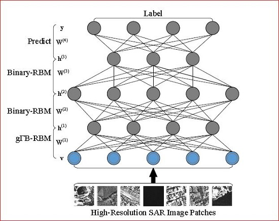
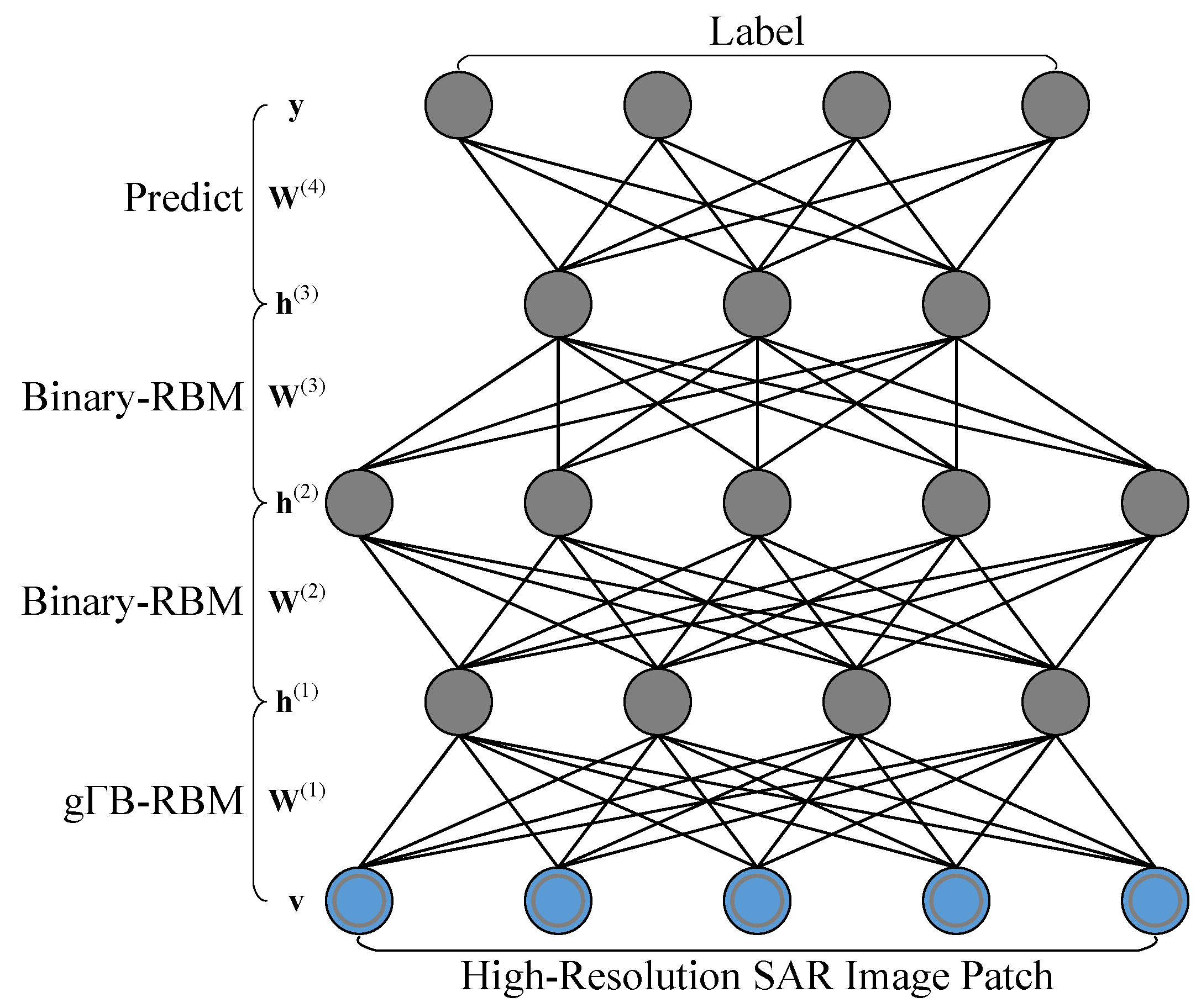
For the learned features, they can be used as the input of several supervised classifiers to produce category labels of SAR image samples, such as support vector machine, K-nearest neighbor and so on. As a hierarchical structure, it can be easily extended to a neural network by adding a prediction layer, in which a softmax classifier is employed to produce the discriminative information. Specifically, a discriminative neural network which consists of a four-layer g$\mathsf{\Gamma }$-DBN and one prediction layer is shown in Figure 2. It consists of three hidden layers ${\mathbf{h}}^{\left(1\right)}$, ${\mathbf{h}}^{\left(2\right)}$ and ${\mathbf{h}}^{\left(3\right)}$, which are formulated by three RBMs, including a g$\mathsf{\Gamma }$B-RBM and two standard binary RBMs, an input layer $\mathbf{v}$ for high-resolution SAR image samples and an output layer $\mathbf{y}$ for the category label. By feeding it with SAR image samples, the category label can be simply obtained by a feedforward inference on it. Similar to the work of Hinton et al. [45], training such a discriminative network is straightforward, which is implemented in Algorithm 2.

Algorithm 2 Formulating a Discriminative Network (DisNet)
Input:
1. Training SAR image samples: $\mathcal{V}={\left\{{\mathbf{v}}_p,y_p\right\}}_{p=1}^P$, where ${\mathbf{v}}_p\in {\left[0,1\right]}^m$ and $y_p\in \left\{1,2,\dots ,C\right\}$;
2. Number of units in each hidden layer: $n_1$, $n_2$, …, $n_h$;
Output: A discriminative neural network $\mathcal{N}$.
1:	Initialization: $n_0=P$;
2:	for$i=1$tohdo
3:	if $i=1$ then
4:	Training a g$\mathsf{\Gamma }$B-RBM ${\mathcal{R}}_1:\left\{{\mathbf{W}}^{\left(1\right)},{\mathbf{b}}^{\left(1\right)},{\mathbf{c}}^{\left(1\right)}\right\}$ with input $\left\{{\mathbf{v}}_1,{\mathbf{v}}_2,\dots ,{\mathbf{p}}_P\right\}$ and $n_1$ hidden nodes.
5:	Compute output ${\mathbf{h}}^{\left(1\right)}$ of the 1st RBM ${\mathcal{R}}_1$;
6:	else
7:	Training a stand binary RBM ${\mathcal{R}}_i:\left\{{\mathbf{W}}^{\left(i\right)},{\mathbf{b}}^{\left(i\right)},{\mathbf{c}}^{\left(i\right)}\right\}$ with input ${\mathbf{h}}^{\left(i-1\right)}$ and $n_i$ hidden units.
8:	Compute output ${\mathbf{h}}^{\left(i\right)}$ of the ith RBM ${\mathcal{R}}_i$;
9:	end if
10:	end for
11:	Unfold the RBM series to a neural network $\mathcal{N}:\left\{{\mathbf{W}}^{\left(1\right)},{\mathbf{W}}^{\left(2\right)},\dots ,{\mathbf{W}}^{\left(h\right)}\right\}$;
12:	Add a prediction layer $\mathbf{y}$ to $\mathcal{N}$ with C output nodes: $\mathcal{N}\leftarrow \left\{\mathcal{N},{\mathbf{W}}^{\left(h+1\right)}\right\}$, where ${\mathbf{W}}^{\left(h+1\right)}$ is initialized randomly;
13:	Tune weights of the neural network $\mathcal{N}$ with labels $y_1,y_2,\dots ,y_P$ via a backpropagation procedure.
14:	return$\mathcal{N}:\left\{{\mathbf{W}}^{\left(1\right)},{\mathbf{W}}^{\left(2\right)},\dots ,{\mathbf{W}}^{\left(h+1\right)}\right\}$.

Specifically, there are two major parts of Algorithm 2, which are RBMs learning (in step 2–step 10) and discriminative neural network construction and fine tuning (in step 11–step 13). Two kinds of RBMs are trained in this work for high-resolution SAR image statistical modeling, which are the g$\mathsf{\Gamma }$B-RBM (in step 4) and standard binary RBMs (in step 7). After stacking these RMBs in a hierarchal manner, the learned g$\mathsf{\Gamma }$-DBN is unfolded to a neural network $\mathcal{N}$ (in step 11) and followed by adding a prediction layer (in step 12). The weight matrix ${\mathbf{W}}^{\left(h+1\right)}$ of the prediction is initialized randomly. In the last step (step 13), all of these weight matrix are tuned according to the labeling information of the training high-resolution SAR image samples. With the learned discriminative neural network, the category label $y_p$ of each SAR image sample ${\mathbf{v}}_p$ can be obtained via a simple feedforward pass.

Besides, two aspects of the computational complexity, i.e., memory and computations, are also employed to investigate the learning algorithm of discriminative network (denoted as DisNet). In this work, the formulated DisNet consists of h RBMs, i.e., a g$\mathsf{\Gamma }$B-RBM and $h-1$ binary RBMs. During training, the DisNet starts out fully connected leading to a total number of weights to $N_w={\sum }_{i=1}^{h-1}{n}_i{n}_{i+1}$. The computation and memory costs are highly relatively to number of non-zero weights. However, the computational cost of neuron is heavily depend on the selective activation function and summation operations. After training the DisNet with a fully connected structure, the network goes through a supervised phase where connections are fine-tuned via a backpropagation procedure. In summary, the overall computational cost depends on architecture of the learned DisNet: the number of layers and the number of neurons per hidden layer which affect the number of weight connections.

2.3. Discussions of the Proposed Approach

Apart from traditional probability mixture models [5,46,47,48], the other mixture models, which are named topic models [49,50,51], are also utilized to characterize the content of SAR images. They are based on the assumption that each SAR image can be represented as a mixture of topics, in which each topic is determined by a probability distribution over some words. As the inference is intractable, posterior distribution over topics have been approximated inaccurately and slowly in the topic models. Compared with these mixture approaches, the major advantage of the proposed approach is due to the fact that it can learn a nonlinear distributed representation of SAR images in a hierarchical manner. While handling high-resolution SAR images, the major characteristics of the proposed approach are listed as follows.

• After casting the proposed g$\mathsf{\Gamma }$B-RBM as a mixture model, the likelihood and model parameters can be effectively approximated via a simple gradient-based optimization (as shown in Algorithm 1). It needs less computation and easier to implement than traditional EM procedure in the probability mixture models.
• With a layer-by-layer representation, high-level representation can be generated by exploiting higher-order and nonlinear distributions of SAR images.
• As shown in Algorithm 2, the discriminative network is formulated by an unsupervised training of RBMs and supervised parameter tuning. It is easy to implement in a greedy and hierarchical manner.

Besides, the proposed g$\mathsf{\Gamma }$-DBN first takes advantages of an effective layer-by-layer greedy learning strategy into initialize the deep network, and then fine-tunes all of the weights jointly with the desired category labels. It can be utilized to learn the statistical characterizes of SAR images and used to distinct different land-covers by building a deep hierarchical structure. As its basic blocks, the RBMs are famous for their powerful expression and tractable inference. However, training an RBM can be difficult in practice due to the intractability of the log-likelihood computation. Exact computation requires an unbiased sampling from the model distribution for a long time to ensure convergence to stationarity, which is of exponential complexity. A Gibbs sampling procedure is employed to approximate the log-likelihood of RBM (in Algorithm 1) from training data. Different from CNNs which are inspired by biological process in that the connectivity pattern between neurons resemble the organization of visual cortex, the proposed g$\mathsf{\Gamma }$-DBN is a deep generative model to learning distribution of SAR images in a unsupervised manner. Specifically, a simple comparison between g$\mathsf{\Gamma }$-DBN and some CNN-based approaches for remote sensing image processing is listed in

Table 1. Comparison of the g$\mathsf{\Gamma }$-DBN and CNN-based approaches.

	g$\mathsf{\Gamma }$-DBN	CNN-Based Approaches [19,20,21,24,52]
Model	generative model	biological-inspired
Configuration	g$\mathsf{\Gamma }$B-RBM Binary-RBMs	convolutional layers pooling layers full-connection layers
Training	unsupervised training fine-tuning	dropout & dropconnect data augmentation pre-training & fine-tining low-rank & tensor decomposition

.

Finally, the speckle phenomenon in SAR images makes their visual and automatic interpretation a difficult task, especially in a high-resolution case. Some multilook preprocessing could be considered to reduce strong fluctuations of SAR images for land-cover classification, such as spatial multilooking and temporal mutilooking. For spatial multilooking [53], the speckle variance reduction is obtained at the cost of a resolution loss after averaging pixel values within a sliding window. However, the use of multiple SAR images taken over the same scene during a relatively short period of time, i.e., temporal multilooking [54,55], allows for a continuous monitoring of the earth surface. For multitemporal SAR images, some areas, like buildings and homogeneous fields, the spatial response remains unchanged over short period. It offers great importance for both land-cover classification and for the analysis of environmental changes. In this paper, we just focusing on the statistical modeling of single high-resolution SAR image via the proposed g$\mathsf{\Gamma }$-DBN and utilized to distinguish different land-covers.

3. Experimental Results and Discussions

To investigate classification performance of the proposed approach, several approaches are adopted in this experiment for comparison. Specifically, they are listed as follows.

• Patch Vector—Similar to the work of Varma et al. [56], a simple patch vector based descriptor is utilized as the basic feature to characterize SAR image samples. It just simply keeping the raw pixel intensities of a square neighborhood to form a feature vector.
• GLCM + Gabor [57]—In this experiment, some statistics of GLCM and responses of Gabor filters are employed to characterize SAR image samples. The statistics computed by the GLCM are energy, entropy, roughness, contrast and correlations. Meanwhile, the means and standard deviations of the magnitude of the Gabor filtering responses with 3-scales and 4-orientations are utilized in this experiment.
• DBN [45,58]—The classical DBN with Gaussian distribution is also used in this experiment to evaluate performance of the proposed approach.

For the patch vector and GLCM + Gabor, a linear kernel based SVM (Available from: http://www.csie.ntu.edu.tw/~cjlin/libsvm) [59] is utilized in classify these features. For DBN and the proposed g$\mathsf{\Gamma }$-DBN, a softmax layer is add on the last layer to generate labels for different land-covers.All of these experiments are conducted on a PC with Intel Core I3 CPU and 4G memory, and implemented over Matlab 2014a.

3.1. Performance Evaluation over Patch Sets

3.1.1. Datasets and Settings

In order to evaluate the quality of the proposed approach, six high-resolution SAR image patche sets are formulated in this experiment in different patch sizes. Specifically, they are captured from four typical scenes (shown in Figure 3), which are water (WA), farmland (FL), vegetation (VG) and buildings (BD). All of these four scenes are captured bu ALOS PALSAR-2 satellite with a HH-polarization spotlight mode.

From each scene, 15,000 patches are selected randomly to formulate each patch set in an overlapping manner. Therefore, there are totally 60,000 SAR image patches in each set. Details of the constructed patch sets are listed in

Table 2. Details of 6 high-resolution SAR image patch sets.

Dataset	ptSet1	ptSet2	ptSet3	ptSet4	ptSet5	ptSet6
Size of image patch	21 × 21	25 × 25	29 × 29	33 × 33	37 × 37	41 × 41
Num. of patches	15,000 × 4

. Meanwhile, the power parameter of g$\mathsf{\Gamma }$-DBN is setting as 2 in all of the following experiments.

3.1.2. Results and Analysis

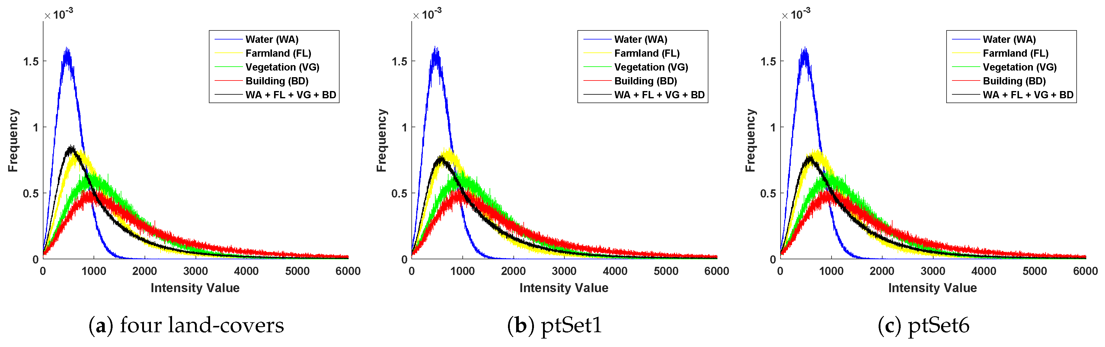
First of all, intensity histograms of these four scenes (Figure 3) are shown in Figure 4a. Heavy-tail could be observed from histograms of these four scenes, which is difficult to characterized via a simple probability distribution model. It can also be observed from Figure 4a that the vegetation and building areas have similar statistical properties as a result of complex backscatters. Because of its simple spatial structure, water areas could be distinguished effectively from the other land-covers. Meanwhile, intensity histograms of four land-covers of two selected SAR patch sets, i.e., ptSet1 and ptSet2, are also drawn in Figure 4b,c respectively. Similar to Figure 4a, heavy-tails can also be observed from these two patch sets for different land-covers. In the following section, we mainly check the classification capacity of the proposed approach over these six patch sets.

Then, the average classification accuracies of g$\mathsf{\Gamma }$-DBN is checked. In this experiment, 10,000 patches which are selected randomly from each patch set are utilized to learn a 4-layer g$\mathsf{\Gamma }$-DBN with 2 hidden layer, which has 100 units in the first hidden layer and 20 units in the second hidden layer. The remaining 5000 patches of each patch set are employed for testing. After conducting this experiment 20 times independently, the average classification accuracies (mean and standard variation) of the learned g$\mathsf{\Gamma }$-DBN on each patch set is shown in

Table 3. Mean and standard variation of classification accuracies (100%) of different approaches over each patch set.

Dataset	ptSet1	ptSet2	ptSet3	ptSet4	ptSet5	ptSet6
Patch Vector	48.30 ± 1.17	46.10 ± 1.50	44.78 ± 0.97	43.15 ± 1.15	42.97 ± 0.86	42.09 ± 1.31
GLCM + Gabor	64.62 ± 0.51	66.50 ± 0.47	68.44 ± 0.63	70.95 ± 0.37	72.45 ± 0.61	73.40 ± 0.41
DBN	60.72 ± 1.21	62.18 ± 0.44	66.43 ± 0.48	67.18 ± 0.58	67.41 ± 0.69	67.88 ± 1.60
gΓ-DBN	68.21 ± 3.18	69.75 ± 2.08	72.05 ± 0.86	73.14 ± 1.35	74.32 ± 0.94	75.56± 0.83

. It can be observed that the highest classification accuracy is reached on ptSet6 comparing with the other approaches. For GLCM + Gabor, DBN and gΓ-DBN, classification accuracies are increased with the size of local patches because richer information could be captured from different land-covers with a larger patch size. Conversely, the classification accuracy of Patch Vector is decreasing from ptSet1 to ptSet6, which mainly be caused by the following two facts. On one hand, as the dimension of features is increased quadratically with the size of local patch (i.e., $21\times 21$ for ptSet1 and $41\times 41$ for ptSet6), it need a large number of training samples to training an effective SVM model. On the other hand, a liner-kernel is one of the simplest choice of SVM model, which could not capture enough discriminant information to classify each SAR patch. Because the major focuses of this work is to evaluate the effectiveness of features generated by different approaches, the choice of linear-SVM with general settings is enough in this experiment.

In order the view the discrimination capacity of these four approaches, some confusing matrices over ptSet2 are drawn in Figure 5. It can be observed that the classification accuracy of water area is higher than the other categories as a result of its simple spatial structure. For vegetation area, the best classification accuracy is achieved by the proposed g$\mathsf{\Gamma }$-DBN. Because of its complex and clutter spatial structures, much misclassification of the vegetation and building areas can be observed from the confusing matrix of patch vector (shown in Figure 5a). At the same time, classification accuracies of building areas appear fairly well in GLCM + Gabor (Figure 5b), DBN (Figure 5c) and the proposed g$\mathsf{\Gamma }$-DBN approaches (Figure 5d). As a result of their complex spatial structures and variety of the backscatters, it is difficult to capture enough information to characterize them except for water areas.

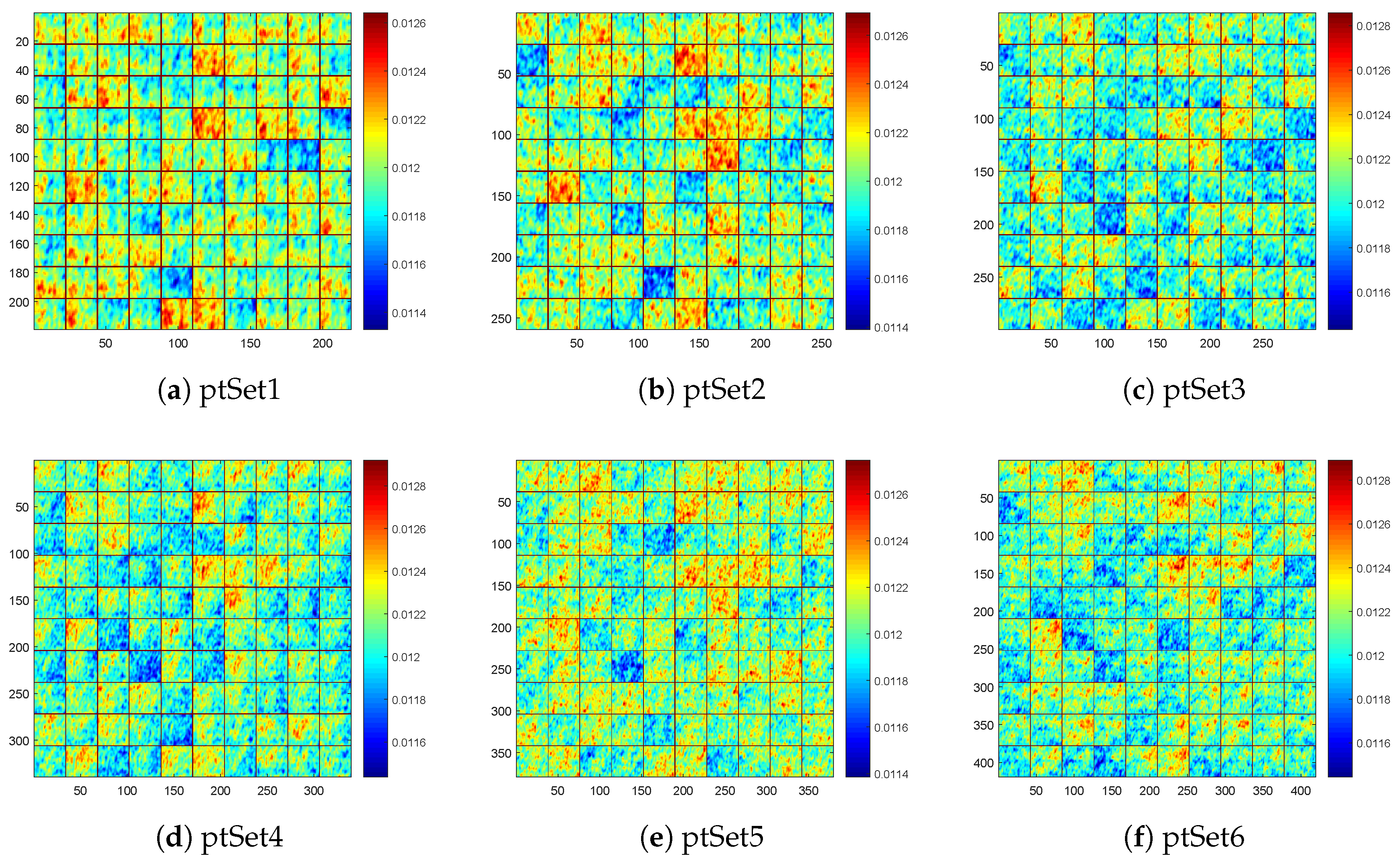
To going deeper of the proposed g$\mathsf{\Gamma }$-DBN, each hidden unit can be observed as one feature detector of the input local high-resolution SAR image patches in the former section. It can be visualized as a collection of the bases that resemble Gabor filters [60], in which each component of parameter $\mathbf{W}$ is also referred as a receptive field. As the basic element of g$\mathsf{\Gamma }$-DBN, the g$\mathsf{\Gamma }$B-RBM is directly related to high-resolution SAR image patches. It is investigated in this experiment to view the capacity of feature learning. Specifically, the parameter $\mathbf{W}$ of g$\mathsf{\Gamma }$B-RBM which is learned by a 1-step contrastive divergence algorithm from all of these patch sets are shown in Figure 6 respectively. It can be observed from Figure 6 that some interesting structures are appeared, such as part of edge, orientation, and speckle-like structures, which are distributed widely in high-resolution SAR scenes. With an increased number of the hidden units of g$\mathsf{\Gamma }$B-RBM, plentiful spatial structures would be appeared to characterize these high-resolution SAR images.

Besides, the discriminative capacity of g$\mathsf{\Gamma }$-DBN is also checked in this experiment. Specifically, six confusion matrices over different patch sets are shown in Figure 7. As a result of the water clutter response, the classification accuracy of water in dataset ptSet1 is the smallest one. Meanwhile, classification accuracy of building areas reach the highest value on ptSet5 and ptSet6 (shown in Figure 7e,f). As shown in Figure 7d–f, it is difficult to distinguish vegetation and building materials as a result of its complex backscatter. In general, it can be noticed form all of these confusion matrices that the proposed g$\mathsf{\Gamma }$-DBN have preferable capacity to characterize different land-covers.

Finally, the computation burden of land-cover classification system mainly located in the procedure of feature extraction and classifier training. Specifically, the average CPU times of these approaches are also recorded and listed in

Table 4. CPU times (s) for the g$\mathsf{\Gamma }$-DBN on each SAR image patch set (ft. ext. for feature extraction, SVM tr. for SVM training, DBN tr. DBN Training) and DisNet for discriminant network formulation.

Approaches	CPU Times	ptSet1	ptSet2	ptSet3	ptSet4	ptSet5	ptSet6
Patch Vector	ft. ext.	–
	SVM tr.	1.12 × ${10}^3$	1.13 × ${10}^3$	1.15 × ${10}^3$	1.14 × ${10}^3$	1.14 × ${10}^3$	1.15 × ${10}^3$
GLCM + Gabor	ft. ext.	661.41	653.92	671.01	661.35	679.68	671.69
	SVM tr.	198.23	211.55	197.10	193.69	185.32	191.12
DBN	DBN tr.	2.94	3.84	6.04	7.23	7.48	9.21
	DisNet	1.81	2.36	3.82	3.89	5.26	6.35
gΓ-DBN	gΓ-DBN tr.	7.63	9.90	12.79	15.56	19.68	34.73
	DisNet	6.79	8.29	10.77	12.37	19.08	28.67

after 20 times independently running. It can be noticed that feature extraction procedure in GLCM + Gabor approach consumes the most of CPU times, because the texture descriptors are computed in a patch-wise manner. Nevertheless, the CPU times for SVM model training is not changed seriously for GLCM + Gabor approach on different patch sets. The main reason for this is that the texture descriptor of each local SAR image patch have the same number of elements. Furthermore, it can also be noticed in Table 4 that CPU times for SVM model training is increased rapidly for Patch Vector approach because of the fact that dimension of features is increased quadratically with the size of local patches. Due to the advantage of simple gradient approximation in K-CD optimization and a batch-wised trick, CPU times of DBN and g$\mathsf{\Gamma }$-DBN is significantly less than that of the other approaches. Although the classifier could be trained in advance in an off-line manner, the feature extraction still be conducted on-line while performing land-cover classification. Therefore, a large amount of CPU times is still needed to capture local features, such as the texture descriptors computed by GLCM + Gabor approach in this experiment.

3.2. Performance Evaluation over Large-Scale SAR Images

In this experiment, two large-scale SAR images are utilized to evaluate performance of the proposed approach.

3.2.1. Barcelona Image

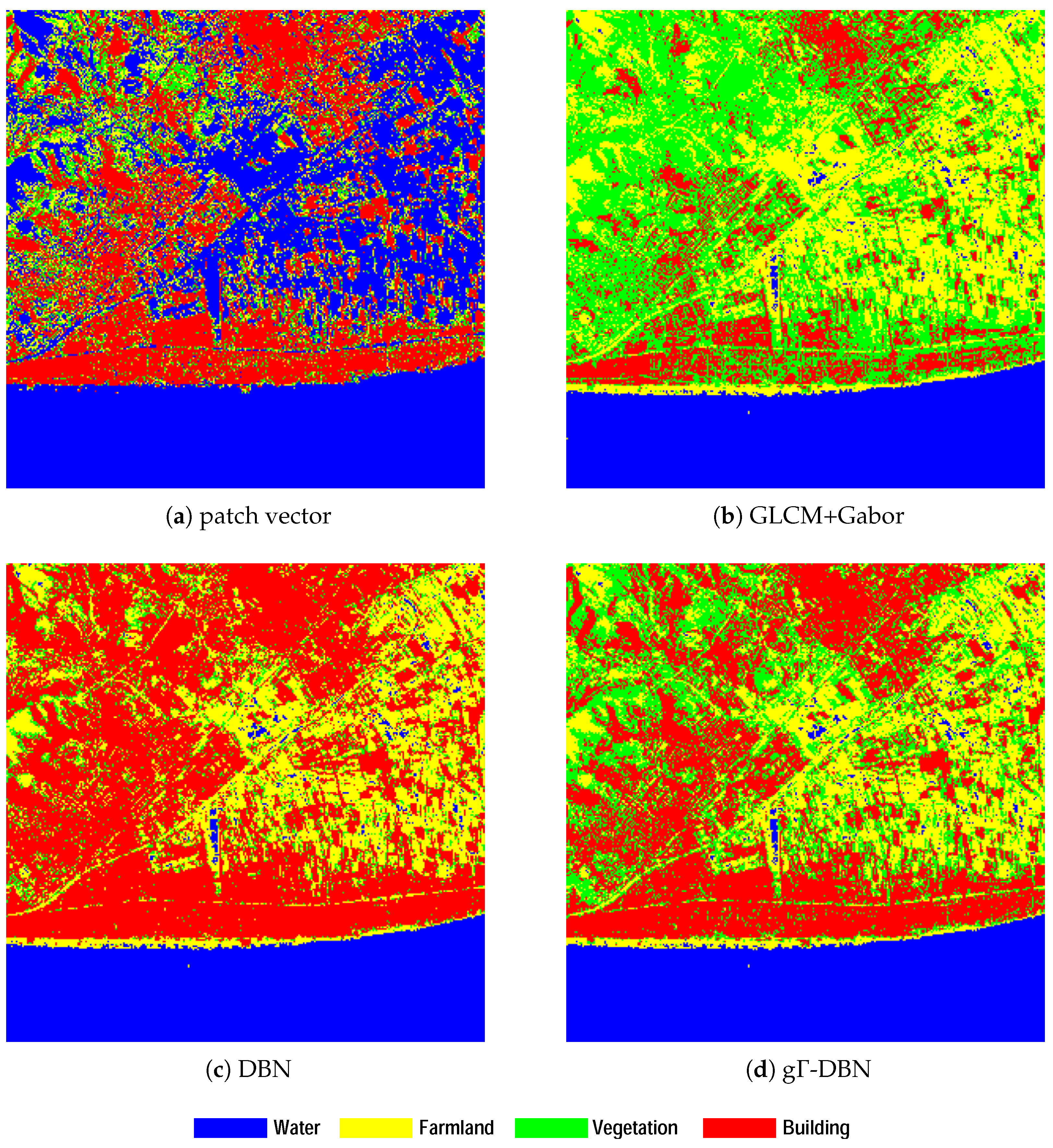
In the first experiment, the Barcelona image (left part in Figure 8) is utilized in this experiment to evaluate th performance of the proposed approach. It is captured by L-band ALOS PALSAR-2 satellite on 22 September 2014 with HH-polarization spotlight mode over Barcelona city in Spain. It has 10,000 × 1000 pixels in size with a ground resolution of 1.0 m. The reference land-cover of the Barcelona image with the same area is also captured from GoogleEarth in the same period and shown in the right part of Figure 8. Specifically, a four-category land-cover classification problem is conducted on Barcelona image in this experiment, i.e., water, farmland, vegetation and buildings, which is the same as the former experiment. To generate a patch-wise land-cover labeling, parameters of this experiment are setting as follows.

• Firstly, the Barcelona image is partitioned into 91,809 local patches in a non-overlapping manner, in which each one has 33 × 33 pixel in size. The patch set ptSet4 formulated in Table 2 are utilized for model training for all of these four approaches.
• The power parameter $\beta$ of the generalized Gamma distribution is setting as 2.
• In this experiment, a four layer DBN and g$\mathsf{\Gamma }$-DBN is trained for land-cover classification. It consists of one input layer, two hidden layer and one output layer. Specifically, the number of units of input layer is 1089, corresponding to each local patch. Meanwhile, the number of units in each hidden layer is setting as 200 and 20 respectively. The output layer has 4 nodes for different land-covers.

Classification results of different approaches are shown in Figure 9a–d respectively.

It can be observed from these results that the large water area lies at the bottom of Barcelona image is clearly labeled by all of these approaches. However, much misclassification was occurred at the rod-like pond area as a result of heavy noise by strong scatter beside it. For the classification result of Patch Vector (Figure 9a), a large part of farmland areas which lies in the center right part is misclassified as water. It may be caused by the fact that a linear kernel is insufficient to distinguish the farmland and water when they have similar intensity values. As a result of its difference to water, building materials are clearly labeled by patch vector with a linear-kernel SVM. Meanwhile, it can also be observed from Figure 9b that classification result of GLCM + Gabor with linear-kernel SVM appear well in a large part of the vegetation areas, especially at the ridge area in the top-left part on the Barcelona image. However, a large amount of building areas are failed to detect in Figure 9b. Because of its non-Gaussian characterizes, classification results of DBN (shown in Figure 9c) is even worse than the classification result of Figure 9b. Comparing with the other three approaches, it can be noticed that the g$\mathsf{\Gamma }$-DBN (shown in Figure 9d) performs well on the building and farmland areas.

Besides, the computational cost is also one of the most important factors for SAR image land-cover classification. Specifically, CPU times is also recorded in this experiment while labeling Barcelona image, which are listed in

Table 5. CPU times (s) for Barcelona image classification with different approaches.

	Patch Vector	GLCM + Gabor	DBN	g$\mathsf{\Gamma }$-DBN
Patch partition	3.85
Feature Extraction	0	1.31 × 10${}^3$	0	0
Classification	1.14 × 10${}^3$	307.31	6.79	7.94

. It can be observed that DBN and g$\mathsf{\Gamma }$-DBN need only a light CPU times to label all of the local SAR image patches via a simple feed-forward pass on the learned discriminant network. However, for the linear-kernel based SVM, much CPU times are required fro decision cost function computation, which is increased quickly with the feature dimension. Therefore, the CPU times of GLCM + Gabor approach is much time-consuming one compared with the other three approaches in this experiment.

3.2.2. Napoli Image

In the second experiment, the Napoli image (shown in left part of Figure 10a) is utilized to evaluate the performance of the proposed approach. It was captured by X-band COSMO-SkyMed satellite on 1 March 2013 with a HH-polarization HIMAGE model over the Napoli area in Italiana. It has 4000 × 6000 pixels in size with a ground resolution of 3.0 m. There are three major land-covers in this image, which are water, openlands and buildings. Intensity histograms of three selected sub-regions, which are water openland and building, are shown in Figure 10b respectively. Meanwhile, the intensity histogram of the whole Napoli image is also computed and plotted in Figure 10b. Heavy-tails can be observed from all of these histograms, which appears sensible non-Gaussian characteristics. To obtain a patch-wise classification result of Napoli image, parameters of the g$\mathsf{\Gamma }$-DBN are setting as follows.

• Firstly, the Napoli image is partitioned into 295,704 patches in a non-overlapping manner, in which each one has 9 × 9 pixels in size. At the same time, 30,000 local patches which are randomly captured from three marked areas (shown in Figure 10a) are employed to learn the g$\mathsf{\Gamma }$-DBN, in which 10,000 patches per each category.
• In this experiment, the power, i.e., $\beta$, of g$\mathsf{\Gamma }$D (in Equation (1)) is also setting as 2.
• In this experiment, a three layer g$\mathsf{\Gamma }$-DBN is learned form the selected training samples. It has one hidden layer with 20 units. Numbers of units of the input and output layers are setting as 81 and 3 respectively, which are corresponding the input SAR image patch (9 × 9) and land-covers should be labeled.

With the learned g$\mathsf{\Gamma }$-DBN, classification result of Napoli image is shown in Figure 10c.

It can be noticed that different categories of SAR land-covers could be distinguished effectively via the proposed g$\mathsf{\Gamma }$-DBN. Form Figure 10, it can be observed that some hangar-like structures are misclassified as waters. Some roads between these hangar-like structures are labeled as building materials as a result of strong backscatter. Meanwhile, it can also be observed from Figure 10c that buildings and openland areas could be marked effectively via the proposed approach. Besides, the CPU times is much less because a small local SAR image patch size which is utilized for Napoli image classification. Specifically, it just needs 2.05 s for local image patch partition and 3.1 s for image classification in this experiment.

3.3. Discussions

In this section, some aspects of g$\mathsf{\Gamma }$-DBN are discussed via several experiments. Specifically, the local SAR image patch set ptSet4 in Table 2 is utilized to evaluate classification performance of the proposed approach, in which 10,000 patches of each category is employed to learn a discriminative network and other 5000 samples for testing.

Firstly, we check the classification accuracy of the g$\mathsf{\Gamma }$-DBN with respect to power parameter $\beta$ in g$\mathsf{\Gamma }$D (Equation (1)). In particular, a g$\mathsf{\Gamma }$-DBN with 2 hidden layers is learned in this experiment, which have 400 and 40 nodes respectively. With different settings of $\beta$, the average accuracies of g$\mathsf{\Gamma }$-DBN over dateset over patch set ptSet4 are shown in Figure 11 after conducting each experiment 10 times independently. It can be noticed that the accuracy over ptSet4 appears much stable with power parameter $\beta$. Meanwhile, the highest classification accuracy is reached with setting $\beta =2$.

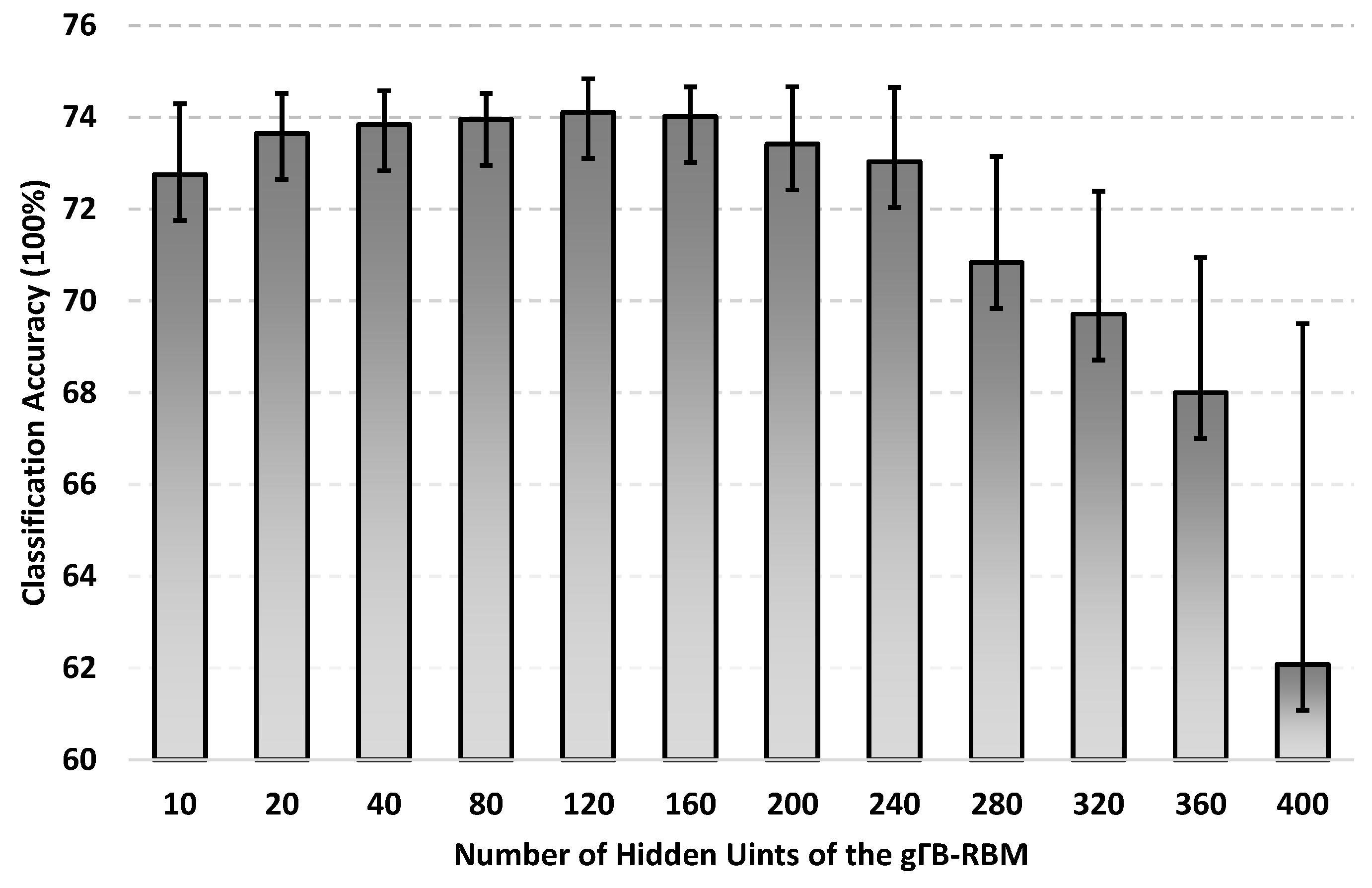
Secondly, the number of hidden units of g$\mathsf{\Gamma }$B-RBM is checked in this experiment after casting it as a special probability mixture model for high-resolution SAR images. In g$\mathsf{\Gamma }$B-RBM, each hidden unit can be viewed as one choice of different mixture strategies. Therefore, the average accuracies of g$\mathsf{\Gamma }$B-RBM on ptSet4 is checked with different number of hidden units in this experiment. Specifically, the number of hidden units is setting as 10, 20, 40, 80, 120, 160, 200, 240, 280, 320, 360 and 400 respectively. With a 3-layer discriminative neural network which is constructed by stacking a g$\mathsf{\Gamma }$B-RBM and a predict layer, the average classification accuracies are shown in Figure 12 after conducting this experiment 10 times independently. It can be observed that the classification accuracy is increased with the number of hidden units, as it can capture enough statistical relations from high-resolution SAR images with a large number of hidden units. However, classification accuracies are dripped quickly with a larger number of hidden units. It is caused by the fact that number of units in the predict layer is only 4, which is may be much smaller to capture enough statistical relations between these hidden units. It can be noticed from Figure 12 that the highest classification accuracy is reached with 120 hidden units while just employing a g$\mathsf{\Gamma }$B-RBM for dataset ptSet4 classification.

Lastly, choices on number of hidden layers and units in each hidden layer are checked in this experiment. Specifically, the discriminative network formulated by g$\mathsf{\Gamma }$-DBN has 1089 and 4 units in the input and output layer respectively. They are corresponding to the size of local SAR image patches with 33 × 33 pixels and 4 different land covers should be distinguished. After conducting the experiment 10 times independently, the average accuracies and CPU times for model training and classification are listed in

Table 6. Average classification accuracies and CPU times for model training and testing with different number of hidden layers and units in each layer.

Hidden Layers	Num. of Units	Accuracy (100%)	CPU Times (s)
			Model Training	Testing
1	[1089, 100, 4]	72.54 ± 1.15	20.01 ± 0.68	0.31 ± 0.01
2	[1089, 400, 20, 4]	73.22 ± 1.01	69.75 ± 3.78	0.92 ± 0.04
3	[1089, 400, 100, 20, 4]	72.71 ± 1.35	79.13 ± 3.35	1.17 ± 0.13
4	[1089, 400, 200, 100, 20, 4]	71.61 ± 1.43	87.83 ± 5.23	1.23 ± 0.29

for different settings of hidden layers and units. It can be observed that the highest classification accuracy is reached when it has 2 hidden layers with 400 and 20 units respectively. Meanwhile, it can also be noticed that the CPU times for model training and testing is also increased with the number of hidden layers, as it will need much layer inference to generate the final category label. Nevertheless, the CPU time-consuming is not increased serious with the number of hidden layers.

4. Conclusions and Further Works

In this paper, a g$\mathsf{\Gamma }$-DBN is formulated by stacking a g$\mathsf{\Gamma }$B-RBM and several standard binary RBMs to model the statistical characteristics for high-resolution SAR image land-cover classification. The high-order statistical relations of SAR images can be exploited effectively via the proposed framework. At the same time, it can be used for distinguishing different land-covers by adding an additional predict layer. Experimental results on some local SAR image patch sets and large-scale scenes illustrate the effectiveness and robustness of the proposed approach. However, there are still some limits of the proposed approach, such as how to choose an appropriate number of hidden layer to capture enough discriminant information for different land-covers and more effective training approach for model parameters. All of these will be considered in our future works.

References

- Liao, C.; Wang, J.; Shang, J.; Huang, X.; Liu, J.; Huffman, T. Sensitivity Study of Radarsat-2 Polarimetric SAR to Crop Height and Fractional Vegetation Cover of Corn and Wheat. Int. J. Remote Sens. 2018, 39, 1475–1490. [Google Scholar] [CrossRef]
- Tsyganskaya, V.; Martinis, S.; Marzahn, P.; Ludwig, R. SAR-based Detection of Flooded Vegetation—A Review of Characteristics and Approaches. Int. J. Remote Sens. 2018, 39, 2255–2293. [Google Scholar] [CrossRef]
- Montazeri, S.; Gisinger, C.; Eineder, M.; Zhu, X. Automatic Detection and Positioning of Ground Control Points Using TerraSAR-X Multiaspect Acquisitions. IEEE Trans. Geosci. Remote Sens. 2018, 56, 2613–2632. [Google Scholar] [CrossRef]
- Gohil, B.S.; Sikhakolli, R.; Gangwar, R.K.; Kumar, A.S.K. Oceanic Rain Flagging Using Radar Backscatter and Noise Measurements from Oceansat-2 Scatterometer. IEEE Trans. Geosci. Remote Sens. 2016, 54, 2050–2055. [Google Scholar] [CrossRef]
- Li, H.C.; Krylov, V.A.; Fan, P.Z.; Zerubia, J.; Emery, W.J. Unsupervised Learning of Generalized Gamma Mixture Model With Application in Statistical Modeling of High-Resolution SAR Images. IEEE Trans. Geosci. Remote Sens. 2016, 54, 2153–2170. [Google Scholar] [CrossRef]
- Sportouche, H.; Nicolas, J.M.; Tupin, F. Mimic Capacity of Fisher and Generalized Gamma Distributions for High-Resolution SAR Image Statistical Modeling. IEEE J. Sel. Top. Appl. Earth Obs. Remote Sens. 2017, 10, 5695–5711. [Google Scholar] [CrossRef]
- Barreto, T.L.M.; Rosa, R.A.S.; Wimmer, C.; Moreira, J.R.; Bins, L.S.; augo Menocci Cappabianco, F.; Almeida, J. Classification of Detected Changes from Multitemporal High-Resolution X-band SAR Images: Intensity and Texture Descriptors from SuperPixels. IEEE J. Sel. Top. Appl. Earth Obs. Remote Sens. 2016, 9, 5436–5448. [Google Scholar] [CrossRef]
- Bahmanyar, R.; Cui, S.; Datcu, M. A Comparative Study of Bag-of-Words and Bag-of-Topics Models of EO Image Patches. IEEE Geosci. Remote Sens. Lett. 2015, 12, 1357–1361. [Google Scholar] [CrossRef] [Green Version]
- Pan, Z.; Qiu, X.; Huang, Z.; Lei, B. Airplane Recognition in TerraSAR-X Images via Scatter Cluster Extraction and Reweighted Sparse Representation. IEEE Geosci. Remote Sens. Lett. 2017, 14, 112–116. [Google Scholar] [CrossRef]
- Moser, G.; Zerubia, J.; Serpico, S.B. Dictionary-Based Stochastic Expectation-Maximization for SAR Amplitude Probability Density Function Estimation. IEEE Trans. Geosci. Remote Sens. 2006, 44, 188–200. [Google Scholar] [CrossRef]
- Kayabol, K.; Voisin, A.; Zerubia, J. SAR Image Classification with Non-stationary Multinomial Logistic Mixture of Amplitude and Texture Densities. In Proceedings of the 18th IEEE International Conference on Image Processing, Brussels, Belgium, 11–14 September 2011; pp. 169–172. [Google Scholar]
- Peng, Q.; Zhao, L. SAR Image Filtering Based on the Cauchy–Rayleigh Mixture Model. IEEE Geosci. Remote Sens. Lett. 2014, 11, 960–964. [Google Scholar] [CrossRef]
- Song, W.; Li, M.; Zhang, P.; Wu, Y.; Tan, X.; An, L. Mixture WG Γ-MRF Model for PolSAR Image Classification. IEEE Trans. Geosci. Remote Sens. 2018, 56, 905–920. [Google Scholar] [CrossRef]
- LeCun, Y.; Bengio, Y.; Hinton, G. Deep learning. Nature 2015, 521, 436–444. [Google Scholar] [CrossRef] [PubMed]
- Gonzalez-Garcia, A.; Modolo, D.; Ferrari, V. Do Semantic Parts Emerge in Convolutional Neural Networks? Int. J. Comput. Vis. 2018, 126, 476–494. [Google Scholar] [CrossRef]
- Zhang, L.; Zhang, L.; Du, B. Deep Learning for Remote Sensing Data: A Technical Tutorial on the State of the Art. IEEE Geosci. Remote Sens. Mag. 2016, 4, 22–40. [Google Scholar] [CrossRef]
- Zhu, X.X.; Tuia, D.; Mou, L.; Xia, G.S.; Zhang, L.; Xu, F.; Fraund, F. Deep Learning in Remote Sensing: A Comprehensive Review and List of Resources. IEEE Geosci. Remote Sens. Mag. 2017, 5, 8–36. [Google Scholar] [CrossRef] [Green Version]
- Geng, J.; Fan, J.; Wang, H.; Ma, X.; Li, B.; Chen, F. High-Resolution SAR Image Classification via Deep Convolutional Autoencoders. IEEE Geosci. Remote Sens. Lett. 2015, 12, 2351–2355. [Google Scholar] [CrossRef]
- Chen, S.; Wang, H.; Xu, F.; Jin, Y.Q. Target Classification Using the Deep Convolutional Networks for SAR Images. IEEE Trans. Geosci. Remote Sens. 2016, 54, 4806–4817. [Google Scholar] [CrossRef]
- Huang, Z.; Pan, Z.; Lei, B. Transfer Learning with Deep Convolutional Neural Network for SAR Target Classification with Limited Labeled Data. Remote Sens. 2017, 9, 907. [Google Scholar] [CrossRef]
- Makantasis, K.; Karantzalos, K.; Doulamis, A.; Doulamis, N. Deep Supervised Learning for Hyperspectral Data Classification through Convolutional Neural Networks. In Proceedings of the IEEE International Geoscience and Remote Sensing Symposium (IGARSS), Milan, Italy, 26–31 July 2015; pp. 4959–4962. [Google Scholar]
- De, S.; Bruzzone, L.; Bhattacharya, A.; Bovolo, F.; Chaudhuri, S. A Novel Technique Based on Deep Learning and a Synthetic Target Database for Classification of Urban Areas in PolSAR Data. IEEE J. Sel. Top. Appl. Earth Obs. Remote Sens. 2018, 11, 154–170. [Google Scholar] [CrossRef]
- Zhang, Z.; Wang, H.; Xu, F.; Jin, Y.Q. Complex-Valued Convolutional Neural Network and Its Application in Polarimetric SAR Image Classification. IEEE Trans. Geosci. Remote Sens. 2017, 55, 7177–7188. [Google Scholar] [CrossRef]
- Makantasis, K.; Doulamis, A.; Doulamis, N.; Nikitakis, A.; Voulodimos, A. Tensor-based Nonlinear Classifier for High-Order Data Analysis. arXiv, 2018; arXiv:1802.05981. [Google Scholar]
- Qu, J.; Lei, J.; Li, Y.; Dong, W.; Zeng, Z.; Chen, D. Structure Tensor-Based Algorithm for Hyperspectral and Panchromatic Images Fusion. Remote Sens. 2018, 10, 373. [Google Scholar] [CrossRef]
- Huang, X.; Qiao, H.; Zhang, B.; Nie, X. Supervised Polarimetric SAR Image Classification Using Tensor Local Discriminant Embedding. IEEE Trans. Image Process. 2018, 27, 2966–2979. [Google Scholar] [CrossRef]
- Salakhutdinov, R. Learning Deep Generative Models. Ann. Rev. Stat. Appl. 2015, 2, 361–385. [Google Scholar] [CrossRef] [Green Version]
- Zhong, P.; Gong, Z.; Li, S.; Schönlieb, C.B. Learning to Diversify Deep Belief Networks for Hyperspectral Image Classification. IEEE Trans. Geosci. Remote Sens. 2017, 55, 3516–3530. [Google Scholar] [CrossRef]
- Zhang, N.; Ding, S.; Zhang, J.; Xue, Y. An Overview on Restricted Boltzmann Machines. Neurocomputing 2018, 275, 1186–1199. [Google Scholar] [CrossRef]
- Cui, Z.; Cao, Z.; Yang, J.; Ren, H. Hierarchical Recognition System for Target Recognition from Sparse Representations. Math. Probl. Eng. 2015, 2015. [Google Scholar] [CrossRef]
- Liu, F.; Jiao, L.; Hou, B.; Yang, S. POL-SAR Image Classification Based on Wishart DBN and Local Spatial Information. IEEE Trans. Geosci. Remote Sens. 2016, 54, 3292–3308. [Google Scholar] [CrossRef]
- Qin, F.; Guo, J.; Sun, W. Object-oriented Ensemble Classification for Polarimetric SAR Imagery Using Restricted Boltzmann Machines. Remote Sens. Lett. 2017, 8, 204–213. [Google Scholar] [CrossRef]
- Zhao, Z.; Jiao, L.; Zhao, J.; Gu, J.; Zhao, J. Discriminant Deep Belief Network for High-Resolution SAR Image Classification. Pattern Recognit. 2017, 61, 686–701. [Google Scholar] [CrossRef]
- Nair, V.; Hinton, G.E. Implicit Mixtures of Restricted Boltzmann Machines. In Advances in Neural Information Processing Systems; Bengio, Y., Schuurmans, D., Lafferty, J., Williams, C., Culotta, A., Eds.; The MIT Press: Cambridge, MA, USA, 2009; pp. 1145–1152. [Google Scholar]
- Fischer, A.; Igel, C. Training Restricted Boltzmann Machines: An Introduction. Pattern Recognit. 2014, 47, 25–39. [Google Scholar] [CrossRef]
- Stacy, E.W. A Generalization of the Gamma Distribution. Ann. Math. Stat. 1962, 33, 1187–1192. [Google Scholar] [CrossRef]
- Li, H.C.; Hong, W.; Wu, Y.R.; Fan, P.Z. On the Empirical–Statistical Modeling of SAR Images With Generalized Gamma Distribution. IEEE J. Sel. Top. Signal Process. 2011, 5, 386–397. [Google Scholar] [CrossRef]
- Hinton, G.E. Training Products of Experts by Minimizing Contrastive Divergence. Neural Comput. 2002, 14, 1771–1800. [Google Scholar] [CrossRef] [PubMed] [Green Version]
- Fischer, A.; Igel, C. Empirical Analysis of the Divergence of Gibbs Sampling Based Learning Algorithms for Restricted Boltzmann Machines. In Proceedings of the 20th International Conference on Artificial Neural Networks, Thessaloniki, Greece, 15–18 September 2010; Volume 6354, pp. 208–217. [Google Scholar]
- Upadhya, V.; Sastry, P.S. Learning RBM with a DC Programming Approach. In Proceedings of the Asian Conference on Machine Learning, Beijing, China, 15–17 November 2017; Volume 77, pp. 498–513. [Google Scholar]
- Carreira-Perpinán, M.A.; Hinton, G. On Contrastive Divergence Learning. In Proceedings of the 10th International Workshop on Artificial Intelligence and Statistics (AISTATS), Bridgetown, Barbados, 6–8 January 2005; Volume 10, pp. 59–66. [Google Scholar]
- Hinton, G.E.; Osindero, S.; Teh, Y.W. A Fast Learning Algorithm for Deep Belief Nets. Neural Comput. 2006, 18, 1527–1554. [Google Scholar] [CrossRef] [PubMed] [Green Version]
- Hinton, G.E. Learning Multiple Layers of Representation. Trends Cognit. Sci. 2007, 11, 428–434. [Google Scholar] [CrossRef] [PubMed]
- Salakhutdinov, R.; Hinton, G. An Efficient Learning Procedure for Deep Boltzmann Machines. Neural Comput. 2012, 24, 1967–2006. [Google Scholar] [CrossRef] [PubMed] [Green Version]
- Hinton, G.E.; Salakhutdinov, R. Reducing the Dimensionality of Data with Neural Networks. Science 2006, 313, 504–507. [Google Scholar] [CrossRef] [PubMed]
- Krylov, V.A.; Moser, G.; Serpico, S.B.; Zerubia, J. Supervised High-Resolution Dual-Polarization SAR Image Classification by Finite Mixtures and Copulas. IEEE J. Sel. Top. Signal Process. 2011, 5, 554–566. [Google Scholar] [CrossRef] [Green Version]
- Liu, M.; Wu, Y.; Zhang, P.; Zhang, Q.; Li, Y.; Li, M. SAR Target Configuration Recognition Using Locality Preserving Property and Gaussian Mixture Distribution. IEEE Geosci. Remote Sens. Lett. 2013, 10, 268–272. [Google Scholar] [CrossRef]
- Zhang, H.; Wu, Q.M.J.; Nguyen, T.M.; Sun, X. Synthetic Aperture Radar Image Segmentation by Modified Student’s t-Mixture Model. IEEE Trans. Geosci. Remote Sens. 2014, 52, 4391–4403. [Google Scholar] [CrossRef]
- Yang, W.; Dai, D.; Triggs, B.; Xia, G.S. SAR-Based Terrain Classification Using Weakly Supervised Hierarchical Markov Aspect Models. IEEE Trans. Image Process. 2012, 21, 4232–4243. [Google Scholar] [CrossRef] [PubMed]
- Kayabol, K.; Zerubia, J. Unsupervised Amplitude and Texture Classification of SAR Images With Multinomial Latent Model. IEEE Trans. Image Process. 2013, 22, 561–572. [Google Scholar] [CrossRef] [PubMed] [Green Version]
- He, C.; Zhuo, T.; Ou, D.; Liu, M.; Liao, M. Nonlinear Compressed Sensing-Based LDA Topic Model for Polarimetric SAR Image Classification. IEEE J. Sel. Top. Appl. Earth Obs. Remote Sens. 2014, 7, 972–982. [Google Scholar] [CrossRef]
- Chen, Y.; Lin, Z.; Zhao, X.; Wang, G.; Gu, Y. Deep Learning-Based Classification of Hyperspectral Data. IEEE J. Sel. Top. Appl. Earth Obs. Remote Sens. 2014, 7, 2094–2107. [Google Scholar] [CrossRef]
- Cui, S.; Schwarz, G.; Datcu, M. A Comparative Study of Statistical Models for Multilook SAR Images. IEEE Geosci. Remote Sens. Lett. 2014, 11, 1752–1756. [Google Scholar] [CrossRef]
- Lobry, S.; Denis, L.; Tupin, F. Multitemporal SAR Image Decomposition into Strong Scatterers, Background, and Speckle. IEEE J. Sel. Top. Appl. Earth Obs. Remote Sens. 2016, 9, 3419–3429. [Google Scholar] [CrossRef]
- Chierchia, G.; Gheche, M.E.; Scarpa, G.; Verdoliva, L. Multitemporal SAR Image Despeckling Based on Block-Matching and Collaborative Filtering. IEEE Trans. Geosci. Remote Sens. 2017, 55, 5467–5480. [Google Scholar] [CrossRef]
- Varma, M.; Zisserman, A. A Statistical Approach to Material Classification Using Image Patch Exemplars. IEEE Trans. Pattern Anal. Mach. Intell. 2009, 31, 2032–2047. [Google Scholar] [CrossRef] [PubMed]
- Dumitru, C.O.; Datcu, M. Information Content of Very High Resolution SAR Images: Study of Feature Extraction and Imaging Parameters. IEEE Trans. Geosci. Remote Sens. 2013, 51, 4591–4610. [Google Scholar] [CrossRef] [Green Version]
- Roux, N.L.; Bengio, Y. Representational Power of Restricted Boltzmann Machines and Deep Belief Networks. Neural Comput. 2008, 20, 1631–1649. [Google Scholar] [CrossRef] [PubMed]
- Chang, C.C.; Lin, C.J. LIBSVM: A Library for Support Vector Machines. ACM Trans. Intell. Syst. Technol. 2011, 2, 1–27. [Google Scholar] [CrossRef]
- Kamarainen, J.K.; Kyrki, V.; Kalviainen, H. Invariance Properties of Gabor Filter-Based Features-Overview and Applications. IEEE Trans. Image Process. 2006, 15, 1088–1099. [Google Scholar] [CrossRef] [PubMed]
Figure 1.
Some probability density functions of gD with different parameters.
Figure 2.
Discriminative network for high-resolution SAR image category.
Figure 3.
Four different SAR land-covers.
Figure 4.
Intensity histograms of four land-covers (Figure 3) and some selected SAR patch sets. (a) for the four four land-covers, (b) for ptSet1 and (c) for ptSet6.
Figure 5.
Confusion matrices of the different approaches over ptSet2. (a) for patch vector, (b) for GLCM + Gabor, (c) for DBN and (d) for g-DBN.
Figure 6.
Visualization of the weight of gB-RBM.
Figure 7.
Confusion matrices of the g-DBN over each patch set.
Figure 8.
Barcelona image and the reference land-covers.
Figure 9.
Classification results of the Barcelona image with different approaches.
Figure 10.
Classification result of the Napoli image with g-DBN.
Figure 11.
Average accuracies (100%) of g-DBN over ptSet4 with different power parameter.
Figure 12.
Average accuracies (100%) of the learned gB-RBM with different number of hidden units.