Article

Land Cover Change Detection Based on Adaptive Contextual Information Using Bi-Temporal Remote Sensing Images

1
School of Computer Science and Engineering, Xi’an University of Technology, Xi’an 710048, China
2
School of Remote Sensing and Information Engineering, Wuhan University, Wuhan 430079, China
3
Faculty of Electrical and Computer Engineering, University of Iceland, Reykjavik IS 107, Iceland
4
Department of Surveying and Geoinformatics, Nanjing University of Posts and Telecommunications, Nanjing 210023, China
*
Author to whom correspondence should be addressed.
Remote Sens. 2018, 10(6), 901; https://doi.org/10.3390/rs10060901
Submission received: 28 April 2018 / Revised: 2 June 2018 / Accepted: 5 June 2018 / Published: 8 June 2018

Abstract

:
Land cover change detection (LCCD) based on bi-temporal remote sensing images plays an important role in the inventory of land cover change. Due to the benefit of having spatial dependency properties within the image space while using remote sensing images for detecting land cover change, many contextual information-based change detection methods have been proposed in past decades. However, there is still a space for improvement in accuracies and usability of LCCD. In this paper, a LCCD method based on adaptive contextual information is proposed. First, an adaptive region is constructed by gradually detecting the spectral similarity surrounding a central pixel. Second, the Euclidean distance between pairwise extended regions is calculated to measure the change magnitude between the pairwise central pixels of bi-temporal images. All the bi-temporal images are scanned pixel by pixel so the change magnitude image (CMI) can be generated. Then, the Otsu or a manual threshold is employed to acquire the binary change detection map (BCDM). The detection accuracies of the proposed approach are investigated by three land cover change cases with Landsat bi-temporal remote sensing images and aerial images with very high spatial resolution (0.5 m/pixel). In comparison to several widely used change detection methods, the proposed approach can produce a land cover change inventory map with a competitive accuracy.

Graphical Abstract

1. Introduction

Land cover change detection (LCCD), which is a classic problem, has recently been a hot topic in remote sensing [1,2,3,4,5,6,7,8], because LCCD plays an increasingly important role in making decisions to promote sustainable urban development, such as urban expansion [9,10], city temperature change analysis [11,12], urban air quality analysis [13], man-made target change detection [14], and urban landscape change [15,16,17], etc. In addition, LCCD has a positive effect in natural resource management on Earth’s surface, for example, in forest deformation monitoring [18,19] and land use monitoring [20,21,22].
In recent decades, various LCCD techniques have been developed and applied in practice [23,24,25,26,27,28]. Two main steps are usually related to these methods, i.e., the generation of a change magnitude image (CMI) and the use of a binary threshold to divide the CMI into a binary change detention map (BCDM). The most commonly used methods to provide CMI are image difference [2,29,30], image ratios [31,32] and change vector analysis (CVA) [33,34,35,36]. In general, these methods usually calculate the distance between the bi-temporal images pixel by pixel to measure the change magnitude between the bi-temporal images. Larger distances symbolize a higher change probability, and shorter distances demonstrate a lower probability of change. To further acquire the BCDM, a threshold is needed to divide the CMI into a BCDM. The most widely used threshold determining methods for LCCD are Otsu [37,38], expectation maximization (EM) [39,40,41], and the customized automatic threshold determine method [42]. Although a threshold can determine whether a pixel in a CMI is changed or unchanged and also provides a binary change inventory map, much noise is still observed in the binary change inventory map. That is because the bi-temporal remote sensing images are usually different, e.g., in terms of radiation, solar angles and soil moisture [26].
To improve the performance of change detection, contextual information is usually adopted for LCCD with bi-temporal remote sensing images. For example, Celik et al. proposed a method based on PCA and k-means clustering (PCA_Kmeans) through splitting the difference image into several h × h overlapping blocks where h is several pixels [43]; Lv et al. presented a contextual analysis-based LCCD approach using a regular sliding window technique [44]. In recent years, level sets have been found to be helpful for describing the contour of objects and extract contextual information of remote sensing images for LCCD. Examples of such approaches are level set evolution with local uncertainty constraints (LSELUC) [45] and the multiresolution level set (MLS) [46]. However, contextual information-based LCCD approaches rely on the performance of contextual information extraction algorithms, and the design of the contextual information extraction algorithm is usually time-consuming and dependent on experience [47,48,49]. Furthermore, considering contextual information, using a regular-single window may be unable to cover the multifarious ground targets with different shapes and sizes.
As mentioned previously, the opportunities for improving the accuracy and usability of LCCD methods still exists despite the significant effort that has already been put into developing change detection methods for bi-temporal remote sensing images. In particular, land cover change inventory maps are urgently needed for detecting land cover changes in the real world, such as forest fires and landslides. In this paper, we focus on local land cover change events in the real world and propose an adaptive contextual information-based LCCD approach which extracts contextual information adaptively around a central pixel and computes the change magnitude between central pixels based on the distance between adaptive extended regions. To evaluate the accuracy and performance of the proposed approach, it is applied to three real land cover change events using bi-temporal remote sensing images and compares the results with four widely used contextual-based methods, i.e., LSELUC [45], MLS [46], CVA [36], and PCA_Kmeans [43].
The rest of this paper is organized as follows: Section 2 introduces the proposed approach. Section 3 describes the experiments and comparisons. Section 4 presented the discussion and conclusion is given in Section 5.

2. The Proposed Method

Two co-registered bi-temporal remote sensing images are I 1 = { I 1 ( i , j ) | 1 i H , 1 j W } and I 2 = { I 2 ( i , j ) | 1 i H , 1 j W } , where, H and W are the height and width of the bi-temporal images, respectively. The bi-temporal images I 1 and I 2 are acquired over the same geographic area at different times. In general, I 1 and I 2 depict the land cover event before and after, such as the land cover scene before and after an earthquake. As shown in Figure 1, the proposed approach is composed of several main blocks intended for the following tasks: (1) Extract contextual information by extending an adaptive region surrounding a pixel; (2) Calculate the distance between a pairwise extended region, and scan over iteratively the bi-temporal images pixel-by-pixel to generate the CMI; (3) provide a threshold to divide the CMI into a BCDM. The details of the proposed approach are described in subsequent sections.

2.1. Adaptive Contextual Information Extraction

Due to the fact that spatial distribution of ground change is full of uncertainty in terms of the shape, size and location of the change area, it is necessary to consider the shape information for change area in an irregular manner. To accomplish this aim, an adaptive extension approach is proposed here to extract the ground information. First, I 1 ( i , j ) is a pixel of a remote sensing image at location (i, j). Then, the spectral difference between I 1 ( i , j ) and its eight-connected neighboring pixels P s u r is calculated to determine whether the neighboring pixels belong to the extended region. The spectral difference (homogeneity) between I 1 ( i , j ) and P s u r is defined by
Δ d t 1 = I 1 ( i , j ) P s u r
where Δ d t 1 represents the spectral similarity between I 1 ( i , j ) and its surrounding pixels P s u r for the remote sensing image at time t1. A greater Δ d t 1 demonstrates a greater difference between the I 1 ( i , j ) and its surrounding pixels P s u r where P s u r is one of the eighty-connected neighboring pixels, sur [ 0 , 7 ] .
The shape and size of the region around a pixel I 1 ( i , j ) is extended gradually by comparing the spectral similarity between I 1 ( i , j ) and P s u r . The extension is in an iterative manner considering that the following conditions are satisfied: (1) Δ d t 1 is less than a predefined threshold T1; and (2) the total number of the extended pixels is less than another predefined threshold T2. The extension is terminated if either of these conditions is not met. It can be seen that the shape and size of the convolution region is constructed in a pixel-by-pixel manner, where the region of each pixel has a relatively high homogeneity. Due to a ground object (e.g., meadow) usually being composed of a set of homogeneous pixels in spectra, the shape and size of the extended region is adaptive and usually consistent with the ground object. More details of this adaptive extension technology can be found in the literature [47]. It is worth noting that an adaptive extension around a central pixel I 1 ( i , j ) in different bands may differ for different regions. To measure the distance between the two central pixels using the corresponding adaptive regions, when the input image is a false color image, it needs to be first transformed into a gray image and then an adaptive region is extracted around a central pixel.

2.2. Generate Change Magnitude Image

Based on the aforementioned, the extended region around a pixel I 1 ( i , j ) for the t1—time image is defined as R i j t 1 , and the corresponding extended region for the t2—image around the pixel I 2 ( i , j ) is R i j t 2 . In contrast, in the proposed approach, the distance between the pairwise pixels I 1 ( i , j ) and I 2 ( i , j ) for the bi-temporal images is defined by the distance between R i j t 1 and R i j t 2 . To solve this problem, the mean value of the pixels within the extended region is defined as
m i j t 1 = 1 N · n = 1 n = N p n t 1
m i j t 2 = 1 K · n = 1 n = K p n t 2
where m i j t 1 and m i j t 2 is the mean value of the pixels within the extended region R i j t 1 and R i j t 2 , respectively. Thus, p n t 1 is the spectral value of a pixel within R i j t 1 and N is the total number of the pixels within R i j t 1 . Furthermore, p n t 2 and K have similar meanings, respectively, for the corresponding adaptive region R i j t 2 . Therefore, the distance between R i j t 1 and R i j t 2 can be defined as
Δ d i j = m i j t 1 m i j t 2
where Δ d i j is the distance between the pairwise adaptive extended region R i j t 1 and R i j t 2 . Here, Δ d i j is used to measure of the change magnitude between the pixel I 1 ( i , j ) and I 2 ( i , j ) for the bi-temporal images at t1 and t2, respectively. To generate the change magnitude image, the entire bi-temporal images are scanned and calculated in this manner, and each pixel will be taken as once the central pixel for an adaptive extension.
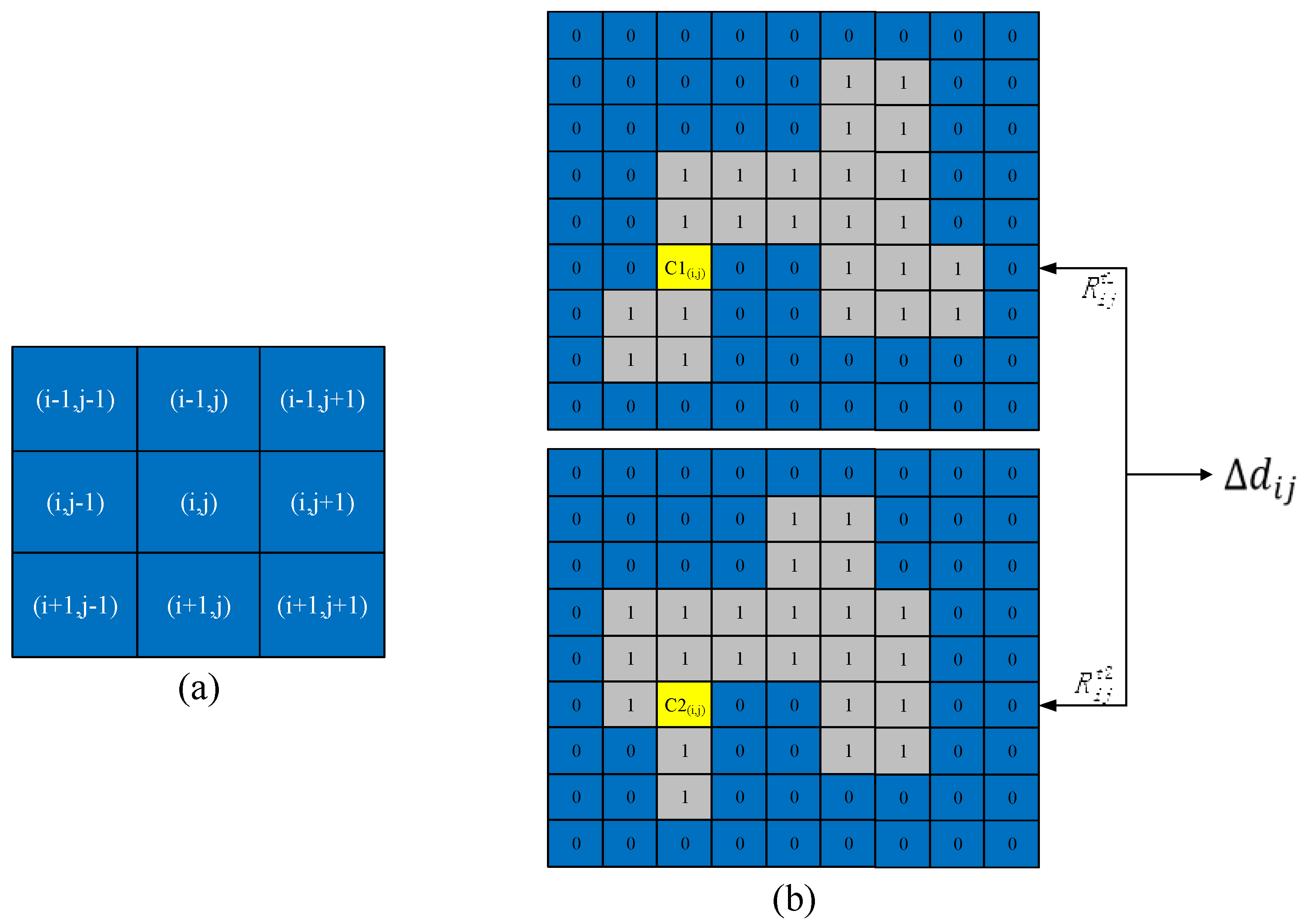
To clearly demonstrate the generation of the CMI, an extended example is shown in Figure 2. In Figure 2, where C1(i,j) and C2(i,j) are the central pixels of bi-temporal images, Figure 2a is an eight neighboring extension detector, and the pixels which are composed of adaptive extended regions are marked by “1”. In the progress of an extension, it is extended gradually from a central pixel to an adaptive extended region by using the extension detector, the spectral similarity between the central pixel and its neighboring pixels are measured to decide whether a neighboring pixel should be marked as “1” or not according to a pre-defined threshold T1. The extensions will be terminated when the size of the extended region meets the predefined threshold T2. Finally, the change magnitude between the two central pixels (C1(i,j) and C2(i,j)) is measured by the distance ( Δ d i j ) between the two adaptive extended regions, more details can be tracked in Formulas (2)–(4).
From a theoretical viewpoint, it is worth noting that advantage of the proposed strategy for generating change magnitude image lies in the following aspects: (1) since the shape and size of the extended region is adaptive, the pixels within an adaptive region give a higher similarity in spectra, it is more objective than considering the contextual information through a regular window or a mathematical model; (2) Based on the constraints of the two parameters T1 and T2, the extension of a region around a pixel is self-adaptive and the mean value of the pixels within an extended region is used to measure the change magnitude between the pairwise pixel. Hence, the proposed strategy can smooth the intra-class noise, and improve the performance of change detection.
It is well known that image difference is one of the simplest and most widely used methods for generating change magnitude image [3,4,37,45]. To illustrate the advantage of the proposed approach, the change magnitude image for a bi-temporal image is respectively acquired by image difference and the proposed approach, and the results are compared in Figure 3. The local standard deviation (std) of CMI is compared using the same window ( 40 × 40 ) which is highlighted in each sub-figure. Lower standard deviation performs a higher homogeneity of the change or unchanged area. As shown in Figure 3, the standard deviation is reduced from std = 13.83 to std = 12.76 with the T1 range from 30 to 70. Compared with Figure 3a, the standard deviation (std = 19.48) of the observed window which is based on the CMI obtained by the image difference method, the CMI of the proposed approach provides a smaller standard deviation. Therefore, it can be found that the proposed approach has an advantage in improving the homogeneity of a local area, and this improvement is beneficial for LCCD.

2.3. Threshold for Obtaining Binary Change Detection Map

As in many existing LCCD methods, a threshold is needed to determine if a pixel of CMI is changed or unchanged and to generate the binary change detection map. In the proposed approach, a most popular binary method, named Otsu [37,38,50], is used to automatically participate a change magnitude image into a binary change detection map. The Otsu approach assumes that the CMI contains two classes (change and unchanged) of pixels. It then calculates the optimum threshold dividing the two classes to minimize the intra-class variance or equivalently. In other words, the Otsu method searches exhaustively for the threshold which can minimize the variance within the changed pixel and unchanged pixels. In addition, a manual threshold is allowed to divide CMI into a binary change detection map in the proposed approach.

3. Experiment

In this section, the proposed approach was investigated by three experiments based on three images scenes which depict the different land cover change events. Three widely used contextual information-based methods, i.e., LSELUC [45], MLS [46], PCA_Kmeans [43], and CVA [36], were compared with the proposed approach in terms of performance of effectiveness.

3.1. Dataset Description

Three image datasets which depict land cover change event in the real world are used to investigate the performance of different contextual information-based LCCD methods, including the proposed approach. Details of the datasets are presented in this section as follows:
The first dataset is an open-access dataset for change detection evaluation. As shown in Figure 4, this dataset depicts a land cover change event in Mexico, which is related to a forest fire in May 2002. The images are composed of two 8-bits images acquired by Landsat-7 satellite sensor in April 2000 and May 2002. The size of the entire image scene is 512 × 512 pixels with a spatial resolution 30 m/pixel. For comparison of the bi-temporal images, it should be noted that fire destroyed a large portion of the forest in the considered change area. The reference change map was interpreted manually to obtain a quantitative evaluation, as shown in Figure 4d.
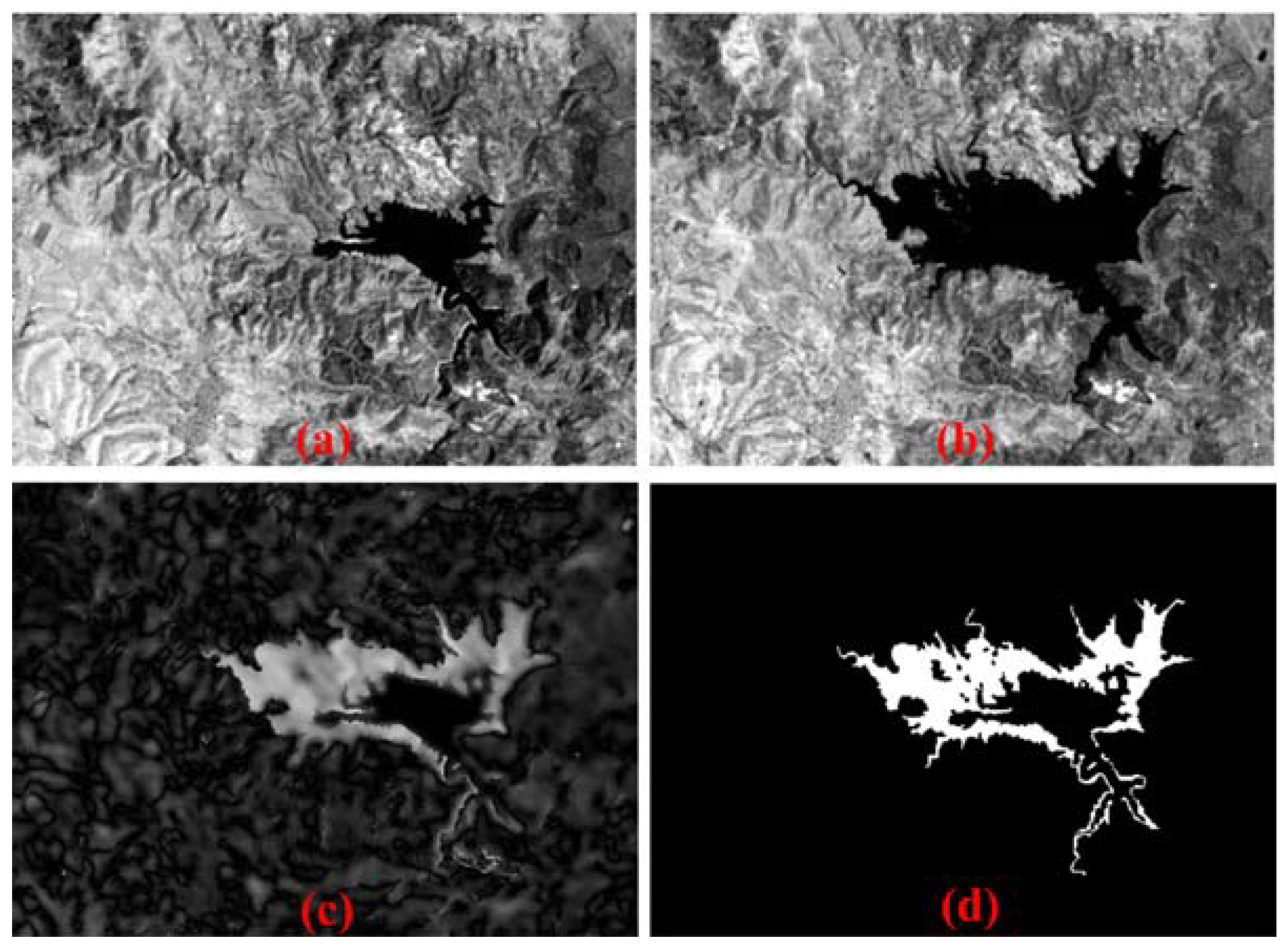
As shown in Figure 5, the second dataset is also free-access and the two images are composed of two 8-bit images acquired by Landsat-5 satellite on September 1995 and July 1996, respectively. The size of the images is 412 × 300 pixels with a spatial resolution 30 m/pixel. This dataset depicts the water lever change event of the Lake Mulargia on Sardinia Island (Italy) between the two aforementioned acquisition dates. The ground reference map is shown in Figure 5d, and it is defined manually according to the detailed visual analysis base on the bi-temporal image comparisons.
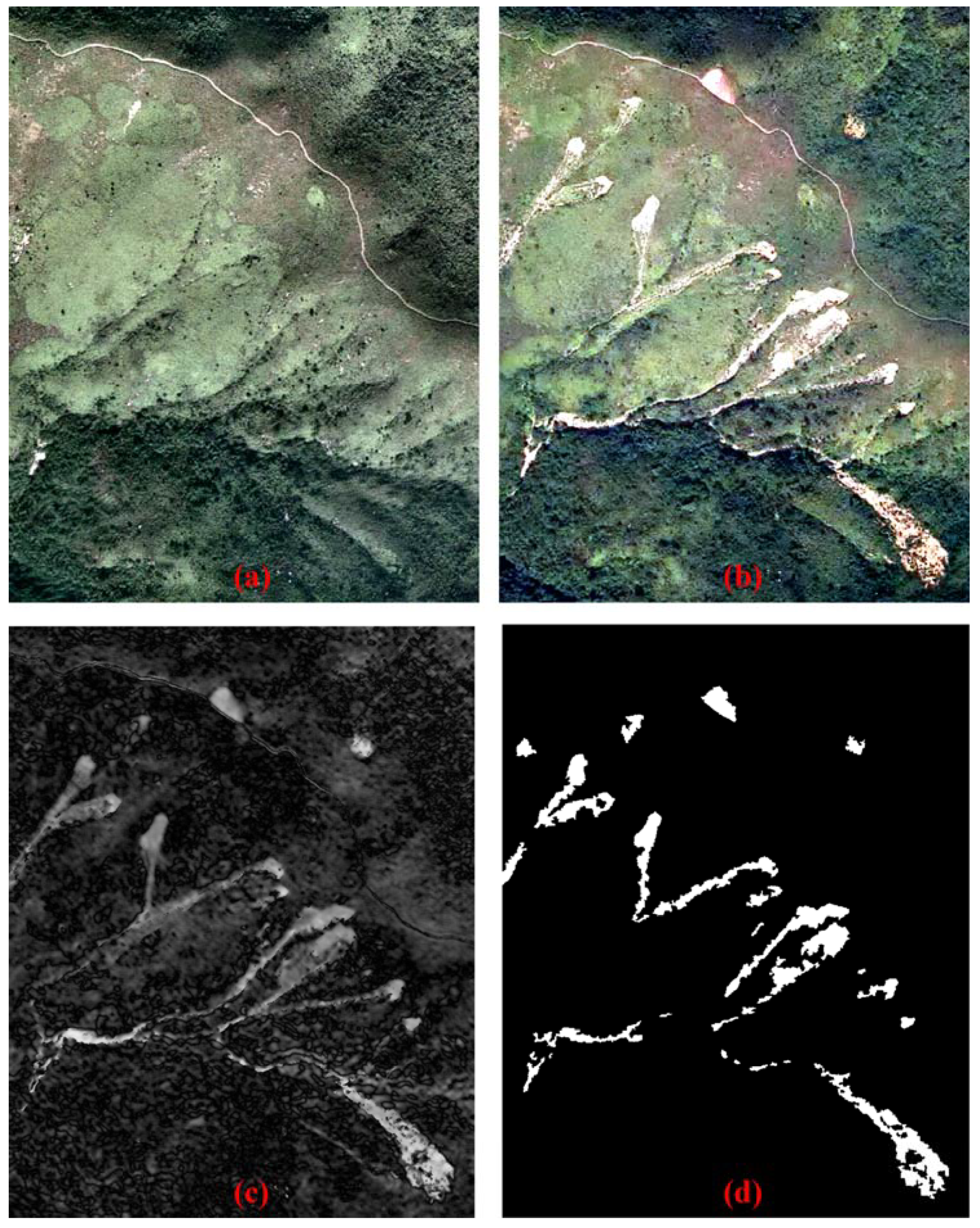
The third dataset is acquired using Zeiss RMK TOP-15 aerial survey camera from the flying height of approximately 2400 m in April 2007 and July 2014. The bi-temporal images with very high–spatial resolution of 0.5 m/pixel depict the pre-event and post-event of land sliding case in Lantau Island of Hong Kong, China. The size of each image is 750 × 950 pixels and the imagery covers a landside site, as shown in Figure 6. From the image scene, it can be found that it is a challenging task to obtain the landslide inventory map through remote sensing change detection techniques, because the area is covered by various types of forest and grasslands. Furthermore, the bi-temporal images are captured at different times with a different sun height, thereby resulting in a relatively high spectral heterogeneity, especially for the shadows of high trees.

3.2. Experimental Setup and Parameter Setting

To test the effectiveness of the proposed approach for LCCD using bi-temporal remote sensing images, three popular LCCD methods, including LSELUC [45], MLS [46], CVA [36], and PCA_Kmeans [43], were compared with the proposed approach. For each dataset, the optimal parameters of each experiment were obtained by the trial-and-error approach, the parameter details of each approach were summarized in Table 1. In addition, to present quantitative comparisons, the number of ground reference pixels for each dataset is given in Table 2.

3.3. Results and Quantitative Evaluation

Three quantitative evaluation measurements, i.e., false alarm (FA), missed alarm (MA), and total error (TE), are employed for experimental comparisons to evaluate the proposed approach quantitatively [51]. To present the meaning of these indices, we defined UC as the number of change pixels that are actually unchanged pixels in BCDM when compared with the ground reference, TRU is the number of pixels that are unchanged pixels in the ground reference, CU is the unchanged pixels in the BCDM but is changed pixels in the ground reference, TRC is the total number of changed pixels in the ground reference truth. Based on this definition, FA, MA and TE can be defined as the U C T R U × 100 % , C U T R C × 100 % , and U C   +   C U T R C   +   T R U × 100 % , respectively.
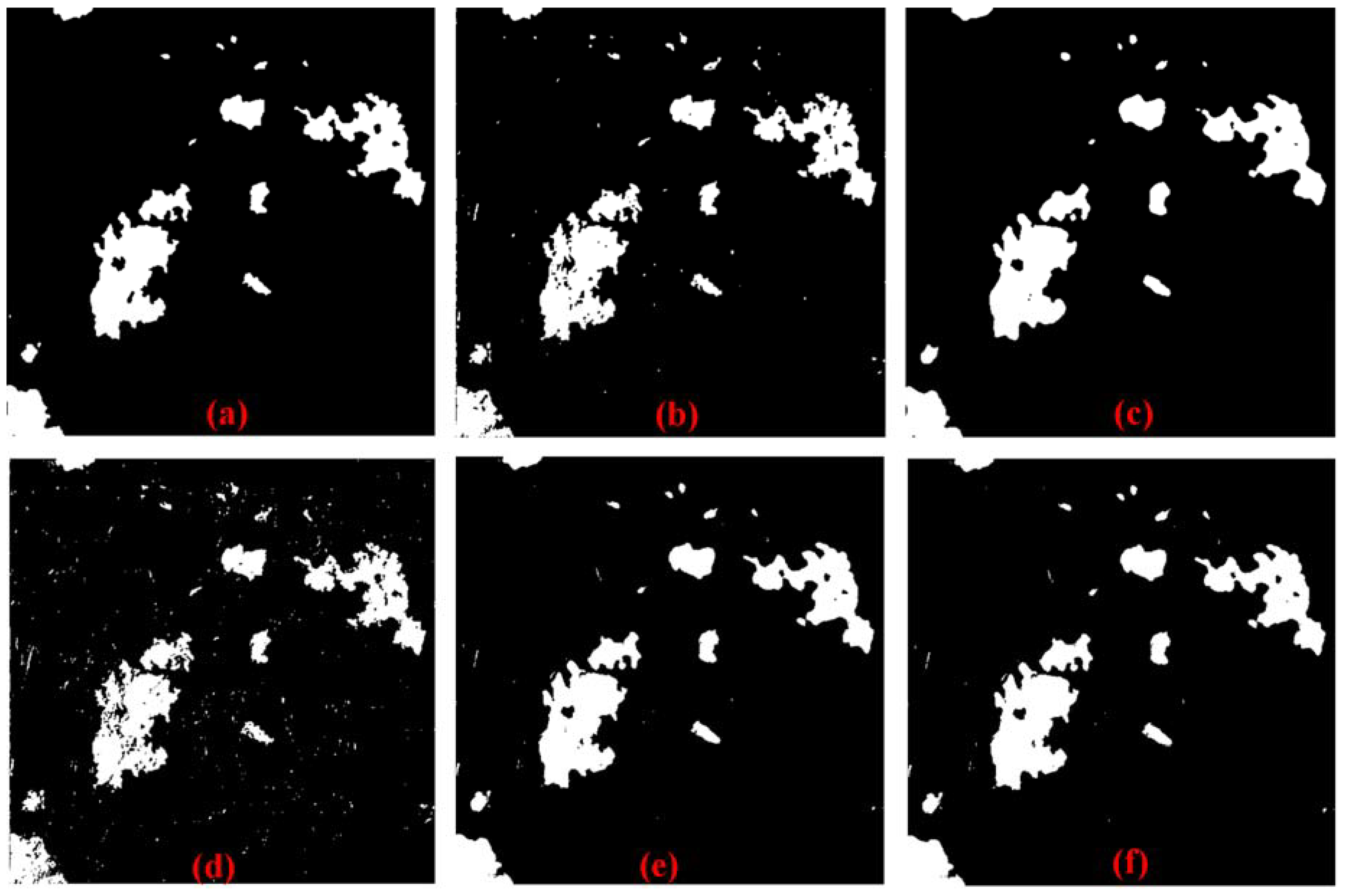
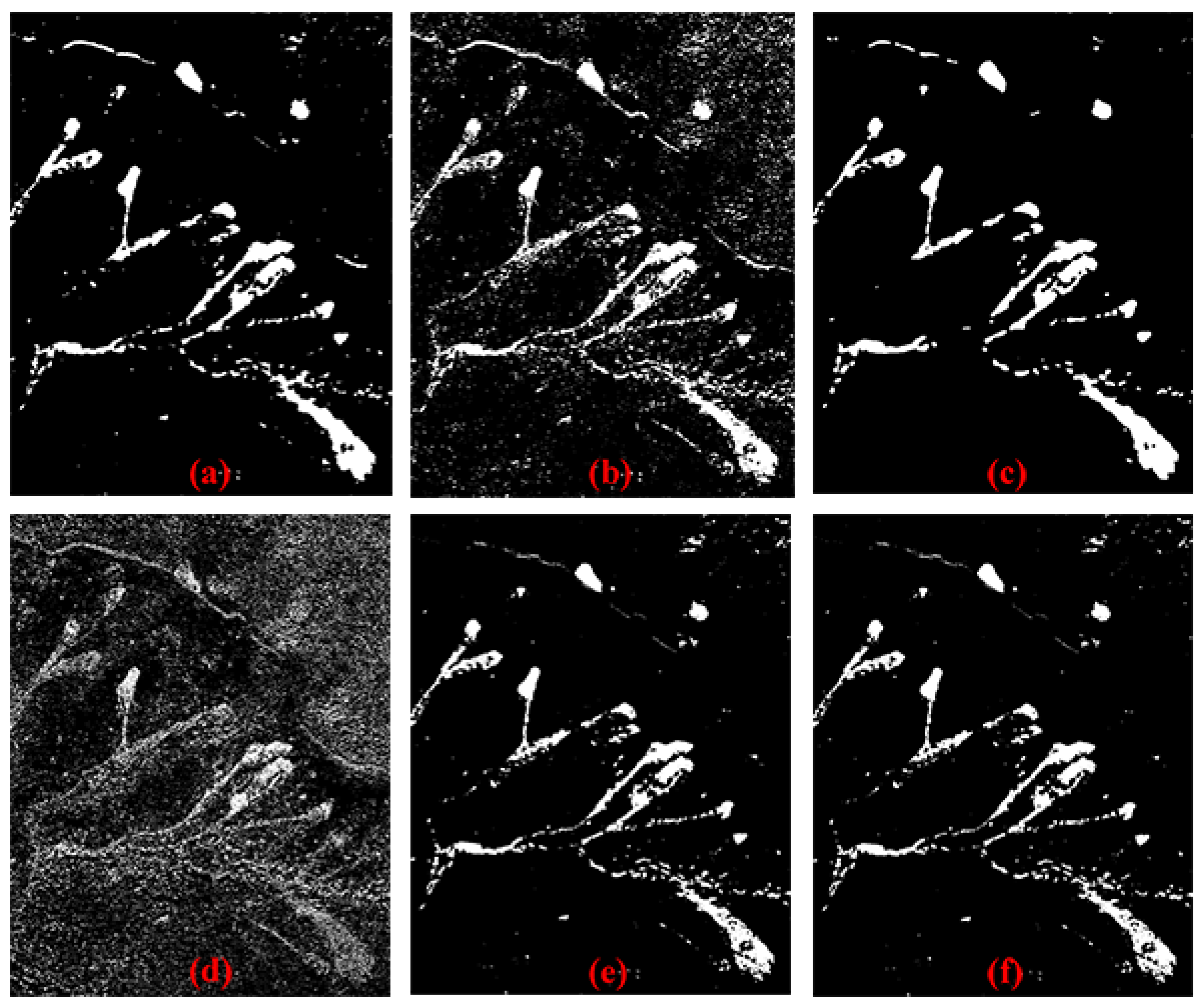
The first image scene depicts a land cover change event about a forest fire in Mexico, as illustrated in Figure 4. Visual comparisons are shown in Figure 7, from these comparisons, it clearly demonstrates that the proposed approach with Otsu or manual threshold performed better than that of LSELUC [45], MLS [46], CVA [35] and PCA_Kmeans [43]. Compared with the ground reference, the results of the proposed approach produce less noise. In addition, quantitative comparisons are presented in Table 3 where “The proposed” and “The proposed+” presented the proposed approach with Otsu binary threshold method and a manual binary threshold, respectively. It can be seen that the proposed approach achieved the best accuracies in terms of MA and TE. This comparison further demonstrates the superiority of the proposed approach.
In the second experiment, two images which cover the same geographic area, called Lake Mulargia on Sardinia Island, were adopted for experimental comparisons, as displayed in Figure 5. The results of the different methods are compared in Figure 8, from this comparisons, it can be seen that the proposed approach achieved a better performance with less noise, compared with that of LSELUC [45], MLS [46], CVA [36], and PCA_Kmeans [43]. The quantitative comparisons in Table 4 strengthen further the conclusion of the visual comparison and clearly demonstrate that the result based on the proposed approach and the proposed+ approach gave better accuracies in terms of MA and TE.
To further investigate the performance of the proposed approach, another land cover change event, i.e., landslide, was adopted to evaluate the proposed approach in a third experiment, as shown in Figure 6. The first noteworthy observations are given in Table 5. There, it can be seen that the proposed approach achieves the best accuracies for the third dataset when compared with the other methods in terms of FA and TE. For example, compared with the change detection results based on CVA [36], the improvements achieved by the proposed approach are about 12.24% and 12.81% in terms of FA and TE, respectively. The same conclusion can be drawn by the visual performance comparisons, as shown in Figure 9.

4. Discussion

From the abovementioned comparison, it can be concluded that the proposed approach is competitive compared with the LSELUC [45], MLS [46], CVA [36], and PCA_Kmeans [43] in terms of change detection accuracies and performance. To promote the application of the proposed approach in practice, we discuss two aspects of the proposed approach below.
First, we discuss the sensitivity between the parameter settings and the land cover detection accuracies. In the first experiment with the Mexico dataset, as shown in Figure 10a, when the value of T1 ranges from 5 to 75 with T2 is fixed at 50, the accuracy-MA of the proposed approach decreases initially but the accuracy of FA and TE fluctuates in a small range. However, when the value of T1 becomes larger than 75, the accuracies of MA are posed to a horizontal level. When T1 is fixed at 75 and the value of T2 varies, as shown in Figure 10b, the MA decreases from 13.5 to 9.2 with the value of T2 ranging from 5 to 50. Then, despite the value of T2 being increased larger than 50, the accuracy varies in a small range. From this discussion, it can be seen that T1 indicates the spectral difference between the central pixel and its surrounding pixels, and T2 indicates the maximum number of searched pixels around a central pixel. Furthermore, T1 and T2 complement each other, when one of the parameters is fixed, the accuracies will pose to a horizontal level, and the accuracies will not increase additionally with the increase of another parameter.
In the second experiment with the Sardinia Island dataset, the sensitivity between T1 and the detection accuracies with T2 = 50 is shown in Figure 10c. This sensitivity result clearly indicates that MA decreases gradually when the value of T1 ranges from 5 to 50. However, MA increases when the T1 is larger than 50. That is because a larger T1 will allow the consideration of more sufficient spatial neighboring information around a central pixel. However, a too large T1 may result in more heterogeneous pixels in an adaptive extended region. This is detrimental to the subsequent calculation of the change magnitude image. In addition, FA and TE gradually posed to a stable trend after T1 reaches the value of 110, as shown in Figure 10c. However, when T1 is fixed at 110, and T2 varies from 5 to 150, as shown in Figure 10d, it can be seen that MA increases with the increase of T2, but FA and TE nearly maintain a horizontal level.
Based on the above discussion of the experiments, it is seen that (1) the parameter settings of the proposed approach should be adjusted according to the different dataset, the settings of the optimal composition parameters may be different for different image scenes; and (2) the value of FA and TE is usually small and they will pose to a horizontal level while one parameter is fixed and the other varies. This is beneficial in practice for the setting of parameters setting when the proposed approach is applied.

5. Conclusions

In this work, a simple yet effective LCCD approach is proposed. The proposed approach progressively and adaptively extends a contextual region from a central pixel to a labeled pixel group which is spectrally similar and spatially contiguous. Then, the change magnitude between pairwise pixels of bi-temporal images is instead computed in the pairwise adaptive extended region. All the bi-temporal images are scanned and processed to generate a change magnitude image (CMI). Finally, an Otsu binary automatic method or manual binary threshold is employed to obtain the binary change detection result. The contribution of this study can be briefly summarized as follows:
(1)
The proposed approach provides competitive change detection results. For the two image scenes that are related to two different real land cover change events, the detection results demonstrate the effectiveness and superiority of the proposed approach in terms of visual performance and quantitatively accuracies when compared to widely used methods, such as LSELUC [45], MLS [46], CVA [36], and PCA_Kmeans [43].
(2)
To the best of our knowledge, here for the first time, adaptive region-based distance is applied instead of single pixel-based distance to measure the change magnitude between pairwise pixels of bi-temporal images. The experimental results demonstrate that this proposed approach is helpful for improving the change detection accuracies and performance. The reason for this is that the pixels are highly correlated with their neighbors in the image spatial domain, especially for a ground object (such as a meadow), and this correlation is consistent with the shape and size of an object. Therefore, the proposed contextual information around a pixel based on adaptive region can be considered objective and reasonable.
In future studies, extensive investigations of the proposed approach will be conducted with the following focus: (1) the automation of parameters of the proposed approach should be considered. If T1 and T2 can be estimated in an automatic manner, it will be helpful for improving the automation degree of the proposed approach; (2) more investigations based on different remote sensing images, such as unmanned aerial vehicle images and satellite images with very high spatial resolutions, will be conducted in order to enhance the robustness of the approach. Furthermore, extensive investigations will broaden the usability of the proposed approach.

Author Contributions

Z.L. was primarily responsible for the original idea and experimental design. T.L. and Y.C. did the experiments and provided several helpful suggestions. P.Z. provided contributions to improve the quality of the paper in the writing procedure. J.A.B. provided ideas to improve the quality of the paper.

Acknowledgments

The authors thank the editor-in-chief, associate editor, and reviewers for their insightful comments and suggestions. This work was supported by the National Science Foundation China (61701396), the Natural Science Foundation of Shaan Xi Province (2017JQ4006), Engineering Research Center of Geospatial Information and Digital Technology, NASG (SIDT20171003), The National Key Research and Development Program of China(018YFF0215006), Natural Science Foundation of Jiangsu Province, China (BK20150835), and Tibet Natural Science Foundation-The study of Tibet crop condition monitoring based on crop growth model and multi-source remote sensing data (2016-ZR-15-18).

Conflicts of Interest

The authors declare no conflict of interest.

References

  1. Coppin, P.; Jonckheere, I.; Nackaerts, K.; Muys, B.; Lambin, E. Review articledigital change detection methods in ecosystem monitoring: A review. Int. J. Remote Sens. 2004, 25, 1565–1596. [Google Scholar] [CrossRef]
  2. Radke, R.J.; Andra, S.; Al-Kofahi, O.; Roysam, B. Image change detection algorithms: A systematic survey. IEEE Trans. Image Process. 2005, 14, 294–307. [Google Scholar] [CrossRef] [PubMed]
  3. Lu, D.; Mausel, P.; Brondizio, E.; Moran, E. Change detection techniques. Int. J. Remote Sens. 2004, 25, 2365–2401. [Google Scholar] [CrossRef]
  4. Singh, A. Review article digital change detection techniques using remotely-sensed data. Int. J. Remote Sens. 1989, 10, 989–1003. [Google Scholar] [CrossRef]
  5. Dewan, A.M.; Yamaguchi, Y. Land use and land cover change in Greater Dhaka, Bangladesh: Using remote sensing to promote sustainable urbanization. Appl. Geogr. 2009, 29, 390–401. [Google Scholar] [CrossRef]
  6. Truong, C.; Oudre, L.; Vayatis, N. A review of change point detection methods. arXiv, 2018; arXiv:1801.00718. [Google Scholar]
  7. Zhu, Z. Change detection using landsat time series: A review of frequencies, preprocessing, algorithms, and applications. ISPRS J. Photogramm. Remote Sens. 2017, 130, 370–384. [Google Scholar] [CrossRef]
  8. Tewkesbury, A.P.; Comber, A.J.; Tate, N.J.; Lamb, A.; Fisher, P.F. A critical synthesis of remotely sensed optical image change detection techniques. Remote Sens. Environ. 2015, 160, 1–14. [Google Scholar] [CrossRef] [Green Version]
  9. Xiao, J.; Shen, Y.; Ge, J.; Tateishi, R.; Tang, C.; Liang, Y.; Huang, Z. Evaluating urban expansion and land use change in Shijiazhuang, China, by using GIS and remote sensing. Landsc. Urban Plan. 2006, 75, 69–80. [Google Scholar] [CrossRef]
  10. Shahraki, S.Z.; Sauri, D.; Serra, P.; Modugno, S.; Seifolddini, F.; Pourahmad, A. Urban sprawl pattern and land-use change detection in Yazd, Iran. Habitat Int. 2011, 35, 521–528. [Google Scholar] [CrossRef]
  11. Weng, Q.; Lu, D.; Schubring, J. Estimation of land surface temperature-vegetation abundance relationship for urban heat island studies. Remote Sens. Environ. 2004, 89, 467–483. [Google Scholar] [CrossRef]
  12. Lo, C.; Quattrochi, D.A. Land-use and land-cover change, urban heat island phenomenon, and health implications. Photogramm. Eng. Remote Sens. 2003, 69, 1053–1063. [Google Scholar] [CrossRef]
  13. Sun, L.; Wei, J.; Duan, D.; Guo, Y.; Yang, D.; Jia, C.; Mi, X. Impact of land-use and land-cover change on urban air quality in representative cities of china. J. Atmos. Sol.-Terr. Phys. 2016, 142, 43–54. [Google Scholar] [CrossRef]
  14. Moody, D.I. Change Detection and Change Monitoring of Natural and Man-Made Features in Multispectral and Hyperspectral Satellite Imagery. U.S. Patent No. 9,946,931, 17 April 2018. [Google Scholar]
  15. McDonnell, M.J.; Hahs, A.K. The use of gradient analysis studies in advancing our understanding of the ecology of urbanizing landscapes: Current status and future directions. Landsc. Ecol. 2008, 23, 1143–1155. [Google Scholar] [CrossRef]
  16. Modica, G.; Vizzari, M.; Pollino, M.; Fichera, C.; Zoccali, P.; Di Fazio, S. Spatio-temporal analysis of the urban–rural gradient structure: An application in a mediterranean mountainous landscape (Serra San Bruno, Italy). Earth Syst. Dyn. 2012, 3, 263–279. [Google Scholar] [CrossRef]
  17. Yang, Y.; Zhou, Q.; Gong, J.; Wang, Y. Gradient analysis of landscape spatial and temporal pattern changes in Beijing metropolitan area. Sci. China Technol. Sci. 2010, 53, 91–98. [Google Scholar] [CrossRef]
  18. Desclée, B.; Bogaert, P.; Defourny, P. Forest change detection by statistical object-based method. Remote Sens. Environ. 2006, 102, 1–11. [Google Scholar] [CrossRef]
  19. Hermosilla, T.; Wulder, M.A.; White, J.C.; Coops, N.C.; Hobart, G.W. Regional detection, characterization, and attribution of annual forest change from 1984 to 2012 using landsat-derived time-series metrics. Remote Sens. Environ. 2015, 170, 121–132. [Google Scholar] [CrossRef]
  20. El-Kawy, O.A.; Rød, J.; Ismail, H.; Suliman, A. Land use and land cover change detection in the western Nile delta of Egypt using remote sensing data. Appl. Geogr. 2011, 31, 483–494. [Google Scholar] [CrossRef]
  21. Prakasam, C. Land use and land cover change detection through remote sensing approach: A case study of Kodaikanal taluk, Tamil nadu. Int. J. Geomat. Geosci. 2010, 1, 150. [Google Scholar]
  22. Fichera, C.R.; Modica, G.; Pollino, M. GIS and remote sensing to study urban-rural transformation during a fifty-year period. In International Conference on Computational Science and Its Applications; Springer: Berlin/Heidelberg, Germany, 2011; pp. 237–252. [Google Scholar]
  23. Jin, S.; Yang, L.; Zhu, Z.; Homer, C. A land cover change detection and classification protocol for updating Alaska NLCD 2001 to 2011. Remote Sens. Environ. 2017, 195, 44–55. [Google Scholar] [CrossRef]
  24. Jin, S.; Yang, L.; Danielson, P.; Homer, C.; Fry, J.; Xian, G. A comprehensive change detection method for updating the national land cover database to circa 2011. Remote Sens. Environ. 2013, 132, 159–175. [Google Scholar] [CrossRef]
  25. Zhu, Z.; Woodcock, C.E. Continuous change detection and classification of land cover using all available landsat data. Remote Sens. Environ. 2014, 144, 152–171. [Google Scholar] [CrossRef]
  26. Zhang, P.; Lv, Z.; Shi, W. Local spectrum-trend similarity approach for detecting land-cover change by using spot-5 satellite images. IEEE Geosci. Remote Sens. Lett. 2014, 11, 738–742. [Google Scholar] [CrossRef]
  27. Lv, Z.; Liu, T.; Wan, Y.; Benediktsson, J.A.; Zhang, X. Post-processing approach for refining raw land cover change detection of very high-resolution remote sensing images. Remote Sens. 2018, 10, 472. [Google Scholar] [CrossRef]
  28. Wu, T.; Luo, J.; Fang, J.; Ma, J.; Song, X. Unsupervised object-based change detection via a Weibull mixture model-based binarization for high-resolution remote sensing images. IEEE Geosci. Remote Sens. Lett. 2018, 15, 63–67. [Google Scholar] [CrossRef]
  29. Bruzzone, L.; Prieto, D.F. Automatic analysis of the difference image for unsupervised change detection. IEEE Trans. Geosci. Remote Sens. 2000, 38, 1171–1182. [Google Scholar] [CrossRef]
  30. Zanetti, M.; Bruzzone, L. A theoretical framework for change detection based on a compound multiclass statistical model of the difference image. IEEE Trans. Geosci. Remote Sens. 2018, 56, 1129–1143. [Google Scholar] [CrossRef]
  31. Xu, L.; Zhang, S.; He, Z.; Guo, Y. The comparative study of three methods of remote sensing image change detection. In Proceedings of the 17th International Conference on IEEE Geoinformatics, Fairfax, VA, USA, 12–14 August 2009; pp. 1–4. [Google Scholar]
  32. Lu, D.; Mausel, P.; Batistella, M.; Moran, E. Land-cover binary change detection methods for use in the moist tropical region of the amazon: A comparative study. Int. J. Remote Sens. 2005, 26, 101–114. [Google Scholar] [CrossRef]
  33. Malila, W.A. Change vector analysis: An approach for detecting forest changes with landsat. In Proceedings of the LARS Symposia, 1980; page number: 385. Available online: https://docs.lib.purdue.edu/cgi/viewcontent.cgi?article=1386&context=lars_symp (accessed on 6 June 2018).
  34. Bovolo, F.; Bruzzone, L. A theoretical framework for unsupervised change detection based on change vector analysis in the polar domain. IEEE Trans. Geosci. Remote Sens. 2007, 45, 218–236. [Google Scholar] [CrossRef]
  35. Chen, Q.; Chen, Y. Multi-feature object-based change detection using self-adaptive weight change vector analysis. Remote Sens. 2016, 8, 549. [Google Scholar] [CrossRef]
  36. Xiaolu, S.; Bo, C. Change detection using change vector analysis from landsat tm images in Wuhan. Procedia Environ. Sci. 2011, 11, 238–244. [Google Scholar] [CrossRef]
  37. Lv, Z.; Shi, W.; Zhou, X.; Benediktsson, J.A. Semi-automatic system for land cover change detection using Bi-temporal remote sensing images. Remote Sens. 2017, 9, 1112. [Google Scholar] [CrossRef]
  38. Otsu, N. A threshold selection method from gray-level histograms. IEEE Trans. Syst. Man Cybern. 1979, 9, 62–66. [Google Scholar] [CrossRef]
  39. Hao, M.; Shi, W.; Zhang, H.; Li, C. Unsupervised change detection with expectation-maximization-based level set. IEEE Geosci. Remote Sens. Lett. 2014, 11, 210–214. [Google Scholar] [CrossRef]
  40. Celik, T. A bayesian approach to unsupervised multiscale change detection in synthetic aperture radar images. Signal Process. 2010, 90, 1471–1485. [Google Scholar] [CrossRef]
  41. Celik, T. Change detection in satellite images using a genetic algorithm approach. IEEE Geosci. Remote Sens. Lett. 2010, 7, 386–390. [Google Scholar] [CrossRef]
  42. Ng, H.-F. Automatic thresholding for defect detection. Pattern Recognit. Lett. 2006, 27, 1644–1649. [Google Scholar] [CrossRef]
  43. Celik, T. Unsupervised change detection in satellite images using principal component analysis and k-means clustering. IEEE Geosci. Remote Sens. Lett. 2009, 6, 772–776. [Google Scholar] [CrossRef]
  44. Lv, Z.; Zhang, W. Contextual analysis based approach for detecting change from high resolution satellite imagery. J. Indian Soc. Remote Sens. 2018, 46, 43–50. [Google Scholar] [CrossRef]
  45. Zhang, X.; Shi, W.; Liang, P.; Hao, M. Level set evolution with local uncertainty constraints for unsupervised change detection. Remote Sens. Lett. 2017, 8, 811–820. [Google Scholar] [CrossRef]
  46. Bazi, Y.; Melgani, F.; Al-Sharari, H.D. Unsupervised change detection in multispectral remotely sensed imagery with level set methods. IEEE Trans. Geosci. Remote Sens. 2010, 48, 3178–3187. [Google Scholar] [CrossRef]
  47. Lv, Z.; Shi, W.; Benediktsson, J.A.; Gao, L. A modified mean filter for improving the classification performance of very high-resolution remote-sensing imagery. Int. J. Remote Sens. 2018, 39, 770–785. [Google Scholar]
  48. Lv, Z.; Zhang, P.; Atli Benediktsson, J. Automatic object-oriented, spectral-spatial feature extraction driven by tobler’s first law of geography for very high resolution aerial imagery classification. Remote Sens. 2017, 9, 285. [Google Scholar] [CrossRef]
  49. Huang, X.; Zhang, L.; Li, P. An adaptive multiscale information fusion approach for feature extraction and classification of IKONOS multispectral imagery over urban areas. IEEE Geosci. Remote Sens. Lett. 2007, 4, 654–658. [Google Scholar] [CrossRef]
  50. Gong, M.; Zhou, Z.; Ma, J. Change detection in synthetic aperture radar images based on image fusion and fuzzy clustering. IEEE Trans. Image Process. 2012, 21, 2141–2151. [Google Scholar] [CrossRef] [PubMed]
  51. Yetgin, Z. Unsupervised change detection of satellite images using local gradual descent. IEEE Trans. Geosci. Remote Sens. 2012, 50, 1919–1929. [Google Scholar] [CrossRef]
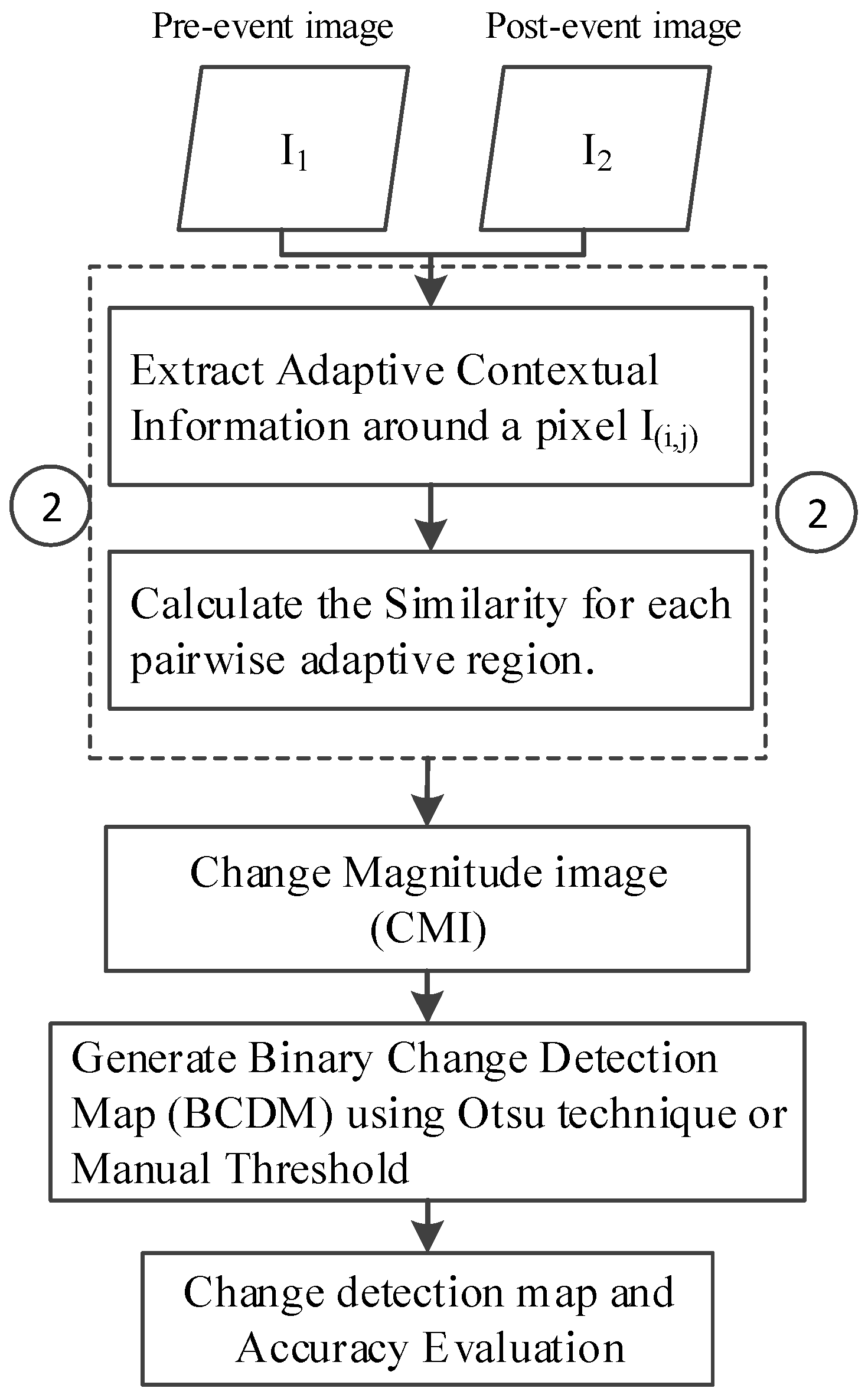
Figure 1. Flowchart of the proposed approach.
Remotesensing 10 00901 g001
Figure 2. Examples of Adaptive Extended Regions: (a) An eight neighboring extension detector, and (b) the two regions labeled by “1” are the adaptive extended regions surrounding the central pixel C1(i,j) and C2(i,j), respectively.
Remotesensing 10 00901 g002
Figure 3. Change Magnitude Image Comparisons between the Image Difference and The Proposed Approach: (a) is the CMI obtained by image difference method; (bf) are the CMIs obtained by the proposed approach with a fixed T2 = 50. T1 is equal to 30, 40, 50, 60, and 70 for each sub-figure from (b) to (f), respectively.
Remotesensing 10 00901 g003
Figure 4. Images of Mexico Area: (a) band 4 of the Landsat ETM+ captured in April 2000, (b) band 4 of the Landsat ETM+ captured in May 2002, (c) corresponding CMI obtained by the proposed approach, and (d) reference map of the changed area.
Remotesensing 10 00901 g004
Figure 5. Image of Sardinia Island area in Italy: (a) band 4 of the Landsat TM image captured in September 1995, (b) band 4 of the Landsat TM image captured in July 1996, (c) corresponding CMI based on the proposed approach, and (d) reference map of the changed area.
Remotesensing 10 00901 g005
Figure 6. Image of landslide area in Lantau Island, Hong Kong, China: (a) pre-event image captured in April 2007, (b) post-event image captured in July 2014, (c) corresponding CMI based on the proposed approach, and (d) reference map of the changed area.
Remotesensing 10 00901 g006
Figure 7. Mexico dataset: Binary change detection map generated by different methods: (a) LSELUC [45]; (b) MLS [46]; (c) PCA_Kmeans [43]; (d) CVA [36]; (e,f) the proposed approach with Otsu binary threshold and manual threshold, respectively.
Remotesensing 10 00901 g007
Figure 8. Sardinia Island dataset: Binary change detection map generated by different methods: (a) LSELUC [45]; (b) MLS [46]; (c) PCA_Kmeans [43]; (d) CVA [36]; (e,f) the proposed approach with Otsu binary threshold and manual threshold, respectively.
Remotesensing 10 00901 g008
Figure 9. Landslide on Landtau Island dataset: Binary change detection map generated by different methods: (a) LSELUC [45]; (b) MLS [46]; (c) PCA_Kmeans [43]; (d) CVA [36]; (e,f) the proposed approach with the Otsu binary threshold and a manual threshold, respectively.
Remotesensing 10 00901 g009
Figure 10. Relationship between detection accuracy and setting of parameters (T1 and T2) for the proposed approach with Otsu binary threshold in each experiment: (a,b) give the relationship between T1, T2 for the Mexico dataset, respectively; (c,d) gives the relationship between T1, T2 for the Sardinia Island dataset, respectively.
Remotesensing 10 00901 g010
Table 1. Parameter settings of different LCCD methods for the three datasets.
MethodParameter Settings
Mexico DatasetSardinia DatasetHong Kong Dataset
LSELUC [45]S = 7S = 3S = 9
MLS [46]L = 2, μ = 0.1L = 2, μ   = 0.3L = 2, μ   = 0.3
PCA_Kmeans [43]h = 9, s = 3h = 5, s = 3h = 9, s = 5
CVA [36]T = 46T = 67T = 109
The proposedT1 = 75, T2 = 50T1 = 110, T2 = 50T1 = 135, T2 = 50
Table 2. Details of ground reference pixels for each dataset.
Data SetPixel’s Number of Ground Reference for Each Data Set
No. of Unchanged PixelsNo. of Changed Pixels
1Mexico236,55525,589
2Sardinia115,9747626
3Hong Kong677,43435,066
Table 3. Comparison between other methods and the proposed approach for the Mexico dataset.
MethodFAMATE
LSELUC0.42612.21.58
MLS0.57811.91.68
PCA_Kmeans0.78110.31.71
CVA0.99612.62.13
The proposed0.7469.181.57
The proposed+0.7908.471.54
Table 4. Comparison between other methods and the proposed approach for the Sardinia data.
MethodFAMATE
LSELUC1.4210.11.96
MLS2.48.562.78
PCA_Kmeans1.1512.21.83
CVA3.1612.33.72
The proposed0.99513.31.76
The proposed+1.1212.31.81
Table 5. Comparison between other methods and the proposed approach for the landslide of Hong Kong dataset.
MethodFAMATE
LSELUC2.3415.73.00
MLS6.5316.47.02
PCA_Kmeans2.0818.72.90
CVA14.244.915.7
The proposed1.9620.92.89
The proposed+1.8321.72.81