A Conservative Downscaling of Satellite-Detected Chemical Compositions: NO₂ Column Densities of OMI, GOME-2, and CMAQ

Abstract

A conservative downscaling technique was applied when comparing nitrogen dioxide (NO₂) column densities from space-borne observations and a fine-scale regional model. The conservative downscaling was designed to enhance the spatial resolution of satellite measurements by applying the fine-scale spatial structure from the model, with strict mass conservation at each satellite footprint pixel level. With the downscaling approach, NO₂ column densities from the Ozone Monitoring Instrument (OMI; 13 × 24 km nadir footprint resolution) and the Global Ozone Monitoring Experiment-2 (GOME-2; 40 × 80 km) show excellent agreement with the Community Multiscale Air Quality (CMAQ; 4 × 4 km) NO₂ column densities, with R = 0.96 for OMI and R = 0.97 for GOME-2. We further introduce an approach to reconstruct surface NO₂ concentrations by combining satellite column densities and simulated surface-to-column ratios from the model. Compared with the Environmental Protection Agency’s (EPA) Air Quality System (AQS) surface observations, the reconstructed surface concentrations show a good agreement; R = 0.86 for both OMI and GOME-2. This study demonstrates that the conservative downscaling approach is a useful tool to compare coarse-scale satellites with fine-scale models or observations in urban areas for air quality and emissions studies. The reconstructed fine-scale surface concentration field could be used for future epidemiology and urbanization studies.

1. Introduction

The continuous monitoring of tropospheric nitrogen dioxide (NO₂) is of great importance because it is one of the major pollutants that affects both humans and the biosphere directly and indirectly [1,2], and it plays an important role in tropospheric chemistry. Tropospheric NO₂ is one of six pollutants regulated by the US Environmental Protection Agency’s (EPA) National Ambient Air Quality Standards, with the criteria set at 100 ppb for 1 h and 53 ppb for the annual average, according to the Clean Air Act (https://www.epa.gov/criteria-air-pollutants/naaqs-table). NO₂ is also a primary precursor for ozone formation, in association with nitrogen oxides (NO_x = NO + NO₂) and volatile organic compounds (e.g., [3,4]) and serves as an absorber of solar radiation, which affects the radiation budget [5]. Further, NO₂ is also an important indicator for traffic and urbanization [6,7,8], as estimated via NO_x emissions.

Since the launch of the Global Ozone Monitoring Experiment (GOME) in 1995 [9], NO₂ column density measurements from satellites have proven to be effective at complementing sparse surface NO₂ monitoring sites in order to provide global coverage. Four instruments have been used to monitor tropospheric NO₂ column densities from satellites, with varying resolution and overpass time. The GOME (1996–2003, onboard the European Remote Sensing-2), Scanning Imaging Absorption SpectroMeter for Atmospheric CHartographY (SCIAMACHY) (2002–2012, onboard ENVISAT), Ozone Monitoring Instrument (OMI) (2004-present, onboard Aura), and GOME-2 (2007-present, onboard MetOp-A and MetOp-B) have all been used for the detection of NO_x emission sources, the analysis of multi-year trends, and the evaluation of emission inventories [10,11,12,13,14,15,16,17,18,19,20].

While NO_x emissions come from both natural and anthropogenic sources, the dominant portion is anthropogenic, mostly from road vehicles and point sources such as energy and industrial productions, where high temperature combustions are required. The NO₂ plumes from urban anthropogenic sources usually have a high spatial gradient, which cannot be easily detected with currently operating satellite observations. Kim et al. [21] demonstrated that this geometric resolution issue itself can cause a systematic bias of more than 100% at urban locations, in addition to existing uncertainties from stratosphere-troposphere separation, air mass factors, priori NO₂ model (e.g., vertical profile and/or model surface type resolution), upper tropospheric NO₂ (e.g., lightning NO_x), and diurnal variation in NO₂ column densities [22,23,24,25].

The spatial inhomogeneity of urban NO₂ plumes becomes a practical problem as the focus of satellite data analysis moves from global distribution to regional- or local-scale urban plumes. The need for fine-scale modeling, smaller than the scale of satellite footprint pixels, is required now. The goal of this study is to compare two satellite-retrieved products of varying spatial resolutions with modeling results. We adopt the conservative downscaling technique developed by Kim et al. [21] to compare OMI (13 × 24 km nadir footprint resolution) and GOME-2 (with 40 × 80 km) NO₂ column densities with Community Multiscale Air Quality (CMAQ)-simulated NO₂ column densities in 4 km by 4 km grid spacing.

The remainder of the paper is organized as follows. In Section 2 we provide basic information on NO₂ column data from OMI and GOME-2 and describe the CMAQ simulation configuration and its emission inputs. Section 3 presents the two spatial regridding methods used, namely, “conservative regridding” and “conservative downscaling.” Section 4 elaborates on the results, discusses the differences between the two satellite NO₂ column observations, and compares them with modeled NO₂ column densities. A reconstruction of the surface NO₂ concentration field based on the downscaled NO₂ column densities, along with a comparison of the surface observations, will be demonstrated in Section 5. Finally, Section 6 concludes the paper.

2. Data and Model

2.1. Study Domain

Southern California, which includes highly populated urban (e.g., Los Angeles) and suburban- to rural- areas, was selected as the study domain. Figure 1 shows the geographical coverage of the study, focusing on greater Los Angeles, its neighboring cities (e.g., San Diego, Riverside, Bakersfield, Santa Barbara, and Mexicali), the surrounding mountains, and the ocean off the coast of the basin. The domain spans 652 km and 460 km in the east–west and north–south directions, respectively. Colored circles represent the annual mean surface of NO₂ concentrations in 2008 from the EPA’s Air Quality System (AQS) surface monitoring sites, showing high NO₂ concentrations near urban cores. The background is the blue marble image from NASA’s worldview website (https://worldview.earthdata.nasa.gov/).

2.2. Model Descriptions

The Weather Research and Forecasting model (WRF) [26] version 3.4.1 was employed to provide meteorological fields to CMAQ. The WRF simulations were conducted with three nested domains, of which the grid resolutions were 36, 12, and 4 km. The model employed 30 layers vertically, with the lowest computational layer being approximately 18 m above ground level and the top at 50 hPa. The initial guess field and lateral boundary values for the outermost domain were compiled from the North American Model (NAM) [27]. Four-dimensional data assimilation was conducted using vertical soundings and surface measurements. The Yonsei University (YSU) planetary boundary layer scheme [28], WRF Single-Moment (WSM) 3-class simple ice scheme [29], rapid radiation transfer model longwave [30], Dudhia shortwave radiation [31], and Kain-Fritsch cumulus parameterization [32] were chosen for simulations after carefully considering various available options of the WRF [33].

CMAQ was configured with the SAPRC99 mechanism [34], Euler Backward Iterative chemical solver, Aero5 aerosol module, Piecewise Parabolic Method advection scheme in both the horizontal and the vertical directions, multi-scale horizontal diffusion, and Asymmetric Convective Model version-2 vertical diffusion scheme [35]. A CMAQ-ready emissions inventory was developed using various numerical tools. On-road and off-road mobile sources were estimated using the Emission Factors model (EMFAC) 2011 and the off-road model from the California Air Resources Board, respectively. Biogenic emissions were calculated using the Model of Emissions of Gases and Aerosols from Nature (MEGAN). The above aggregated emissions were then allocated to spatial and temporal grids using the Emissions Processing System (EPS). Details of the emission process are available in SCAQMD [33].

2.3. GOME-2 and OMI NO₂ Column Densities

GOME-2 and OMI tropospheric NO₂ column density data for 2008, retrieved by the Royal Netherlands Meteorological Institute (KNMI), are used in this study. The GOME-2 sensor, onboard the EUMETSAT MetOp-A satellite, takes nadir measurements at approximately 09:30 a.m. local time with footprints of 40 × 80 km² at the nadir. By contrast, OMI, onboard NASA’s Earth Observing System Aura satellite, has a local overpass time of 13:30 p.m. with a 13 × 24 km² footprint pixel resolution. Data are downloaded from the European Space Agency’s (ESA) Tropospheric Emission Monitoring Internet Service (TEMIS; http://www.temis.nl/airpollution/no2.html). TM4NO2A version 2.3 data are used for GOME-2, and DOMINO version 2.0 data are used for OMI. The Differential Optical Absorption Spectroscopy (DOAS) technique was used for both products. Details on the NO₂ column retrieval algorithms and error analysis are described in Boersma et al. [17,36]. The quality of the data is assured by discarding pixels with high cloud fraction (>40%) and contaminated by row anomaly issue. The method used for data processing is described in Section 3.

2.4. Surface Monitoring

Surface NO₂ concentration data are obtained from the EPA’s AQS data (http://www.epa.gov/ttn/airs/airsaqs/). It should be noted that most of the AQS surface NO₂ measurements are from chemiluminescence monitors with a molybdenum converter, which often overestimates NO₂ concentration owing to the interference from other reactive nitrogen species (NO_z) [37,38]. Bechle et al. [39] also reported that the NO_z interference is lower near major sources in southern California. In this study, we did not correct any potential bias caused by the interference.

3. Methodology

Sampling of the data is an essential issue in spatial regridding, which is commonly performed in satellite data processing to convert spatial resolution and map projection from a given configuration to another. Among numerous spatial regridding methods, interpolation and pixel aggregation are two of the most common. Interpolation is preferred when the target domain resolution is finer than the raw data pixels, whereas pixel aggregation is preferred for averaging all the pixels inside each domain cell when the target grid cell size is larger than the raw data pixel size.

Despite the fact that the two methods are widely utilized, the need for a more mathematically complete method for spatial regridding has been raised, especially when finer resolution is needed and/or where the conservation of measured quantity is required. Emission data are one example where mass conservation is critical to avoid spurious loss or gain. The EPA’s spatial allocator used in its Sparse Matrix Operator Kernel Emissions (SMOKE) [40] processing is one way of handling emission data without compromising mass conservation. It calculates the fractional areas of overlapping polygons between raw data pixels (e.g., county shapes) and modeling grid cells. To build a lossless spatial regridding tool, we used polygon clipping algorithms and developed a tool to perform the accurate spatial regridding of satellite data. This section introduces the two core algorithms for regridding, “conservative regridding” and “conservative downscaling”, and describes their applications using satellite data.

3.1. Conservative Regridding

The conservative regridding method reconstructs raw data pixels (e.g., satellite data) into a target domain grid cell by calculating the fractional coverage of raw data pixels within the target grid cell. Figure 2 shows an example of the conservative regridding method. The concentration of grid cell C_j can be calculated as (P₁·f₁ + P₂·f₂ + P₃·f₃ + P₄·f₄)/(f₁ + f₂ + f₃ + f₄). In general, if the raw pixel data are in the density unit (e.g., concentration), one can calculate the overlapping fractions for each data pixel and grid cell and thus calculate the grid cell concentration as a weighted average of data pixels and fractions:

$$f_{i,j}=\frac{Area\left(P_i\cap C_j\right)}{Area\left(C_j\right)}$$

(1)

$$C_j=\frac{\sum P_i·f_{i,j}}{\sum f_{i,j}}$$

(2)

where i and j are the indices of data pixel, P, and grid cell, C, $f_{i,j}$ is the overlapping fractions, and $\sum f_{i,j}$ = 1 if no missing pixels are involved in grid cell $C_j$.

This conservative regridding method is a similar approach to the variable-pixel linear reconstruction algorithm used in the astronomy community, which was developed to preserve photometry and resolution for the Hubble Space Telescope [41]. We used subroutines from the Cube Builder for IRS Spectra Maps (CUBISM) [42] based on the Sutherland–Hodgman polygon clipping algorithm [43] for the efficient calculation of overlapped fractions. More details are available in the documentation of the development of the IDL-based Geospatial Data Processor (IGDP) [44].

3.2. Conservative Downscaling

The conservative downscaling method conducts a downscaling on top of the conservative regridding. We follow the concept of meteorological downscaling, which is a common practice in regional-scale modeling to build boundary conditions from global model output. This approach needs to be distinguished from a simple approach to increase resolution. The meteorological downscaling constrains the boundary condition and allows fine-scale restructuring with its own set of physical and thermal balances. On the contrary, this approach preserves the original coarse pixel quantity from the satellite and reconstructs fine-scale structures inside each satellite pixel coverage.

Figure 3 shows an example of the conservative downscaling method using NO₂ column data from GOME-2 and OMI. GOME-2 and OMI NO₂ column data have different spatial resolutions and overpass times, which complicates the direct comparison of these two data sets. Because their spatial resolutions are vastly different (GOME-2 with 80 × 40 km² and OMI with 13 × 24 km²), the simple regridding method cannot be used in the comparison. If the normal regridding method were applied, the GOME-2 data with coarse resolution would be unable to provide spatial variations between urban source and rural receptor areas. This would result in a lower concentration in near emission sources such as downtown urban and dense road networks, and a higher concentration in suburban or rural areas, compared with the finer resolution OMI or in situ observations.

To lessen this systematic bias due to the discrepancies in spatial resolution and possibly provide a fair platform to compare various datasets with different resolution, we evaluated the use of high-resolution modeling data. As presented in Figure 3B, a CMAQ simulation was performed in the study area with 4-km resolution. Figure 3A shows the raw data pixels from the GOME-2 NO₂ column measurement (usually with 80 × 40 km² or coarser) for the southern California region on 18 August 2008. The predominantly smooth pattern in the Los Angeles region indicates the enhanced NO₂ column data. However, the 4-km CMAQ-simulated NO₂ column data at the corresponding local time (09:30 a.m.) show much more detailed spatial distributions, similar to the sources of NO_x emissions.

For each GOME-2 pixel, we retrieved collocated CMAQ pixels as shown in Figure 3B. With the usual GOME-2 pixel size and CMAQ grid cell size, around 200 cells are available per GOME-2 data pixel. A spatial weighting kernel was constructed next, as a fractional distribution of the CMAQ NO₂ concentration corresponding to a GOME-2 pixel. Selected CMAQ NO₂ concentrations were normalized (i.e., divided by the average of all selected concentrations, Figure 3C) and were then applied to the GOME-2 data pixel to reconstruct its spatial distribution as follows:

$$C_j=\frac{\sum P_i·k_{i,j}·f_{i,j}}{\sum f_{i,j}}$$

(3)

where $k_{i,j}$ is the spatial weighting kernel of $P_i$ in the position of $C_j$. The total kernel $k_{i,j}$ throughout $P_i$ equals 1, meaning that the average of the reconstructed GOME-2 pixel is identical to the original value. With all reconstructed GOME-2 pixels, we re-performed conservative regridding in order to build the whole distribution within the target domain. Figure 3D shows the final output with more detailed structures. One can notice the fine structures in Los Angeles and other cities, such as San Diego, Santa Clara, Bakersfield, and Mexicali, as well as I-10 freeway traffic.

The most important point when implementing the conservative downscaling procedure is that the procedure is conducted within each satellite pixel. By conducting downscaling for each data pixel with a unique weighting kernel for each, the quantity in the original pixel never propagates out of the original data pixel’s footprint. Indeed, the weighting kernel only helps the fine structures within a certain satellite data pixel, while the general spatial patterns in a domain are determined only by the distribution of the original pixels. Comparisons of downscaled NO₂ column densities with in situ measurements during several field campaigns are available in previous studies [21,45].

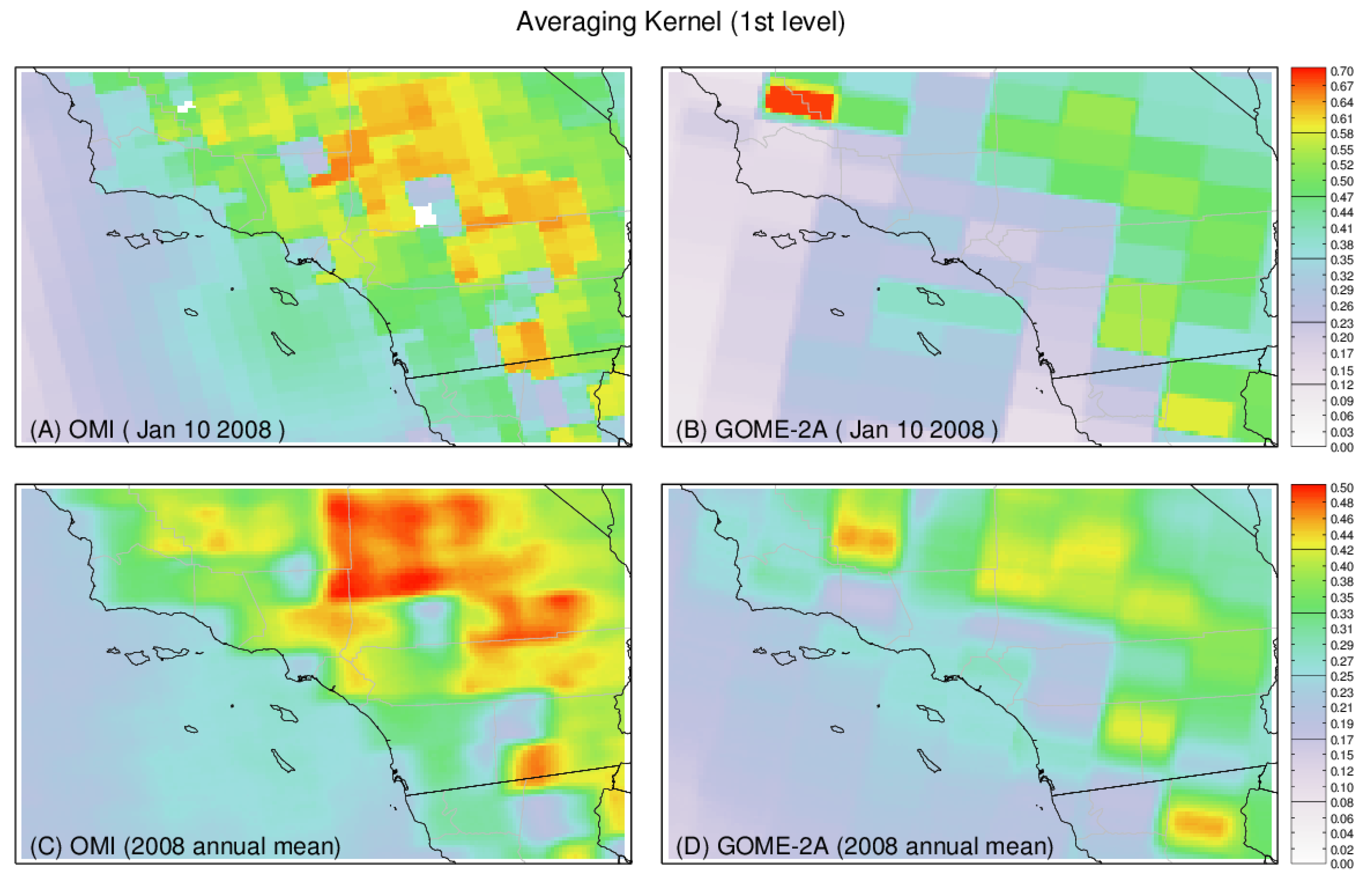
3.3. Averaging Kernel

In addition to the spatial adjustment required to match horizontal resolutions in the data, the differences in vertical properties between satellites and the model are also considered. For space-borne monitoring, the sensitivity of the instrument to tropospheric composition tends to depend on the altitude, having a vertical profile of systematic errors [46,47]. The averaging kernels (AKs), which provide an instrument’s relative sensitivity to the target tracer’s abundance, were applied to each layer’s model density, before being integrated into the column density [48]. Detailed procedures are described in Kim et al. [21].

4. Downscaling of Column Densities

Using the spatial and vertical adjustment methods from the previous section, NO₂ column densities from OMI and GOME-2 are compared here with CMAQ simulated column densities. Figure 4 shows spatial distributions of the annual mean OMI and CMAQ NO₂ column densities in 2008 over southern California. The two left-hand panels show OMI NO₂ column densities with (“DS”) and without (“xDS”) using the downscaling technique, and the two right-hand panels show CMAQ NO₂ column densities with (“AK”) and without (“xAK”) AK information. In general, both satellite and model data represent the geographical distribution of potential NO_x emission sources, including the strong emission flux signals from Los Angeles and its neighboring cities (Bakersfield, Riverside, and San Diego). However, it is also noticeable that the original OMI NO₂ column density (“xDS”) has smoother spatial distribution than the CMAQ NO₂ vertical column density or downscaled OMI NO₂ column density.

The smoothing effect due to OMI pixel size is better shown in scattered plots, and thus Figure 5 shows the comparison between OMI and CMAQ NO₂ column densities in scatter plots. Over the locations with higher NO₂ concentration, OMI tends to have lower NO₂ column densities compared with CMAQ, which is consistent with the result suggested from the smoothing effect. Using the downscaling method improves both the correlation coefficient (R = 0.96) and linear square fit slope (Slope = 1.01). Applying the AK did not make much difference.

The advantage of the downscaling technique is dramatic in the processing of GOME-2 NO₂ data, which have a larger footprint pixel size (80 × 40 km). Figure 6 shows spatial distributions of GOME-2 NO₂ column densities and modeled NO₂ column densities in the morning (~09:30 a.m.). Clearly, the GOME-2 cannot resolve fine-structure NO₂ plumes from Los Angeles or other cities. It should be noted that variant color scales are used for each plot to represent fully the spatial distributions. The maximum NO₂ column density of GOME-2 without downscaling (24 × 10¹⁵ #/cm²) is almost twice that of the same data with downscaling. However, the actual change within the whole domain is negligible considering the difference is less than 0.2% (e.g., (3.4913 − 3.4856) × 10¹⁵#/cm²/3.4913 × 10¹⁵ #/cm² × 100% = 0.16%).

Figure 7 shows scatter plot comparisons between GOME-2 NO₂ column densities and CMAQ NO₂ column densities. As previously emphasized, comparisons between GOME-2 column densities without downscaling result in extremely poor agreement when compared with the fine-scale model. When the conservative downscaling method was used, GOME-2 NO₂ column density was found to have much better agreement with modeled column densities in terms of spatial variation. It should be noted that using AK vertical adjustment results in worse comparison results. When the AK is used, the regression slope changes from 0.69 to 0.53, also with worse variations. This discrepancy may come from the coarse spatial resolution of AK distribution. Figure 8 shows examples of the first layer AK distributions on 10 January 2008 (A,B) and the annual average throughout 2008 (C,D). As the AKs are assigned per satellite pixel, they have a sharp gradient at each pixel boundary. This pattern is very clear in the layers near the surface, implying its likely association with the surface type data of the priori model. If these AKs are directly applied to the model output, they may lose their fine-scale structure due to the coarse AKs. In this case, the application of AK should be used with caution.

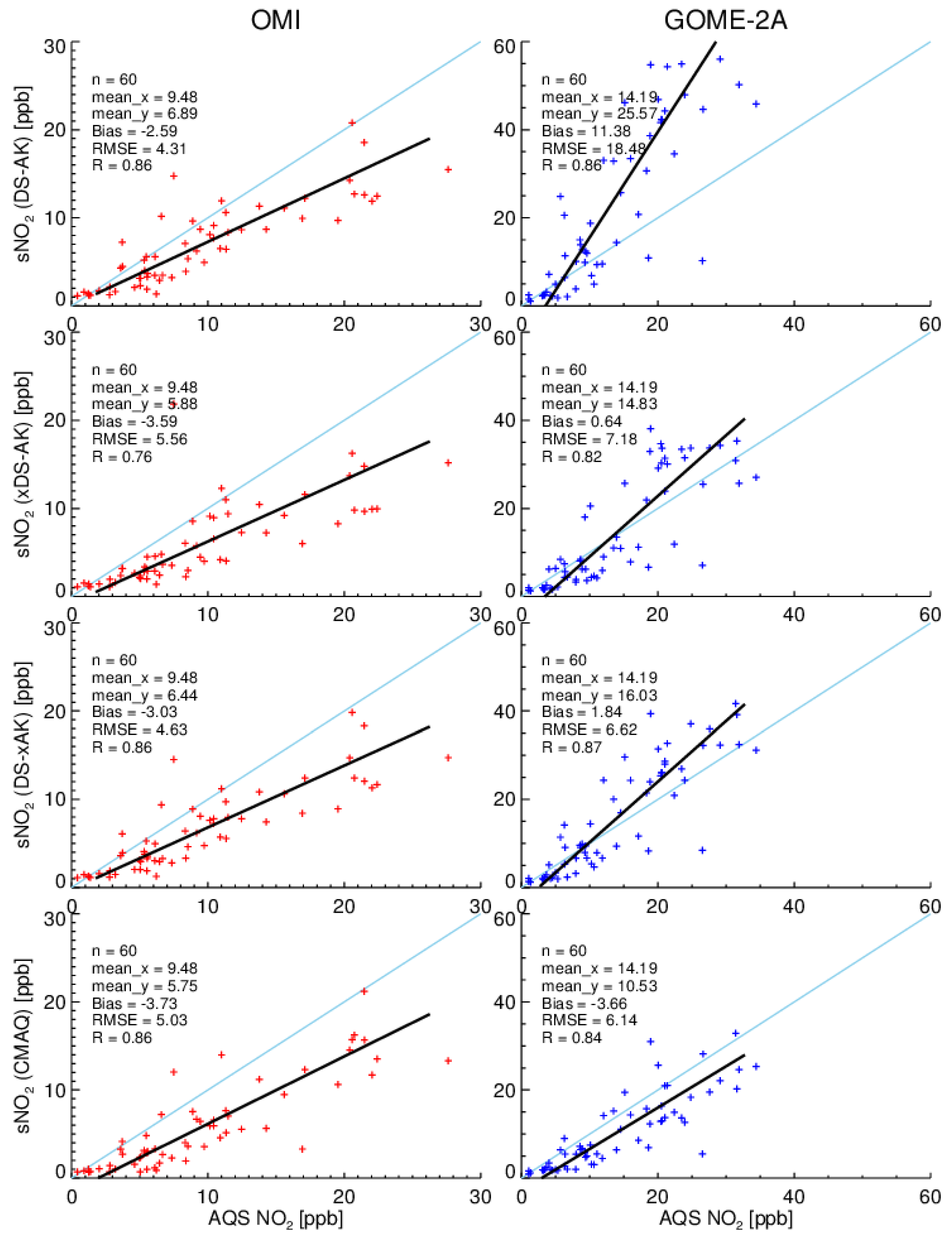
5. Reconstruction of Surface Concentration

We further estimated surface concentration using satellite observations and model simulation. Although surface concentration and column densities of NO₂ are highly associated due to their proximity to surface sources and relatively short lifetime, their correlation is not exactly linear. Following previous approaches [18,49,50,51],we converted the satellite-measured column density to surface concentration by applying the surface-to-column ratios simulated from the model. The satellite inferred surface NO₂ concentrations can be estimated as

$$\mathrm{NO}{2}_{Conc,Sat}=\mathrm{NO}{2}_{Column,Sat}·\frac{\mathrm{NO}{2}_{Conc,Mod}}{\mathrm{NO}{2}_{Column,Mod}}·\mathsf{\alpha }$$

(4)

where α is an additional adjustment due to satellite and model uncertainties. In a perfect world where satellite observations and model simulations produce true numbers, the adjustment factor α might be just one, and the surface concentration could be perfectly reconstructed using satellite observation data and the model’s surface to column ratios. However, in the real world, an additional adjustment may be required to consider uncertainties from satellite and model data, so α can be determined later to minimize the difference between reconstructed and observed surface NO₂ concentrations.

Figure 9 shows comparisons between the EPA’s AQS surface NO₂ concentrations and reconstructed NO₂ concentrations based on the model and satellite-model data. While pure model simulations produce reasonable surface concentrations, the reconstructed NO₂ concentrations using downscaled satellite and model data with AK produce the best agreement in terms of mean bias (−2.59 ppb) and correlation (R = 0.86) for OMI’s overpass time. On the other hand, GOME-2 reconstructed NO₂ concentration shows the best result, with downscaling but without AK, R = 0.87. The limitation of large AK pixels, discussed in Figure 8, may explain the deteriorated performance of GOME-2 with AK.

Further, we tried to determine α by minimizing the bias between measured and reconstructed NO₂ concentrations. For OMI reconstructed NO₂ concentration, we applied α = 1.37 (=9.48 ppb/6.89 ppb) to the case with downscaling and AK. For GOME-2 reconstructed NO₂ concentration, we applied α = 0.88 (=14.19 ppb/16.03 ppb) to the case with downscaling but without AK. In both cases, correlation coefficients remain the same, and mean biases become 0. Figure 10 and Figure 11 show the spatial distribution of reconstructed surface NO₂ concentrations overlaid with AQS surface observations. Even with the fixed α adjustment, the reconstructed NO₂ concentrations show good agreement with the observations. Better adjustment parameter α values can be found through further training of observational data sets.

One of the important findings we can draw from this study is that it is possible to maximize the capability of GOME-2. Although GOME-2 is the newest instrument, with two currently operational versions (e.g., GOME-2A and GOME-2B), its use in fine-scale research has been limited due to data resolution. In terms of spatial variability of reconstructed surface NO₂ concentration field, our results demonstrate that GOME-2 can produce a similar quality outcome to that of OMI thanks to the conservative downscaling method. This finding is encouraging because the full use of GOME-2 can add valuable information due to its morning time overpass to monitor NO_x emission signals from urban traffic.

It also should be noted that we tested the reconstruction of the surface NO₂ concentration only with a simple α value adjustment. With enhanced data assimilation skills and more training cases, the performance of surface concentration reconstruction will be improved. This was beyond the scope of the current study, and so will be pursued further in future research.

6. Conclusions

This study demonstrates an application of the conservative downscaling technique to compare atmospheric chemical composition data sets with different spatial resolutions. Due to the geometric smoothing effect, coarse resolution satellite data cannot resolve finer structures and tend to underestimate urban plumes, especially for the chemical compositions that have high spatial gradients like NO₂. Without proper adjustment, coarse resolution satellite data may be systematically underestimated in urban areas and overestimated in rural areas, which seriously misleads the evaluation of current emission inventories for air quality modeling.

The conservative downscaling technique was designed to enhance the spatial resolution of satellite measurements. Fine-scale spatial structures from the model were applied to each coarse satellite pixel to reconstruct inner structures. Downscaling was conducted for each pixel level with strict mass conservation, so it did not alter the original observed quantity at each satellite footprint pixel. With the conservative downscaling approach, NO₂ column densities from OMI and GOME-2 instruments show excellent agreement with CMAQ-simulated NO₂ column densities; R = 0.96 for OMI and R = 0.97 for GOME-2. We further constructed the surface NO₂ concentration field by combining OMI and GOME-2 satellite column densities and simulated surface-to-column ratios from the model. Compared with the EPA’s AQS surface observations, the reconstructed surface concentrations show a good agreement; R = 0.86 for both OMI and GOME-2. It is encouraging that, with the conservative downscaling, GOME-2 can produce high quality concentration fields similar to OMI, in spite of the former’s larger footprint pixels.

We conclude that the conservative downscaling approach is a useful tool to conduct a comparison between coarse-scale satellites and fine-scale models or observations in urban areas. The concept of mass conservation—treating each satellite footprint as a polygon—is essential when dealing with chemical compositions, especially when interpreted in terms of emission inventory evaluation. A reconstructed fine-scale surface concentration field that uses enhanced satellite products could also be used for future epidemiology and urbanization studies.

References

1. Chauhan, A.; Inskip, H.M.; Linaker, C.H.; Smith, S.; Schreiber, J.; Johnston, S.L.; Holgate, S.T. Personal exposure to nitrogen dioxide (NO2) and the severity of virus-induced asthma in children. Lancet 2003, 361, 1939–1944. [Google Scholar] [CrossRef]
2. Kampa, M.; Castanas, E. Human health effects of air pollution. Environ. Pollut. 2008, 151, 362–367. [Google Scholar] [CrossRef] [PubMed]
3. Jacob, D.J.; Heikes, E.G.; Fan, S.; Logan, J.A.; Mauzerall, D.L.; Bradshaw, J.D.; Singh, H.B.; Gregory, G.L.; Talbot, R.W.; Blake, D.R.; et al. Origin of ozone and NO x in the tropical troposphere: A photochemical analysis of aircraft observations over the South Atlantic basin. J. Geophys. Res. 1996, 101, 24235–24250. [Google Scholar] [CrossRef]
4. Seinfeld, J.H.; Pandis, S.N. Atmospheric Chemistry and Physics, from Air Pollution to Climate Change; John Wiley: New York, NY, USA, 1998; ISBN 0-471-17815-2. [Google Scholar]
5. Solomon, S.; Portmann, R.W.; Sanders, R.W.; Daniel, J.S.; Madsen, W.; Bartram, B.; Dutton, E.G. On the role of nitrogen dioxide in the absorption of solar radiation. J. Geophys. Res. 1999, 104, 12047–12058. [Google Scholar] [CrossRef] [Green Version]
6. Rijnders, E.; Janssen, N.A.H.; van Vliet, P.H.N.; Brunekreef, B. Personal and Outdoor Nitrogen Dioxide Concentrations in Relation to Degree of Urbanization and Traffic Density. Environ. Health Perspect. 2001, 109, 411. [Google Scholar] [CrossRef] [PubMed]
7. Ross, Z.; English, P.B.; Scalf, R.; Gunier, R.; Smorodinsky, S.; Wall, S.; Jerrett, M. Nitrogen dioxide prediction in Southern California using land use regression modeling: Potential for environmental health analyses. J. Expo. Sci. Environ. Epidemiol. 2006, 16, 106–114. [Google Scholar] [CrossRef] [PubMed]
8. Studinicka, M.; Hackl, E.; Pischinger, J.; Fangmeyer, C.; Haschke, N.; Kuhr, J.; Urbanek, R.; Neumann, M.; Frischer, T. Traffic-related NO2 and the prevalence of asthma and respiratory symptoms in seven year olds. Eur. Respir. J. 1997, 10, 2275–2278. [Google Scholar] [CrossRef]
9. Burrows, J.P.; Weber, M.; Buchwitz, M.; Rozanov, V.; Ladstätter-Weißenmayer, A.; Richter, A.; DeBeek, R.; Hoogen, R.; Bramstedt, K.; Eichmann, K.-U.; et al. The Global Ozone Monitoring Experiment (GOME): Mission Concept and First Scientific Results. J. Atmos. Sci. 1999, 56, 151–175. [Google Scholar] [CrossRef] [Green Version]
10. van der A, R.J.; Peters, D.H.M.U.; Eskes, H.; Boersma, K.F.; Van Roozendael, M.; De Smedt, I.; Kelder, H.M. Detection of the trend and seasonal variation in tropospheric NO2 over China. J. Geophys. Res. 2006, 111. [Google Scholar] [CrossRef]
11. Van der A, R.J.; Eskes, H.J.; Boersma, K.F.; van Noije, T.P.C.; Van Roozendael, M.; De Smedt, I.; Peters, D.H.M.U.; Meijer, E.W. Trends, seasonal variability and dominant NOx source derived from a ten year record of NO2 measured from space. J. Geophys. Res. 2008, 113. [Google Scholar] [CrossRef]
12. Martin, R.V.; Jacob, D.J.; Chance, K.; Kurosu, T.P.; Palmer, P.I.; Evans, M.J. Global inventory of nitrogen oxide emissions constrained by space-based observations of NO2 columns. J. Geophys. Res. 2003, 108. [Google Scholar] [CrossRef]
13. Beirle, S.; Platt, U.; Wenig, M.; Wagner, T. Highly resolved global distribution of tropospheric NO2 using GOME narrow swath mode data. Atmos. Chem. Phys. 2004, 4, 1913–1924. [Google Scholar] [CrossRef]
14. Richter, A.; Burrows, J.P.; Nüss, H.; Granier, C.; Niemeier, U. Increase in tropospheric nitrogen dioxide over China observed from space. Nature 2005, 437, 129–132. [Google Scholar] [CrossRef] [PubMed]
15. Kim, S.-W.; Heckel, A.; McKeen, S.A.; Frost, G.J.; Hsie, E.-Y.; Trainer, M.K.; Richter, A.; Burrows, J.P.; Peckham, S.E.; Grell, G.A. Satellite-observed U.S. power plant NOx emission reductions and their impact on air quality. Geophys. Res. Lett. 2006, 33. [Google Scholar] [CrossRef]
16. Konovalov, I.B.; Beekmann, M.; Richter, A.; Burrows, J.P. Inverse modelling of the spatial distribution of NOx emissions on a continental scale using satellite data. Atmos. Chem. Phys. 2006, 6, 1747–1770. [Google Scholar] [CrossRef]
17. Boersma, K.F.; Eskes, H.J.; Veefkind, J.P.; Brinksma, E.J.; van der A, R.J.; Sneep, M.; van den Oord, G.H.J.; Levelt, P.F.; Stammes, P.; Gleason, J.F.; Bucsela, E.J. Near-real time retrieval of tropospheric NO2 from OMI. Atmos. Chem. Phys. 2007, 7, 2103–2118. [Google Scholar] [CrossRef]
18. Lamsal, L.N.; Martin, R.V.; van Donkelaar, A.; Steinbacher, M.; Celarier, E.A.; Bucsela, E.; Dunlea, E.J.; Pinto, J.P. Ground-level nitrogen dioxide concentrations inferred from the satellite-borne Ozone Monitoring Instrument. J. Geophys. Res. 2008, 113. [Google Scholar] [CrossRef] [Green Version]
19. Napelenok, S.L.; Pinder, R.W.; Gilliland, A.B.; Martin, R.V. A method for evaluating spatially-resolved NOx emissions using Kalman filter inversion, direct sensitivities, and space-based NO2 observations. Atmos. Chem. Phys. 2008, 8, 5603–5614. [Google Scholar] [CrossRef]
20. Kim, S.-W.; Heckel, A.; Frost, G.J.; Richter, A.; Gleason, J.; Burrows, J.P.; McKeen, S.; Hsie, E.-Y.; Granier, C.; Trainer, M. NO2 columns in the western United States observed from space and simulated by a regional chemistry model and their implications for NOx emissions. J. Geophys. Res. 2009, 114. [Google Scholar] [CrossRef]
21. Kim, H.C.; Lee, P.; Judd, L.; Pan, L.; Lefer, B. OMI NO2 column densities over North American urban cities: The effect of satellite footprint resolution. Geosci. Model Dev. 2016, 9, 1111–1123. [Google Scholar] [CrossRef]
22. Russell, A.R.; Perring, A.E.; Valin, L.C.; Bucsela, E.J.; Browne, E.C.; Wooldridge, P.J.; Cohen, R.C. A high spatial resolution retrieval of NO2 column densities from OMI: Method and evaluation. Atmos. Chem. Phys. 2011, 11, 8543–8554. [Google Scholar] [CrossRef]
23. Boersma, K.F.; Jacob, D.J.; Bucsela, E.J.; Perring, A.E.; Dirksen, R.; van der A, R.J.; Yantosca, R.M.; Park, R.J.; Wenig, M.O.; Bertram, T.H. Validation of OMI tropospheric NO2 observations during INTEX-B and application to constrain NOxNOx emissions over the eastern United States and Mexico. Atmos. Environ. 2008, 42, 4480–4497. [Google Scholar] [CrossRef] [Green Version]
24. Palmer, P.I.; Jacob, D.J.; Chance, K.; Martin, R.V.; Spurr, R.J.D.; Kurosu, T.P.; Bey, I.; Yantosca, R.; Fiore, A.; Li, Q. Air mass factor formulation for spectroscopic measurements from satellites: Application to formaldehyde retrievals from the Global Ozone Monitoring Experiment. J. Geophys. Res. 2001, 106. [Google Scholar] [CrossRef]
25. Schaub, D.; Brunner, D.; Boersma, K.F.; Keller, J.; Folini, D.; Buchmann, B.; Berresheim, H.; Staehelin, J. SCIAMACHY tropospheric NO2 over Switzerland: Estimates of NOx lifetimes and impact of the complex Alpine topography on the retrieval. Atmos. Chem. Phys. 2007, 7, 5971–5987. [Google Scholar] [CrossRef]
26. Skamarock, W.C.; Klemp, J.B. A time-split nonhydrostatic atmospheric model for weather research and forecasting applications. J. Comput. Phys. 2008, 227, 3465–3485. [Google Scholar] [CrossRef]
27. Janjic, Z.I.; Gerrity, J.P.; Nickovic, S. An Alternative Approach to Nonhydrostatic Modeling. Mon. Weather Rev. 2001, 129, 1164–1178. [Google Scholar] [CrossRef]
28. Hong, S.-Y.; Noh, Y.; Dudhia, J. A new vertical diffusion package with an explicit treatment of entrainment processes. Mon. Weather Rev. 2006, 134, 2318–2341. [Google Scholar] [CrossRef]
29. Hong, S.-Y.; Dudhia, J.; Chen, S.-H. A Revised Approach to Ice Microphysical Processes for the Bulk Parameterization of Clouds and Precipitation. Mon. Weather Rev. 2004, 132, 103–120. [Google Scholar] [CrossRef] [Green Version]
30. Mlawer, E.J.; Taubman, S.J.; Brown, P.D.; Iacono, M.J.; Clough, S.A. Radiative transfer for inhomogeneous atmospheres: RRTM, a validated correlated-k model for the longwave. J. Geophys. Res. Atmos. 1997, 102, 16663–16682. [Google Scholar] [CrossRef] [Green Version]
31. Dudhia, J. Numerical Study of Convection Observed during the Winter Monsoon Experiment Using a Mesoscale Two-Dimensional Model. J. Atmos. Sci. 1989, 46, 3077–3107. [Google Scholar] [CrossRef] [Green Version]
32. Kain, J.S. The Kain–Fritsch Convective Parameterization: An Update. J. Appl. Meteorol. 2004, 43, 170–181. [Google Scholar] [CrossRef]
33. South Coast Air Quality Management District (SCAQMD). Air Quality Management Plan 2012; South Coast Air Quality Management District: Diamond Bar, CA, USA, 2013. [Google Scholar]
34. Carter, W.P.L. Documentation of the SAPRC-99 Chemical Mechanism for VOC Reactivity Assessment. Assessment 1999, 1, 329. [Google Scholar]
35. Pleim, J.E. A Combined Local and Nonlocal Closure Model for the Atmospheric Boundary Layer. Part II: Application and Evaluation in a Mesoscale Meteorological Model. J. Appl. Meteorol. Climatol. 2007, 46, 1396–1409. [Google Scholar] [CrossRef]
36. Boersma, K.F.; Eskes, H.J.; Brinksma, E.J. Error analysis for tropospheric NO2 retrieval from space. J. Geophys. Res. 2004, 109. [Google Scholar] [CrossRef]
37. United States Environmental Protection Agency (EPA). Technical Assistance Document for the Chemiluminescence Measurement of Nitrogen Dioxide; United States Environmental Protection Agency: Research Triangle Park, NC, USA, 1975.
38. Steinbacher, M.; Zellweger, C.; Schwarzenbach, B.; Bugmann, S.; Buchmann, B.; Ordóñez, C.; Prevot, A.S.H.; Hueglin, C. Nitrogen oxide measurements at rural sites in Switzerland: Bias of conventional measurement techniques. J. Geophys. Res. 2007, 112. [Google Scholar] [CrossRef] [Green Version]
39. Bechle, M.J.; Millet, D.B.; Marshall, J.D. Remote sensing of exposure to NO2: Satellite versus ground-based measurement in a large urban area. Atmos. Environ. 2013, 69, 345–353. [Google Scholar] [CrossRef]
40. Houyoux, M.R.; Vukovich, J.M.; Coats, C.J.; Wheeler, N.J.M.; Kasibhatla, P.S. Emission inventory development and processing for the Seasonal Model for Regional Air Quality (SMRAQ) project. J. Geophys. Res. 2000, 105, 9079–9090. [Google Scholar] [CrossRef] [Green Version]
41. Fruchter, A.S.; Hook, R.N. Drizzle: A Method for the Linear Reconstruction of Undersampled Images. Publ. Astron. Soc. Pac. 2002, 114, 144–152. [Google Scholar] [CrossRef] [Green Version]
42. Smith, J.D.T.; Armus, L.; Dale, D.A.; Roussel, H.; Sheth, K.; Buckalew, B.A.; Jarrett, T.H.; Helou, G.; Kennicutt, R.C., Jr. Spectral Mapping Reconstruction of Extended Sources. Publ. Astron. Soc. Pac. 2007, 119, 1133–1144. [Google Scholar] [CrossRef] [Green Version]
43. Sutherland, I.E.; Hodgman, G.W. Reentrant polygon clipping. Commun. ACM 1974, 17, 32–42. [Google Scholar] [CrossRef]
44. Kim, H.; Ngan, F.; Lee, P.; Tong, D. Development of IDL-Based Geospatial Data Processing Framework for Meteorology and Air Quality Modeling; Air Quality Research Program Agency: Austin, TX, USA, 2013. [Google Scholar]
45. Goldberg, D.L.; Lamsal, L.N.; Loughner, C.P.; Swartz, W.H.; Lu, Z.; Streets, D.G. A high-resolution and observationally constrained OMI NO2 satellite retrieval. Atmos. Chem. Phys. 2017, 17, 11403–11421. [Google Scholar] [CrossRef]
46. Eskes, H.J.; Boersma, K.F. Averaging kernels for DOAS total-column satellite retrievals. Atmos. Chem. Phys. 2003, 3, 1285–1291. [Google Scholar] [CrossRef] [Green Version]
47. Bucsela, E.J.; Perring, A.E.; Cohen, R.C.; Boersma, K.F.; Celarier, E.A.; Gleason, J.F.; Wenig, M.O.; Bertram, T.H.; Wooldridge, P.J.; Dirksen, R.; et al. Comparison of tropospheric NO2 from in situ aircraft measurements with near-real-time and standard product data from OMI. J. Geophys. Res. 2008, 113. [Google Scholar] [CrossRef]
48. Herron-Thorpe, F.L.; Lamb, B.K.; Mount, G.H.; Vaughan, J.K. Evaluation of a regional air quality forecast model for tropospheric NO2 columns using the OMI/Aura satellite tropospheric NO2 product. Atmos. Chem. Phys. 2010, 10, 8839–8854. [Google Scholar] [CrossRef]
49. Gu, J.; Chen, L.; Yu, C.; Li, S.; Tao, J.; Fan, M.; Xiong, X.; Wang, Z.; Shang, H.; Su, L. Ground-Level NO2 Concentrations over China Inferred from the Satellite OMI and CMAQ Model Simulations. Remote Sens. 2017, 9, 519. [Google Scholar] [CrossRef]
50. Kharol, S.K.; Martin, R.V.; Philip, S.; Boys, B.; Lamsal, L.N.; Jerrett, M.; Brauer, M.; Crouse, D.L.; McLinden, C.; Burnett, R.T. Assessment of the magnitude and recent trends in satellite-derived ground-level nitrogen dioxide over North America. Atmos. Environ. 2015, 118, 236–245. [Google Scholar] [CrossRef]
51. McLinden, C.A.; Fioletov, V.; Boersma, K.F.; Kharol, S.K.; Krotkov, N.; Lamsal, L.; Makar, P.A.; Martin, R.V.; Veefkind, J.P.; Yang, K. Improved satellite retrievals of NO2 and SO2 over the Canadian oil sands and comparisons with surface measurements. Atmos. Chem. Phys. 2014, 14, 3637–3656. [Google Scholar] [CrossRef]
Figure 1. Geographical coverage of study domain over southern California. Circles represent annual mean surface NO2 concentrations from the EPA’s AQS surface monitoring sites.
Remotesensing 10 01001 g001
Figure 2. Example of the conservative regridding method. OMI NO2 column densities are regridded onto a 4-km model domain using fractional weighting. (A) Original OMI NO2 column density; (B) zoomed in feature (blue box in (A)); and (C) regridded OMI NO2 column densities are shown.
Remotesensing 10 01001 g002
Figure 3. Example of the conservative downscaling of GOME-2 NO2 column densities. (A) Original GOME-2 NO2 column densities; (B) CMAQ NO2 column densities; (C) spatial weighting kernel; and (D) downscaled GOME-2 NO2 column densities are shown.
Remotesensing 10 01001 g003
Figure 4. Spatial distribution of OMI and CMAQ NO2 column densities. “DS” and “xDS” denote OMI NO2 column densities with and without the downscaling method, respectively, whereas “AK” and “xAK” denote CMAQ NO2 column densities with and without the averaging kernel, respectively.
Remotesensing 10 01001 g004
Figure 5. Scatter plot comparison of OMI and CMAQ NO2 column densities. “DS” and “xDS” denote OMI NO2 column densities with and without the downscaling method, respectively, whereas “AK” and “xAK” denote CMAQ NO2 column densities with and without the averaging kernel, respectively.
Remotesensing 10 01001 g005
Figure 6. Spatial distribution of GOME-2 and CMAQ NO2 column densities. “DS” and “xDS” denote GOME-2 NO2 column densities with and without the downscaling method, respectively, whereas “AK” and “xAK” denote CMAQ NO2 column densities with and without the averaging kernel, respectively.
Remotesensing 10 01001 g006
Figure 7. Scatter plot comparison of GOME-2 and CMAQ NO2 column densities. “DS” and “xDS” denote GOME-2 NO2 column densities with and without the downscaling method, respectively, whereas “AK” and “xAK” denote CMAQ NO2 column densities with and without the averaging kernel, respectively.
Remotesensing 10 01001 g007
Figure 8. Spatial distribution of OMI and GOME-2 averaging kernel at the first layer on 10 January 2008 (A,B), and averaged in 2008 (C,D).
Remotesensing 10 01001 g008
Figure 9. Comparisons of reconstructed NO2 concentrations based on satellite and model data, and the EPA’s AQS surface NO2 concentrations. “DS” and “xDS” denote with and without downscaling technique, and “AK” and “xAK” denote with and without averaging kernel.
Remotesensing 10 01001 g009
Figure 10. Reconstructed surface NO2 concentrations using OMI column densities and CMAQ column-to-surface ratios at 13:30 local time in 2008.
Remotesensing 10 01001 g010
Figure 11. Reconstructed surface NO2 concentrations using GOME-2 column densities and CMAQ column-to-surface ratios at 09:30 local time in 2008.
Remotesensing 10 01001 g011