Spatio-Temporal Super-Resolution Land Cover Mapping Based on Fuzzy C-Means Clustering


1
National Engineering Research Center of Geographic Information System, China University of Geosciences, Wuhan 430074, China
2
Institute of Geodesy and Geophysics, Chinese Academy of Sciences, Wuhan 430077, China
3
School of Geography and Planning, Sun Yat-sen University, Guangzhou 510275, China
*
Author to whom correspondence should be addressed.
Remote Sens. 2018, 10(8), 1212; https://doi.org/10.3390/rs10081212
Submission received: 20 July 2018
/
Revised: 29 July 2018
/
Accepted: 31 July 2018
/
Published: 2 August 2018
(This article belongs to the Special Issue Remote Sensing Image Downscaling)
Abstract
:Super-resolution land cover mapping (SRM) is a method that aims to generate land cover maps with fine spatial resolutions from the original coarse spatial resolution remotely sensed image. The accuracy of the resultant land cover map produced by existing SRM methods is often limited by the errors of fraction images and the uncertainty of spatial pattern models. To address these limitations in this study, we proposed a fuzzy c-means clustering (FCM)-based spatio-temporal SRM (FCM_STSRM) model that combines the spectral, spatial, and temporal information into a single objective function. The spectral term is constructed with the FCM criterion, the spatial term is constructed with the maximal spatial dependence principle, and the temporal term is characterized by the land cover transition probabilities in the bitemporal land cover maps. The performance of the proposed FCM_STSRM method is assessed using data simulated from the National Land Cover Database dataset and real Landsat images. Results of the two experiments show that the proposed FCM_STSRM method can decrease the influence of fraction errors by directly using the original images as the input and the spatial pattern uncertainty by inheriting land cover information from the existing fine resolution land cover map. Compared with the hard classification and FCM_SRM method applied to mono-temporal images, the proposed FCM_STSRM method produced fine resolution land cover maps with high accuracy, thus showing the efficiency and potential of the novel approach for producing fine spatial resolution maps from coarse resolution remotely sensed images.

1. Introduction
Land cover and its change are one of the most prominent landscape signs to record the characteristic and dynamic processes of the Earth’s surface [1,2]. With the development of remote sensing technology in recent years, land cover information can be acquired from remote sensing images with different spatial and temporal resolutions [3]. In general, a land cover map is produced by the hard classification method, which assigns each pixel in the remotely sensed image to a certain land cover class. However, the remotely sensed image pixels are often mixed with several different land cover classes, particularly the pixels located in the land cover patch boundaries in coarse spatial resolution images. Pixel based hard classification methods always ignore the mixed pixel phenomena and only use the statistical characteristics of the pixel spectra to classify a mixed pixel as a specific land cover type, such that the resultant land cover map cannot accurately represent the land cover information. A well-known method to address the limitation of hard classification is the use of soft classification, which is also called spectral unmixing. Soft classification can extract the area percentage of each land cover class in mixed pixels and obtain more accurate land cover information than hard classification. However, soft classification does not give the spatial distribution of land cover classes at the subpixel level and the spatial resolution of classification result does not really improved.
Super-resolution mapping (SRM) or subpixel mapping, which aims to generate land cover map with fine spatial resolutions from original coarse spatial resolution remotely sensed images, was subsequently proposed to address the previously mentioned limitations of hard classification and soft classification [4,5,6]. In SRM, one coarse spatial resolution pixel is initially divided into subpixels according to the zoom factor. Then, the subpixel number, which is calculated for each land cover class based on the fraction images derived from the soft classification, is used as the input. Finally, the spatial locations of these subpixels are determined according to a certain spatial prior model to produce the fine spatial resolution land cover map [7,8,9]. Various SRM algorithms, including pixel-swapping algorithms [10,11], fuzzy c-means clustering (FCM)-based algorithms [12,13], Markov random field based algorithms [14,15], and learning-based algorithms [16], have been proposed in the past two decades. SRM has also been successfully used in many relative fields, such as forest mapping [17,18,19], waterline mapping [20,21,22], and urban tree mapping [12].
In theory, SRM is an inversion problem because it needs to recover missing subpixel information from the observed coarse spatial resolution images. Various spatial models, such as the maximal spatial dependence model and the linear spatial model, have been proposed to provide land cover distribution information at the subpixel scale for SRM. However, applying SRM with a single coarse resolution image is always limited because no subpixel information is used, and using the spatial prior model only is insufficient to produce with high accuracy the resultant fine resolution land cover map [7]. Incorporating the additional site-specific dataset, such as panchromatic band images [23,24], LIDAR data [25], and vector boundaries [26,27], into SRM can overcome this problem to a large extent. These additional datasets can provide useful spatial land cover information for SRM and reduce the uncertainty of the resultant land cover map. However, the effectiveness of this kind of method is limited by the availability and quality of additional datasets, for example, the acquired time of the fraction images and the additional datasets should be the same or similar.
Notably, abundant archived fine spatial resolution land cover maps or remotely sensed images exist globally. These archived fine spatial resolution datasets can provide a valuable prior land cover pattern for SRM, leading to the spatio-temporal SRM (STSRM) [28]. STSRM aims to generate a high-resolution land cover map from a coarse resolution remotely sensed image by incorporating a former high-resolution land cover map. STSRM is not only considered an extension of traditional SRM approaches that are applied with a single coarse resolution image, but it can also be considered a spatio-temporal land cover fusion method because of the combined advantages of short cycle times of coarse spatial resolution images and rich spatial feature information of fine spatial resolution images, and then generate a series of fine spatial and temporal resolution land cover maps. Many different STSRM methods, such as the spatio-temporal Markov random field based SRM model [15], spatio-temporal pixel-swapping model [29], and Hopfield neural network based fast STSRM model [30] have been proposed in recent years.
In general, existing STSRM models often uses a previous fine spatial resolution land cover map and current coarse spatial resolution fraction images as input to estimate the current fine spatial resolution land cover map. The previous fine spatial resolution land cover map can be a documented dataset or produced by classifying a fine resolution remote sensing image. Coarse spatial resolution fraction images are always estimated from remotely sensed images by soft classification. Existing models often assume that the input datasets are error free; however, this assumption is problematic because errors are unavoidable for the input datasets, particularly for the coarse resolution fraction images generated by soft classification. In order to overcome this shortcoming, a sub-pixel land cover fraction change detection method is often first applied in practice, and STSRM is then only applied in those coarse resolution pixels with land cover fraction changes [31]. However, this method is still limited by the accuracy of change detection. Given that the errors of fraction images are caused by soft classification, if the spectral information can be considered directly in the STSRM model, then the STSRM result is expected to be improved.
The FCM algorithm, which adopts fuzziness membership values to analyze the spectral information of remotely sensed images, has been widely used as a soft classification algorithm to provide land cover fraction images [32,33]. Then, in SRM, as FCM can generate different fraction images by using different fuzziness parameters, it is usually utilized as the preprocessing step to generate the input fraction images [9]. Although the FCM can provide flexible choices of fraction images, it still would carry uncertainty to the SRM result. To overcome this shortcoming, FCM was further applied to image-based SRM methods. Li et al. proposed an FCM-based SRM (FCM_SRM) model that incorporates the pixel-unmixing criterion of sFCM into its objective function [9]. Zhang et al. extended the FCM_SRM model into an unsupervised model [34]. Compared with SRM methods that use the fraction images generated by soft classification as input, these image-based SRM methods use the FCM criterion applied to the original coarse spatial resolution images and can eliminate the influence of fraction errors on the resultant fine resolution land cover map to some extent.
Given that image-based SRM models that use the FCM criterion can overcome the propagation of fraction error on the SRM result, applying this kind of method in existing STSRM models is expected to overcome the limitation of handling fraction uncertainty. Therefore, in this study, we introduced the FCM algorithm into STSRM and proposed a FCM-based STSRM (FCM_STSRM) method, which considers the fuzziness of the pixels under the STSRM framework. The proposed FCM_STSRM method fully incorporates the spectral, spatial, and temporal information included in the input dataset, that is, the FCM criterion for spectral unmixing, the spatial pattern of land cover, and the temporal pattern of land cover change.
2. Methods
2.1. FCM_STSRM
The objective of FCM_STSRM is to estimate a fine spatial resolution land cover map from the observed coarse spatial resolution remotely sensed image with the aid of the existing former fine spatial resolution land cover map. Suppose that the coarse spatial resolution remotely sensed image is with bands, each contains pixels with the spatial resolution . The former fine spatial resolution land cover map is with the spatial resolution . The zoom factor is , indicating that each coarse resolution pixel in includes fine resolution pixels in . Therefore, FCM_STSRM aims to predict a fine spatial resolution land cover map at the time of coarse spatial remotely sensed image observation, including pixels with the spatial resolution .
According to the maximum a posteriori rule in the Bayesian framework, the resultant land cover map is calculated on the basis of the given map and coarse spatial resolution remotely sensed image . Therefore, the optimal result can be estimated by solving the maximization problem, as follows:
where is a normalizing constant; is the posterior probability of ; and is the corresponding posterior energy function of , given and .
On the basis of the Markov random field approach, the search for the optimal is equivalent to minimization of the posterior energy function, which can be specified to model the spatial and temporal dependencies of pixels on its spatial and temporal neighborhoods [35], as follows:
where is the spectral energy function that provides the constraints of observed coarse spatial resolution images in the output fine spatial resolution land cover map ; is the spatial energy function that is used to ensure that the output fine spatial resolution land cover map satisfies a predefined spatial pattern; is the temporal energy function that is used to measure the temporal dependence between and ; and and are the weighting coefficients that control the weights of the spectral, spatial, and temporal terms.
2.2. Spectral Term
The spectral term is used to link the observed coarse spatial resolution image with the resultant fine spatial resolution land cover map . Here, the FCM criterion is adopted to construct the spectral term.
In general, the FCM is an unsupervised clustering algorithm that assigns pixels to each category by using fuzzy memberships. Suppose the sample set , is the D-dimensional feature vector. The FCM aims to cluster these samples into C classes by using an iterative optimization that minimizes the objective function defined as follows:
with the following constraints:
where is the fuzzy membership of pixel in the i-th cluster; is the number of classes; is a norm metric; m is a constant called fuzziness parameter; is the i-th cluster center; and is a weighting exponent on each fuzzy membership that controls the fuzziness of the analysis.
The FCM criterion has been widely used for spectral unmixing. In general, the fuzzy membership, that is, , can be applied to represent the fraction value of the class in the coarse resolution pixel . If the endmember of the land cover class is known, then the unsupervised FCM algorithm can be adopted to be a supervised model with the following objective function:
where is the coarse resolution pixel ; is the zoom factor; and is the endmember spectral vector of class .
For SRM, the FCM criterion for the spectral term is further modified, in which is used instead of . , which is the number of fine resolution pixels labeled as in coarse resolution pixel , is utilized in calculating as follows:
Therefore, the spectral energy is ultimately calculated as follows:
2.3. Spatial Term
The spatial term is used to describe the spatial pattern of land cover distribution. Here, the maximal spatial dependence model, which aims to maximize the spatial neighborhood correlation among the fine spatial resolution pixels, is used. The spatial term is expressed as follows:
where is the fine resolution pixel in the coarse resolution pixel ; is the neighboring fine resolution pixel of ; is the spatial neighborhoods. is used to express the spatial dependence. When fine resolution pixel and are assigned to the same land cover class, the value of equals to −1; otherwise, it equals to 0.
The neighboring fine resolution pixels at different distances has different influences on the center fine resolution pixel . In this paper, is utilized to express the influence weight [7]. A Gaussian function of the distance between and is used to calculate the influence weight as follows:
where is a nonlinear parameter; is the distance between the two fine resolution pixels and . is the normalization constant to ensure .
2.4. Temporal Term
The temporal term is used to link the former fine spatial resolution land cover map with the resultant fine spatial resolution land cover map . In this paper, the land cover transfer matrix was employed to represent their relationship. The transfer matrix is calculated for each coarse resolution pixel one by one. Suppose there are C land cover classes, then the transfer matrix is a -sized matrix. The elements of the transfer matrix represent the transition probability that land cover class at the former time transformed into the land cover class at the latter time of coarse resolution remote sensing image acquirement, expressed as follows:
where is the transition probability; is the class label of the former coarse resolution pixel degraded from the fine resolution map; and is the class label of the pixel in the latter coarse resolution fraction images.
The transfer matrix is calculated based on the land cover change rule. In general, land cover change can be classified into three groups [23]:
(1) The first category is “equal class ”, which indicates that the fine resolution pixels of this land cover class do not change. Under this change rule, the transition probability of the “equal class ” can be calculated as follows:
(2) The second category is “increase class ”, which indicates that the fine resolution pixels of this land cover class in the latter map is more than those in the former map. In this situation, fine resolution pixels of this land cover class in the former map are all transformed into this land cover class in latter map, and fine resolution pixels of other land cover classes are transformed into this land cover class, but the fine resolution pixels of this land cover class are not transformed into other land cover class. Based on this change rule, the transition probability of the “increase class ” can be calculated as follows:
(3) The third category is “decrease class ”, which indicates that the fine resolution pixels of this land cover class in the latter map is less than those in the former map. In this situation, fine resolution pixels of this land cover class in the former map are only partly transformed into this land cover class in the latter map, and fine resolution pixels of this land cover class are transformed into other land cover classes, but other land cover classes are not transformed into this land cover class. Therefore, the transition probability of the “decrease class ” can be calculated as follows:
where and are the areas of class in the latter and former maps. and are the areas of class in the latter and former maps, respectively.
A simple example is used here to illustrate the change strategy in Figure 1. In this example, the zoom factor is 10; hence, every coarse resolution pixel contains fine resolution pixels. The four land cover classes are A, B, C, and D, in which the land cover proportions are [0.36, 0.12, 0.30, 0.22] and [0.18, 0.12, 0.38, 0.32] in the former and latter maps, respectively. Accordingly, 36 fine resolution pixels are labeled as class A, 12 fine resolution pixels are labeled as class B, 30 fine resolution pixels are labeled as class C, and 22 fine resolution pixels are labeled as class D (Figure 1a). With the passage of time, land cover changes. The fraction changes of each class are computed by using the former and latter fraction images (Figure 1b). The potential fine resolution pixel locations of class A, which is a decrease class, are determined to be the former fine resolution pixels of class A (Figure 1c); some will need to relabeled to classes C and D according to the transfer matrix. The fine resolution pixel locations of class B, which is an equal class, are determined to be the former fine resolution pixels of class B (Figure 1d). The fine resolution pixel locations of classes C and D, which are increase classes, are determined to be the former fine resolution pixels of classes C and D plus potentially some of the locations labeled as class A in the former data (Figure 1e,f).
The previously presented example data were used to illustrate the entire procedure for generating the transfer matrix further (Figure 2). First, for the “equal class B”, the element [2, 2] is set to 1, and other elements in the entire second row and column are set to 0. Second, for the “increase class C and D”, the elements [3, 3] and [4, 4] are set to 1. Elements in the third and fourth columns are set to 0, excluding [3, 3] and [4, 4]. Third, for the “decrease class A”, the element [1, 1] is set to 0.18/0.36 = 1/2. Other elements are calculated with Formula (14), for example, element [1, 3] is set to . Finally, the transfer matrix of this coarse pixel is generated.
On the basis of the transfer matrix, the objective function of the temporal term can be calculated as follows:
where is the transition probability and is the fine spatial resolution pixel in coarse pixel .
2.5. Model Implementation and Accuracy Validation
The resultant fine resolution land cover map is produced by optimizing the objective function in Formula (2). Minimizing the global energy for the entire image is not analytically tractable because of the large configuration space of the problem. Iterative Conditional Model (ICM), which has the advantage of fast convergence speed, was utilized to achieve the global energy minima. The flowchart of the proposed STFCM_SRM is shown in Figure 3, and the main steps are summarized as follows:
- (1)
- The endmember spectra are extracted from the coarse resolution remotely sensed image.
- (2)
- The fraction images are produced by unmixing the coarse resolution remotely sensed image by using the extracted endmembers.
- (3)
- The SR map is initialized according to the number of subpixels for all land cover classes in each coarse resolution pixel on the basis of the fraction image.
- (4)
- The transfer matrix is calculated for every coarse resolution pixel one after another by using the fraction images and the former fine resolution land cover map.
- (5)
- Subpixel labels in the initial fine spatial resolution land cover map are updated iteratively. The land cover type for each subpixel that contributes to the minimal posterior energy is accepted as the label of this subpixel. The iteration is terminated when the previously fixed number of iteration is achieved or the algorithm converges.
Accuracy validation was achieved by comparing the resultant land cover map and the reference fine resolution land cover map pixel by pixel. The result accuracy of the proposed method was evaluated using a series of indices, including kappa coefficient, overall accuracy (OA), PULC, PCLC, KULC, and KCLC. Here, PULC is the correctly labeled percentage of the unchanged land cover pixels; PCLC is the correctly labeled percentage of the changed land cover pixels; KULC is the kappa coefficient for the unchanged land covers; and KCLC is the kappa coefficient for the changed land covers.
3. Results
3.1. Experiment 1
3.1.1. Data Preparation
In this experiment, synthetic images were used to assess the performance of the proposed FCM_STSRM method. Multispectral remote sensing images were simulated from the National Land Cover Database (NLCD), which has been applied consistently across the United States at a spatial resolution of 30 m [36]. The study area covering 2.4 × 2.4 km2 with pixels is located in Charlotte. The former finer resolution map was obtained from NLCD 2001 (Figure 4a), and the reference map used for model validation was obtained from NLCD 2006 (Figure 4b). The level I classification of NLCD with eight land cover classes including water, developed, barren, forest, shrubland, herbaceous, planted, and wetlands, was used. The changed pixels account for 8.09% of all pixels in the study area.
The fine resolution land cover map in 2006 was degraded with z = 4, z = 8, and z = 16 to simulate coarse resolution multispectral images with different spatial resolutions. The number of bands was set to seven to accommodate a dimensionality constraint in spectral unmixing. The eight endmembers were set to , , , , , , , and , where T is the transposition operator. The spectral response of each class was normally distributed in each waveband, and the covariance matrices for all of the classes were set to , where = 0.01 is a constant and is a identity matrix [11]. Three degraded images produced by different zoom factors are shown in Figure 5.
3.1.2. Model Implementation
In the proposed FCM_STSRM, the fine resolution map obtained from NLCD 2001 and the simulated coarse resolution image in 2006 were used to generate the resultant fine resolution map in 2006, and the reference map obtained from NLCD 2006 was used for model validation. The neighborhood window was set to seven, which indicates that the object fine resolution pixel has 48 neighboring fine resolution pixels. The endmembers were directly set as the simulated values.
Two additional approaches, hard classification (HC) and fuzzy c-means clustering based SRM (FCM_SRM), were used for comparison. In the HC method, the fuzzy membership of each pixel belonging to each land cover class is calculated. Then, the pixel class label is assigned according to the maximum membership. The FCM_SRM method is a SRM algorithm that is applied to a mono-temporal image without considering the temporal information. Indeed, when the temporal coefficient of FCM_STSRM is set to 0, the STFCM_SRM method degrades to FCM_SRM. All of the algorithms were tested on an Intel® Core™ i5-3470 CPU @ 3.20 GHz with 4 GB RAM with MATLAB R2016b version (The MathWorks, Inc., Natick, MA, USA).
3.1.3. Results
HC, FCM_SRM, and FCM_STSRM at different zoom factors were applied for comparison to validate the performance of the proposed method. In this experiment, the spatial and temporal coefficients are set to have the optimal values. The resultant land cover maps generated by the three different methods at z = 4, z = 8, and z = 16 are shown in Figure 6.
A visual comparison of the results shown in Figure 6 indicates that the proposed FCM_STSRM method prevailed over the two other methods at all zoom factors. With the increase in zoom factors, the detailed land cover spatial pattern is more difficult to reproduce. Compared with the reference map, HC generated land cover maps with low continuity and jagged boundaries, particularly when the zoom factor value is high (Figure 6c) because, in the HC method, land cover information is considered only at the pixel level and detailed spatial information is easily lost. Compared with the HC method, the FCM_SRM method uses maximal spatial dependence to consider the spatial neighborhood relationship. The FCM_SRM method can provide spatial information at the subpixel scale and generate a better resultant land cover map to some extent. However, the linear features cannot be easily mapped by the FCM_SRM method. Moreover, when the zoom factor increases, the resultant land cover map becomes locally smooth because the maximal spatial dependence model cannot represent the land cover pattern accurately.
By contrast, the resultant land cover map generated by FCM_STSRM can retain the fine spatial pattern and is similar to the reference map. The FCM_STSRM method considers the uncertainty in the process of spectral unmixing by using the FCM criterion under the framework of STSRM, which adds the temporal term to the FCM_STSRM algorithm. Incorporating the land cover information into the former fine resolution map can provide valuable spatial pattern for the latter land cover map. In the areas without land cover change, the resultant land cover map can inherit the land cover information from the former NLCD 2001 map directly. In this experiment, the change percentage from NLCD 2001 to NLCD 2006 is only 8.09%. Therefore, the FCM_STSRM method can generate the resultant land cover map with a high accuracy, even at a high zoom factor (such as z = 16, Figure 6i).
The accuracy assessment of the three methods is shown in Table 1. The result accuracies decreased with the increased zoom factor for all three methods because the uncertainty increased when the zoom factor increased. Compared with the result generated from HC, FCM_SRM has higher overall accuracy values at z = 4 and z = 8. However, at z = 16, the overall accuracy values of FCM_SRM are slightly lower than that of HC because of the large uncertainty of fine resolution pixel locations that may be produced by FCM_SRM when the zoom factor is high. The overall accuracies obtained from HC and FCM_SRM were lower than 90% when z = 4, whereas the overall accuracy of FCM_STSRM was higher than 97%. The kappa coefficient, OA, PULC, and KULC values of FCM_STSRM are obviously higher than those of the two other methods, even at z = 16, because the FCM_STSRM method adopts the former fine resolution land cover map to provide the spatial pattern for the resultant fine resolution map. The decrease rate of OA in FCM_STSRM is only about 3% when the zoom factor changes from 4 to 16, which is lower than those in the two other methods.
In the HC and FCM_SRM methods, PULC and PCLC have similar values at z = 4, z = 8, and z = 16 because these two methods do not use the former fine resolution land cover map, such that these two methods cannot distinguish the changed and unchanged pixels. However, in the FCM_STSRM method, PULC and PCLC are different. In general, PULC is higher than OA and PCLC. A similar trend is observed for KULC and KCLC. PCLC is also drastically reduced when z increased. Hence, KCLC is also drastically reduced. By contrast, as z increased, PULC and KULC only slightly decreased because the changed and unchanged pixels are treated with different methods. The labels of unchanged pixels are inherited from the former fine resolution map, whereas the labels of changed pixels are determined by the spatial model. Moreover, given that the changed pixels only account for 8.09% of all pixels, which is a small proportion, the FCM_STSRM method should enable the PULC to reach a high value and obtain a high OA.
3.2. Experiment 2
3.2.1. Data Preparation
Landsat 5 multispectral images taken over the Amazon area were utilized in this experiment to explore the proposed FCM_STSRM method further. The study area is located in the Amazon rainforest of Brazil, which is mainly covered by tropical forest. The experiment was implemented with two Landsat Thematic Mapper (TM) images acquired on 18 July 2008 and 22 June 2010. The two Landsat TM images were downloaded from USGS EarthExplorer (https://earthexplorer.usgs.gov). The WRS_PATH is 226 and the WRS_ROW is 69. The two images have pixels and six bands with a spatial resolution of 30 m. The images are classified into seven classes, which are forest, grassland, cropland, barren, light surface, dark surface, and water. The changed pixels account for 50.66% of all pixels in the study area. The 2010 land cover map was degraded with z = 8 to simulate the coarse resolution images with a spatial resolution of 240 m, which is similar to the spatial resolution of bands 1–2 of the Moderate Resolution Imaging Spectroradiometer (MODIS) image. The data used in the experiment 2 are shown in Figure 7.
3.2.2. Results
Comparative experiments among HC, FCM_SRM, and FCM_STSRM were conducted to validate the proposed method. OA, kappa coefficient, PULC, PCLC, KULC, and KCLC were adopted to conduct accuracy assessment. The neighborhood window was set to 7. The fuzziness parameter m was set to 2. The optimal weighting coefficients and were determined by trials and errors. The resultant land cover maps generated by HC, FCM_SRM, and FCM_STSRM are shown in Figure 8.
The resultant land cover map generated by HC has jagged boundaries (Figure 8a). In Figure 8b, the resultant land cover map generated by FCM_SRM contained patches with over-smoothed rounded boundaries. The linear features and some detailed information (highlighted by a yellow circle) were not mapped correctly in Figure 8a,b because only a mono-temporal coarse resolution image is used in the HC and FCM_SRM, such that the detailed spatial pattern, particularly for the linear features, is easily missed. Compared with HC and FCM_SRM, the resultant land cover map generated by FCM_STSRM (Figure 8c) exhibits a good performance, which is most similar to the reference land cover map generated from the Landsat TM image (Figure 8d).
In Table 2, as an example, a confusion matrix of FCM_STSRM of the entire area was presented. In general, classes with similar spectral values are prone to misclassification, such as forests and grasslands. On the basis of the confusion matrix, the accuracy assessment can be calculated. Table 3 shows the accuracy assessment of the three methods. The OA and kappa coefficient obtained from FCM_STSRM has the highest value. With the help of former fine resolution land cover map, FCM_STSRM can retain the fine spatial pattern in the resultant land cover map. The kappa coefficients for unchanged and changed land covers of the proposed FCM_STSRM are all higher than those of HC and FCM_SRM. The qualitative and quantitative results show that the proposed FCM_STSRM method can improve the accuracy compared with the traditional HC method and the FCM_SRM method applied to a mono-temporal coarse resolution remotely sensed image.
4. Discussion
4.1. Uncertainty of the Classification
Land cover classification is a fundamental task in remotely sensed image analysis, and the uncertainty of classification is well noticed. One of the most crucial sources of uncertainty is mixed pixels, as several land cover classes are included in one pixel. Through spectral unmixing, fraction images can be extracted, and the uncertainty of the spatial locations still exist. SRM is mainly applied to address this uncertainty. This study proposed an FCM_STSRM method adopting the FCM criterion in the STSRM. The results of the two experiments showed that the proposed FCM_STSRM approach exhibits a good performance in improving the spatial resolution and can obtain better results than the HC and FCM_SRM methods. The proposed FCM_STSRM is universal and expandable and can be easily applied to many fields, such as landslide change detection, waterline mapping, and forest mapping.
Nevertheless, FCM is not the only possible approach to deal with uncertainty. Recent studies have tested the effectiveness of fuzzy set theory [37,38] and multi-label classification approaches [39,40] in solving uncertainty problems. Multi-label classification, which is based on the assumption that the different labels are not mutually exclusive [41], may restrict its wide use. The recent use of fuzzy set theory is only pixel-based, which does not consider the uncertainty of mixed pixels and the spatial distribution of land cover classes. However, fuzzy set theory, which can be quantitative or qualitative, is capable of generating more reliable results that can be extended to the subpixel level.
4.2. Parametric Analysis of FCM_STSRM
In general, the performance of the proposed FCM_STSRM approach depends on the model parameters, such as weighting coefficients and fuzziness parameter. Experiment 1 was used here as an example to analyze the effect of the parameters.
4.2.1. Effect of the Weighting Coefficients
Weighting coefficients, which are used to balance the spectral, spatial, and temporal terms in the objective function, are important to the result. If the weighting coefficients are not well assigned, then it can generate a resultant land cover map with low accuracies and missing detailed information.
Four representative resultant land cover maps were selected here to illustrate the effect of the weighting coefficients (Figure 9). In Figure 9a, the spatial coefficient is set to have a small value, that is, 0.001. The temporal coefficient = 0, indicating that the temporal term is useless here. As a result, the resultant land cover map has low continuity and jagged boundaries because of the lack of spatial pattern and missing detailed information. In Figure 9b, the spatial coefficient is set to have a high value, that is, 10. The temporal coefficient = 0.1, indicating that the spatial term plays a leading role here and the former fine resolution land cover map can only have a slight effect on the resultant land cover map. As a result, the resultant land cover map contained patches with over-smoothed rounded boundaries, and the linear features were difficult to classify correctly. From the visual comparison, the land cover map shown in Figure 9c exhibits a good performance and the linear features can be clearly recognized because of the application of a temporal constraint. However, the land cover map shown in Figure 9c contains many speckle-like artifacts (highlighted in the red circle) because of the lack of spatial constraint at = 0. Compared with the three experiments, the resultant land cover map shown in Figure 9d exhibits the best performance with clearly linear features and few speckle-like artifacts.
OA, PULC, and PCLC of the proposed FCM_STSRM with different weighting coefficients are shown in Table 4. When = 0, the values of OA and PULC can only remain at a low level, which are no more than 77%, regardless of the value of , because represents the weight of the temporal term in the proposed FCM_STSRM. When is set to 0, the former fine resolution map is useless, which will lead to uncertainty of the fine resolution pixel locations in the resultant land cover map. By contrast, for a specific spatial coefficient value , the values of OA and PULC increased with the increase in temporal coefficient value . However, the values of OA and PULC will reach stable values. Afterward, the values of OA and PULC will remain nearly the same even though the value of increases. The optimal weighting coefficients were selected by trials and errors. When is high, the PULC value is obviously higher than the PCLC value because PCLC represents the correctly labeled percentage of the changed land cover pixels. Thus, the former land cover map is useless for the changed pixels.
4.2.2. Effect of the Fuzziness Parameter
Fuzziness parameter m is the weighing exponent for each fuzzy membership, which ranges from 1 to ∞. In order to explore the effect of the fuzziness parameter on the result, m was set in the range of 1–3 with an interval of 0.2. The FCM_SRM method was also applied for comparison. OA, PULC, and PCLC were adopted to conduct accuracy assessment (Figure 10).
The values of OA and PULC increased with the increase in the fuzziness parameter m and remained stable when m reaches between 1.5 and 2. However, in FCM_STSRM, with the increase in m, the value of PCLC initially increases and subsequently decreases because the value of OA is closely related to the ratio between PULC and PCLC. In this experiment, the unchanged pixels account for 91.91% of all pixels. Thus, the method tries to make PULC to a large value by adjusting the parameters so as to obtain a high OA. Accordingly, the value of PCLC will decrease with the increase in PULC.
Although the result accuracies varied with different values of m in FCM_SRM and FCM_STSRM, the values of OA and PULC yielded by FCM_STSRM are higher than those yielded by FCM_SRM. Moreover, in FCM_STSRM, the result accuracy only changes in a small range with the increase in m (Figure 10d–f), indicating that m has only a slight effect on the result because the former fine resolution land cover map can provide useful information with the temporal term.
Overall, the weighting coefficients and fuzziness parameter have significant effects on the results. Optimization and selection of parameters are important to achieve results with high accuracy. In general, the weighting coefficients can be selected using training data, and the optimal weighting coefficients can be set to have the highest accuracy value.
4.3. Change Rate
When the proposed FCM_STSRM method is applied in practice, an important concern is the change rate of land cover during the period between acquired times of the coarse resolution image and the former fine resolution land cover map. Two experiments were conducted in this study, and the percentages of changed pixels are 8.09% and 50.66%. The results show that the proposed FCM_STSRM model can obtain better result accuracy than the two other methods (HC and FCM_SRM) even when the change rate is more than 50%. However, a high value of OA can be obtained when the change rate is low because FCM_STSRM can always obtain a high accuracy for unchanged pixels than changed pixels.
In the proposed FCM_STSRM model, the introduction of the former fine resolution land cover map aims to provide extra information about the spatial pattern of land cover classes. For unchanged pixels, the former map is useful because the latter sub-pixel land cover labels can be inherited from it directly. However, the changed pixels must be considered in the processing of SRM, as land cover changes always occur, particularly when the time interval is long. In the FCM_STSRM model, the spatial pattern of changed pixels is obtained from the recent coarse remotely sensed image and the land cover change rule. The uncertainty in the result of changed pixels is larger than that in the result of unchanged pixels. The ultimate goal of the FCM_STSRM model is to maximize the OA, and the trade-off between changed and unchanged pixels should be considered. Hence, the use of information in the former fine resolution land cover map and recent coarse remotely sensed image should be balanced. Adjusting the weighting coefficients through training data is an important and effective approach to achieve balance and obtain the highest OA. In the further work, it is possible to consider using a plurality of former fine resolution land cover maps to find the objects’ change rules in the time passage to further improve the accuracy.
5. Conclusions
In this paper, an FCM-based spatio-temporal super resolution land cover mapping method is proposed. The proposed FCM_STSRM method is an image-based SRM method that can be directly applied to original coarse spatial resolution multispectral images. Moreover, the proposed FCM_STSRM method does not only characterize the land cover spatial dependence but also links the latent fine resolution pixels with its former fine resolution land cover labels by temporal dependence. The proposed FCM_STSRM method incorporates the spectral, spatial, and temporal information into one objective function, in which the spectral term is constructed with the FCM criterion, the spatial term is constructed with the maximal spatial dependence principle, and the temporal term is characterized by the land cover transition probabilities in the bitemporal images. As a result, the proposed FCM_STSRM method can not only eliminate the influence of spectral unmixing errors on the resultant super-resolution map compared with fraction-based SRM methods, but can also decrease the uncertainty in the resultant land cover maps due to the lack of spatial pattern of land covers for traditional image-based FCM methods applied to a single temporal coarse spatial resolution image.
The performance of FCM_STSRM was validated using two experiments with the land cover maps and multispectral images simulated with the NLCD 2001 and NLCD 2006 datasets, and real Landsat imagery, by comparing with the HC and FCM_SRM methods applied to a mono-temporal image. The results showed that the HC and FCM_SRM methods cannot reproduce the detailed land cover pattern, whereas the proposed FCM_STSRM can retain fine spatial pattern by inheriting land cover information from the former fine resolution land cover maps and can generate land cover maps with high result accuracy, which are similar to the reference map. The OA obtained from FCM_STSRM is higher than 97% in experiment 1 based on the NLCD dataset when the zoom factor is 4. Although the OA decreases as the zoom factor increases, the OA is still higher than 94% at z = 16 in experiment 1. The OA obtained from FCM_STSRM is 90.24% in experiment 2 based on the Landsat imagery, which is higher than that of the two other methods. The comparable efficiency of the resultant accuracy of the proposed FCM_STSRM method indicates that FCM_STSRM is a promising approach for producing fine spatial land cover maps with coarse spatial resolution remote sensing images.
Author Contributions
X.Y. and F.L. conceived and designed the experiments; X.L. and Y.Z. performed the experiments; and Z.X. and M.Z. analyzed the results. The manuscript was written by X.Y. and F.L. and was improved by the contributions of all of the coauthors.
Acknowledgments
This work was supported in part by the Hubei Province Natural Science Fund for Distinguished Young Scholars (Grant No. 2018CFA062).
Conflicts of Interest
The authors declare no conflict of interest.
References
- Petit, C.; Scudder, T.; Lambin, E. Quantifying processes of land-cover change by remote sensing: Resettlement and rapid land-cover changes in south-eastern zambia. Int. J. Remote Sens. 2001, 22, 3435–3456. [Google Scholar] [CrossRef]
- Zhong, Y.; Cao, Q.; Zhao, J.; Ma, A.; Zhao, B.; Zhang, L. Optimal decision fusion for urban land-use/land-cover classification based on adaptive differential evolution using hyperspectral and lidar data. Remote Sens. 2017, 9, 868. [Google Scholar] [CrossRef]
- Zhang, H.; Yang, Z.; Zhang, L.; Shen, H. Super-resolution reconstruction for multi-angle remote sensing images considering resolution differences. Remote Sens. 2014, 6, 637–657. [Google Scholar] [CrossRef]
- Atkinson, P.M. Sub-pixel target mapping from soft-classified, remotely sensed imagery. Photogramm. Eng. Remote Sens. 2005, 71, 839–846. [Google Scholar] [CrossRef]
- Atkinson, P.M. Issues of uncertainty in super-resolution mapping and their implications for the design of an inter-comparison study. Int. J. Remote Sens. 2009, 30, 5293–5308. [Google Scholar] [CrossRef]
- Xu, X.; Zhong, Y.; Zhang, L. Adaptive subpixel mapping based on a multiagent system for remote-sensing imagery. IEEE Trans. Geosci. Remote Sens. 2013, 52, 787–804. [Google Scholar] [CrossRef]
- Park, S.C.; Min, K.P.; Kang, M.G. Super-resolution image reconstruction: A technical overview. IEEE Signal Process. Mag. 2003, 20, 21–36. [Google Scholar] [CrossRef]
- Shen, H.; Ng, M.K.; Li, P.; Zhang, L. Super-resolution reconstruction algorithm to modis remote sensing images. Comput. J. 2008, 52, 90–100. [Google Scholar] [CrossRef]
- Chen, Y.; Ge, Y.; An, R.; Chen, Y. Super-resolution mapping of impervious surfaces from remotely sensed imagery with points-of-interest. Remote Sens. 2018, 10, 242. [Google Scholar] [CrossRef]
- Makido, Y.; Shortridge, A. Weighting function alternatives for a subpixel allocation model. Photogramm. Eng. Remote Sens. 2007, 73, 1233–1240. [Google Scholar] [CrossRef]
- Thornton, M.W.; Atkinson, P.M.; Holland, D.A. Sub-pixel mapping of rural land cover objects from fine spatial resolution satellite sensor imagery using super-resolution pixel-swapping. Int. J. Remote Sens. 2006, 27, 473–491. [Google Scholar] [CrossRef]
- Li, X.; Ling, F.; Du, Y. Super-resolution mapping based on the supervised fuzzy c-means approach. Remote Sens. Lett. 2012, 3, 501–510. [Google Scholar] [CrossRef]
- Genitha, C.H.; Vani, K. Super resolution land cover mapping of satellite images using LDA based weighted FCM and hopfield neural network. Int. J. Earth Sci. Eng. 2013, 6, 1765–1771. [Google Scholar]
- Tolpekin, V.A.; Stein, A. Quantification of the effects of land-cover-class spectral separability on the accuracy of markov-random-field-based superresolution mapping. IEEE Trans. Geosci. Remote Sens. 2009, 47, 3283–3297. [Google Scholar] [CrossRef]
- Ardila, J.P.; Tolpekin, V.A.; Bijker, W.; Stein, A. Markov-random-field-based super-resolution mapping for identification of urban trees in VHR images. ISPRS J. Photogramm. Remote Sens. 2011, 66, 762–775. [Google Scholar]
- Song, H.; Huang, B.; Liu, Q.; Zhang, K. Improving the spatial resolution of landsat TM/ETM + through fusion with SPOT5 images via learning-based super-resolution. IEEE Trans. Geosci. Remote Sens. 2014, 53, 1195–1204. [Google Scholar]
- Braswell, B.H.; Hagen, S.C.; Frolking, S.E.; Salas, W.A. A multivariable approach for mapping sub-pixel land cover distributions using MISR and MODIS: Application in the Brazilian amazon region. Remote Sens. Environ. 2003, 87, 243–256. [Google Scholar] [CrossRef]
- Li, X.; Du, Y.; Ling, F. Super-resolution mapping of forests with bitemporal different spatial resolution images based on the spatial-temporal markov random field. IEEE J. Sel. Top. Appl. Earth Obs. Remote Sens. 2013, 7, 29–39. [Google Scholar]
- Lu, D.; Batistella, M.; Moran, E.; Hetrick, S.; Alves, D.; Brondizio, E. Fractional forest cover mapping in the brazilian amazon with a combination of MODIS and TM images. Int. J. Remote Sens. 2011, 32, 7131–7149. [Google Scholar] [CrossRef]
- Muslim, A.M.; Foody, G.M.; Atkinson, P.M. Localized soft classification for super-resolution mapping of the shoreline. Int. J. Remote Sens. 2006, 27, 2271–2285. [Google Scholar] [CrossRef]
- Du, J.; Kimball, J.S.; Galantowicz, J.; Kim, S.-B.; Chan, S.K.; Reichle, R.; Jones, L.A.; Watts, J.D. Assessing global surface water inundation dynamics using combined satellite information from SMAP, AMSR2 and Landsat. Remote Sens. Environ. 2018, 213, 1–17. [Google Scholar] [CrossRef] [PubMed]
- Foody, G.M.; Muslim, A.M.; Atkinson, P.M. Super-resolution mapping of the waterline from remotely sensed data. Int. J. Remote Sens. 2005, 26, 5381–5392. [Google Scholar] [CrossRef]
- Foody, G.M. Sharpening fuzzy classification output to refine the representation of sub-pixel land cover distribution. Int. J. Remote Sens. 1998, 19, 2593–2599. [Google Scholar] [CrossRef]
- Nguyen, M.Q.; Atkinson, P.M.; Lewis, H.G. Superresolution mapping using a Hopfield neural network with fused images. IEEE Trans. Geosci. Remote Sens. 2006, 44, 736–749. [Google Scholar] [CrossRef]
- Nguyen, M.Q.; Atkinson, P.M.; Lewis, H.G. Superresolution mapping using a Hopfield neural network with LIDAR data. IEEE Geosci. Remote Sens. Lett. 2005, 2, 366–370. [Google Scholar] [CrossRef]
- Aplin, P.; Atkinson, P.M. Sub-pixel land cover mapping for per-field classification. Int. J. Remote Sens. 2001, 22, 2853–2858. [Google Scholar] [CrossRef]
- Chen, Y.; Ge, Y.; Jia, Y. Integrating object boundary in super-resolution land-cover mapping. IEEE J. Sel. Top. Appl. Earth Obs. Remote Sens. 2017, 10, 219–230. [Google Scholar] [CrossRef]
- Ling, F.; Li, X.; Du, Y.; Xiao, F. Super-resolution land cover mapping with spatial–temporal dependence by integrating a former fine resolution map. IEEE J. Sel. Top. Appl. Earth Obs. Remote Sens. 2014, 7, 1816–1825. [Google Scholar] [CrossRef]
- Xu, Y.; Huang, B. A spatio–temporal pixel-swapping algorithm for subpixel land cover mapping. IEEE Geosci. Remote Sens. Lett. 2013, 11, 474–478. [Google Scholar] [CrossRef]
- Wang, Q.; Shi, W.; Atkinson, P.M.; Li, Z. Land cover change detection at subpixel resolution with a Hopfield neural network. IEEE J. Sel. Top. Appl. Earth Obs. Remote Sens. 2015, 8, 1339–1352. [Google Scholar] [CrossRef]
- Li, X.; Ling, F.; Foody, G.M.; Ge, Y.; Zhang, Y.; Du, Y. Generating a series of fine spatial and temporal resolution land cover maps by fusing coarse spatial resolution remotely sensed images and fine spatial resolution land cover maps. Remote Sens. Environ. 2017, 196, 293–311. [Google Scholar] [CrossRef] [Green Version]
- Foody, G.M. Approaches for the production and evaluation of fuzzy land cover classifications from remotely-sensed data. Int. J. Remote Sens. 1996, 17, 1317–1340. [Google Scholar] [CrossRef] [Green Version]
- Bastin, L. Comparison of fuzzy c-means classification, linear mixture modelling and MLC probabilities as tools for unmixing coarse pixels. Int. J. Remote Sens. 1997, 18, 3629–3648. [Google Scholar] [CrossRef]
- Zhang, Y.; Du, Y.; Li, X.; Fang, S.; Ling, F. Unsupervised subpixel mapping of remotely sensed imagery based on fuzzy c-means clustering approach. IEEE Geosci. Remote Sens. Lett. 2013, 11, 1024–1028. [Google Scholar] [CrossRef]
- Cai, S.; Liu, D.; Sulla-Menashe, D.; Friedl, M.A. Enhancing MODIS land cover product with a spatial–temporal modeling algorithm. Remote Sens. Environ. 2014, 147, 243–255. [Google Scholar] [CrossRef]
- Danielson, P.; Yang, L.; Jin, S.; Homer, C.; Napton, D. An assessment of the cultivated cropland class of NLCD 2006 using a multi-source and multi-criteria approach. Remote Sens. 2016, 8, 101. [Google Scholar] [CrossRef]
- Amato, F.; Tonini, M.; Murgante, B.; Kanevski, M. Fuzzy definition of rural urban interface: An application based on land use change scenarios in Portugal. Environ. Model. Softw. 2018, 104, 171–187. [Google Scholar] [CrossRef]
- Vakhshoori, V.; Zare, M. Landslide susceptibility mapping by comparing weight of evidence, fuzzy logic, and frequency ratio methods. Geomatics 2016, 7, 1–21. [Google Scholar] [CrossRef] [Green Version]
- Martellozzo, F.; Amato, F.; Murgante, B.; Clarke, K.C. Modelling the impact of urban growth on agriculture and natural land in Italy to 2030. Appl. Geogr. 2018, 91, 156–167. [Google Scholar] [CrossRef]
- Omrani, H.; Abdallah, F.; Charif, O.; Longford, N.T. Multi-label class assignment in land-use modelling. Int. J. Geogr. Inf. Sci. 2015, 29, 1023–1041. [Google Scholar] [CrossRef]
- Omrani, H.; Tayyebi, A.; Pijanowski, B. Integrating the multi-label land-use concept and cellular automata with the artificial neural network-based land transformation model: An integrated ML-CA-LTM modeling framework. Mapp. Sci. Remote Sens. 2017, 54, 283–304. [Google Scholar] [CrossRef]
Figure 1.
An example of land cover change and allocation of fine resolution pixel labels according to the transfer matrix: (a) former fine resolution pixels within one coarse resolution pixel; (b) fraction change of each class; (c) potential fine resolution pixel locations of class A marked in yellow color in latter fine resolution map; (d) fine resolution pixel locations of class B marked in greyish-green color in latter fine resolution map; (e) fine resolution pixel locations of class C marked in dark green color and potential fine resolution pixel locations for the rest of class C marked in light green color; and (f) fine resolution pixel locations of class D marked in dark blue color and potential fine resolution pixel locations for the rest of class C marked in light blue color.

Figure 2.
An example of generating the transfer matrix: (a) assigning the elements for the equal class; (b) assigning the elements for the increase class; and (c) assigning the elements for the decrease class.
Figure 2.
An example of generating the transfer matrix: (a) assigning the elements for the equal class; (b) assigning the elements for the increase class; and (c) assigning the elements for the decrease class.

Figure 3.
Flowchart of the proposed fuzzy c-means clustering (FCM)-based spatio-temporal SRM (FCM_STSRM).
Figure 3.
Flowchart of the proposed fuzzy c-means clustering (FCM)-based spatio-temporal SRM (FCM_STSRM).

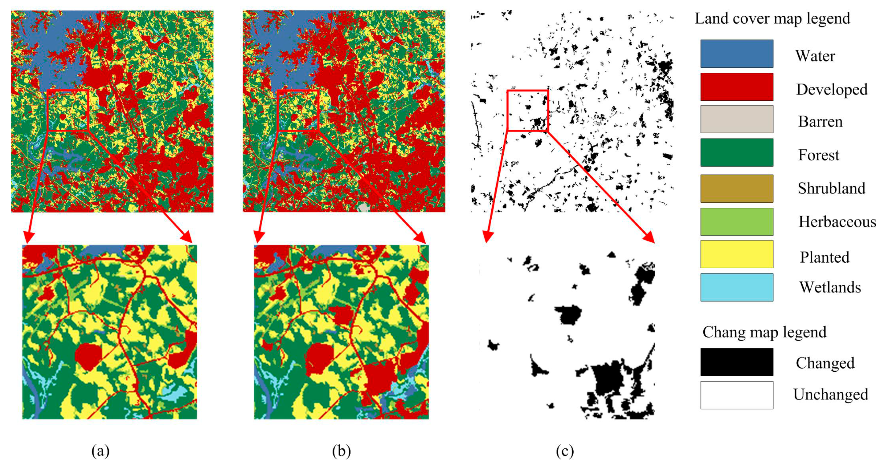
Figure 4.
National Land Cover Database (NLCD) land cover maps and the corresponding change maps in the study area: (a) NLCD 2001; (b) NLCD 2006; and (c) change map.
Figure 4.
National Land Cover Database (NLCD) land cover maps and the corresponding change maps in the study area: (a) NLCD 2001; (b) NLCD 2006; and (c) change map.

Figure 5.
Simulated coarse spatial resolution images for FCM_STSRM in experiment 1: (a) z = 4; (b) z = 8; and (c) z = 16.
Figure 5.
Simulated coarse spatial resolution images for FCM_STSRM in experiment 1: (a) z = 4; (b) z = 8; and (c) z = 16.

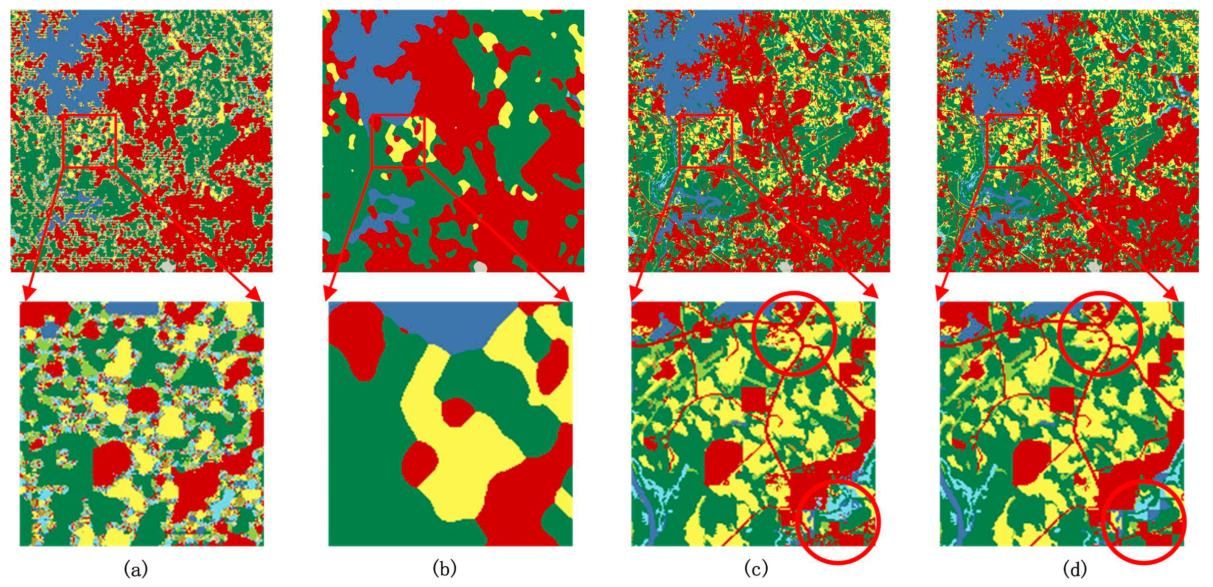
Figure 6.
Resultant land cover maps generated by the three different methods with different zoom factors: (a) HC (z = 4); (b) HC (z = 8); (c) HC (z = 16); (d) FCM_SRM (z = 4); (e) FCM_SRM (z = 8); (f) FCM_SRM (z = 16); (g) FCM_STSRM (z = 4); (h) FCM_STSRM (z = 8); and (i) FCM_STSRM (z = 16).
Figure 6.
Resultant land cover maps generated by the three different methods with different zoom factors: (a) HC (z = 4); (b) HC (z = 8); (c) HC (z = 16); (d) FCM_SRM (z = 4); (e) FCM_SRM (z = 8); (f) FCM_SRM (z = 16); (g) FCM_STSRM (z = 4); (h) FCM_STSRM (z = 8); and (i) FCM_STSRM (z = 16).

Figure 7.
The data used in experiment 2: (a) coarse resolution image (degraded image); (b) former finer-resolution land cover map; (c) latter finer-resolution land cover map (reference map); and (d) change map.
Figure 7.
The data used in experiment 2: (a) coarse resolution image (degraded image); (b) former finer-resolution land cover map; (c) latter finer-resolution land cover map (reference map); and (d) change map.

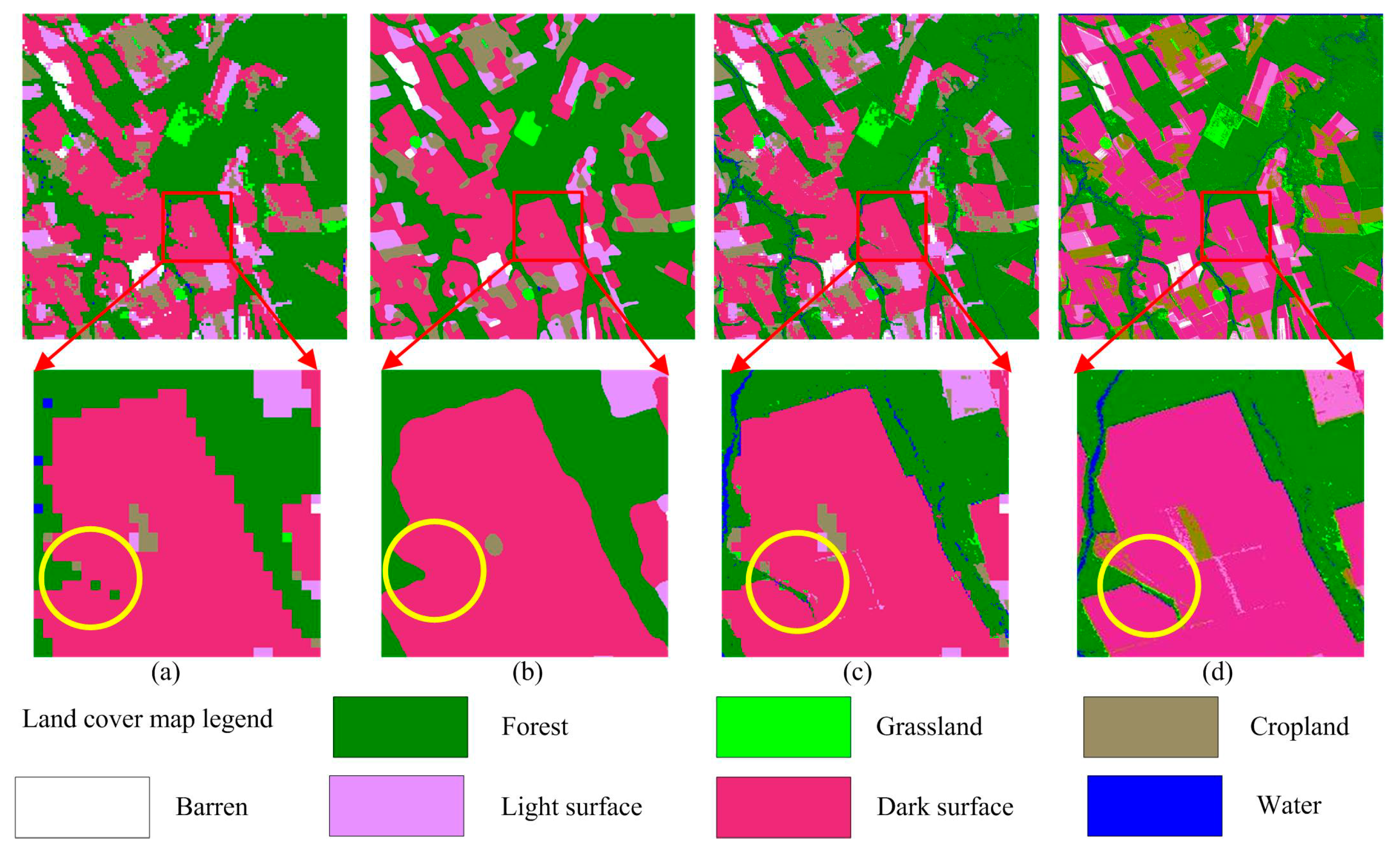
Figure 8.
Resultant land cover maps generated by different methods: (a) HC; (b) FCM_SRM; (c) FCM_STSRM; and (d) reference map.
Figure 8.
Resultant land cover maps generated by different methods: (a) HC; (b) FCM_SRM; (c) FCM_STSRM; and (d) reference map.

Figure 9.
Resultant land cover maps generated by FCM_STSRM with different weighting coefficients: (a) ; (b) ; (c) ; and (d) .
Figure 9.
Resultant land cover maps generated by FCM_STSRM with different weighting coefficients: (a) ; (b) ; (c) ; and (d) .

Figure 10.
Accuracy assessment of FCM_SRM and FCM_STSRM with different fuzziness parameters: (a) OA for FCM_SRM; (b) PULC for FCM_SRM; (c) PCLC for FCM_SRM; (d) OA for FCM_STSRM; (e) PULC for FCM_STSRM; and (f) PCLC for FCM_STSRM.
Figure 10.
Accuracy assessment of FCM_SRM and FCM_STSRM with different fuzziness parameters: (a) OA for FCM_SRM; (b) PULC for FCM_SRM; (c) PCLC for FCM_SRM; (d) OA for FCM_STSRM; (e) PULC for FCM_STSRM; and (f) PCLC for FCM_STSRM.


Table 1.
Accuracy statistics of different methods at different zoom factors.
| Zoom Factor | Methods | Kappa | OA | PULC | PCLC | KULC | KCLC |
|---|---|---|---|---|---|---|---|
| z = 4 | HC | 0.7638 | 83.14% | 82.89% | 85.89% | 0.7621 | 0.6808 |
| FCM_SRM | 0.7719 | 83.84% | 83.51% | 87.54% | 0.7691 | 0.7028 | |
| FCM_STSRM | 0.9640 | 97.41% | 98.41% | 86.04% | 0.9781 | 0.6903 | |
| z = 8 | HC | 0.6613 | 76.15% | 76.01% | 77.83% | 0.6616 | 0.5145 |
| FCM_SRM | 0.6650 | 76.20% | 77.83% | 79.92% | 0.6636 | 0.5385 | |
| FCM_STSRM | 0.9476 | 96.23% | 98.30% | 72.71% | 0.9765 | 0.4541 | |
| z = 16 | HC | 0.5630 | 69.65% | 69.76% | 68.29% | 0.5685 | 0.3385 |
| FCM_SRM | 0.5556 | 69.47% | 69.55% | 68.57% | 0.5615 | 0.3152 | |
| FCM_STSRM | 0.9240 | 94.53% | 98.22% | 52.48% | 0.9755 | 0.2100 |
Table 2.
Confusion matrix for the proposed FCM_STSRM in the entire area.
| Forest | Grassland | Cropland | Barren | Light Surface | Dark Surface | Water | |
|---|---|---|---|---|---|---|---|
| Forest | 551,605 | 16,172 | 7862 | 71 | 651 | 1250 | 14,892 |
| Grassland | 3349 | 17,037 | 1237 | 10 | 288 | 476 | 39 |
| Cropland | 2649 | 1743 | 98,027 | 142 | 3318 | 9187 | 434 |
| Barren | 182 | 103 | 547 | 17,355 | 2640 | 314 | 4 |
| Light surface | 936 | 787 | 6652 | 2519 | 76,752 | 4268 | 122 |
| Dark surface | 2653 | 2065 | 23,286 | 963 | 8396 | 368,894 | 708 |
| Water | 966 | 19 | 340 | 0 | 14 | 166 | 2310 |
Table 3.
Accuracy statistics of different methods.
| Methods | Kappa | OA | PULC | PCLC | KULC | KCLC |
|---|---|---|---|---|---|---|
| HC | 0.8293 | 88.52% | 94.78% | 82.43% | 0.7928 | 0.7303 |
| FCM_SRM | 0.8367 | 89.12% | 96.06% | 82.36% | 0.8386 | 0.7248 |
| FCM_STSRM | 0.8549 | 90.24% | 97.28% | 83.39% | 0.8879 | 0.7422 |
Table 4.
Accuracy statistics of the FCM_STSRM method with different weighting coefficients (%).
| Result Statistic | α | 0 | 0.001 | 0.01 | 0.1 | 1 | 10 | |
|---|---|---|---|---|---|---|---|---|
| β | ||||||||
| OA | 0 | 59.04 | 65.20 | 76.17 | 73.32 | 68.56 | 68.13 | |
| 0.001 | 80.99 | 82.53 | 80.56 | 73.66 | 68.54 | 68.21 | ||
| 0.01 | 95.90 | 96.32 | 95.65 | 76.59 | 69.16 | 68.28 | ||
| 0.1 | 96.13 | 96.23 | 96.23 | 95.66 | 73.68 | 68.48 | ||
| 1 | 96.13 | 96.17 | 96.17 | 96.18 | 95.63 | 73.31 | ||
| 10 | 96.13 | 96.17 | 96.17 | 96.17 | 96.17 | 95.63 | ||
| PULC | 0 | 59.07 | 65.05 | 75.85 | 73.21 | 68.70 | 68.25 | |
| 0.001 | 82.63 | 83.71 | 80.53 | 73.56 | 68.57 | 68.24 | ||
| 0.01 | 97.93 | 98.12 | 97.09 | 76.56 | 69.21 | 68.32 | ||
| 0.1 | 98.26 | 98.34 | 98.30 | 97.28 | 73.69 | 68.54 | ||
| 1 | 98.29 | 98.36 | 98.35 | 98.30 | 97.29 | 73.33 | ||
| 10 | 98.29 | 98.36 | 98.36 | 98.36 | 98.30 | 97.29 | ||
| PCLC | 0 | 58.68 | 66.90 | 79.71 | 74.58 | 67.04 | 66.81 | |
| 0.001 | 62.31 | 69.18 | 80.92 | 74.86 | 68.18 | 67.91 | ||
| 0.01 | 72.85 | 75.78 | 79.28 | 76.97 | 68.57 | 67.87 | ||
| 0.1 | 71.86 | 72.26 | 72.71 | 77.23 | 73.62 | 67.89 | ||
| 1 | 71.65 | 71.33 | 71.40 | 72.01 | 76.82 | 73.13 | ||
| 10 | 71.58 | 71.29 | 71.30 | 71.32 | 71.94 | 76.78 | ||
© 2018 by the authors. Licensee MDPI, Basel, Switzerland. This article is an open access article distributed under the terms and conditions of the Creative Commons Attribution (CC BY) license (http://creativecommons.org/licenses/by/4.0/).
Share and Cite
MDPI and ACS Style
Yang, X.; Xie, Z.; Ling, F.; Li, X.; Zhang, Y.; Zhong, M. Spatio-Temporal Super-Resolution Land Cover Mapping Based on Fuzzy C-Means Clustering. Remote Sens. 2018, 10, 1212. https://doi.org/10.3390/rs10081212
AMA Style
Yang X, Xie Z, Ling F, Li X, Zhang Y, Zhong M. Spatio-Temporal Super-Resolution Land Cover Mapping Based on Fuzzy C-Means Clustering. Remote Sensing. 2018; 10(8):1212. https://doi.org/10.3390/rs10081212
Chicago/Turabian StyleYang, Xiaohong, Zhong Xie, Feng Ling, Xiaodong Li, Yihang Zhang, and Ming Zhong. 2018. "Spatio-Temporal Super-Resolution Land Cover Mapping Based on Fuzzy C-Means Clustering" Remote Sensing 10, no. 8: 1212. https://doi.org/10.3390/rs10081212
Note that from the first issue of 2016, this journal uses article numbers instead of page numbers. See further details here.