Improving the Estimation of Daily Aerosol Optical Depth and Aerosol Radiative Effect Using an Optimized Artificial Neural Network

Abstract

Aerosols can absorb and scatter surface solar radiation (SSR), which is called the aerosol radiative forcing effect (ARF). Great efforts have been made for the estimation of the aerosol optical depth (AOD), SSR and ARF using meteorological measurements and satellite observations. However, the accuracy, and spatial and temporal resolutions of these existing AOD, SSR and ARF models should be improved to meet the application requirements, due to the uncertainties and gaps of input parameters. In this study, an optimized back propagation (BP) artificial neural network (Genetic_BP) was developed for improving the estimation of the AOD values. The retrieved AOD values using the Genetic_BP model and meteorological measurements at China Meteorological Administration (CMA) stations were used to calculate SSR and bottom of the atmosphere (BOA) ARF (ARFB) using Yang’s Hybrid model (YHM). The result show that the Genetic_BP could be used for estimating AOD values with high accuracy (R = 0.866 for CASNET (China Aerosol Remote Sensing Network) stations and R = 0.865 for AERONET (Aerosol Robotic Network) stations). The estimated SSR also showed a good agreement with SSR measurements at 96 CMA radiation stations, with RMSE, MAE, R and R² of 29.27%, 23.77%, 0.948, and 0.899, respectively. The estimated ARFB values are also highly correlated with the AERONET ARFB ones with RMSE, MAE, R and R² of −35.47%, −25.33%, 0.843, and 0.711, respectively. Finally, the spatial and temporal variations of AOD, SSR, and ARFB values over Mainland China were investigated. Both AOD and SSR values are generally higher in summer than in other seasons. The ARFB are generally stronger in spring and summer than in other seasons. The ranges for the monthly mean AOD, SSR and ARFB values over Mainland China are 0.183–0.333, 10.218–24.196 MJ m⁻²day⁻¹ and −2.986 to −1.244 MJ m⁻²day⁻¹, respectively. The Qinghai-Tibetan Plateau has always been an area with the highest SSR, the lowest AOD and the weakest ARFB. In contrast, the Sichuan Basin has always been an area with low SSR, high AOD, and strong ARFB. The newly proposed AOD model may be of vital importance for improving the accuracy and computational efficiency of AOD, SSR and ARFB estimations for solar energy applications, ecological modeling, and energy policy.

1. Introduction

Solar radiation (SSR) is defined as the power per unit area received from the Sun in the form of electromagnetic radiation [1]. SSR is composed of direct and diffuse solar radiation, which controls the sources and sinks of energy between the Earth surface and atmosphere [2]. It is also an indispensable term in biological and physical processes such as evapotranspiration [3], chlorophyll synthesis [4], and plant photosynthesis [5]. Solar radiation can be directly absorbed and scattered by aerosol, which is called the aerosol radiative forcing effect (ARF) [6]. The aerosol optical depth (AOD) is the key aerosol parameter, which would significantly affect the quality of ARF estimations. Many ground-based remote sensing aerosol networks have been established around the world, for example the Aerosol Robotic Network (AERONET) can provide continuous cloud-screened observations of spectral AOD values around the world [7]. In China, AOD values are routinely measured at about 50 sites of the China Aerosol Remote Sensing Network (CARSNET) over Mainland China [8]. However, the sites of AERONET and CARSNET are relatively sparse for AOD applications requiring high spatial resolutions. Remote sensing provides an efficient way to retrieve spatiotemporally continuous AOD values at regional and global scales. The Total Ozone Mapping Spectrometer (TOMS) aboard Nimbus-7 (1976–1992) and Earth Probe Satellite (1996 to present) can provide long-term AOD records around the world [9]. Torres et al. [9] found that the AOD values for UV-absorbing conditions derived from TOMS are within 30% of the AERONET observations, while the AOD values for non-absorbing conditions are within 20% of the AERONET observations. Nevertheless, the nadir spatial resolutions (about 50 km × 50 km) of TOMS are relatively coarse for AOD applications. The Advanced Along Track Scanning Radiometer (AATSR) aboard Envisat can also provide AOD products with high nadir spatial resolution (1 km × 1 km) [10]. Meanwhile, the Seaviewing Wide Field-of-view Sensor (SEAWIFS) aboard GeoEye’s OrbView-2 can provide AOD data on global ocean with spatial resolution of 9 km×9 km [11]. Long term daily and monthly AOD records (1981–2017) can also be obtained from the Advanced Very High Resolution Radiometer (AVHRR) aboard on TIROS-N and NOAA series with nadir spatial resolution of 1.1 km × 1.1 km [12]. Among all AOD products, the standard AOD products from the Moderate Resolution Imaging Spectroradiometer (MODIS) on board Terra and Aqua are the most widely used AOD products for the estimation of AOD, with spatial resolutions of 3 km and 10 km, respectively. However, the accuracies, the spatial and temporal continuities, and the spatial and temporal resolutions of these above AOD products should be improved.

Numerous models have been developed for estimating AOD values using meteorological measurements and satellite observations. Empirical models assume that AOD is a synergy consequence of meteorological parameters such as sunshine duration, air temperature, relative humidity, visibility, cloud fraction and elevation [13,14,15,16,17,18,19]. However, empirical models are inflexible to the natural environment, due to ignoring the physical processes and terrain effects. Moreover, these models are subject to the meteorological network is quite dense worldwide in contrast to the solar radiation one. Satellite observations provide an efficient way to retrieve spatiotemporally continuous AOD values at regional and global scales [20,21,22,23,24]. Both geostationary satellites and polar orbiting satellites can provide essential atmospheric and land surface information with different spatial and temporal resolutions. Numerous models have been developed for estimating AOD using satellite observations [23,25,26,27,28,29,30,31]. Despite the effectiveness and superiority of satellite-based AOD models, the accuracy of satellite retrievals is subject to many uncertainties such as calibration, cloud screening, aerosol model and surface reflection. Meanwhile, artificial intelligence (AI) is a new and promising approach for retrieving AOD with high accuracy. Many artificial neural network (ANN) models have been developed to retrieve AOD in regional and global scales [32,33,34]. Lanzaco et al. [35] integrated ANN and support vector machine (SVM) to obtain AOD values. The result showed that the estimated AOD values showed better accuracy than MODIS AOD products. However, this model was subjected to the short time series of MODIS products (starting 2001). Huttunen et al. [36] made a comparative study on the model accuracy of transfer-based look-up table, non-linear regression and machine learning algorithms for predicting AOD values. The result indicated that the estimated AOD values by ANN and SVM showed good agreement with AERONET measurements. More meteorological parameters such as wind speed, visibility and relative humidity which were highly correlated with AOD could be incorporated into AI models to improve the accuracy of AI models. Furthermore, some intrinsic drawbacks of AI models such as the slow convergence speed and the intrinsic disadvantages of revealing the relative significance of input parameters would degrade the accuracy of AI methods. Many optimization models such as Genetic algorithm [37] could be used to optimize the weights and the thresholds of the BP neural network for the estimation of AOD values.

Strong ARF was observed around the world, and it varies regionally as a result of precipitation, humidification, and other hydrological processes [38]. The ARF has become one of the most uncertain factors affecting global climate change, and one hot topic in the global climate change research [39]. Kirkevagand Iversen [40] calculated the global aerosol radiation effect during 2000–2100 using the Community Climate Model (CCM3.2) based on the climate scenario (2000–2100) proposed by Intergovernmental Panel on Climate Change (IPCC). The results indicated that the global ARF caused by black carbon aerosol in 2000 and 2100 were about −0.11 Wm⁻² and 0.11 Wm⁻², respectively. Ma et al. [41] reconstructed global ARF values at the top of the atmosphere (ARF_TOA) using GEOS-Chem-APM climate models, the results showed that the global ARF_TOA is about −0.41 Wm⁻². Myhre et al. [42] made a comparative study on the model performances of 16 climate models for the estimation of global ARF. The results indicated that the global ARF is about −0.27 Wm⁻² (−0.58 to −0.02 Wm⁻²). According to the sources of aerosol particles, the ARF could be roughly divided into the natural ARF and the anthropogenic one [43]. Dust is the main source to the natural aerosol particles in the atmosphere, especially in desert and arid areas. Li et al. [44] reconstructed the ARF of the Sahara Desert using the aerosol and solar radiation observations of the MODIS satellite products and CERES (Clouds and Earth’s Radiant Energy). The results indicated that the monthly mean ARF_TOA in summer was 26 ± 3 Wm⁻², which was significantly stronger than that in other months. Sea salt particulates are the main causes of the global marine ARF, and exert great cooling effect on the global ocean [45]. Lee et al. [46] proposed a model for estimating aerosol optical properties and aerosol radiative forcing effect using satellite data. The spatial and temporal variations of the ARF_TOA in the global ocean were analyzed. The results showed that the ARF_TOA and ARFB over the global ocean were −5.2 ± 0.5 and 8.3 Wm⁻², respectively. Since the industrial revolution, the anthropogenic aerosol emissions have shown an explosive growth trend, resulting in significant radiation forcing effects on solar radiation [43]. The black carbon aerosol particles, the organic carbon aerosol particles and the sulfate aerosol particles are the main anthropogenic aerosol particles [47]. Many climate model including the Beijing Climate Center atmospheric general circulation model (BCC_AGCM2.0.1) and the Canadian Aerosol Module (CAM) [48], ACCMIP (Atmospheric Chemistry & Climate Model Intercomparison Project), EDGAR-HTAP (Emission Database for Global Atmospheric Research for Hemispheric Transport of Air Pollution), and EDGAR Version 4.2, and one regional INTEX-B (Intercontinental Chemical Transport Experiment—Phase B) inventory [49], Coupled Model Intercomparison Project (CMIP5/CMIP6) [50], chemistry-transport model (CTM) [51], The European Monitoring and Evaluation Programme (EMEP) [52], global chemical transport model (GEOS-Chem) [53,54,55], GFDL AM2 GCM [56], Goddard Global Ozone Chemistry Aerosol Radiation and Transport (GOCART) [57], Laboratoire de Météorologie Dynamique General Circulation Model (LMDZ) [58], Modtran (MODerate resolution atmospheric TRANsmission) [59], the Scripps Monte-Carlo Aerosol Cloud Radiation (MACR) [60], SBDART (Santa Barbara DISORT Atmospheric Radiative Transfer) [61], SPRINTARS (Spectral Radiation-Transport Model for Aerosol Species) [62], and WRF (Weather Research and Forecasting) [63] have been applied for analyzing the anthropogenic ARF in regional and global scales. However, the computational efficiency of these climate models needs further improvement.

Great efforts have been made for estimating AOD and ARF throughout China. Zhang et al. [64] analyzed the spatial and temporal variations of AOD values during 1973–2014 using the KM-Elterman method. The results showed that the estimated AOD values were in good agreement with the AOD values derived from MODIS products (R = 0.942). The North China Plain, the Yangtze River Delta, central China, the Sichuan Basin, and the Pearl River Delta were the areas with rapidly increasing trend of AOD values; the southwest China was found to be an area with significant decreasing trend of AOD values. Xu et al. [65] reconstructed the AOD values during 1993–2012 throughout China using a broadband extinction model, which showed good agreement with AERONET AOD values with RMSE, MAE and R of 0.101, 0.029 and 0.848, respectively. Guo et al. [66] revealed the spatial and temporal characteristics of the AOD values during 1980–2008 over Mainland China using TOMS AOD (1980–2001) and MODIS AOD products (2000–2008). Meanwhile, many studies have been conducted at regional scale in China using meteorological measurements and satellite observations [67,68,69,70,71]. China is a big country with severe anthropogenic aerosol emissions, which has posed great uncertainties on the global climate change. Many studies have been conducted on the spatial and temporal variations of the aerosol radiative effect in China. These studies were mainly focused on the area with intensive population and air pollution, for example Central-East China [72], the Pearl River Delta [73], and the Yangtze River Delta [8]. However, few studies have been made for analyzing the AOD and ARF values in different climate zones and terrain features over Mainland China, due to the relative sparse AOD and SSR measurements in China. Further studies should be made on the spatial and temporal variations of AOD and the ARF on SSR over Mainland China.

This study attempted: (1) to explore a new simplified model (Genetic_BP) for improving the estimation of AOD, SSR and ARFB values, based on the Genetic algorithm, back propagation neural network (BP) and an SSR estimation model (hereafter, YHM) developed by Yang et al. [74]; (2) to evaluate the retrieved AOD values by the Genetic_BP model and the retrieved SSR and ARF values by YHM in various climate zones throughout China using daily AOD, SSR, ARF measurements; and (3) to reveal the spatial and temporal variations of AOD, SSR and ARFB values in different climate zones and terrains over Mainland China.

2. Materials and Methods

2.1. Study Area and Data

2.1.1. Observation Data

Daily AOD (550 nm) records during 2002–2014 at CARSNET and AERONET stations throughout China were used for the estimation and validation of AOD values. Then, these AOD retrievals together with daily meteorological measurements including air temperature (T), relative humidity (RH), surface pressure (P), and sunshine duration (SH) at 839 CMA stations were used to retrieve SSR and ARFB over Mainland China using the YHM model. Finally, daily SSR measurements at 96 CMA stations (2002–2014) and the aerosol radiative effect (bottom of atmosphere) data at AERONET observations (2002–2014) were used for validating the accuracy of the SSR and ARFB retrievals by the YHM model, respectively. Figure 1 shows the spatial distribution of these CARSNET stations, AERONET stations, SSR stations, CMA meteorological stations and AERONET stations.

Table 1. Geographical and annual mean meteorological data at CARSNET, AERONET, SSR and CMA stations.

Network of Stations	Statistics	Lat (deg)	Lon (deg)	A (m)	P (hpa)	RH	SH (h)	T (°C)
CARSNET	max	47.73°N	126.77°E	3648.9	1042.1	1.00	14.60	35.70
	min	22.63°N	79.93°E	2.5	638.9	0.05	0.00	−33.10
	mean	-	-	856.9	922.7	0.56	6.59	11.49
	std	-	-	956.7	99.1	0.21	4.11	12.06
AERONET	max	42.68°N	122.70°E	4276.0	1046.2	0.97	14.00	34.60
	min	22.21° N	86.95°E	0	592.4	0.08	0.00	−20.80
	mean			827.4	958.7	0.52	8.52	9.95
	std			1194.4	113.3	0.17	2.66	11.38
SSR	max	52.97°N	130.3°E	4507.0	1048.7	1.00	15.70	38.90
	min	18.22°N	75.98°E	2.5	573.5	0.05	0.00	−39.80
	mean	-	-	900.7	919.0	0.61	6.29	11.94
	std	-	-	1111.8	111.4	0.20	4.11	12.46
CMA	max	52.58°N	132.58°E	4507.0	1048.7	1.00	15.70	38.90
	min	16.50°N	75.14°E	1.3	558.4	0.04	0.00	−44.60
	mean	-	-	979.2	911.3	0.63	6.14	11.47
	std	-	-	1116.7	117.4	0.20	4.07	12.47

Lat is latitude, Lon is longitude, A is altitude above sea level, P is surface pressure, RH is relative humidity (100%), SH is sunshine duration, T is air temperature.

shows the statistical indicators representing the geographical and climate patterns of these CARSNET, AERONET, SSR and CMA stations. These stations cover most areas of China with various and complicated geomorphology and terrain features.

Figure 2 shows the monthly variations of T, RH, P, and SH for CARSNET, AERONET, SSR and CMA stations. T was generally higher in summer and lower in winter. The highest monthly mean T for CARSNET, AERONET, SSR and CMA were 24.91 °C, 26.08 °C, 24.43 °C and 23.72 °C in July, respectively. The lowest monthly mean T for CARSNET, AERONET, SSR and CMA were −4.78 °C, −3.52 °C, −3.27 °C and −3.41 °C in January, respectively. The P for CARSNET, AERONET, SSR, and CMA were generally higher in winter and lower in summer. The highest monthly mean P for CARSNET (930.91 hPa), AERONET (930.91 hPa), SSR (926.62 hPa), and CMA (918.26 hPa) were in January; and the lowest monthly mean P for CARSNET (913.91hPa), AERONET (913.91 hPa), SSR (911.04 hPa), and CMA (903.99 hPa) were in July. The highest monthly mean RH for CARSNET (65.51%), AERONET (67.51%), SSR (67.47%) and CMA (69.40%) were in September; and the lowest monthly mean RH for CARSNET (45.99%), AERONET (40.55%), SSR (52.78%) and CMA (55.65%) were in April. The SH were generally higher in spring and summer and lower in winter. The longest monthly mean SH for CARSNET (7.94 h), AERONET (10.25 h), SSR (7.27 h) and CMA (7.04 h) were in June, May, May, and August, respectively; and the shortest monthly mean SH for CARSNET (5.36 h), AERONET (6.89 h), SSR (5.13 h) and CMA (5.15 h) were in February, December, January and January, respectively.

2.1.2. MODIS Products and MERRA2 Datasets

The AOD values derived from MODIS level-2 products (MOD04/MYD04) and level-3 products (MOD08/MYD08) during 2002–2014 were validated at CARSNET and AERONET stations in this study. Meanwhile, the daily mean AOD values derived from MERRA2 (The Modern Era Retrospective-Analysis for Research and Applications) during 1980–2015 were also evaluated using AOD measurements from CARNET and AERONET stations.

2.1.3. Climatic Zones and Terrain Features

The Shuttle Radar Topography Mission (SRTM) 90m digital elevation model (DEM) data were used to derive surface elevation (http://srtm.csi.cgiar.org/SELECTION/inputCoord.asp). The climate and terrain regionalization data were provided by Resource and environment science data center of the Chinese Academy of Sciences (http://www.resdc.cn). Figure 3 shows the terrain features in China. There are 50 topographic zones over Mainland China.

2.2. Optimized Back Propagation Neural Network Based on Genetic Algorithm

The back propagation (BP) neural network is the most widely used AI models for numerical fitting problems with strong learning ability and high accuracy [75]. The basic idea of BP is to find a function that best maps a set of input parameters to the correct output values using gradient descent optimization algorithm, which minimizes the mean square error between the network’s actual output value and the expected output value [76]. In this study, nine parameters (RH, T, P, SD, A, day number (D), visibility (VIS) and cloud fraction (TCP), and MERRA2 AOD) that were closely correlated with AOD values were set as input parameters for the BP model; daily AOD measurements at the CARSNET and AERONET stations were set as the model output parameter for the BP model. A total of 70% of the databases during the whole study period were used to train the BP model, and 30% of them were used for testing the model. The AOD values could be calculated using the following equation:

$${\mathrm{F}}_{\mathrm{g}}=\mathrm{Z}\left({\displaystyle \sum }_{\mathrm{i}=1}^{\mathrm{N}}{\mathrm{w}}_{\mathrm{i}}\left(\mathrm{t}\right){\mathrm{x}}_{\mathrm{i}}\left(\mathrm{t}\right)+\mathrm{b}\right)$$

(1)

where F_g is the estimated AOD; Z (w, x, b) means the hidden transfer function; w_i (t) is the weight; x_i(t) is the input parameter indiscrete time space; and b is the neuronal bias. The basic schematic architecture of the BP neural network in this study is illustrated in Figure 4.

Then, the Genetic algorithm was introduced to optimize the weights and the thresholds of the BP neural network for the estimation of AOD values. It is a meta-heuristic algorithm proposed by Holland [37] inspired by the process of natural selection that belongs to the larger class of evolutionary algorithms, which is commonly used to generate high-quality solutions to optimization and search problems. The Genetic_BP model for improving the estimation of AOD values could be conducted as the following steps (Figure 5):

(1)

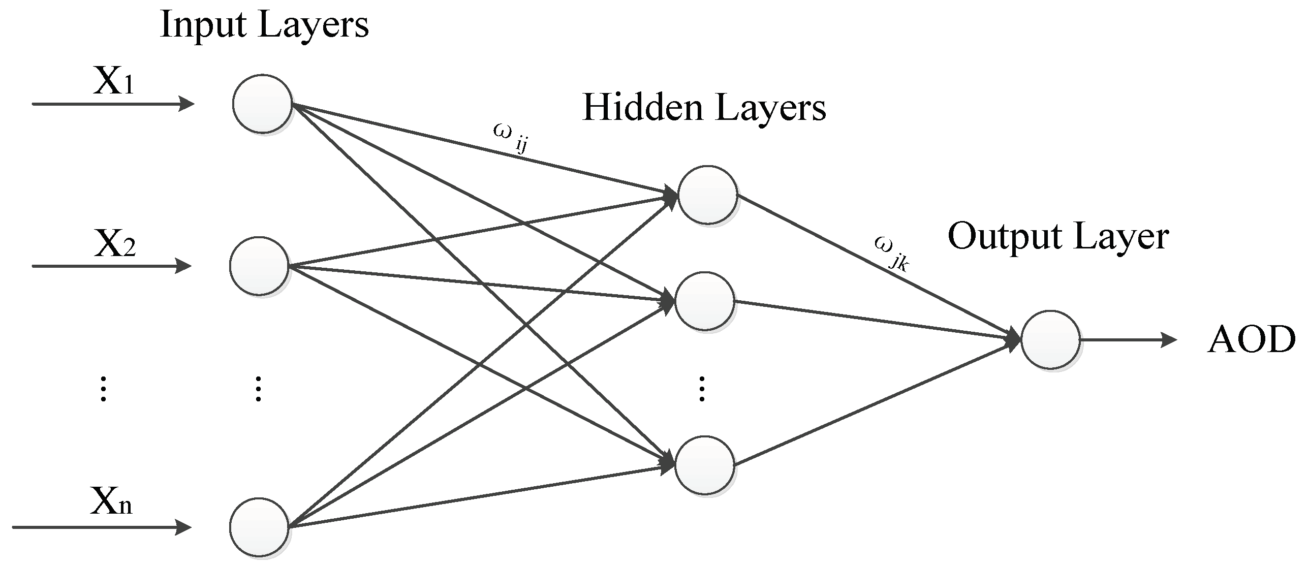
Initialize random population. The basic structure of the BP neural network in this study is 9-10-1 (Figure 4) with 9 input layers, 10 hidden layers and 1 output layer. Thus, the number of weights is 9 × 10 + 10 × 1 = 100; the number of thresholds is 10 + 1 = 11. Thus, the encoding length is 100 + 11 = 111.

(2)

Selection operation. The new individuals with high fitness values would be selected from old individuals using roulette selection method. The selection probability for individuals was calculated as following equation:

$$g_i=a/S_i$$

(2)

$$P_i=g_i/{\displaystyle \sum }_{j=1}^n{g}_i$$

(3)

where $P_i$ is the selection probability; and $g_i$ is the fitness value, which could be calculated as follows:

$$S_i=b({\displaystyle \sum }_{j=1}^{N}abs(y_i-o_i))$$

(4)

where N is the number of the input layers of BP neural network (6); y_i is the i-th expected output value; o_i is the i-th predicted output values; and b is a constant value.

(3)

Crossover operation. The crossover operation was conducted using arithmetic crossover algorithm:

$$\begin{array}{c}{a}_{cj}=a_{cj}\left(1-b\right)+a_{dj}b\\ a_{dj}=a_{dj}\left(1-b\right)+a_{cj}b\end{array}\}$$

(5)

where $a_{cj}$ and $a_{dj}$ are the c-th and d-th chromosome at j position; and b is a constant within 0–1.

(4)

Mutation operation. The mutation operation was conducted using following equations:

$$a_{ij}=\{\begin{array}{c}{a}_{ij}+\left(a_{ij}-a_{max}\right)\ast f\left(g\right)r>0.5\\ a_{ij}+\left(a_{min}-a_{ij}\right)\ast f\left(g\right)r\le 0.5\end{array}$$

(6)

$$f\left(g\right)=r_2{\left(1-g/G_{max}\right)}^2$$

(7)

where a_max and a_min are the maximum and minimum value for a_ij; r is a random number [0–1]; r₂ is also random number; g is the number of iterations; and Gmax is maximum evolution times. Detailed information about the Genetic_BP model can be found in [77].

2.3. Yang’s Hybrid Model

Yang’s Hybrid model (YHM) is a physically-based broadband model for estimating solar radiation, taking into account of five main radiation-damping processes, including Rayleigh scattering, aerosol extinction, ozone absorption, water vapor absorption and gas absorption. YHM was first developed by Yang et al. [78], then improved by Yang and Koike [79] for hydrological applications, and further improved by Yang et al. [74] by importing global data sets. YHM is recognized as one of the best SSR models [80,81], which could be expressed as follows:

$$H_{all}={\tau }_c{H}_{clr}$$

(8)

where $H_{all}$ means the daily surface solar radiation (MJ m⁻²day⁻¹) for all-sky conditions. The cloud effect on daily SSR is corrected using a cloud transmittance parameter ${\tau }_c$, which is a function of the actual sunshine durations (SH) and the maximum possible sunshine durations (N). Detail description on Yang’s Hybrid model could be found in Appendix A.

2.4. Aerosol Radiative Forcing Effect on SSR

The ARF is defined here as [82]:

$$ARF=SS{R}_{NA}-SS{R}_{WA}$$

(9)

where $SS{R}_{WA}$ is the estimated SSR without the presence of aerosols in the atmosphere; and $SS{R}_{NA}$ denotes the estimated SSR with aerosols in the atmosphere.

2.5. Model Performance

The following statistical indicators including the correlation coefficient (R), the determination coefficient (R²), the mean absolute bias error (MAE, %), the root mean square error (RMSE, %), and the root mean square error value (RMSEE, MJ m⁻²day⁻¹) were used to evaluate the model accuracy for the Genetic_BP model and the YHM solar radiation model:

$$R=\frac{{\displaystyle {\sum }_{i=1}^n(G_{est,i}-\overline{G_{est,i}})(G_{obs,i}-\overline{G_{obs,i}})}}{\sqrt{{\displaystyle {\sum }_{i=1}^n{(G_{obs,i}-\overline{G_{obs,i}})}^2}}\sqrt{{\displaystyle {\sum }_{i=1}^n{(G_{est,i}-\overline{G_{est,i}})}^2}}}$$

(10)

$$R^2={\left(\frac{{\displaystyle {\sum }_{i=1}^n(G_{est,i}-\overline{G_{est,i}})(G_{obs,i}-\overline{G_{obs,i}})}}{\sqrt{{\displaystyle {\sum }_{i=1}^n{(G_{obs,i}-\overline{G_{obs,i}})}^2}}\sqrt{{\displaystyle {\sum }_{i=1}^n{(G_{est,i}-\overline{G_{est,i}})}^2}}}\right)}^2$$

(11)

$$RMSE=100/\overline{M}\times \sqrt{({\displaystyle {\sum }_{i=1}^n{(G_{obs,i}-G_{est,i})}^2})/n}$$

(12)

$$MAE=100/\overline{M}\times ({\displaystyle {\sum }_{i=1}^n\left|G_{obs,i}-G_{est,i}\right|})/n$$

(13)

$$RMSEE=\sqrt{({\displaystyle {\sum }_{i=1}^n{(G_{obs,i}-G_{est,i})}^2})/n}$$

(14)

where n means the number of data points; $G_{est,i}$ and $G_{obs,i}$ are the estimated and observed AOD/ARF/SSR, respectively; $G_{est,i}$ and $G_{obs,i}$ represent the mean of the estimated AOD/ARF/SSR and observed AOD/ARF/SSR, respectively; and $\overline{M}$ means the mean of the observed AOD/ARF/SSR values.

3. Results and Discussion

3.1. Validation of Estimated AOD

The AOD values retrieved by the Genetic_BP model were directly compared with measured AOD values at the CARSNET and AERONET stations. Figure 6a shows the scatter plot of AOD values from the CARSNET stations and AOD values calculated by Genetic_BP. Figure 6b shows the scatter plot of AOD values from the AERONET stations and AOD values calculated by the Genetic_BP. The results show that estimated AOD values by the Genetic_BP model have comparable accuracy. A very strong positive correlation between the estimated AOD values and CASNET/AERONET AOD ones is observed with small estimation errors. The RMSE, MAE, R and R² for the estimated AOD values at the CARSNET stations are 41.46%, 27.51%, 0.866 and 0.749, respectively. The RMSE, MAE, R and R² for the estimated AOD values at the AERONET stations are 44.98%, 29.23%, 0.865 and 0.747, respectively.

Figure 7 shows the monthly variations of the statistical indicators representing the model accuracy of the Genetic_BP models at the CARSNET stations and AERONET stations, respectively. The results show that the model deviations for Genetic_BP model were relatively large in summer than that in spring and winter, due to the effect of cloudy and rainy weather in summer on the ground meteorological measurements. The largest RMSE (45.56%) and MAE (29.94%) for the estimated AOD values at CARSNET stations were found in September; the smallest RMSE (34.74%) and MAE (24.49%) were found in December; the smallest R (0.847) and R² (0.718) were in December; and the largest R (0.887) and R² (0.787) in September. The largest RMSE (59.76%) and MAE (39.66%) for the estimated AOD values at the AERONET stations were found in July; the smallest RMSE (44.80%) and MAE (29.82%) were found in October; the smallest R (0.801) and R² (0.642) were in May; and the largest R (0.875) and R² (0.766) were in December.

The AOD retrievals by the Genetic_BP model were also compared with the AOD observations and estimations from MODIS and MERRA2 atthe CARSNET stations. Figure 8 illustrates the performance of the AOD values derived from five MODIS AOD products including MOD08/MYD08 Deep Blue algorithm (MODIS08DB), MOD08/MYD08 Combined Deep Blue and Dark Target algorithm (MODIS08DTBC), MOD08/MYD08 Mean values (MODIS08MEAN), MOD04/MYD04 Deep Blue algorithm (MODIS04DB), MOD04/MYD04 Dark Target algorithm (MODISDT). Figure 8f presents the scatter plot between the AOD values derived from MERRA2 AOD datasets and CARSNET AOD values. The AOD retrievals using the Genetic_BP model performs superior to the MODIS AOD and MERRA2 AOD products. The RMSE for MODIS08DB, MODIS08DTBC, MODIS08MEAN, MODIS04DB, MODIS04DT and MERRA-2 AOD were 73.85%, 74.34%, 82.16%, 69.15%, 68.20% and 61.89%, respectively; the MAE values were50.84%, 50.35%, 55.48%, 47.28%, 46.82% and 39.36%, respectively; the R were 0.666, 0.679, 0.697, 0.706, 0.758 and 0.705, respectively; and the R² were 0.444, 0.461, 0.486, 0.499, 0.575 and 0.497 respectively. Overall, the accuracy of the AOD values derived from MODIS and MERRA2 is relatively poor. Therefore, the Genetic_BP model can be used for estimating AOD values over Mainland China with high accuracy.

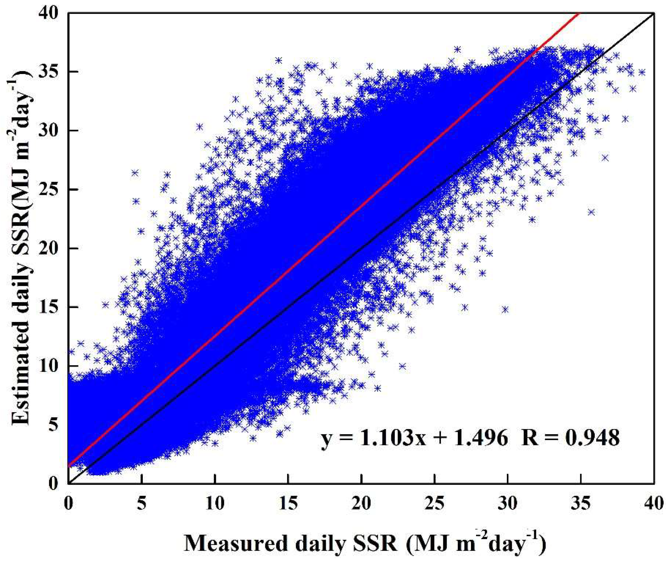
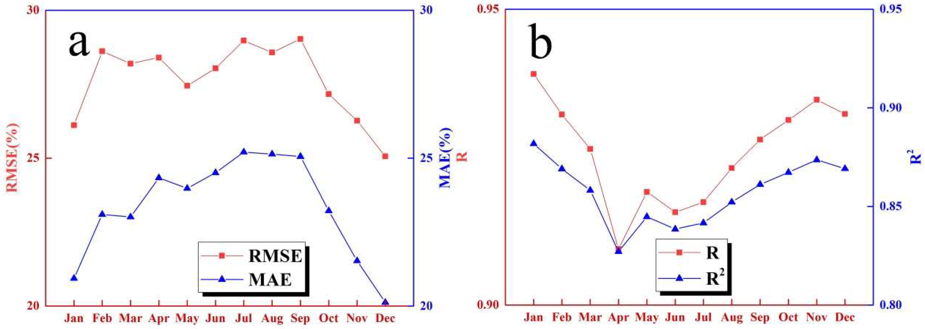
3.2. Validation of the Estimated SSR

Daily AOD values retrieved by the Genetic_BP model and meteorological measurements at 96 CMA radiation stations over Mainland China were used for the estimation of SSR using YHM. Figure 9 shows the validation result of the estimated SSR values by YHM at 96 CMA radiation stations. The results show that the YHM can estimate the SSR values with high accuracy, with RMSE, MAE, R and R² of 29.27%, 23.77%, 0.948 and 0.899, respectively. Figure 10 illustrates the spatial distributions of RMSE and MAE for YHM throughout China, respectively. It is clear that the YHM shows comparable performance over Mainland China, especially in the Plateau zones due to its strict theoretical basis on the radiation dumping processes in the atmosphere; for example, the RMSE for Ganzi, Germu, Gangcha and Lhasa were 8.36%, 8.51%, 9.63% and 9.65%, respectively; and the MAE were 6.74%, 7.00%, 7.66% and 7.88%, respectively. The model accuracy in northern China is generally higher than that in southern China, due to the dry air conditions there; for example, the RMSE for Erenhot, Ejinaqi and Urat in Inner Mongolia were 8.90%, 9.18% and 9.88%, respectively; and the MAE were 5.91%, 6.45% and 6.88%, respectively. Relatively larger estimation errors mainly distributed in southern China, owing to the abundant precipitable water vapor, changing weather and frequent cloud occurrence there; for example, the RMSE for Jishou in Hunan province, Ganzhou in Jinagxi province and Changsha in Hunan province were 30.55%, 29.25% and 27.52%, respectively; the MAE are 25.36%, 23.25% and 23.18%, respectively. The largest estimation errors were found in Chongqing in the Sichuan Basin, with RMSE and MAE of 35.95% and 30.11%, respectively, while the smallest estimation errors were found in Gaer in the Tibetan Plateau, with RMSE and MAE of 6.87% and 5.16%, respectively.

Figure 11 shows the monthly variation of the RMSE, MAE, R and R² for YHM over Mainland China. The results show that the YHM performs superior in autumn and winter than that in summer and spring, owing to the relatively larger estimation error of the AOD retrievals in spring and the frequent cloudy and rainy days and changing weather in summer. The largest RMSE (29.02%) and MAE (25.13%) for YHM are found in September and August, respectively, while the smallest RMSE (25.06%) and MAE (20.12%) in December. The smallest R (0.909) and R² (0.827) were in April, while the largest R (0.934) and R² (0.873) were in January.

The SSR retrievals by the YHM model were compared with other SSR estimates from previous studies. Yang et al. [78] developed a hybrid model (YHM) for estimating SSR, and validated at the Germu station in Qinghai-Tibetan Plateau with RMSEE and R of 2.86 MJm⁻²day⁻¹ and 0.96, respectively. Yang et al. [78] also evaluated the performance of the calibrated Angstrom model at the Germu station with RMSEE and R of 2.99 MJm⁻²day⁻¹ and 0.96, respectively. Our retrievals from the Germu station in this study perform superior than the estimated SSR values using YHM in previous studies with RMSEE and R of 2.77 MJm⁻²day⁻¹ and 0.96, respectively. Qin et al. [83] made a comparative study of the performance of four SSR models over Mainland China, including the YHM, EPP, an hourly solar radiation model (HSRM) and an artificial neutral network model (ANNM). The results show that the YHM has better performances than EPP, HSRM, and ANNM. The RMSEE for YHM, EPP, HSRM, and ANNM were 2.40 MJm⁻²day⁻¹, 2.41 MJm⁻²day⁻¹, 2.53 MJm⁻²day⁻¹, 3.64 MJm⁻²day⁻¹, and 2.85 MJm⁻²day⁻¹, respectively; the R for YHM, EPP, HSRM, and ANNM were 0.94, 0.91, 0.91, 0.81, and 0.88, respectively. Qin et al. [84] evaluated the accuracy of three SSR products including ISCCP-FD, GEWEX-SRB, and GLASS products over Mainland China. The results indicated that the SSR retrievals by YHM were more accurate than those from the ISCCP-FD, GEWEX-SRB, and GLASS products. The RMSEE for ISCCP-FD, GEWEX-SRB, and GLASS were 2.40 MJm⁻²day⁻¹, 3.09 MJm⁻²day⁻¹, 2.95 MJm⁻²day⁻¹, and 2.95 MJm⁻²day⁻¹, respectively; the R for ISCCP-FD, GEWEX-SRB, and GLASS was 0.94, 0.91, 0.93, and 0.93, respectively. Overall, YHM using the estimated AOD values by Genetic model could be used for the estimation of SSR with high accuracy and robustness.

3.3. Validation of Estimated ARFB

Daily AOD values retrieved by the Genetic_BP model and daily meteorological measurements at the CMA stations were used for estimating SSR values (with or without aerosols) using YHM. Then, the ARFB values at 27 AERONET stations were calculated using formula (14). Finally, the estimated ARFB values were validated at 27 AERONET stations. Figure 12 shows the scatter plot between the estimated ARFB values and AERONET ARFB ones. It is obvious that the estimated ARFB values are in good agreement with AERONET ARFB values with RMSE, MAE, R and R² of −35.47%, −25.33%, 0.843, and 0.711, respectively. Figure 13 illustrates the monthly variations of the statistical indicators representing the model accuracy of the estimated ARFB values at AERONET stations. The results indicate that relatively larger model deviations are observed in summer than in spring and winter, due to the strong effect of cloudy and rainy weather at the sites of the meteorological stations, and high human activity in summer. The largest RMSE (45.08%) and MAE (29.16%) for the estimated ARFB values at AERONET stations were found in August, whilethe smallest RMSE (34.55%) and MAE (24.74%) in December. The smallest R (0.819) and R² (0.671) occurred in December, while the largest R (0.886) and R² (0.785) in September.

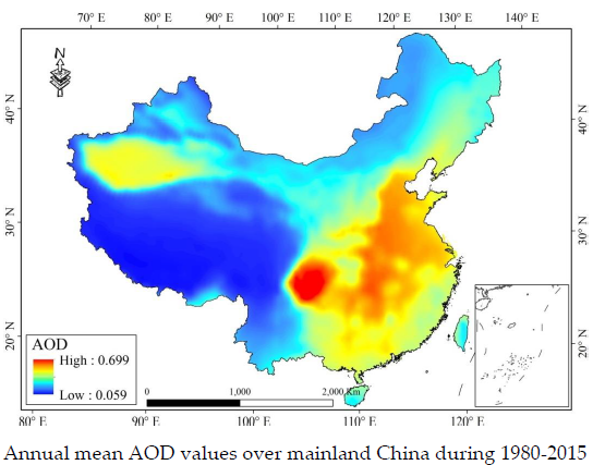
3.4. Spatial and Temporal Variation of AOD-SSR-ARFB in China

3.4.1. Annual Variation of AOD-SSR-ARFB in China

Daily meteorological measurements at 716 CMA stations were used to calculate the daily and monthly mean AOD values over Mainland China using the Genetic_BP model. Then, the daily and monthly mean SSR and ARFB throughout China were calculated using YHM and formula (14). Figure 14 shows the annual mean values of AOD, SSR and ARFB during 1980–2015 over Mainland China. It was obvious that AOD, SSR and ARFB are closely correlated. The R between the annual mean AOD and SSR values was0.715; the R between the annual mean AOD and ARFB values was−0.919; and the R between the annual mean AOD and SSR values was−0.793.

In the beginning of the 1980s, the annual mean AOD values over Mainland China were relatively lower than those in other periods during 1980–2015, due to low anthropogenic aerosol emissions in the beginning of the 1980s. Thus, the ARFB and SSR values in that period were higher than those in other periods. However, the AOD values dramatically fluctuated after 1982, owing to two giant volcano eruptions in 1982 (ALCH Joan volcanic Eruption) and 1992 (Pinatubo Volcanic Eruption). The annual mean AOD value reached the highest ever level (0.321) in 1992 during 1980–2015 over Mainland China. The aerosol radiative effect also reached the strongest level in 1992 (−2.853 MJ m⁻²day⁻¹) during 1980–2015, because of the extremely dense aerosols in the air. Meanwhile, the SSR values degraded in that period owing to the strong aerosol radiative effect. After 1992, the annual mean AOD values gradually decreased. The annual mean AOD values during 1993–2000 were under the level of 0.230. The SSR and ARFB values rose again in that period. In the beginning of 21st century, with the rapid development of economy and population growth in China, the anthropogenic aerosol emissions dramatically rose, thus the AOD values gradually increased in that period. The annual mean AOD values rose from 0.209 (in 2001) to 0.312 (in 2007). The aerosol radiative effect on solar radiation gradually enhanced owing to the rising AOD values. The ranges for the annual mean SSR and ARFB values during 2001–2007 are −2.173 to −2.537 MJ m⁻²day⁻¹ and 15.764 to 15.177 MJ m⁻²day⁻¹, respectively. Since 2008, the anthropogenic aerosol emissions decreased, owing to the formulation and implementation of many environmental protection policies for reducing carbon and aerosol emissions in China. Therefore, the annual mean AOD values in China have gradually decreased since 2008. The ranges of the annual mean AOD, SSR and ARFB values during 2008–2015 were 0.249–0.313, −2.595 to −2.285 MJ m⁻²day⁻¹ and 15.104–16.319 MJ m⁻²day⁻¹, respectively.

3.4.2. Spatial and Temporal Variations of AOD-SSR-ARFB in China

Figure 15 and Figure 16 illustrate the spatial and temporal variations of AOD values over Mainland China. The result show that the AOD values were generally higher in spring than in other seasons, due to the dense aerosol generated by the frequent sandstorms in northern China and the straw combustion in southern China. The monthly mean AOD values from January to December were 0.197, 0.239, 0.299, 0.333, 0.320, 0.287, 0.257, 0.259, 0.237, 0.223, 0.195 and 0.183, respectively. The Sichuan Basin has always been an area with high AOD values, due to the high human activity and the basin topography (hindering aerosol diffusion in the air). The annual mean AOD value during 1980–2015 in the Sichuan Basin was 0.699. The AOD range for the Sichuan Basin from January to December was0.365–0.711. The AOD values in North China Plain and the South Yangtze River were also high, because of intense human activity and favorable humid weather conditions for the formation of haze in the atmosphere; for example the annual mean AOD values in the Huainan and the plain of the middle and lower reaches of the Yangtze River, the North China Plain, the hilly areas of the south of the Yangtze River, the hills and hilly areas in the middle of the Shandong Province were 0.523, 0.513, 0.481, 0.476 and 0.442, respectively. The Tarim and Turpan Basin are also areas with high AOD values, especially in summer owing to frequent dusty weather. The monthly mean AOD values for Tarim and Turpan basin from January to December were 0.179, 0.271, 0.256, 0.187, 0.249, 0.317, 0.407, 0.451, 0.411, 0.334, 0.372 and 0.335, respectively. In contrast, northwestern China has always been an area with low AOD values, due to relatively lower human activity and clear air conditions, for example the ranges for the monthly mean AOD values in Alashan and Hexi Corridor, the western Inner Mongolia high plain, and the eastern Inner Mongolia high plains were 0.151–0.312, 0.149–0.298, and 0.133–0.298, respectively. The Qinghai Tibetan Plateau has always been an area with the lowest annual mean AOD values and monthly mean AOD values, due to the clear atmosphere there, for example, the ranges of the monthly mean AOD values in the Nagqu Plateau and the Ali mountains were 0.0120–0.082 and 0.044–0.106, respectively.

Daily meteorological measurements including surface pressure, surface temperature, relative humidity and sunshine duration at 716 CMA meteorological stations and retrieved AOD values using Genetic_BP model were used to reveal the spatial and temporal variations of SSR over Mainland China. Figure 17 and Figure 18 illustrate these variations. The results show that the monthly mean SSR values gradually increased from January to May and decreased from June to December, owing to the variations of the annual cycle of solar zenith and the maximum sunshine duration in China. The monthly mean SSR for January, February, March, April, May, June, July, August, September, October, November, and December were10.604, 13.349, 17.221, 21.420, 23.998, 24.196, 24.580, 23.250, 19.674, 15.843, 12.207 and 10.218 MJ m⁻²day⁻¹, respectively. The Qinghai Tibetan Plateau has always been an area with the highest SSR values, because of the weaker radiation extinction processes and clear sky conditions; for example, the annual mean SSR for the Zangnan mountain area, the Qiangtang Plateau Lake Basin, the Qaidam Basin and the Southern Qinghai Plateau Gully were22.714, 22.256, 20.175, 20.796 MJ m⁻²day⁻¹, respectively. In contrast, the Sichuan Basin has always been an area with the lowest SSR values, owing to the relatively abundant precipitable water vapor and strong aerosol radiative effect. The annual mean SSR values for Sichuan Basin was 11.721 MJ m⁻²day⁻¹. Northeastern China was also an area with low SSR values, owing to the short sunshine duration in winter and the relatively abundant precipitable water vapor in summer; for example, the annual mean SSR values for Greater Khingan Range was13.624 MJ m⁻²day⁻¹. The SSR values are generally higher in northern China than in southern China in spring and summer, due to the relatively longer sunshine durations and drier air conditions in northern China than that in southern China. However, the SSR values are generally lower in northern China than in southern China in autumn and winter, owing to the relatively shorter sunshine duration in northern China than those in southern China.

Figure 19 and Figure 20 illustrate the spatial and temporal variation of ARFB over Mainland China in different climate zones. The higher the SSR and AOD values are, the lower the ARFB value is. The ARFB are generally stronger in spring and summer than in other seasons, due to the high AOD and SSR values in spring and summer. The monthly mean ARFB values over Mainland China from January to December were−1.353, −1.798, −2.434, −2.978, −2.986, −2.750, −2.636, −2.671, −2.262, −1.890, −1.454 and −1.244 MJ m⁻²day⁻¹, respectively. Eastern China has always been an area with strong ARF, because of the strong human activity intensity and anthropogenic aerosol emissions there; for example, the annual mean ARFB values for North China Plain, the Shandong hilly, the hills in Jiaodong and Liaodong, the Huainan and the middle and lower reaches of the Yangtze River, and the Jiangnan and Nanling Mountains were−3.108, −3.087, −3.006,−2.899 and −2.530 MJ m⁻²day⁻¹, respectively. The Tarim and Turpan Basins are also areas with low ARFB values, owing to the dusty air conditions and high AOD values there. The annual mean ARFB value for Tarim and Turpan Basinswas−2.736 MJ m⁻²day⁻¹. In contrast, the Qinghai Tibet Plateau has always been an area with weak ARF due to the relatively lower AOD values than other climatic zones; for example, the ARFB values for the Alishan Mountain, the Southern Qinghai Plateau Gully, the Qiangtang Plateau Lake Basin and the Zangnan Mountain area were−1.188, −1.115, −1.086 and −0.955 MJ m⁻²day⁻¹, respectively.

4. Conclusions

The applicability of a new AOD retrieval algorithm (Genetic_BP) for estimating daily AOD values over Mainland China was investigated. The estimated AOD values were validated at the CARSNET and AERONET stations. Then, the retrieved AOD values by the Genetic_BP model were used for improving the estimation of SSR and ARFB based on Yang’s hybrid model. The estimated SSR values and ARFB values were evaluated using SSR (CMA) and ARFB (AERONET) measurements. Finally, the spatial and temporal variations of AOD, SSR and ARFB over Mainland China were investigated.

The results show that the Genetic_BP model could be used for estimating AOD values over Mainland China with comparable accuracy. The RMSE, MAE, R and R² for the estimated AOD values at the CARSNET stations were 41.46%, 27.51%, 0.866 and 0.749, respectively. The RMSE, MAE, R and R² for the estimated AOD values at the AERONET stations were 44.98%, 29.23%, 0.865 and 0.747, respectively. The validation results of the estimated SSR and ARFB values also showed good agreement with SSR and ARFB measurements. The RMSE, MAE, R and R² for the estimated SSR values at the CMA stations were 29.27%, 23.77%, 0.948 and 0.899, respectively. The RMSE, MAE, R and R² for the estimated ARFB values at the AERONET stations were −35.47%, −25.33%, 0.843, and 0.711, respectively. Using meteorological measurements from 716 CMA stations, the spatial and temporal variations of AOD, SSR and ARFB values over Mainland China were investigated. The AOD, SSR and ARFB values fluctuated greatly in the beginning of the 1980s over Mainland China, due to two great volcano eruptions: ALCH Joan volcanic Eruption (1982) and Pinatubo Volcanic Eruption (1992). The highest annual mean AOD value (0.321) during 1980–2015 was observed in 1992. Affected by the extremely dense aerosol in the air, the ARF also reached the strongest level in 1992 (−2.853 MJ m⁻²day⁻¹). After 1992, the annual mean AOD values gradually decreased. The annual mean AOD values during 1993–2000 were under 0.230. In the beginning of the21st century, the AOD values gradually increased, because of the increasing anthropogenic aerosol emissions in China in that period. The annual mean AOD values had rose from 0.209 (in 2001) to 0.312 (in 2007). The ARF on SSR also gradually enhanced owing to the rising AOD values. The ranges for the annual mean SSR and ARFB values during 2001–2007 were −2.173 to −2.537 MJ m⁻²day⁻¹ and 15.764–15.177 MJ m⁻²day⁻¹, respectively. Since 2008, many environmental protection policies for reducing carbon and aerosol emissions have been formulated and implemented in China, decreasing anthropogenic aerosol emissions. Thus, the annual mean AOD values in China gradually decreased. The ranges of the annual mean AOD, SSR and ARFB values during 2008–2015 were 0.249–0.313, −2.595 to −2.285 MJ m⁻²day⁻¹ and 15.104–16.319 MJ m⁻²day⁻¹, respectively.

The AOD values were higher in spring than that in other seasons. The largest monthly mean AOD value (0.229) was found in March, while the smallest monthly mean AOD value (0.183) was in December. Relatively larger AOD values were mainly observed in the Sichuan Basin, while smaller AOD values were mainly observed in the Qinghai Tibetan Plateau. The SSR values were generally higher in summer than in other seasons, because of the relatively higher solar zenith and the greater sunshine duration in summer than in other seasons. The SSR values gradually increased from January (6.697 MJ m⁻²day⁻¹) to June (14.028 MJ m⁻²day⁻¹) and decreased from July (13.601 MJ m⁻²day⁻¹) to December (6.140 MJ m⁻²day⁻¹). The Qinghai Tibetan Plateau has always been an area with the highest SSR values, while the Sichuan Basin has always been an area with the lowest SSR values. The ARFB values were closely correlated with AOD and SSR values. The monthly mean ARFB values gradually decreased from January (−1.353 MJ m⁻²day⁻¹) to June (−2.750 MJ m⁻²day⁻¹) and increased from July (−2.636 MJ m⁻²day⁻¹) to December (−1.244 MJ m⁻²day⁻¹), owing the relatively higher AOD values and SSR values in summer than that in other seasons. Eastern China has always been an area with strong aerosol radiative effect, because of the strong human activity and anthropogenic aerosol emissions. The Tarim and Turpan Basin are also areas with strong ARF, owing to the dusty air conditions and high AOD values. In contrast, the Qinghai Tibetan Plateau has always been an area with weak ARF, due to the relatively lower AOD values than in other climate zones.

Certainly, this new approach for improving the estimation of AOD, SSR and ARFB should be further applied and validated in other climatic zones and ecosystems around the world. More attention should be paid to the quantitative correlations among AOD, SSR and ARFB in different climatic zones and ecosystems.

References

1. Iqbal, M. An Introduction to Solar Radiation; Elsevier: New York, NY, USA, 1983. [Google Scholar]
2. Kothe, S.; Dobler, A.; Beck, A.; Ahrens, B. The radiation budget in a regional climate model. Clim. Dyn. 2011, 36, 1023–1036. [Google Scholar] [CrossRef]
3. Shook, K.; Pomeroy, J. Synthesis of incoming shortwave radiation for hydrological simulation. Hydrol. Res. 2011, 42, 433–446. [Google Scholar] [CrossRef]
4. Wang, L.; Gong, W.; Ma, Y.; Zhang, M. Modeling regional vegetation NPP variations and their relationships with climatic parameters in Wuhan, China. Earth Interact. 2013, 17, 1–20. [Google Scholar] [CrossRef]
5. Loutzenhiser, P.G.; Manz, H.; Felsmann, C.; Strachan, P.A.; Frank, T.; Maxwell, G.M. Empirical validation of models to compute solar irradiance on inclined surfaces for building energy simulation. Sol. Energy 2007, 81, 254–267. [Google Scholar] [CrossRef] [Green Version]
6. Bi, J.; Huang, J.; Hu, Z.; Holben, B.N.; Guo, Z. Investigating the aerosol optical and radiative characteristics of heavy haze episodes in Beijing during January of 2013. J. Geophys. Res. Atmos. 2014, 119, 9884–9900. [Google Scholar] [CrossRef] [Green Version]
7. Hauser, A.; Oesch, D.; Foppa, N. Aerosol optical depth over land: Comparing AERONET, AVHRR and MODIS. Geophys. Res. Lett. 2005, 32, 109–127. [Google Scholar] [CrossRef]
8. He, L.; Wang, L.; Lin, A.; Zhang, M.; Bilal, M.; Tao, M. Aerosol optical properties and associated direct radiative forcing over the yangtze river Basin during 2001–2015. Remote Sens. 2017, 9, 746. [Google Scholar] [CrossRef]
9. Torres, O.; Bhartia, P.K.; Herman, J.R.; Sinyuk, A.; Ginoux, P.; Holben, B. A long-term record of aerosol optical depth from TOMS observations and comparison to AERONET measurements. J. Atmos. Sci. 2002, 59, 398–413. [Google Scholar] [CrossRef]
10. Che, Y.; Xue, Y.; Mei, L.; Guang, J.; She, L.; Guo, J.; Hu, Y.; Xu, H.; He, X.; Di, A. Intercomparison of three AATSR Level 2 (L2) AOD products over China. Atmos. Chem. Phys. 2016, 16, 9655–9674. [Google Scholar] [CrossRef]
11. Sayer, A.M.; Hsu, N.C.; Bettenhausen, C.; Jeong, M.J.; Holben, B.N.; Zhang, J. Global and regional evaluation of over-land spectral aerosol optical depth retrievals from SeaWiFS. Atmos. Meas. Tech. 2012, 5, 1761–1778. [Google Scholar] [CrossRef] [Green Version]
12. Hauser, A.; Oesch, D.; Foppa, N.; Wunderle, S. NOAA AVHRR derived aerosol optical depth over land. J. Geophys. Res. Atmos. 2005, 110, D8. [Google Scholar] [CrossRef]
13. Engstrom, A.; Ekman, A. Impact of meteorological factors on the correlation between aerosol optical depth and cloud fraction. Geophys. Res. Lett. 2010, 37, 1480–1493. [Google Scholar] [CrossRef]
14. Martinez-Lozano, J.A.; Utrillas, M.P.; Tena, F. A new inversion algorithm to retrieve instantaneous values for the aerosol optical depth from spectral irradiance measurements. IEEE T. Geosci. Remote. 2000, 38, 579–586. [Google Scholar] [CrossRef]
15. Martinez-Lozano, J.A.; Utrillas, M.P.; Tena, F.; Cachorro, V.E. The parameterisation of the atmospheric aerosol optical depth using the Angstrom power law. Sol. Energy 1998, 63, 303–311. [Google Scholar] [CrossRef]
16. Mulcahy, J.P.; O’Dowd, C.D.; Jennings, S.G.; Ceburnis, D. Significant enhancement of aerosol optical depth in marine air under high wind conditions. Geophys. Res. Lett. 2008, 35, 119–128. [Google Scholar] [CrossRef]
17. Ng, D.; Li, R.M.; Raghavan, S.V.; Liong, S.Y. Investigating the relationship between aerosol optical depth and precipitation over Southeast Asia with relative humidity as an influencing factor. Sci. Rep. UK 2017, 7, 1–13. [Google Scholar] [CrossRef] [PubMed]
18. Sanchez-Romero, A.; Sanchez-Lorenzo, A.; Gonzalez, J.A.; Calbo, J. Reconstruction of long-term aerosol optical depth series with sunshine duration records. Geophys. Res. Lett. 2016, 43, 1296–1305. [Google Scholar] [CrossRef] [Green Version]
19. Wu, J.; Luo, J.G.; Zhang, L.Y.; Xia, L.; Zhao, D.M.; Tang, J.P. Improvement of aerosol optical depth retrieval using visibility data in China during the past 50 years. J. Geophys. Res. Atmos. 2014, 119, 13370–13387. [Google Scholar] [CrossRef]
20. Mei, L.; Xue, Y.; de Leeuw, G.; Holzer-Popp, T.; Guang, J.; Li, Y.; Yang, L.; Xu, H.; Xu, X.; Li, C.; et al. Retrieval of aerosol optical depth over land based on a time series technique using MSG/SEVIRI data. Atmos. Chem. Phys. 2012, 12, 9167–9185. [Google Scholar] [CrossRef] [Green Version]
21. Zhang, H.; Lyapustin, A.; Wang, Y.; Kondragunta, S.; Laszlo, I.; Ciren, P.; Hoff, R.M. A multi-angle aerosol optical depth retrieval algorithm for geostationary satellite data over the United States. Atmos. Chem. Phys. 2011, 11, 11977–11991. [Google Scholar] [CrossRef] [Green Version]
22. Davies, W.H.; North, P.; Grey, W.; Barnsley, M.J. Improvements in aerosol optical depth estimation using multiangle CHRIS/PROBA images. IEEE T. Geosci. Remote. 2010, 48, 18–24. [Google Scholar] [CrossRef]
23. Gao, L.; Li, J.; Chen, L.; Zhang, L.Y.; Heidinger, A.K. Retrieval and validation of atmospheric aerosol optical depth from AVHRR over china. IEEE T. Geosci. Remote. 2016, 54, 6280–6291. [Google Scholar] [CrossRef]
24. Grey, W.; North, P.; Los, S.O.; Mitchell, R.M. Aerosol optical depth and land surface reflectance from Multiangle AATSR measurements: Global validation and intersensor comparisons. IEEE T. Geosci. RemoteSens. 2006, 44, 2184–2197. [Google Scholar] [CrossRef]
25. Li, Y.J.; Xue, Y.; de Leeuw, G.; Li, C.; Yang, L.K.; Hou, T.T.; Marir, F. Retrieval of aerosol optical depth and surface reflectance over land from NOAA AVHRR data. Remote Sens. Environ. 2013, 133, 1–20. [Google Scholar] [CrossRef]
26. Liang, S.L.; Zhong, B.; Fang, H.L. Improved estimation of aerosol optical depth from MODIS imagery over land surfaces. Remote Sens. Environ. 2006, 104, 416–425. [Google Scholar] [CrossRef]
27. Melin, F.; Zibordi, G.; Djavidnia, S. Development and validation of a technique for merging satellite derived aerosol optical depth from SeaWiFS and MODIS. Remote Sens. Environ. 2007, 108, 436–450. [Google Scholar] [CrossRef]
28. Sun, L.; Wei, J.; Bilal, M.; Tian, X.P.; Jia, C.; Guo, Y.M.; Mi, X.T. Aerosol optical depth retrieval over bright areas using landsat 8 OLI images. Remote. Sens. 2016, 8, 23. [Google Scholar] [CrossRef]
29. Zhang, W.H.; Xu, H.; Zheng, F.J. Aerosol optical depth retrieval over east asia using Himawari-8/AHI data. Remote. Sens. 2018, 10, 137. [Google Scholar] [CrossRef]
30. Zhang, Y.; Li, Z.Q.; Qie, L.L.; Hou, W.Z.; Liu, Z.H.; Zhang, Y.; Xie, Y.S.; Chen, X.F.; Xu, H. Retrieval of aerosol optical depth using the empirical orthogonal functions (EOFs) based on PARASOL multi-angle intensity data. Remote. Sens. 2017, 9, 578. [Google Scholar] [CrossRef]
31. Zhong, G.S.; Wang, X.F.; Guo, M.; Tani, H.; Chittenden, A.R.; Yin, S.; Sun, Z.Y.; Matsumura, S. A dark target algorithm for the GOSAT TANSO-CAI sensor in aerosol optical depth retrieval over land. Remote. Sens. 2017, 9, 524. [Google Scholar] [CrossRef]
32. Ali, A.; Amin, S.E.; Ramadan, H.H.; Tolba, M.F. Enhancement of OMI aerosol optical depth data assimilation using artificial neural network. Neural Comput. Appl. 2013, 23, 2267–2279. [Google Scholar] [CrossRef]
33. Radosavljevic, V.; Vucetic, S.; Obradovic, Z. Aerosol optical depth retrieval by neural networks ensemble with adaptive cost function. In Proceedings of the Intenational Conference on Engineering Applications Neural Networks, Thessaloniki, Greece, 29–31 August 2007. [Google Scholar]
34. García Cabrera, R.D.; García Rodríguez, O.E.; Cuevas Agulló, E.; Cachorro, V.E.; Barreto, Á.; Guirado Fuentes, C.; Kouremeti, N.; Bustos, J.J.D.; Romero Campos, P.M.; Frutos, Á.M.D. Aerosol optical depth retrieval at the Izaña Atmospheric Observatory from 1941 to 2013 by using artificial neural networks. Atmos. Meas. Tech. 2015, 9, 9075–9103. [Google Scholar] [CrossRef]
35. Lanzaco, B.L.; Olcese, L.E.; Palancar, G.G.; Toselli, B.M. An improved aerosol optical depth map based on Machine-Learning and MODIS data: Development and application in South America. Aerosol Air Qual. Res. 2017, 17, 1523–1536. [Google Scholar] [CrossRef]
36. Huttunen, J.; Kokkola, H.; Mielonen, T.; Mika, E.J.M.; Lipponen, A.; Reunanen, J.; VilhelmLindfors, A.; Mikkonen, S.; Kari, E.J.L.; Kouremeti, N. Retrieval of aerosol optical depth from surface solar radiation measurements using machine learning algorithms, non-linear regression and a radiative transfer-based look-up table. Atmos. Chem. Phys. 2016, 30, 1–23. [Google Scholar] [CrossRef]
37. Holland, J.H. Genetic algorithms. Sci. Am. 1992, 267, 66–73. [Google Scholar] [CrossRef]
38. Mallet, M.; Roger, J.C.; Despiau, S.; Dubovik, O.; Putaud, J.P. Microphysical and optical properties of aerosol particles in urban zone during ESCOMPTE. Atmos. Res. 2003, 69, 73–97. [Google Scholar] [CrossRef]
39. Chen, Y.C.; Christensen, M.W.; Stephens, G.L.; Seinfeld, J.H. Satellite-based estimate of global aerosol-cloud radiative forcing by marine warm clouds. Nat. Geosci. 2014, 7, 643–646. [Google Scholar] [CrossRef]
40. Kirkevag, A.; Iversen, T. Global direct radiative forcing by process-parameterized aerosol optical properties. J. Geophys. Res. Atmos. 2002, 107, 6–16. [Google Scholar] [CrossRef]
41. Ma, X.; Yu, F.; Luo, G. Aerosol direct radiative forcing based on GEOS-Chem-APM and uncertainties. Atmos. Chem. Phys. 2012, 12, 5563–5581. [Google Scholar] [CrossRef] [Green Version]
42. Myhre, G.; Samset, B.H.; Schulz, M.; Balkanski, Y.; Bauer, S.; Berntsen, T.K.; Bian, H.; Bellouin, N.; Chin, M.; Diehl, T.; et al. Radiative forcing of the direct aerosol effect from AeroCom phase II simulations. Atmos. Chem. Phys. 2013, 13, 1853–1877. [Google Scholar] [CrossRef]
43. Yu, H.; Kaufman, Y.J.; Chin, M.; Feingold, G.; Remer, L.A.; Anderson, T.L.; Balkanski, Y.; Bellouin, N.; Boucher, O.; Christopher, S.; et al. A review of measurement-based assessments of the aerosol direct radiative effect and forcing. Atmos. Chem. Phys. 2006, 6, 613–666. [Google Scholar] [CrossRef] [Green Version]
44. Li, F.; Vogelmann, A.M.; Ramanathan, V. Saharan dust aerosol radiative forcing measured from space. J. Clim. 2004, 17, 2558–2571. [Google Scholar] [CrossRef]
45. Gantt, B.; Xu, J.; Meskhidze, N.; Zhang, Y.; Nenes, A.; Ghan, S.J.; Liu, X.; Easter, R.; Zaveri, R. Global distribution and climate forcing of marine organic aerosol—Part 2: Effects on cloud properties and radiative forcing. Atmos. Chem. Phys. 2012, 12, 6555–6563. [Google Scholar] [CrossRef] [Green Version]
46. Lee, J.; Kim, J.; Lee, Y.G. Simultaneous retrieval of aerosol properties and clear-sky direct radiative effect over the global ocean from MODIS. Atmos. Environ. 2014, 92, 309–317. [Google Scholar] [CrossRef] [Green Version]
47. Ghan, S.; Wang, M.H.; Zhang, S.P.; Ferrachat, S.; Gettelman, A.; Griesfeller, J.; Kipling, Z.; Lohmann, U.; Morrison, H.; Neubauer, D.; et al. Challenges in constraining anthropogenic aerosol effects on cloud radiative forcing using present-day spatiotemporal variability. Proc. Natl. Acad. Sci. USA 2016, 113, 5804–5811. [Google Scholar] [CrossRef] [PubMed]
48. Zhang, H.; Wang, Z.L.; Wang, Z.Z.; Liu, Q.X.; Gong, S.L.; Zhang, X.Y.; Shen, Z.P.; Lu, P.; Wei, X.D.; Che, H.Z.; et al. Simulation of direct radiative forcing of aerosols and their effects on East Asian climate using an interactive AGCM-aerosol coupled system. Clim. Dyn. 2012, 38, 1675–1693. [Google Scholar] [CrossRef]
49. Chang, W.Y.; Liao, H.; Xin, J.Y.; Li, Z.Q.; Li, D.H.; Zhang, X.Y. Uncertainties in anthropogenic aerosol concentrations and direct radiative forcing induced by emission inventories in Eastern China. Atmos. Res. 2015, 166, 129–140. [Google Scholar] [CrossRef]
50. Myhre, G.; Aas, W.; Cherian, R.; Collins, W.; Faluvegi, G.; Flanner, M.; Forster, P.; Hodnebrog, O.; Klimont, Z.; Lund, M.T.; et al. Multi-model simulations of aerosol and ozone radiative forcing due to anthropogenic emission changes during the period 1990–2015. Atmos. Chem. Phys. 2017, 17, 2709–2720. [Google Scholar] [CrossRef]
51. Park, R.S.; Lee, S.; Shin, S.K.; Song, C.H. Contribution of ammonium nitrate to aerosol optical depth and direct radiative forcing by aerosols over East Asia. Atmos. Chem. Phys. 2014, 14, 2185–2201. [Google Scholar] [CrossRef]
52. Marmer, E.; Langmann, B.; Fagerli, H.; Vestreng, V. Direct shortwave radiative forcing of sulfate aerosol over Europe from 1900 to 2000. J. Geophys. Res. Atmos. 2007, 112. [Google Scholar] [CrossRef] [Green Version]
53. Park, R.J.; Kim, M.J.; Jeong, J.I.; Youn, D.; Kim, S. A contribution of brown carbon aerosol to the aerosol light absorption and its radiative forcing in East Asia. Atmos. Environ. 2010, 44, 1414–1421. [Google Scholar] [CrossRef]
54. Leibensperger, E.M.; Mickley, L.J.; Jacob, D.J.; Chen, W.T.; Seinfeld, J.H.; Nenes, A.; Adams, P.J.; Streets, D.G.; Kumar, N.; Rind, D. Climatic effects of 1950–2050 changes in US anthropogenic aerosols—Part 1: Aerosol trends and radiative forcing. Atmos. Chem. Phys. 2012, 12, 3333–3348. [Google Scholar] [CrossRef] [Green Version]
55. Wang, Q.Q.; Jacob, D.J.; Spackman, J.R.; Perring, A.E.; Schwarz, J.P.; Moteki, N.; Marais, E.A.; Ge, C.; Wang, J.; Barrett, S. Global budget and radiative forcing of black carbon aerosol: Constraints from pole-to-pole (HIPPO) observations across the Pacific. J. Geophys. Res. Atmos. 2014, 119, 195–206. [Google Scholar] [CrossRef] [Green Version]
56. Ming, Y.; Ramaswamy, V.; Ginoux, P.A.; Horowitz, L.H. Direct radiative forcing of anthropogenic organic aerosol. J. Geophys. Res. Atmos. 2005, 110. [Google Scholar] [CrossRef] [Green Version]
57. Kim, M.K.; Lau, W.; Kim, K.M.; Lee, W.S. A GCM study of effects of radiative forcing of sulfate aerosol on large scale circulation and rainfall in East Asia during boreal spring. Geophys. Res. Lett. 2007, 34, L24701. [Google Scholar] [CrossRef]
58. Deandreis, C.; Balkanski, Y.; Dufresne, J.L.; Cozic, A. Radiative forcing estimates of sulfate aerosol in coupled climate-chemistry models with emphasis on the role of the temporal variability. Atmos. Chem. Phys. 2012, 12, 5583–5602. [Google Scholar] [CrossRef] [Green Version]
59. Samset, B.H.; Myhre, G. Vertical dependence of black carbon, sulphate and biomass burning aerosol radiative forcing. Geophys. Res. Lett. 2011, 38. [Google Scholar] [CrossRef] [Green Version]
60. Chung, C.E.; Ramanathan, V.; Carmichael, G.; Kulkarni, S.; Tang, Y.; Adhikary, B.; Leung, L.R.; Qian, Y. Anthropogenic aerosol radiative forcing in Asia derived from regional models with atmospheric and aerosol data assimilation. Atmos. Chem. Phys. 2010, 10, 6007–6024. [Google Scholar] [CrossRef] [Green Version]
61. Liu, J.; Scheuer, E.; Dibb, J.; Diskin, G.S.; Ziemba, L.D.; Thornhill, K.L.; Anderson, B.E.; Wisthaler, A.; Mikoviny, T.; Devi, J.J.; et al. Brown carbon aerosol in the North American continental troposphere: Sources, abundance, and radiative forcing. Atmos. Chem. Phys. 2015, 15, 7841–7858. [Google Scholar] [CrossRef]
62. Goto, D.; Nakajima, T.; Takemura, T.; Sudo, K. A study of uncertainties in the sulfate distribution and its radiative forcing associated with sulfur chemistry in a global aerosol model. Atmos. Chem. Phys. 2011, 11, 10889–10910. [Google Scholar] [CrossRef] [Green Version]
63. Fu, S.Z.; Deng, X.; Li, Z.; Xue, H.W. Radiative effect of black carbon aerosol on a squall line case in North China. Atmos. Res. 2017, 197, 407–414. [Google Scholar] [CrossRef]
64. Zhang, Z.Y.; Wu, W.L.; Wei, J.; Song, Y.; Yan, X.T.; Zhu, L.D.; Wang, Q. Aerosol optical depth retrieval from visibility in China during 1973–2014. Atmos. Environ. 2017, 171, 38–48. [Google Scholar] [CrossRef]
65. Xu, X.F.; Qiu, J.H.; Xia, X.G.; Sun, L.; Min, M. Characteristics of atmospheric aerosol optical depth variation in China during 1993–2012. Atmos. Environ. 2015, 119, 82–94. [Google Scholar] [CrossRef]
66. Guo, J.P.; Zhang, X.Y.; Wu, Y.R.; Zhaxi, Y.Z.; Che, H.Z.; La, B.; Wang, W.; Li, X.W. Spatio-temporal variation trends of satellite-based aerosol optical depth in China during 1980–2008. Atmos. Environ. 2011, 45, 6802–6811. [Google Scholar] [CrossRef]
67. Liu, X.Y.; Chen, Q.L.; Che, H.Z.; Zhang, R.J.; Gui, K.; Zhang, H.; Zhao, T.L. Spatial distribution and temporal variation of aerosol optical depth in the Sichuan basin, China, the recent ten years. Atmos. Environ. 2016, 147, 434–445. [Google Scholar] [CrossRef]
68. Li, S.; Wang, T.J.; Xie, M.; Han, Y.; Zhuang, B.L. Observed aerosol optical depth and angstrom exponent in urban area of Nanjing, China. Atmos. Environ. 2015, 123, 350–356. [Google Scholar] [CrossRef]
69. Wang, H.; Yang, L.K.; Deng, A.J.; Du, W.B.; Liu, P.; Sun, X.B. Remote Sensing of aerosol optical depth using an airborne polarimeter over north China. Remote. Sens. 2017, 9, 979. [Google Scholar] [CrossRef]
70. Xie, J.X.; Xia, X.G. Long-term trend in aerosol optical depth from 1980 to 2001 in North China. Particuology 2008, 6, 106–111. [Google Scholar] [CrossRef]
71. Li, S.S.; Chen, L.F.; Tao, J.H.; Han, D.; Wang, Z.T.; Su, L.; Fan, M.; Yu, C. Retrieval of aerosol optical depth over bright targets in the urban areas of North China during winter. Sci. China Earth Sci. 2012, 55, 1545–1553. [Google Scholar] [CrossRef]
72. Sundström, A.M.; Arola, A.; Kolmonen, P.; Xue, Y.; de Leeuw, G.; Kulmala, M. On the use of a satellite remote-sensing-based approach for determining aerosol direct radiative effect over land: A case study over China. Atmos. Chem. Phys. 2015, 15, 505–518. [Google Scholar] [CrossRef]
73. Wendisch, M.; Hellmuth, O.; Ansmann, A.; Heintzenberg, J.; Engelmann, R.; Althausen, D.; Eichler, H.; Müller, D.; Hu, M.; Zhang, Y. Radiative and dynamic effects of absorbing aerosol particles over the Pearl River Delta, China. Atmos. Environ. 2008, 42, 6405–6416. [Google Scholar] [CrossRef]
74. Yang, K.; Koike, T.; Ye, B. Improving estimation of hourly, daily, and monthly solar radiation by importing global data sets. Agric. For. Meteorol. 2006, 137, 43–55. [Google Scholar] [CrossRef]
75. Hecht-Nielsen, R. Theory of the backpropagation neural network. In Neural Networks for Perception; Elsevier: New York, NY, USA, 1992; pp. 65–93. [Google Scholar]
76. Goh, A. Back-propagation neural networks for modeling complex systems. Artif. Intell. Eng. 1995, 9, 143–151. [Google Scholar] [CrossRef]
77. Chi, L.; Lin, L. Application of BP neural network based on genetic algorithms optimization in prediction of postgraduate entrance examination. In Proceedings of the IEEE 3rd International Conference on Information Science and Control Engineering (ICISCE 2016), Bejing, China, 8–10 July 2016; pp. 226–229. [Google Scholar]
78. Yang, K.; Huang, G.W.; Tamai, N. A hybrid model for estimating global solar radiation. Sol. Energy 2001, 70, 13–22. [Google Scholar] [CrossRef]
79. Yang, K.; Koike, T. A general model to estimate hourly and daily solar radiation for hydrological studies. Water Resour. Res. 2005, 41. [Google Scholar] [CrossRef] [Green Version]
80. Gueymard, C.A. Direct solar transmittance and irradiance predictions with broadband models. Part I: Detailed theoretical performance assessment. Sol. Energy 2003, 74, 355–379. [Google Scholar] [CrossRef]
81. Gueymard, C.A. Direct solar transmittance and irradiance predictions with broadband models. Part II: Validation with high-quality measurements. Sol. Energy 2003, 74, 381–395. [Google Scholar] [CrossRef]
82. Xia, X. A critical assessment of direct radiative effects of different aerosol types on surface global radiation and its components. J. Quant. Spectrosc. Radiat. Transf. 2014, 149, 72–80. [Google Scholar] [CrossRef]
83. Qin, W.; Wang, L.; Lin, A.; Zhang, M.; Xia, X.; Hu, B.; Niu, Z. Comparison of deterministic and data-driven models for solar radiation estimation in China. Renew. Sustain. Energy Rev. 2018, 81, 579–594. [Google Scholar] [CrossRef]
84. Qin, J.; Tang, W.; Yang, K.; Lu, N.; Niu, X.; Liang, S. An efficient physically based parameterization to derive surface solar irradiance based on satellite atmospheric products. J. Geophys. Res. Atmos. 2015, 120, 4975–4988. [Google Scholar] [CrossRef] [Green Version]
85. Leckner, B. The spectral distribution of solar radiation at the earth’s surface—Elements of a model. Sol. Energy 1978, 20, 143–150. [Google Scholar] [CrossRef]
86. Ångström, A. Techniques of determinig the turbidity of the atmosphere. Tellus 1961, 13, 214–223. [Google Scholar] [CrossRef]
87. Xu, X.; Du, H.; Zhou, G.; Mao, F.; Li, P.; Fan, W.; Zhu, D. A method for daily global solar radiation estimation from two instantaneous values using MODIS atmospheric products. Energy 2016, 111, 117–125. [Google Scholar] [CrossRef]
Figure 1. Spatial distribution of the CARSNET, AERONET, SSR and CMA stations used in this study.
Remotesensing 10 01022 g001
Figure 2. Monthly variations of metrological parameters for CARSNET, AERONET, SSR and CMA stations: (a) T; (b) P; (c) RH; and (d) SH.
Remotesensing 10 01022 g002
Figure 3. The topographic zones over Mainland China.
Remotesensing 10 01022 g003
Figure 4. The basic schematic architecture of the BP neural network used in this study.
Remotesensing 10 01022 g004
Figure 5. General structures of the Genetic_BP model.
Remotesensing 10 01022 g005
Figure 6. Validations of the estimated AOD by the Genetic_BP at the CARSNET and AERONET stations during 2002–2014 (a for CARSNET stations, b for AERONET stations).
Remotesensing 10 01022 g006
Figure 7. Monthly variation of the statistical indicators representing the model accuracy for the estimated AOD values at the CARSNET and AERONET stations: (a,b) CARSNET stations; and (c,d) AERONET stations)during 2002–2014.
Remotesensing 10 01022 g007
Figure 8. Validation of AOD products from MODIS and MERRA2during 2002–2014: (a) MODIS08DB; (b) MODIS08DTBC; (c) MODIS08MEAN; (d) MODIS04DB; (e) MODIS04DT; and (f) MERRA2.
Remotesensing 10 01022 g008
Figure 9. Validation of the estimated SSR values by the YHM algorithm at 96 CMA radiation stations during 2002–2014.
Remotesensing 10 01022 g009
Figure 10. Spatial distribution of the RMSE and MAE of YHM over Mainland China (a for RMSE, b for MAE).
Remotesensing 10 01022 g010
Figure 11. Monthly variation of the statistical indicators representing the accuracy of the YHM algorithm at the CMA radiation stations during 2002–2014 (a for CARSNET stations, b for AERONET stations).
Remotesensing 10 01022 g011
Figure 12. Validation of estimated ARFB at AERONET stations during 2002–2014.
Remotesensing 10 01022 g012
Figure 13. Monthly variations of the statistical indicators representing the model accuracy for the estimated ARFB values at AERONET stations during 2002–2014 (a for CARSNET stations, b for AERONET stations).
Remotesensing 10 01022 g013
Figure 14. Annual mean values of AOD, SSR and ARFB values during 1980–2015 over Mainland China.
Remotesensing 10 01022 g014
Figure 15. Distribution of the annual mean AOD values over Mainland China during 1980–2015.
Remotesensing 10 01022 g015
Figure 16. Distribution of the monthly mean AOD values throughout China during 1980–2015: (a) January; (b) February; (c) March; (d) April; (e) May; (f) June; (g) July; (h) August; (i) September; (j) October; (k) November; and (l) December.
Remotesensing 10 01022 g016
Figure 17. Distribution of the annual mean SSR values over Mainland China during 1980–2015.
Remotesensing 10 01022 g017
Figure 18. Distribution of the monthly mean SSR values throughout China during 1980–2015: (a) January; (b) February; (c) March; (d) April; (e) May; (f) June; (g) July; (h) August; (i) September; (j) October; (k) November; and (l) December.
Remotesensing 10 01022 g018
Figure 19. Distribution of the annual mean ARFB values over Mainland China during 1980–2015.
Remotesensing 10 01022 g019
Figure 20. Distribution of the monthly mean ARFB values throughout China during 1980–2015: (a) January; (b) February; (c) March; (d) April; (e) May; (f) June; (g) July; (h) August; (i) September; (j) October; (k) November; and (l) December.
Remotesensing 10 01022 g020