Abstract
Quantitative Precipitation Estimates (QPEs) obtained from remote sensing or ground-based radars could complement or even be an alternative to rain gauge readings. However, to be used in operational applications, a validation process has to be carried out, usually by comparing their estimates with those of a rain gauges network. In this paper, the accuracy of three QPEs are evaluated for three extreme precipitation events in the last decade in the southeast of the Iberian Peninsula. The first QPE is PERSIANN-CCS (Precipitation Estimation from Remotely Sensed Information using Artificial Neural Networks - Cloud Classification System) , a satellite-based QPE. The second and the third are QPEs from a meteorological radar with Doppler capabilities that works in the C band. Pixel-to-point comparisons are made between the values offered by the QPEs and those obtained by two networks of rain gauges. The results obtained indicate that all the QPEs were well below the rain gauge values in extreme rainfall time slots. There seems to be a weak linear association between the value of the discrepancies and the precipitation value of the QPEs. The main conclusion, assuming the information from the rain gauges as ground truth, is that neither PERSIANN-CCS nor radar, without empirical calibration, are acceptable QPEs for the real-time monitoring of meteorological extremes in the southeast of the Iberian Peninsula.
1. Introduction
Precipitation is a highly relevant feature in Earth sciences. Precipitation estimations with good spatial and temporal resolution are important in hydrology, climate research [1], ecology and meteorology. Precipitation estimations might be the most important meteorological input for calibrating and using hydrological and ecological models [2].
Meteorological radars have been used for flood warnings, but they are very expensive to set up and maintain, and their coverage is limited in mountainous areas [3]. In fact, the first operational network of meteorological radars in tropical mountain areas has only been operational for a few years [4]. These authors and Nikolopoulos et al., 2013 [5] also identified the difficulty of maintaining radar networks in developing countries. This lack of adequate data for precipitation monitoring limits the scope for hydro-meteorological research and the use of physical or statistical models for water resources management [6].
Rain gauge networks have been used as primary source of rainfall measurements for over a century. However, while these devices provide direct and accurate (relative to other sensors) rainfall measurements, they are associated with small sampling areas [5]. Another problem arises when using rain gauges as a source of information of precipitation: rain gauges perform point specific measurements and, even in very dense networks, it may not be possible to capture the spatial variability of precipitation, especially when working at subhour scales [7] or when dealing with very localised convective or orographic precipitation.
The Quantitative Precipitation Estimates (QPEs) obtained by remote sensing can complement or be considered an alternative to rain gauge measurements. Satellite-based QPE are valuable continuous records on several temporal [8] and spatial scales and can provide acceptable good estimations of precipitation in “un-gauged” regions, such as oceans, hard-to-reach mountainous areas or deserts [2]. We agree with Zambrano-Bigiarini et al. (2017) [9] that satellite-based QPEs provide an unprecedented opportunity for a wide variety of meteorological and hydrological applications.
In recent decades, the frequency of flood disasters in European Union (EU) has increased [10]. In Spain, floods are the natural hazard with the greatest territorial impact and are responsible for great socio-economic losses [11]. Spain is also the EU country most affected by flash floods [10]. In the southeast of the Iberian Peninsula these phenomena have caused a very high number of deaths and millions of economic losses. Recent examples are the three events analysed in Section 2.2.
It is not possible for all small and medium sized basins that may produce a flooding event to measure runoff in the channels, so precipitation intensity remains the most used source of information during extreme weather events. Therefore, regardless of the methodology or type of modelling used, warning accuracy will depend on the accuracy of the precipitation estimation [5].
Serrano Notivoli et al. (2017) [12] developed a high resolution daily precipitation grid for the whole of Spain from rain gauge data. They also analysed the estimation uncertainties, concluding that the highest uncertainty values appear in SE Spain, the study area of this paper. The reason is that most of the precipitation in this area is produced by convective systems generated over the Mediterranean Sea interacting with Potential Vorticity Streamers (PVS) or cut-offs in the higher troposphere [13]. In such conditions, the entrance of wet air masses to the land is driven by the relief pattern and the wind direction. The interaction of both factors produces highly localised upwinds and a very irregular precipitation pattern that are very difficult to estimate by interpolation with daily rain gauge data alone. This is obviously a considerable handicap for hydrological forecasting. This concentration and variability justifies any attempt to obtain better rainfall estimations using remote sensing products.
Satellite-based QPEs have not been well integrated into operational and decision-making applications because of the lack of rigorous validation and uncertainty analysis [14]. Hong et al. (2007) [15] pointed out that the strong spatio-temporal variability of precipitation makes it necessary to rigorously assess QPE accuracy before the estimates can be used with confidence. In a recent paper, Zambrano-Bigiarini et al. (2017) [9] claimed that no satellite-based QPE can be generally considered more accurate than any others on a daily scale, and that accuracy must be assessed on a case-by-case basis in the study area in question.
Accuracy estimations of global products such as PERSIANN-CCS (Precipitation Estimation from Remotely Sensed Information using Artificial Neural Networks-Cloud Classification System) in areas where rain gauge data is available might be useful to estimate if they are accurate enough to be used in areas where rigurous validation is impossible due to the absence of rain gauge information with which to compare satellite-based QPEs.
The aim of this research was to evaluate the accuracy of two kinds of QPEs during heavy rainfall events. The intention was also to ascertain whether any of the QPEs could be regarded as a good substitute for the information provided by a rain gauge network if it malfunctions.
We have compared precipitation measurements of two rain gauge networks with those estimated by a satellite-based QPE (PERSIANN-CCS) and two ground-based QPEs (meteorological radar) during the three most important heavy rainfall episodes recorded during the last ten years in the southeast of the Iberian Peninsula (Spain). Comparisons are made with aggregated data, using statistics for the entire study area and for the most affected river basins, on the one hand, and in a disaggregated manner, doing the same for the rain gauge that recorded the greatest accumulations and intensities of precipitation, on the other. The comparisons are made on a spatial basis, using interpolation to map the differences in accumulated precipitation between the three QPEs and the rain gauges on the one hand, and between the QPEs, on the other. Comparisons are also made with a temporal perspective using statistics on the agreement among precipitation sources calculated on an hourly scale.
2. Materials and Methods
2.1. Study Area
The research was carried out in the terrestrial portion of the Segura River Basin District, located in south-eastern Spain (Figure 1), with a surface area of 18,740 km covering the Segura River basin and other small coastal basins [16]. It is a territory with scarce and irregular rainfall, high temperatures and a high annual number of hours of sun. There is a NW-SE precipitation gradient that ranges from approximately 1000 mm/year in the headwaters of the Segura river to less than 300 mm/year in the coastal zone [17]. With the exception of the Segura river, the most common channels are ramblas (ephemeral rivers), frequently responsible for flash floods [11]. Although it is a small river basin district, its management is quite complex as a result of having water resources from different sources (surface and groundwater resources, desalination, transfers and reuse) and multiple uses that compete for the scarce water resources [18].
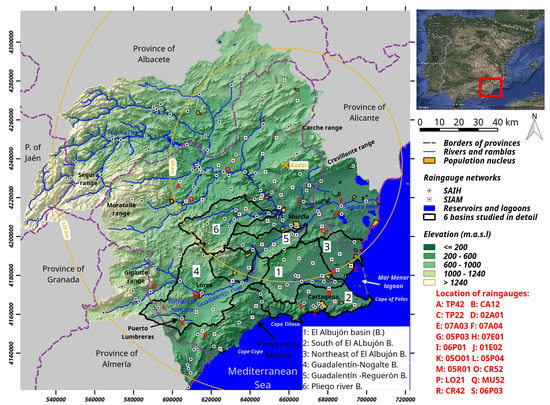
Figure 1.
Map of the study area, the Segura River Basin District. Coordinate Reference System is ETRS89 with projected coordinates (EPSG—European Petroleum Survey Group—code: 25830).
2.2. Rainfall Events
Three very intense precipitation events, in the last decade were identified and characterized. All off them were convective in nature. The first one took place on 27–28 September 2009 and affected the Campo of Cartagena area. The rain gauge 06P03, located about 5 km NW of La Vaguada, recorded 199 mm in 29 h and the CA12 rain gauge, located in La Palma, recorded 268 mm in 30 h. The two mentioned rain gauges were located in the municipality of Cartagena, and the rainfall produced several flash floods in the Campo de Cartagena basins (basins number 1, 2 and 3 in Figure 1).
The second event occurred during the first half of 28 September, 2012. The rain gauge 05P03, located in the foothills of Sierra del Gigante (Municipality of Lorca), recorded 124 mm in five hours and the 05O01 rain gauge, located in Puerto Lumbreras, recorded 153 mm in six hours. Massive flash floods were registered in the Nogalte (Figure 2) and Guadalentín basins (basin number 4 in Figure 1).
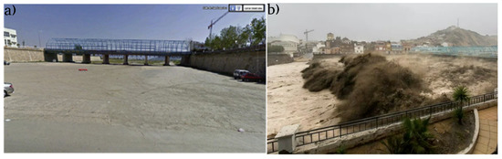
Figure 2.
The rambla of Nogalte is normally dry (a) and only runs water when there is heavy rainfall in the upper basin as on the 28 September 2012 event (b). Sources: (a) [19]; (b) CHS (Segura Basin Hydrological Confederation) , 2013.
The most recent event was registered between 17 and 19 December 2016, and was the most important meteorological episode of the whole year for the Iberian Peninsula. The highest rainfall intensities were registered in Campo of Cartagena and the east coast of the study area, where the rainfall exceeded 50 mm in one hour in the Torre Pacheco (TP42) and San Javier (TP22) rain gauges. Areas close to the Mar Menor lagoon, which environment has undergone a strong process of global transformation due to tourist [20] and farming activity, were severely affected by the storm and the consequent flooding.
The three analyzed events present a high return period. The event of September 2009 corresponds to 200-years return period. Moreover, both events of September 2012 and December 2016 correspond to 500-years return period. The estimations were based on Ministerio de Fomento (1999) [21] by applying the SQRT-ETmax cumulative distribution function.
2.3. Satellite-Based Quantitative Precipitation Estimates : PERSIANN-CCS
PERSIANN-CCS [1] is a system based on satellite imagery and pattern recognition techniques applied for the automatic classification of several types of clouds in order to estimate the rainfall in each pixel.
PERSIANN-CCS produces QPEs with a time resolution of one hour, a spatial resolution of 0.04 (≈ in Spanish latitudes), with near to global coverage (between 60N and 60S) and a lag time of approximately one hour (near-real time). PERSIANN-CCS is a product purely derived from satellite observations, i.e., it is not calibrated using ground observations [22]. Since PERSIANN-CCS is available in near-real time, it is suitable for use in flood warning and management applications [3,23], especially in large river systems such as the Segura or Guadalentín river basins where the one-hour temporal resolution has little impact on hydrological analysis compared to smaller flash floods prone basins [24]. Very promising advances have been made in the calibration of PERSIANN-CCS with data from other satellite data [25], but, unfortunately, these products are not available in near-real time.
2.4. Ground-Based Quantitative Precipitation Estimates : Meteorological Radar
Radar data from the Spanish Meteorology Service (AEMET) has been used. This apparatus operates in the C band (5.6 GHz) and is equipped with Doppler capability. It currently provides data for a circle of 240 km radius (long range mode) and provides images in Cartesian local projection according to Lambert’s conformal conical centered on the radar (38.27N, 1.19W). Each image consists of 480 × 480 pixels and a spatial resolution of when operating in long-range mode. When working in short-range mode, it provides information for a circle area of 120 km radius and a spatial resolution of . Hourly accumulated precipitation data, the QPE with highest temporal resolution offered by AEMET, were used in this work. Meteorological radar data is not freely accessible. An official request to AEMET is required and the price is 0.51 euros/image plus taxes, except when a discount for scientific research is approved by AEMET.
Although operational QPEs provided by AEMET are used in this research, we will briefly describe how the radar reflectivity is transformed to rainfall intensity. The reflectivity images have a temporal resolution of 10 min and store the reflectivity Z in dB (), this is transformed to reflectivity (Z) in using the equation , after that the rainfall intensity in is obtained applying Marshall-Palmer’s Z-R ratio [26] (p. 178) . The QPE CAPPI (constant altitude plan position indicator) with a temporal resolution of 1 hour is obtained after averaging the 6 corresponding intensities.
For the 2009 episode, hourly accumulation data, based on CAPPI , are available for working in short range mode. No meteorological radar data are available for the 2012 episode due to a power failure because of the storm . Finally, for the 2016 episode, an hourly QPE called SRI (surface rainfall intensity) was used. This is an improved product that takes into account the nature of the precipitation (convective or stratiform) before applying, or not, a correction for the vertical reflectivity profile. The main advantage of radar QPEs over a satellite-based QPEs is a lag time of about 7 min from the end of the accumulation period, as shown in the image metadata.
2.5. Rain Gauges
PERSIANN-CCS and radar data were compared with two rain gauge networks. The SIAM (Agroclimatic Information Service of Murcia) network consists of several automatic rain gauges (45 in the 2009 event, 44 in the 2012 event and 47 in the 2016 event) with a temporal resolution of one hour. The second network is the SAIH-Segura (Automatic Hydrological Information System of the Segura River Basin) operated by the Water Authority (Segura Basin Hydrological Confederation, CHS). It had 64 rain gauges operative for the 2009 event, 66 for the 2012 event, and 106 for the 2016 event. The time resolution of this network is 5 min. The CRS of the two rain gauge networks is ETRS89/UTM zone 30N (EPSG code: 25830). Both networks were joined to obtain a more dense network. In 2009 and 2012 there was a rain gauge for every 173 km, for the 2016 event the density increased to a rain gauge every 124.5 km.
The data from SIAM network are evaluated and validated internally before being made available to the public. SAIH-Segura network data for the 2009 and 2012 events are reported in the system as “filtered and consolidated”. Only for the 2016 event did the data appear at the time of the download as “provisional, obtained in real time without checking”. Regardless of this, the precipitation data have been analyzed to eliminate possible erroneous values prior to comparison with the QPEs using the methodology proposed by Velasco-Forero et al. (2009) [27], which is: Rain gauges with cumulative precipitation lower than 1.5 mm from the entire event were discarded from the analysis when the cumulative radar precipitation was more than 10 mm. In addition, long periods of inactivity of the rain gauges have been monitored to ensure that they correspond to the same pattern in the radar data. After the corresponding analyses, one rain gauge was removed from the SIAM network in the 2009 event and another one from the SAIH-Segura network in the 2016 event.
2.6. Assesssment of Quantitative Precipitation Estimates
As proposed by other authors [9,28,29,30] a point-to-pixel analysis was used to compare rain gauge data with the QPEs. The rain gauge layers were reprojected to the CRS of the QPE to avoid uncertainties associated with the resampling of the pixels, and when more than one rain gauge intersected with a QPE pixel, the mean value of the rain gauges was used for the comparison. When this is the case, the number of pixels available for comparison (second column of the Table 1) is not the same as the number of rain gauges.

Table 1.
Statistics of agreement and linear association between rain gauges and the corresponding pixels of PERSIANN-CCS and radar (additive component of the differences), for the three events in the basins most affected by each event.
To implement a point-to-pixel comparison is a difficult task because of several uncertainties to be taken into account when evaluating the statistics derived from the comparison. For example, the spatial support of QPE and rain gauges is different. The rain gauge entrance (in all cases less than 0.05 m) can be approximated to a point measurement, while the values stored in the pixels of the QPEs correspond to averages over the volume of a grid cell [7]. This causes a smoothing of the QPEs’ values compared to the punctual measurements of the rain gauges [31]. Therefore, the differences in the values of rain gauges and QPE pixels are not only due to errors in the QPEs, but also to differences in spatial support [7]. This problem increases if the spatial resolution of the QPE is smaller, so the problem is much more serious for PERSIANN-CCS than for both radar images.
In addition, the finescale variability of precipitation even at short distances, especially with convective precipitation, which cannot be represented by a dispersed network of rain gauges [15], introduces uncertainty into the precipitation values averaged over large areas.
Such problems require careful interpretation of the observed differences when a point-to-pixel comparison is applied. According to Schiemann et al. (2011) [7], accepting the assumption that the above effects lead to a random component in the pluviometer-QPE differences, comparisons made for a large number of rain gauges (such as that used in this research) can provide some guidance concerning the accuracy obtained by different QPEs. For these reasons, the word “error” is avoided as the word “difference” is considered more appropriate; although terms such as overestimate or underestimate (always using the rain gauge value as the baseline) are introduced with the intention of simplifying the text as much as possible.
The statistics calculated to report the additive component of the differences between rain gauges and QPEs were: , where was the measured precipitation for a given rain gauge during a given time interval and was the estimated precipitation for the QPE at the pixel intersecting with the location of the previous rain gauge for the same time interval; the average rainfall of rain gauges as ; the average precipitation of the QPE, ; the root mean square difference as ; the mean absolute difference as ; the bias as ; Pearson’s linear correlation coefficient [32] (p. 134); the relative MAD as and the relative RMSD as .
In very intense but very localised precipitations, the use of these statistics might produce misleading results since the values close to zero have a downward influence on the value of the statistic. In research such as this, the use of conditional statistics is desirable. In our case the condition was that either the rain measure () or the QPE estimate () was equal to or greater than 1 mm/h. Conditional statistics are represented in this work with an asterisk in front of the statistic’s name, so the conditional MAD is *MAD.
In addition to the aforementioned statistics, others, related to the multiplicative component of the differences, were calculated. This is the main component in many of the errors present in meteorological radar QPEs [33]. These statistics are usually calculated only with the cases in which both sources register precipitation. A 0.2 mm/h threshold, the lowest resolution of all the sensors used (some SIAM network rain gauges), was used. For each episode the bias in dB was calculated as [34]. This statistic expresses the overall agreement between QPEs estimates and ground truth given that both instruments register precipitation [35]. The scatter was also calculated as where refers to the 16% percentiles of the distribution. The scatter refers to the spread of hourly QPE-gauge ratios when pooling all rain hours and gauges together [36]. Considering that this statistic is not very sensitive to outliers, it should be interpreted with caution when studying precipitation associated with high return period events.
Different comparisons were carried out to determine the degree of agreement between the three sources of information. A comparison of the precipitation values at a given location was made (Figure 9 and Figure 10). A comparison of statistics has also been made for the course of the three storms in different spatial areas (Figure 3, Figure 4 and Figure 5). This allowed us to identify the QPE whose rainfall values were closest to those of the rain gauges and to relate the observed differences with the precipitation intensities measured by the rain gauges. An analysis of the spatial distribution of the total accumulation of events has been carried out to compare the QPEs and identify, for each of them, the places where the greatest differences with respect to rain gauges occurred. Interpolation techniques were used for this purpose. Finally, a pixel-by-pixel comparison, as proposed by Nguyen et al. (2015) [24], between the radar and PERSIANN-CCS was carried out by generating a mapping of statistics and linear association between the QPEs for the 2009 and 2016 events (Figure 8).
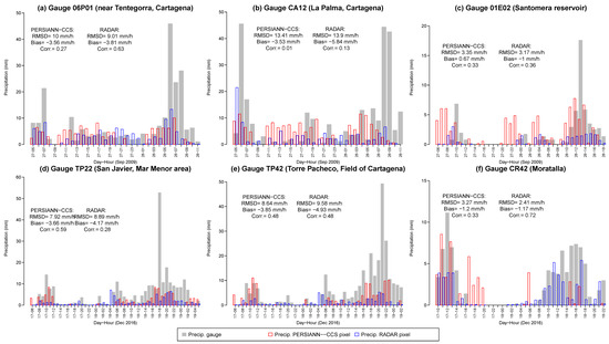
Figure 9.
Hyetographs and associated statistics of PERSIANN-CCS, radar and the corresponding rain gauges of SIAM or SAIH-Segura. (a–c), 2009 event. (d–f), 2016 event.
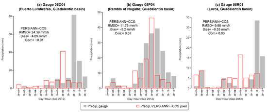
Figure 10.
Hyetographs and associated statistics of PERSIANN-CCS and the corresponding rain gauges of SAIH-Segura.
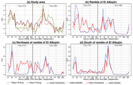
Figure 3.
Temporal variation of Mean Absolute Differences (MAD) and rain gauge mean precipitation (Mean Precip.) in different spatial areas of the study area (PERSIANN-CCS and radar) during the 2009 event.
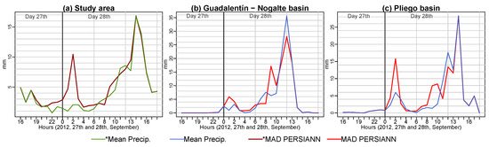
Figure 4.
Temporal variation of Mean Absolute Differences (MAD) and rain gauge mean precipitation (Mean Precip.) in different spatial areas of the study area (PERSIANN-CCS) during the 2012 event.
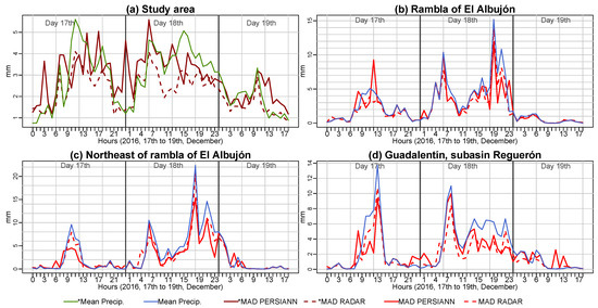
Figure 5.
Temporal variation of Mean Absolute Differences (MAD) and rain gauge mean precipitation (Mean Precip.) in different spatial areas of the study area (PERSIANN-CCs and radar) during the 2016 event.
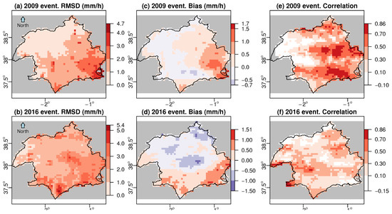
Figure 8.
Comparision statistics between PERSIANN-CCS and radar hourly precipitation. WGS84 projection (EPSG code 4326). Maps (a,c,e) from 0500 UTC 27 September to 0100 UTC 30 September 2009. Maps (b,d,f) from 0000 UTC 17 December to 1900 UTC 19 December 2016.
3. Results
3.1. Statistics
Table 1 shows the statistics of the degree of agreement and linear association among rain gauges and QPEs. The number of pixels for comparison may not be equal for the same event in the two QPEs analysed due to their different spatial resolutions. The observations column indicates the number of pairs of precipitation values taken into account to calculate the statistics. In all the events, the number of non-conditional observations in the study area more than doubles the conditional observations. These large differences in extreme precipitation events reflect their highly localised character. Focusing on the basin with the greatest accumulation of precipitation in the 2009 event (647 km), the number of conditional observations is approximately 72 percent less than the number of non-conditional observations. In the 2012 event, the percentage of conditional observations is less than 50 in the sub-basin with the greatest accumulation of precipitation.
In the September 2009 event (Table 1a), the RMSD of the entire study area is moderate, 3.5 mm/h for PERSIANN-CCS and 2.9 mm/h for radar. However, this value is partly due to the high number of hours in which both PERSIANN-CCS and radar have precipitation values below 1. The conditional RMSD values increase to 5.2 and 4.9 mm/h, respectively. The relative values of RMSD indicate that the statistic is 1.8 times the mean precipitation value of PERSIANN-CCS and 1.4 times that of radar. Both PERSIANN-CCS and radar show worse agreements with the rain gauges located in the basins most affected by the storm. For the whole study area, the *bias values of PERSIANN-CCS indicate that the underestimated values compensate for the overestimated values. Both bias and *bias values are larger with radar for the whole study area and sub-basins. Correlation values, on the other hand, both conditional and non-conditional, are larger with radar in all cases.
No radar data were available for the 2012 event (Table 1b). PERSIANN-CCS statistics shows some degree of agreement with those of the 2009 event. The *RMSD is larger and this increase is proportional to the variation in precipitation intensity, which in the 2012 event was greater. *rRMSD and *rMAD values remain constant. In the 2012 event bias and *bias values indicate that PERSIANN-CCS as a whole underestimates precipitation and the correlation values indicate that the linear association is not strong.
For the 2016 event (Table 1c) another QPE from the same radar (SRI) was used. In a first analysis the values of *RMSD are similar to those of the 2009 episode. Significant changes in statistics can be seen when moving from conditional to non-conditional statistics. In the two QPEs, precipitation tends to be underestimated, the values for the whole basin being similar in both; however, if the most affected basins are taken into account, in two of them (Rambla of El Albujón basin -Al.- and Basin located at Northeast of rambla of El Albujón -NE. Al-) the *bias is unfavourable to radar and in the third the values are the same (Subasin of Guadalentín river where the Reguerón channel is located -G. Re.-). With respect to the correlation of the whole area, radar shows values that are closer to those of the rain gauges, but if the three basins analyzed are considered, the situation is variable. For this episode and according to the data provided by this table and from the point of view of the additive component of the differences, it cannot be said that either QPE gives results that are more similar to the rain gauge results measurements.
With respect to the multiplicative components of the differences (Table 2) bias of PERSIANN-CCS is close to 0 especially in the 2009 event, whereas in the two events in which radar is available is much lower than in this one. The values of radar bias are quite high. The scatter values inform us that in the QPEs, and for all events, there is a very high dispersion, in both cases higher in PERSIANN-CCS and with the highest value in the 2012 event.
Table 2.
Statistics of the multiplicative component of the differences between rain gauges and the corresponding pixels of PERSIANN-CCS and radar. Obs. stands for number of observations.
3.2. Hourly Monitoring of Differences
The analysis of the temporal evolution of the intensities and of the agreement measures between the two estimates give an indication of the virulence of the storm as well as the possible hydrological response of the basin. This analysis is also important to validate precipitation products as it allows us to assess whether the analyzed QPE, in the absence of other sources of information, correctly estimates the evolution of the storm or the quantities precipitated in small basins prone to flash floods.
Figure 3a shows the evolution of the mean conditional precipitation according to rain gauges and the conditional MAD for the whole study area. Figure 3b–d shows the same no-conditional statistics.
In the study area, both PERSIANN-CCS and radar *MAD values are very similar to when this value is high (Figure 3a). The *MAD of radar tends to be low when the is low, while this is not the case with PERSIANN-CCS. If we focus on the rain gauges of the Albujón basin we see that the MAD is proportional to the intensity of the precipitation and the peaks of MAD in both PERSIANN-CCS and radar coincide with the two peaks of . For the other two basins the results are similar. Both PERSIANN-CCS and radar have very high MAD for the magnitude of .
Figure 4 shows the results for the 2012 event. MADs coincides with average precipitation at peak precipitation levels and again there is overestimation when average precipitation is low.
The results of the 2016 event are shown in Figure 5. In the study area, the temporal evolution of the *MAD indicates that this statistic, as in previous events, is closely related to the precipitation recorded by the rain gauges, although PERSIANN-CCS overestimates precipitation when it was low. The *MADs of PERSIANN-CCS shows very erratic estimations, with strong ups and downs in very short periods of time. In this sense, radar *MADs are much more constant and correlated for both high and low mean precipitation values. Radar patterns are more accurate than those of PERSIANN-CCS. The results for the three basins most affected by the storm (Figure 5b–d) point to a much more similar behaviour between the two QPEs. Again, average precipitation peaks reflect peaks in MAD in the two QPEs, although the MAD values of PERSIANN-CCS are usually higher.
3.3. Side-By-Side Comparison of Accumulated Precipitation
To correctly validate QPEs, the map of precipitation accumulations of the whole event (Figure 6) was compared with the map of the differences observed (Figure 7) for the QPEs and the three events analyzed. Each map was generated with the native resolution of the QPE, which is evident from the appearance of the maps, especially in the case of the 2009 event, when the radar worked in short-range mode. To interpolate the rain gauge results (Figure 6c,f,i and Figure 7) we used Ordinary kriging with automatic fitting procedures using the R geostatistical library gstat [37].
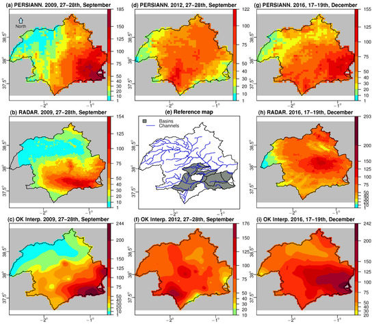
Figure 6.
Total precipitation accumulations of the three events in mm. WGS projection (EPSG code 4326). Maps (c,f,i) are the result of an Ordinary kriging interpolation. Maps (a–c) from 0500 UTC 27 September to 0100 UTC 30 September 2009. Maps (d,f) from 1600 UTC 27 September to 1900 UTC 28 September 2012. (g–i) from 0000 UTC 17 December to 1900 UTC 19 December 2016.
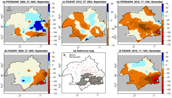
Figure 7.
Interpolation by Ordinary kriging of the total accumulation differences (QPE pixel minus rain gauge) in each event in mm. WGS84 projection (EPSG code 4326). Maps (a,b) from 0500 UTC 27 September to 0100 UTC 30 September 2009. Maps (c) from 1600 UTC 27 September to 1900 UTC 28 September 2012. Maps (e,f) from 0000 UTC 17 December to 1900 UTC 19 December 2016.
The 2009 event shows an east-west rainfall gradient according to PERSIANN-CCS, with the highest values in the east. The maximum value of this QPE is 184 mm and the average value is 50 mm. The radar estimate for the 2009 episode, on the other hand, seems to be distributed in horizontal bands, with the highest values concentrated at the latitude of the coastline of the Region of Murcia descending towards the north and towards the south. The maximum radar accumulation value in this episode is 154 mm and the average is 30.7 mm, both much lower than the values provided by PERSIANN-CCS. With regard to the interpolation of differences (Figure 7a,b). The mean of the absolute values of the map is 17.7 mm, while the same statistic on the radar map is 19.4 mm. With respect to the maximums, the PERSIANN-CCS is 104.5 mm and the radar is 169.2 mm. The map of interpolated radar differences (Figure 7b) shows very strong underestimations near Cartagena and the mouth of the Segura river, while these values tend to fall in a north-westerly direction. There is a small nucleus of overestimation around the city of Lorca.
With respect to the 2012 episode (Figure 6c), the largest accumulations estimated by PERSIANN- CCS are around the Nogalte and Guadalentín basins, where the largest accumulations actually occurred during this storm. The estimated accumulation values tend to fall towards the northwest and southeast. The interpolation of the differences identifies the areas where PERSIANN-CCS strongly underestimates the greatest rainfall accumulations recorded by the rain gauges.
Figure 6e and f show the precipitation accumulations of PERSIANN-CCS and radar for the 2016 event. Apart from the different spatial resolutions, both are similar except that PERSIANN-CCS places the greatest accumulations near the SE coast and radar places them in the centre of the study area. With regard to the differences, Figure 7e,f show that the greatest differences are found in the SE coast, although, due to its size, these differences are greater in the case of radar.
3.4. Spatial Statistics
Using the radar precipitation as baseline, spatial statistics were calculated for PERSIANN-CCS and radar. Figure 8 highlights these spatial relationships. The upscaling procedure applied for radar consisted in transferring values from the high-resolution raster cells to each one of the 0.04 grid cells using bilinear interpolation as implemented of the resample function of the raster R package [38]. Considering that the resampling was applied at an hourly timescale in which precipitation is assumed to be a smoothly varying variable within each 0.04 grid cell, we consider the bilinear interpolation to be a suitable technique with low impact on our results. The same procedure was applied by Zambrano-Bigiarini et al. (2017) [9] on a daily scale. In the 2009 event, the highest RMSD values appear in the coast, where the maximum rainfall values were recorded. RMSD decreases in a SE-NW direction. 83% of the study area shows RMSD equal to or smaller than 2 mm/h, so the agreement between both QPEs is high. RMSD values for the 2016 event are not homogeneously distributed and the differences values are higher near the coast, although not exactly where rainfall was more intense. In this case, the RMSD values below 2 mm/h decrease to 56 percent, while 1.2% of the pixels has an RMSD equal to or greater than 4. The area covered by very low RMSD values of less than 1 mm/h is much smaller than in the 2009 episode.
Figure 8c,d shows the bias of each pixel. In the 2009 event, the pixels with a bias lower than 0 (assuming the radar data as the baseline) is 41%, which is much lower than for the 2016 event. As regards the correlation (Figure 8e,f), high correlation values are much more frequent in the 2009 event. Both QPEs are similar in the 2009 event and less so in the 2016 event.
3.5. Hyetograpths
Finally, the precipitation of three pluviometers and the corresponding pixels of the QPEs were compared. Three rain gauges were selected for each event: the ones with the highest hourly rainfall intensity (Figure 9a,d and Figure 10a), the ones with the highest rainfall accumulation (Figure 9b,e and Figure 10b), and ones with the rainfall accumulation closest to the average cumulative precipitation of all the rain gauges (Figure 9c,f and Figure 10c).
Starting with the precipitation observed in the 2009 hietographs, it is clear that both QPEs significantly underestimate rainfall. In the case of the rain gauge with the highest hourly intensity, both QPEs correctly detect the presence of precipitation, but not its quantity. In the hour with the highest intensity, radar is more accurate, in the hour with the second highest intensity, PERSIANN-CCS does not detect precipitation and radar shows minimum intensity. In the case of the highest accumulation rain gauge (Figure 9b), the highest precipitation intensities are not captured by any of the QPEs. The same can be said for the most representative total accumulation rain gauge. These results are similar for the 2012 (Figure 9d–f) and 2016 events (Figure 10).
4. Discussion and Conclusions
A comparison of three QPEs with two rain gauge networks has been carried out for the most severe rainfall events in the south-east of the Iberian Peninsula in the last decade. The objective was to know if either of the QPEs could be of use in monitoring such events. The results for the three events are similar: neither PERSIANN-CCS nor radar (both without empirical calibration from rain gauges) are acceptable QPEs for real-time monitoring. The larger the rainfall intensity, the greater the disagreement of the two QPEs with the rain gauges. When aggregated data are used (Table 1), the relative agreement statistics rRMSD and *rRMSD are higher than the mean precipitation. The underestimation is very high when rainfall recorded by rain gauges is also very high. The total cumulations of the QPEs also show significant differences. It does not seem that radar is much more accurate than PERSIANN-CCS, despite its larger spatial resolution and its commonly higher effectiveness. The bias in dB has high values when the radar is analyzed. According to our knowledge, this could be interpreted as the existence of a certain margin to improve radar QPEs with a simple global bias correction as explained in Germann et al. (2006) [36] for the Swiss radar network.
The results of this work agree with those of several previous contributions. On a daily scale, Burcea et al. (2012) [35] also found that meteorological radar in the Moldavian Plaeau underestimated rainfall recorded by rain gauges. Changing the time scale from daily to ten minutes, similar results have also been documented in Seoul (South Corea) [39].
Several studies have documented differences in satellite-based QPE estimations when precipitation intensities are high. On a daily scale, but for a larger spatial scope, such as Chile, Zambrano-Bigiarini et al. (2017) [9] pointed out that PERSIANN-CCS and other satellite-based QPEs were able to correctly identify the occurence of no-rain events, but had low accuracy when classifying precipitation intensities during rainy days. Similar patterns have been identified in other mountain areas using the TRMM (Tropical Rainfall Measuring Mission) Multi-Satellite Precipitation Analysis (TMPA) 3B42b6 [40]. In Europe, other satellite-based QPEs have been evaluated, such as the CMORPH (Climate Center Morphing technique) of NOAA,a satellite QPE similar to PERSIANN-CCS, with a spatial resolution of and a temporal resolution of 30 min [41]. In this case, the data were temporarily aggregated to one hour and five heavy rainfall events were analyzed in three European mountain areas located in the Italian Alps and the Massif Central mountain range. Evaluation of the rainfall estimates, unlike in this study, was based on high-quality rain gauge calibrated radar rainfall fields. These authors also highlight that this QPE, without a empirical calibration, underestimates rainfall when analysing heavy precipitation events. Nikolopoulos et al. (2013) [5] reported similar results for TRMM TMPA, CMORP and PERSIANN-CCS, pointing to the problems of underestimation of flash-floods if such products are used as input for hydrological modelling in mountainous areas. Chen et al. (2013) [42] compared four satellite-based QPEs, including PERSIANN-CCS, and radar, for an extreme event, the Moratok typhoon over Taiwan. This event was larger (more than two days) and more extreme (2777 mm with a fairly constant rainfall intensity) than the events studied in this paper. However, and despite the differences in meteorological causes and in the structure of the events, the results with PERSIANN-CCS are very similar to those presented in this paper.
Although our results are based on only three events, and do not provide statistical significance, they represent an example of satellite-based and ground-based QPE accuracies in a Mediterranean basin for three extreme storm events that caused major floods, and point to the severe underestimation shown by the QPEs in all the events. We only analysed convective events; it would be interesting to run a comparative analysis distinguishing convective and stratiform events. Recently, other authors [22] evaluated the performance of PERSIANN family product to reproduce daily rainfall for the period 2003–2015 at global scale. They concluded that the better performance of PERSIANN-CDR in comparison to PERSIANN-CCS, is justified by the bias adjustment of PERSIANN-CDR on a monthly scale using ground observations (Global Precipitation Climatology Project, GPCP data). From the evaluation at global scale, according to Nguyen et al. (2018) [22], PERSIANN-CCS estimates higher rainfall over continents except for Europe. These results confirm the underestimations identified over South East of Spain from the present work.
This work is based on a network of rain gauges whose information is assumed to be ground truth and that are not randomly or regularly distributed in the territory. Due to the specific purposes of the two rain gauges networks, irrigated crop areas, valley bottoms, coastal plains and places where there are relevant hydraulic infrastructures for flood management or water accumulation, mainly reservoirs, are over-represented. On the other hand, forest or scrub areas, the upper part of the basin and the mountain peaks are under-represented (Figure 1). It is not clear the extent to which this over-representation can influence the bias of the statistics used in the research, and we suggest that this is an interesting topic to be tackled with data from other more randomly located rain gauge networks.
According to the results obtained in this work and in agreement with the literature, all these precipitation products still present serious problems when it comes to quantitatively estimating rainfall during very heavy precipitation events. Both PERSIANN-CCS and other satellite-based QPEs present the common problem of underestimating high precipitation intensities. However, it should be noted that due to its close to global coverage, its high spatial resolution, its high temporal resolution and its short lag time, this satellite-based QPE presents very good characteristics for a local calibration of an empirical type based on a network of rain gauges located in the field and providing data in real time. In case of rain gauge failures, the applicability and availability of precipitation data obtained from satellite sources, such as PERSIANN-CCS, could be of value since the methods they use to collect information are independent of local conditions.
The three analysed QPEs do not reproduce the spatio-temporal variability of heavy rainfall events. However, it is possible that they could serve as predictors when interpolating rainfall on sub-daily scales using machine learning regression algorithms. Such non-parametric algorithms outperform parametric linear regression or GLM if the data have a significant proportion of noise or if the assumptions of the linear models are not met. In particular, two of these algorithms, random forest [43] and neural networks [44], have been used to interpolate air temperature using land surface temperature retrieved from remote sensing imagery) as a predictor.
Author Contributions
The three authors contributed equally to this work.
Funding
This work is the result of a postdoctoral contract funded by Saavedra Fajardo programme (Ref. 20023/SF/16) of the Consejería de Educación y Universidades of CARM (Autonomous Community of Murcia Region), by the Fundación Séneca-Agencia de Ciencia y Tecnología de la Región de Murcia.
Acknowledgments
The support and availability of information from the Center for Hydrometeorology and Remote Sensing of University of California-Irvine (USA), from the Segura Basin Hydrological Confederation (CHS) and from Instituto Murciano de Investigación y Desarrollo Agrario y Alimentario (IMIDA) of CARM are acknowledged. Source radar data were provided by the Spanish Meteorological Agency (AEMET) of the Spanish Ministry of Farming and Fishing, Fooding and Environment. The authors thank Luis Bañón Peregrín, Juan Manzano Cano and José Miguel Gutiérrez (AEMET) for assistance in understanding the radar-rainfall data products available. We also thank the four anonymous reviewers whose suggestions have substantially improved this manuscript.
Conflicts of Interest
The authors declare no conflict of interest.
References
- Hong, Y.; Hsu, K.L.; Sorooshian, S.; Gao, X. Precipitation Estimation from Remotely Sensed Imagery Using an Artificial Neural Network Cloud Classification System. J. Appl. Meteorol. 2004, 43, 1834–1852. [Google Scholar] [CrossRef]
- Sun, Q.; Miao, C.; Duan, Q.; Sorooshian, S.; Hsu, K.L. A Review of Global Precipitation Data Sets: Data Sources, Estimation, and Intercomparisons. Rev. Geophys. 2018, 56, 79–107. [Google Scholar] [CrossRef]
- Sorooshian, S.; Nguyen, P.; Sellars, S.; Braithwaite, D.; AghaKouchak, A.; Hsu, K. Satellite-based remote sensing estimation of precipitation for early warning systems. In Extreme Natural Hazards, Disaster Risks and Societal Implications; Cambridge University Press: Cambridge, UK, 2014; pp. 99–112. [Google Scholar]
- Bendix, J.; Fries, A.; Zárate, J.; Trachte, K.; Rollenbeck, R.; Pucha-Cofrep, F.; Paladines, R.; Palacios, I.; Orellana, J.; Oñate Valdivieso, F.; et al. RadarNet-Sur First Weather Radar Network in Tropical High Mountains. Bull. Am. Meteorol. Soc. 2017, 98, 1235–1254. [Google Scholar] [CrossRef]
- Nikolopoulos, E.I.; Anagnostou, E.N.; Borga, M. Using High-Resolution Satellite Rainfall Products to Simulate a Major Flash Flood Event in Northern Italy. J. Hydrometeorol. 2013, 14, 171–185. [Google Scholar] [CrossRef]
- Miao, C.; Ashouri, H.; Hsu, K.L.; Sorooshian, S.; Duan, Q. Evaluation of the PERSIANN-CDR Daily Rainfall Estimates in Capturing the Behavior of Extreme Precipitation Events over China. J. Hydrometeorol. 2015, 16, 1387–1396. [Google Scholar] [CrossRef]
- Schiemann, R.; Erdin, R.; Willi, M.; Frei, C.; Berenguer, M.; Sempere-Torres, D. Geostatistical radar- raingauge combination with nonparametric correlograms: methodological considerations and application in Switzerland. Hydrol. Earth Syst. Sci. 2011, 15, 1515–1536. [Google Scholar] [CrossRef]
- Ballari, D.; Castro, E.; Campozano, L. Validation of Satellite Precipitation (TRMM 3B43) in Ecuadorian Coastal Plains, Andean Higlands and Amazonian Rainforest. In The International Archives of the Photogrammetry, Remote Sensing and Spatial Information Sciences; Copernicus GmbH: Prague, Czech Republic, 2016; Volume XLI-B8, pp. 305–311. [Google Scholar]
- Zambrano-Bigiarini, M.; Nauditt, A.; Birkel, C.; Verbist, K.; Ribbe, L. Temporal and spatial evaluation of satellite-based rainfall estimates across the complex topographical and climatic gradients of Chile. Hydrol. Earth Syst. Sci. 2017, 21, 1295–1320. [Google Scholar] [CrossRef]
- Barredo, J.I. Major flood disasters in Europe: 1950–2005. Nat. Hazards 2007, 42, 125–148. [Google Scholar] [CrossRef]
- López-Martínez, F.; Gil-Guirado, S.; Pérez-Morales, A. Who can you trust? Implications of institutional vulnerability in flood exposure along the Spanish Mediterranean coast. Environ. Sci. Policy 2017, 76, 29–39. [Google Scholar] [CrossRef]
- Serrano-Notivoli, R.; Martín-Vide, J.; Saz, M.A.; Longares, L.A.; Beguería, S.; Sarricolea, P.; Meseguer-Ruiz, O.; de Luis, M. Spatio-temporal variability of daily precipitation concentration in Spain based on a high- resolution gridded data set. Int. J. Climatol. 2017, 38, e518–e530. [Google Scholar] [CrossRef]
- López-Bermúdez, F.; Conesa-García, C.; Alonso-Sarría, F. Floods: Magnitude and Frequency in Ephemeral Streams of the Spanish Mediterranean Region. In Dryland Rivers: Hydrology and Geomorphology of Semi-Arid Channels; John Wiley & Sons: Hoboken, NJ, USA, 2002; pp. 329–350. [Google Scholar]
- AghaKouchak, A.; Behrangi, A.; Sorooshian, S.; Hsu, K.; Amitai, E. Evaluation of satellite-retrieved extreme precipitation rates across the central United States. J. Geophys. Res. 2015, 116. [Google Scholar] [CrossRef]
- Hong, Y.; Gochis, D.; Cheng, J.T.; Hsu, K.L.; Sorooshian, S. Evaluation of PERSIANN-CCS Rainfall Measurement Using the NAME Event Rain Gauge Network. J. Hydrometeorol. 2007, 8, 469–482. [Google Scholar] [CrossRef]
- Pellicer-Martínez, F.; Martínez-Paz, J.M. Probabilistic evaluation of the water footprint of a river basin: Accounting method and case study in the Segura River Basin, Spain. Sci. Total Environ. 2018, 627, 28–38. [Google Scholar] [CrossRef] [PubMed]
- Gomariz-Castillo, F.; Alonso-Sarría, F.; Cabezas-Calvo-Rubio, F. Calibration and spatial modelling of daily ET0 in semiarid areas using Hargreaves equation. In Earth Science Informatics; Springer: Berlin/Heidelberg, Germany, 2017. [Google Scholar]
- Pellicer-Martínez, F.; Martínez-Paz, J.M. Grey water footprint assessment at the river basin level: Accounting method and case study in the Segura River Basin, Spain. Ecol. Indic. 2016, 60, 1173–1183. [Google Scholar] [CrossRef]
- Giordano, R.; Pagano, A.; Pluchinotta, I.; Olivo del Amo, R.; Hernandez, S.M.; Lafuente, E.S. Modelling the complexity of the network of interactions in flood emergency management: The Lorca flash flood case. Environ. Model. Softw. 2017, 95, 180–195. [Google Scholar] [CrossRef]
- García-Ayllón, S. GIS Assessment of Mass Tourism Anthropization in Sensitive Coastal Environments: Application to a Case Study in the Mar Menor Area. Sustainability 2018, 10, 1344. [Google Scholar] [CrossRef]
- Ministerio de Fomento. Dirección General de Carreteras. In Máximas Lluvias Diarias en la España Peninsular; Ministerio de Fomento: Madrid, Spain, 1999. [Google Scholar]
- Nguyen, P.; Ombadi, M.; Sorooshian, S.; Hsu, K.; AghaKouchak, A.; Braithwaite, D.; Ashouri, H.; Thorstensen, A.R. The PERSIANN Family of Global Satellite Precipitation Data: A Review and Evaluation of Products. Hydrol. Earth Syst. Sci. Discuss. 2018. in review. [Google Scholar] [CrossRef]
- Nguyen, P.; Sellars, S.; Thorstensen, A.; Tao, Y.; Ashouri, H.; Braithwaite, D.; Hsu, K.; Sorooshian, S. Satellites Track Precipitation of Super Typhoon Haiyan. Eos Trans. Am. Geophys. Union 2014, 95, 133–155. [Google Scholar] [CrossRef]
- Nguyen, P.; Thorstensen, A.; Sorooshian, S.; Hsu, K.; AghaKouchak, A. Flood Forecasting and Inundation Mapping Using HiResFlood-UCI and Near-Real-Time Satellite Precipitation Data: The 2008 Iowa Flood. J. Hydrometeorol. 2015, 16, 1171–1183. [Google Scholar] [CrossRef]
- Karbalaee, N.; Hsu, K.; Sorooshian, S.; Braithwaite, D. Bias adjustment of infrared-based rainfall estimation using Passive Microwave satellite rainfall data. J. Geophys. Res. Atmos. 2017, 122, 3859–3876. [Google Scholar] [CrossRef]
- Fukao, S.; Hamazu, K.; Doviak, R.J. Radar for Meteorological and Atmospheric Observations; Springer: Tokyo, Japan, 2014. [Google Scholar]
- Velasco-Forero, C.A.; Sempere-Torres, D.; Cassiraga, E.F.; Gómez-Hernández, J.J. A non-parametric automatic blending methodology to estimate rainfall fields from rain gauge and radar data. Adv. Water Resour. 2009, 32, 986–1002. [Google Scholar] [CrossRef]
- Thiemig, V.; Rojas, R.; Zambrano-Bigiarini, M.; Levizzani, V.; De Roo, A. Validation of Satellite-Based Precipitation Products over Sparsely Gauged African River Basins. J. Hydrometeorol. 2012, 13, 1760–1783. [Google Scholar] [CrossRef]
- Ulloa, J.; Ballari, D.; Campozano, L.; Samaniego, E. Two-Step Downscaling of Trmm 3b43 V7 Precipitation in Contrasting Climatic Regions With Sparse Monitoring: The Case of Ecuador in Tropical South America. Remote Sens. 2017, 9, 758. [Google Scholar] [CrossRef]
- Hill, D.J.; Baron, J. radar.IRIS: A free, open and transparent R library for processing Canada’s weather radar data. Can. Water Resour. J. 2015, 40, 409–422. [Google Scholar] [CrossRef]
- Zawadzki, I. On Radar-Raingage Comparision. J. Appl. Meteorol. 1975, 14, 1430–1436. [Google Scholar] [CrossRef]
- Freedman, D.; Pisani, R.; Purves, R. Statistics, 4 ed.; Viva Books: New Delhi, India, 2009. [Google Scholar]
- Germann, U.; Berenguer, M.; Sempere-Torres, D.; Zappa, M. REAL—Ensemble radar precipitation estimation for hydrology in a mountainous region. Q. J. R. Meteorol. Soc. 2009, 135, 445–456. [Google Scholar] [CrossRef]
- Speirs, P.; Gabella, M.; Berne, A. A Comparison between the GPM Dual-Frequency Precipitation Radar and Ground-Based Radar Precipitation Rate Estimates in the Swiss Alps and Plateau. J. Hydrometeorol. 2017, 18, 1247–1269. [Google Scholar] [CrossRef]
- Burcea, S.; Cheval, S.; Dumitrescu, A.; Antonescu, B.; Bell, A.; Breza, T. Comparision Between Radar Estimated and Rain Gauge Measured Precipitation in the Moldavian Plateau. Environ. Eng. Manag. J. 2012, 11, 723–731. [Google Scholar]
- Germann, U.; Galli, G.; Boscacci, M.; Bolliger, M. Radar precipitation measurement in a mountainous region. Q. J. R. Meteorol. Soc. 2006, 132, 1669–1692. [Google Scholar] [CrossRef]
- Pebesma, E.J. Multivariable geostatistics in S: the gstat package. Comput. Geosci. 2004, 30, 683–691. [Google Scholar] [CrossRef]
- Hijmans, R.J. raster: Geographic Data Analysis and Modeling. 2016. Available online: https://cran.r-project.org/web/packages/raster/ (accessed on 10 May 2018).
- Yoon, S.-S.; Lee, B. Effects of Using High-Density Rain Gauge Networks and Weather Radar Data on Urban Hydrological Analyses. Water 2017, 9, 931. [Google Scholar] [CrossRef]
- Scheel, M.L.M.; Rohrer, M.; Huggel, C.; Santos Villar, D.; Silvestre, E.; Huffman, G.J. Evaluation of TRMM Multi-satellite Precipitation Analysis (TMPA) performance in the Central Andes region and its dependency on spatial and temporal resolution. Hydrol. Earth Syst. Sci. 2011, 15, 2649–2663. [Google Scholar] [CrossRef]
- Zhang, X.; Anagnostou, E.N.; Frediani, M. Using NWP Simulations in Satellite Rainfall Estimation of Heavy Precipitation Events over Mountainous Areas. J. Hydrometeorol. 2013, 14, 1844–1858. [Google Scholar] [CrossRef]
- Chen, S.; Hong, Y.; Cao, Q.; Kirstetter, P.E.; Gourley, J.J.; Qi, Y.; Zhang, J.; Howard, K.; Hu, J.; Wang, J. Performance evaluation of radar and satellite rainfalls for Typhoon Morakot over Taiwan: Are remote-sensing products ready for gauge denial scenario of extreme events? J. Hydrol. 2013, 506, 4–13. [Google Scholar] [CrossRef]
- Xu, Y.; Knudby, A.; Ho, H.C. Estimating daily maximum air temperature from MODIS in British Columbia, Canada. Int. J. Remote Sens. 2014, 35, 8108–8121. [Google Scholar] [CrossRef]
- Jang, J.; Viau, A.; Anctil, F. Neural network estimation of air temperatures from AVHRR data. Int. J. Remote Sens. 2004, 25, 4541–4554. [Google Scholar] [CrossRef]
© 2018 by the authors. Licensee MDPI, Basel, Switzerland. This article is an open access article distributed under the terms and conditions of the Creative Commons Attribution (CC BY) license (http://creativecommons.org/licenses/by/4.0/).