A Level Set Method for Infrared Image Segmentation Using Global and Local Information
by
 ,
,
Minjie Wan
1,2,3 ,
,
Guohua Gu
1,
Jianhong Sun
1,*,
Weixian Qian
1,
Kan Ren
1,3,
Qian Chen
1 and
Xavier Maldague
2 1
School of Electronic and Optical Engineering, Nanjing University of Science and Technology, Nanjing 210094, China
2
Department of Electrical and Computer Engineering, Computer Vision and Systems Laboratory, Laval University, 1065 av. de la Médecine, Quebec City, QC G1V 0A6, Canada
3
State Key Laboratory of Networking and Switching Technology, Beijing University of Posts and Telecommunications, Beijing 100876, China
*
Author to whom correspondence should be addressed.
Remote Sens. 2018, 10(7), 1039; https://doi.org/10.3390/rs10071039
Submission received: 1 June 2018
/
Revised: 28 June 2018
/
Accepted: 29 June 2018
/
Published: 2 July 2018
(This article belongs to the Special Issue Pattern Analysis and Recognition in Remote Sensing)
Abstract
:Infrared image segmentation plays a significant role in many burgeoning applications of remote sensing, such as environmental monitoring, traffic surveillance, air navigation and so on. However, the precision is limited due to the blurred edge, low contrast and intensity inhomogeneity caused by infrared imaging. To overcome these challenges, a level set method using global and local information is proposed in this paper. In our method, a hybrid signed pressure function is constructed by fusing a global term and a local term adaptively. The global term is represented by the global average intensity, which effectively accelerates the evolution when the evolving curve is far away from the object. The local term is represented by a multi-feature-based signed driving force, which accurately guides the curve to approach the real boundary when it is near the object. Then, the two terms are integrated via an adaptive weight matrix calculated based on the range value of each pixel. Under the framework of geodesic active contour model, a new level set formula is obtained by substituting the proposed signed pressure function for the edge stopping function. In addition, a Gaussian convolution is applied to regularize the level set function for the purpose of avoiding the computationally expensive re-initialization. By iteration, the object of interest can be segmented when the level set function converges. Both qualitative and quantitative experiments verify that our method outperforms other state-of-the-art level set methods in terms of accuracy and robustness with the initial contour being set randomly.
1. Introduction
Infrared (IR) imaging system that passively receives IR radiation (760 nm–1 mm) and converts the invisible rays into images has been extensively applied in remote sensing [1,2]. Infrared (IR) image segmentation is one of the most important techniques in IR systems and plays a fundamental role in many modern remote sensing applications, e.g., unmanned aerial vehicle navigation, pedestrian surveillance, space warning and oil leakage detection [3]. However, the accuracy and robustness of IR image segmentation is hard to be guaranteed due to the inherent drawbacks of IR imaging itself, including the blurred edge, low target/background contrast, local inhomogeneity and so on [4]. As a result, it is of great necessity for us to further investigate a robust and precise segmentation method for IR image.
During the past decades, extensive studies about image segmentation have been made and various techniques have been exploited [5,6], among which level set method, also called active contour model (ACM), is one of the most influential approaches. Its main idea is to evolve a curve with certain constraints to extract the target of interest in an image [7]. According to the different types of constraints, the existing ACMs can be classified into three categories: edge-based, region-based and hybrid ACMs [8]. Edge-based ACMs attracts the potential contours towards the boundary of target by virtue of gradient information. Geodesic active contour (GAC) [9] is a typical example that uses an edge-based stopping term to decide the stopping position and a balloon force term to expand or shrink the contour [10]. Later, Melonakos et al. [11] proposed a Finsler ACM by adding directionality in the GAC framework, which proves to be more effective in partitioning roads, blood vessels, neural tracts and other bar-like objects. What is more, a shape-driven variational framework for knowledge-based segmentation was proposed by Paragios et al. [12], in which domain specific knowledge, visual information with shape constraints and user-specific knowledge are integrated. However, the main drawbacks of edge-based ACMs are that they are quite sensitive to noise and the segmentation results are highly dependent on the initialization of contour [13]. More seriously, the resulting boundary is always incomplete when the edge of target is weak or fuzzy, which is the so-called ‘boundary leakage’ problem [14].
Different from the evolutionary mechanism of edge-based ACMs, statistical information is introduced by region-based ACMs to guide the evolving curve to approach the real boundary [8]. Chen-Vese (CV) model [15] is one of the most popular region-based ACMs, which is designed on the basis of Mumford–Shah segmentation techniques [16]. It can achieve satisfactory performances in binary phase segmentation with the assumption that the intensities inside and outside the object boundary are two constants [17]. In other words, CV model is easy to fail when dealing with inhomogeneous images. To overcome this defect, piece-wise smooth (PS) models [18,19] were proposed under the framework of minimizing the Mumford–Shah function, but this kind of methods always suffer from the low running speed caused by the complex procedures involved. Besides, Zhang et al. [20] proposed a selective binary and Gaussian filtering regularized level set (SBGFRLS) model by means of fusing GAC model and CV model. In this model, a region-based signed pressure function (SPF) is constructed and it is utilized to replace the edge stopping function of GAC so that the advantages of GAC and CV can be maintained. However, SBGFRLS does not work well with images with local inhomogeneity and weak boundaries due to the fact that the SPF proposed is only composed of global intensity information. Furthermore, Li et al. [21] proposed a local binary fitting (LBF) model where the neighboring pixels are predicated by the intensity of the current pixel, and it is able to address images with intensity inhomogeneity. Considering the importance of the zero-crossings of image Laplacian for edge detection, Zhang et al. [22] developed an ACM based on image Laplacian fitting energy (ILFE). Aimed to resist the interference of noise and enlarge the capture range, the total variation of image Laplacian is also utilized in the energy function of ILFE. Motivated by clustering theories, Wang et al. [23] applied a local correntropy-based K-means (LCK) clustering into level set image segmentation. Owning to the LCK algorithm, this method is robust to unknown complex noise; as a local method, it also has desirable performance for image with intensity in homogeneity.
Recently, hybrid ACMs, which take full advantages of both global and local information to form the level set formula, have attracted much attention. A representative one is the local and global intensity fitting energy model (LGIF) [24] proposed by Wang et al. LGIF is robust to noise and contour initialization, mainly because it integrates CV model and LBF model via a weighting parameter. Inspired by LGIF, Dong et al. [25] designed an adaptive weighting parameter to fuse the global and local terms more efficiently. Based on the framework of SBGFRLS, Cao et al. [8] added a local term generated by the difference between the averaging filtered image and the original image to the SPF. Under the circumstances, the ACM can be extended to suit the condition where local inhomogeneity exists. On account of the capability of coping with image inhomogeneity and weak boundaries, hybrid ACMs do have advantages in IR image segmentation. Nevertheless, there are still two pivotal aspects to be further considered: (i) the representation of local information; (ii) the weight coefficient that combines the global and local terms.
Despite the efficiency of level set methods, the fully automatic segmentation of the object from the background can hardly be precise without high level knowledge of interest object, especially when the texture information in the image is very complex [26]. Therefore, semi-automatic segmentation algorithms involving user interactions, which is called interactive image segmentation, have been developed and are becoming more and more popular. The objective of interactive image segmentation is to classify the image pixels into fore-and-background classes under the circumstances that some foreground and background markers are provided [27]. Ning et al. [28] proposed a maximal similarity-based region merging (MSRM) mechanism where the initial image is roughly segmented by mean shift algorithm and the region merging process is guided with the help of makers. Inspired by Veksler’s [29] star-convexity prior, Gulshan et al. [30] introduced a multiple stars and Geodesic path-based shape constraint for interactive image segmentation so that the space of possible segmentations to a smaller subset can be restricted. What is more, a promising segmentation framework using synthetic graph coordinates was presented by Panagiotakis et al. [27]. In this method, a min–max Bayesian criterion is minimized and the interactive segmentation problem is solved in two steps considering visual information, proximity distances as well as the given markers, without any requirement of training.
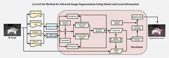
Since most of the conventional level set methods only draw upon the intensity feature, it is easy to get incomplete contours and large quantities of false targets when they are directly applied to process IR images with remarkable intensity inhomogeneity and blurred edges. To solve these challenging problems mentioned above, a new level set method combing global and local information is presented in this paper. First of all, we propose to construct a novel SPF by integrating a global term and a local term together. Specifically speaking, the global term is calculated by the global average intensities inside and outside of the evolving curve. In addition, the local term is constructed by the signed driving force that is associated with four local statistical features: gradient, entropy, standard deviation and filtered difference. Please note that both the direction and magnitude of the driving force are determined by the distances between the feature vector and the two mean multi-feature vectors inside and outside the contour. Then, we use an adaptive weight matrix calculated based on the range value of each pixel to fuse the global and local terms as a hybrid SPF. Next, the level set formula is formed under the framework of GAC model by substituting the edge stopping function with our proposed SPF. Since the presented level set formula takes both global intensity and local multi-features into account, the curve can evolve fast when it is far away from the real boundary meanwhile the evolution is strictly controlled when it is near the object of interest. Besides, a Gaussian convolution is introduced to regularize the level set function so that the re-initialization with high-computational amount can be avoided. By iteration, the curve will evolve to the target boundary until the level set function converges. Figure 1 shows the complete flow chart of our work.
In conclusion, the main contributions and advantages of this study can be summarized as the following aspects:
- a new SPF integrating both global-intensity-based information and local-multi-feature-based information via an adaptive weight matrix is developed;
- four statistical features are dynamically weighted by range ratio to form the driving force which is utilized to form the local term of SPF;
- a level set formula which is able to cope with the weak edge and intensity inhomogeneity is constructed using the SPF proposed;
- the segmentation results are not obviously influenced by the initialization of contour.
The remainder of this paper is organized as follows: in Section 2, the related work in regard to the GAC framework is introduced; in Section 3, the detailed theories of the proposed level set method are depicted; in Section 4, comparisons with other state-of-the-art methods are conducted to verify the superiority of our method; finally, a conclusion is drawn in Section 5.
2. Related Work about Geodesic Active Contour (GAC) Model
Suppose that is a two-dimensional image domain and is a given single channel IR image. Let be a differentiable parameterized curve in . The GAC model is aimed to minimize the following energy functional:
where, is a gradient operator; is the edge stopping function that can be understood as an edge detection function, and its definition is given as
where, represents the arc length of the curve C; means convolving the IR image I using a two-dimensional Gaussian kernel whose standard deviation is . Obviously, satisfies the requirement that the edge stopping function gets the minimum when the curve stops on the boundary; on the contrary, Equation (2) tends to be 1 when the curve is on non-edge regions.
By virtue of the variational theory [31], the Euler-Langrange equation of Equation (1) can be obtained as Equation (3).
where, means the derived function of C; and represent the curvature of the contour and the inward normal to the curve, respectively. In addition, a constant velocity term is employed to increase the propagation speed and Equation (3) can be re-written as:
Furthermore, by representing the closed curve C with the zero level set of the level set function , the corresponding level set formula can be deduced as follows:
where, is also called as the balloon force and it controls the contour expanding or shrinking; stands for the curvature term.
Please note that the contour evolution only depends on the edge information, indicating that the segmentation result of GAC model is easy to be affected by noise and fall into a local minimum when the initial contour is far from the desired object [10]. Motivated by this key point, we consider substituting its edge stopping function with a specific term that contains the global and local information simultaneously. By this means, the new level set model is able to be robust to the adverse interferences existing in IR images.
3. Theory
In this section, the theories regarding the proposed level set method are illustrated at length. In Section 3.1, the way of constructing the SPF is introduced; in Section 3.2, we further depict the implement of this method; at last, a summary of the whole procedure is revealed in Section 3.3.
3.1. Signed Pressure Fucntion Integrating Global and Local Information
As is mentioned in Section 2, one of the key techniques in this study is to design a new SPF containing a global term and a local term to replace the edge stopping function under the GAC framework. According to the previous works about SPF [7,8,32], there are two basic design principles to be noticed: (i) the defined SPF should be in the range ; (ii) the essence of SPF is to modulate the signs of the pressure forces inside and outside the image region. By the guidance of SPF, the contour expands when it is inside the target of interest and shrinks when it is outside the target to be extracted.
3.1.1. Design of the Global Term
The global term of SPF is supposed to make sense when the evolving curve is far away from the object and it provides a powerful force to drive the curve to approach the real boundary with a fast speed. Based on this consideration, the global term needs to focus on the average intensities inside and outside of the curve [7]. Thus, the following definition is adopted:
where, and are two parameters related to the level set function and they stand for the average intensities inside and outside the contour. Equation (6) modulates the signs of the pressure forces inside and outside the region of interest so that the contour shrinks when outside the object and expands when inside the object. The mathematical expressions of and are shown as Equations (7) and (8).
where, is the Heaviside function whose regularized version is selected as:
where, is the inverse tangent function and is a control factor. H(x) can be understood as an approximation of the condition: , if ; , if .
3.1.2. Design of the Local Term
To provide a more precise evolution direction when the curve is in the regions with intensity inhomogeneity or weak edge, local features need to be taken into consideration in the level set method. In this paper, four statistical features: gradient , local entropy , local standard deviation and filtered difference , that can reflect the local property of each pixel are selected to compose a feature vector . In addition, each feature is defined as Equations (10)–(13).
where, is an sized local window set around the center pixel ; L is the maximal gray level of the input IR image ( for an 8-bit image); means the probability of gray level t in , where is the number of pixels whose gray level is t and is the total pixel number in the local window; represents the average intensity in ; is an sized mean filter and means a mean filtering convolution. Here, a further explanation of Equations (10)-(13) is given: is the vector sum of horizontal and vertical gradients, and it reflects the comprehensive gradient of (x, y); and stand for the local entropy and local standard deviation of (x, y) respectively, and they are utilized to measure the local texture of each pixel; is the absolute difference between the original intensity and the intensity processed by mean filtering, and this filtered difference is commonly applied to reflect the local roughness [8].
Next, we argue that the four features in each feature vector should possess different weights according to the degree of inhomogeneity when they are further utilized to calculate the driving force. In light of this consideration, we employ a metric called range ratio [33] to be the adaptive coefficient, and Equation (14) below shows the definition.
where, and denote the maximal and minimal feature values in the local window ; is the maximal pixel value of the whole feature map; stands for the maximal range ratio among the four features and it is utilized for normalization. Thus, a feature weight vector can be obtained for each pixel.
Then, let us focus on studying the construction of driving force which is closely related to the afore-proposed local multi-features. We notice that in LBF model [21], the local intensity information inside and outside the contour is embedded via a Gaussian kernel function used in the energy functional, which is revealed as Equations (15) and (16).
where, and are two values that predict the average intensities inside and outside the contour; is a Gaussian kernel function whose standard deviation is ; and , where is the Heaviside function introduced in Equation (9). For a further understanding of Equations (15,16), and are weighted averages of the intensities in a neighborhood of (x,y), whose size is proportional to the scale parameter [21].
Referring to LBF model, we also embed gradient, local entropy, local standard deviation and filtered difference to our model with a Gaussian kernel function [34,35]. For further emphasizing the local property, the mean operator that computes the mean value in a sized local window is also used to smooth the embedded local feature for each pixel. By this means, each pixel has two mean multi-feature vectors inside and outside the contour. This procedure is mathematically expressed by Equations (17) and (18) and is intuitively depicted by Figure 2.
where, and are the two mean multi-feature vectors inside and outside the contour, and they are composed of four single-feature values denoted as and respectively.
Furthermore, the distances between , and that measure the similarities are computed using the feature weight vector as Equations (19) and (20).
where, represents calculating the absolute value. In essence, and are the weighted sums of the four feature distances, and they indicate the evolving direction of the current pixel . Accordingly, the magnitudes of the driving forces from the two directions can be determined as follows:
where, denote the internal and external driven forces, respectively; is a constant parameter.
By comparing and , the driving force , which is also regarded as the local term of SPF, are computed as Equation (23).
Please note that the driving force indicates both the evolution direction and magnitude for each pixel on the curve.
3.1.3. Combination of Global and Local Terms
After computing the global and local terms using the procedures introduced in Section 3.1.1 and Section 3.1.2, we need to fuse the two terms adaptively and construct a complete SPF. That is to say, the SPF can be written as:
where, is the adaptive weighted coefficient of each pixel, and we call as the adaptive weight matrix in this paper. Equation (24) indicates that whether the SPF in our method is dominated by the global information or the local information is determined by .
As is emphasized above, the intensities in the regions far away from the object vary slowly. As a result, it is unsuitable and unnecessary to use local features to describe these image blocks, i.e., the weight of should increase in these regions. On the contrary, the intensities tend to change drastically, and as well as computed by Equations (7) and (8) may deviate from the real average intensities inside and outside the contour when the curve is in the regions near the boundary of object. In this case, the weight of should increase accordingly. To sum up, the global term plays a dominant role in the smooth regions while the local term becomes extremely significant in the regions with remarkable intensity inhomogeneity.
Similar to the concept of range ratio used in Equation (14), we propose to calculate the range matrix that measures the local roughness as Equation (25).
where, and means computing the maximum and minimum in . To some degree, can be understood as the local contrast of (x,y).
Next, we need to find an appropriate mapping function to establish a mapping relationship between the range matrix and the adaptive weight matrix . Two basic requirements that the mapping function needs to meet are reported below:
- it should be a non-negative and monotonically increasing function;
- and , where and denote the maximum and minimum in the range matrix .
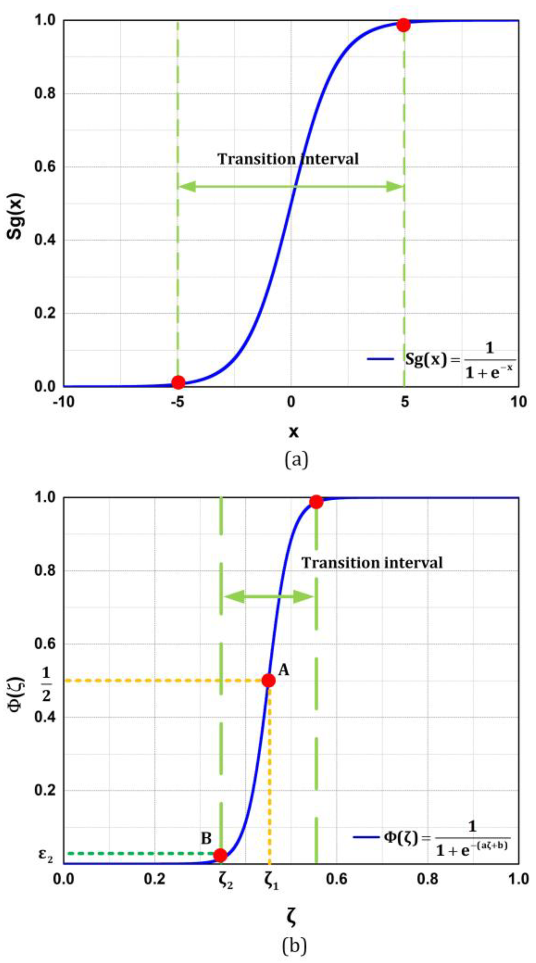
Inspired by the previous work about IR small target enhancement [36], we fortunately find that the standard sigmoid function whose mathematical form is can meet the above two points (see Figure 3a). However, we notice that there is a transition interval in Sg(x) that occupies a large percentage of the whole interval. We argue that the width of this transition interval should be strictly controlled, i.e., corresponding to the central point A and corresponding to the lower inflection point B should be carefully selected (see Figure 3b), because once the relatively smooth area with a small is dominated by the local term of SPF, the evolution of curve will be extremely slow and is easy to drop into local minima. Thus, some modifications in regard to the scale and phase terms are necessary. Suppose that the final mapping function based on the standard sigmoid function is expressed as follows:
where, a and b represent the scale and phase parameters, respectively. As is shown in Figure 3b, these two parameters are determined by the two key points and , where is a constant close to the lower bound 0. By substituting A and B into Equation (26),
where, and in this paper; is a constant which is set by experience.
By this stage, the adaptive weight matrix can be worked out as and the final SPF can be constructed as Equation (24).
3.2. Implementation
Although we have addressed the problem of constructing the SPF fusing global and local information, there are still three aspects that should be noticed in the implementation of the whole algorithm: (i) the initialization of level set function; (ii) the construction of level set formula; (iii) the evolution of level set function.
3.2.1. Initialization of Level Set Function
In our method, the level set function is initialized with a random positive constant using the following formulation:
where, is a positive constant which is set randomly; is a subset of the image domain and denotes the boundary of .
With regards to , it can be set randomly when the level set function is partly controlled by a global term [20]. That is to say, the initial location, shape and size of will not influence the curve evolution obviously in our method. For convenience, we set as an sized square which is located in the center of the input image for all the experiments.
In Section 4, we will further demonstrate that the initialization of the level set function does not influence the segmentation results by experiments.
3.2.2. Construction of Level Set Formula
In this paper, the edge stopping function of the GAC model is replaced by the proposed hybrid SPF for the purpose of dealing with intensity inhomogeneity and blurred edge. Substituting the edge stop function in Equation (5) with the proposed SPF, our level set formula can be expressed using the following formulation:
In Equation (29), the curvature-based term is utilized to regularize the level set function . Since is a signed distance function that satisfies the condition , the regularized term can be expressed by a Laplacian of . As pointed out in the theory of scale-space [37], the evolution of a function with its Laplacian equals to a Gaussian kernel filtering the initial condition of the function [7]. Hence, a Gaussian filter whose standard deviation is can be used to regularize in this study. In this case, the regularize term can be removed from Equation (29). Also, the term is unnecessary because the proposed method uses the statistical information of regions that has a large capture range and capacity of anti-edge leakage [7,8]. Lastly, the level set formula of our method can be written as:
3.2.3. Evolution of Level Set Function
Since the level set formula can be regarded as the derivative between and , the level set function in the t-th iteration can be updated as:
After that, let if ; otherwise, . According to Zhang’s comment [7], this step is alternative, i.e., it is necessary if we want to selectively segment the desired object; otherwise, it is unnecessary.
Moreover, as introduced in Section 3.2.2, a Gaussian kernel filtering is employed to regularize the new level set function as:
where, is the Gaussian kernel utilized whose standard deviation is ; the kernel size is , where is a rounding operator.
By iteration, the evolution of can be regarded as convergent when the current meets the following condition:
where, means calculating the Frobenius norm, is a convergence threshold. In fact, Equation (33) indicates that the level set function does not change obviously any further.
Finally, the zero-level set is selected as the resulting contour .
3.3. Summary of the Proposed Method
To highlight the complete implementation of our method, the main procedures are summarized in Algorithm 1 below according to all the afore-introduced theories.
| Algorithm 1 Level set method using global and local information |
| Input: an IR image |
| 1. Initialization: initialize the level set function to be a binary function using Equation (28). |
| 2. While not convergence do |
| 3. for each pixel do |
| 4. Calculate the global term of SPF using Equation (6) |
| 5. Calculate the local term of SPF using Equation (23) |
| 6. Calculate the adaptive weight matrix using Equation (25) |
| 7. Combing and to construct SPF using Equation (24) |
| 8. end 9. Construct the level set formulation according to Equation (30) |
| 10. Evolve according to Equation (31) |
| 11. Let , if ; otherwise, |
| 12. Regularize using a Gaussian kernel function according to Equation (32) |
| 13. if |
| 14. break |
| 15. end if |
| 16. end |
| Output: The resulting contour . |
4. Experiment and Discussion
In this section, experiments based on real IR test images and relevant discussions are made. In Section 4.1, the value settings of all the parameters utilized in our method are introduced at first; in Section 4.2, comparisons in terms of segmentation results, segmentation precision, running efficiency and influence of contour initialization are made successively. All the experiments are implemented using Matlab 2012b on a PC with a 2.60 GHz INTEL CPU and 4.0 GB installed memory (RAM).
4.1. Parameter Setting
Here, all the parameters involved, as well as the corresponding meanings and their default values are listed in Table 1.
4.1.1. Parameter Description
According to the previous analysis [21], if is too small, the energy functional would fall into a local minimum meanwhile the final contour location may also drift from the ground truth if is too large. Thus, is set as 1.5 which has been proved to be an appropriate choice [7]. The local windows used for computing local entropy, standard deviation, filtered difference, range ratio and the range matrix are uniformly fixed as sized. The window size is usually to , and we set in the simulations. Besides, the standard deviation of the Gaussian filter used for embedding local features is set as which is referred to the related analysis made by Li et al. [21]. Through their analysis based on the results for different values of , this parameter has little influence on the segmentation result. and are two unique parameters used in our study. It can be seen from Equations (21) and (22) that affects the magnitude of the driving force to some extent, and through our repeated experiments, can achieve a robust and satisfactory performance. decides the central point of and also determines the width of the transition interval of indirectly. Strictly speaking, varies for different images. In this paper, we set as a default value which is selected by experience. More analyses about and are presented in Section 4.1.2. is a constant that represents the value of the lower inflection point of , and it will not obviously affect the output of as long as it is close to 0 (usually smaller than 0.0001) [38]. The balloon force is a crucial parameter that directly determines the precision of segmentation and the convergence rate of the level set function. A larger leads to a fast convergence, but it may also generate leakage of boundary. Vice versa. To keep a balance, we set in this study. The constant used for contour initialization only needs to meet the requirement that , so we set according to Zhang’s choice [7]. denotes the size of initial contour and it is set as in our experiments. As a matter of fact, this parameter has little influence on the segmentation results, which is demonstrated in Section 4.2.4. What is more, the standard deviation of the Gaussian filter used for regularizing level set function is also quite important. On the one hand, if the standard deviation is too small, the presented model will be sensitive to noise; on the other hand, false extraction of object and leakage of boundary are easy to happen if it is too large. The empirical value of is in the range [1.5, 3.0], and it is set as in our model. Lastly, the convergence threshold is used as a stop condition of the curve evolution and Equation (33) indicates that the level set function tends to be constant at t-th iteration. Based on this consideration, should be a constant close to 0 and we find that the resulting curve has no remarkable changes any more when the rate of change of is smaller than 3%.
4.1.2. Sensitivity Analysis
In this section, we focus on discussing the sensitivities of two significant parameters and so as to obtain their suitable settings. As mentioned in Section 4.1.2, the default values of other parameter are selected according to the previous studies, so we do not discuss them again.
Here, F value [39,40] is employed as a measuring metric for sensitivity analysis. The define of F value is given as follows:
where, is a harmonic coefficient and in this paper; P and R denote the precision rate and recall rate respectively, which are defined as:
where, represents the area extracted by the level set method; represents the object region provided by the ground truth; represents the correctly segmented region, i.e., . For an intuitive illustration, Figure 4 provides a schematic diagram to show relationship between , and . Obviously, a larger F value indicates a more accuracy segmentation result, and F is in the range .
We consider that an appropriate parameter setting of or need to get higher F values in most of the practical IR scenes. Here, 6 typical IR images shown in Figure 5 are utilized to make the sensitivity analysis, in which we continuously change the values of or while other parameters are fixed with the default values listed in Table 1.
A statistic of F values with different is implemented. changes from 0.1 to 5 (the step length is chosen as 0.1) and the presented algorithm is conducted to produce a resulting segmentation image for each , after which the corresponding F value is calculated. For , the same procedure is adopted to obtain the statistic of F values. In our simulation, varies from 0.01 to 1 and the step length is set as 0.02. By this means, we can get 50 groups of data for each parameter and the following two cartograms drawn in Figure 6 reveal the sensitivities of and respectively.
As for , it does influence the segmentation accuracy significantly since the -sensitivity curves shown in Figure 6a undergo striking fluctuations in most scenes. However, we find that the F values can keep in high levels when is in the range and the statistical results are relatively stable. To this end, we adopt for all the experiments.
It can be seen from Figure 6b that the -sensitivity curves increase rapidly before and level off after . As far as we are concerned, the level set function is dominated by the local term when while it is dominated by the global term when . To keep a balance, we set in this paper.
We would like to state that the specific values of the parameters involved in this study may still need to be adjusted in different cases so as to get more accuracy segmentation results (especially , and ), and the values provided in Section 4.1 are just default values.
4.2. Comparative Experiment
In this part, 6 state-of-the-arts level set methods: GAC [9], CV [15], SBGFRLS [20], LBF [21], ILFE [22], Cao’s model [8] and an interactive segmentation method: MSRM [28] that all have been discussed in Section 1 are selected to make both qualitative and quantitative comparisons with the method proposed in this paper. In Section 4.2.1, the level-set-based algorithms are tested with a uniform initial contour while MSRM is conducted with the object and background markers being added artificially. Then, two metrics indicating the segmentation precision are employed to evaluate the segmentation results in Section 4.2.2. Next, comparisons in terms of running time and iterations are made in Section 4.2.3. Finally, an additional experiment to test the influence of contour initialization is implemented in Section 4.2.4.
4.2.1. Segmentation Result
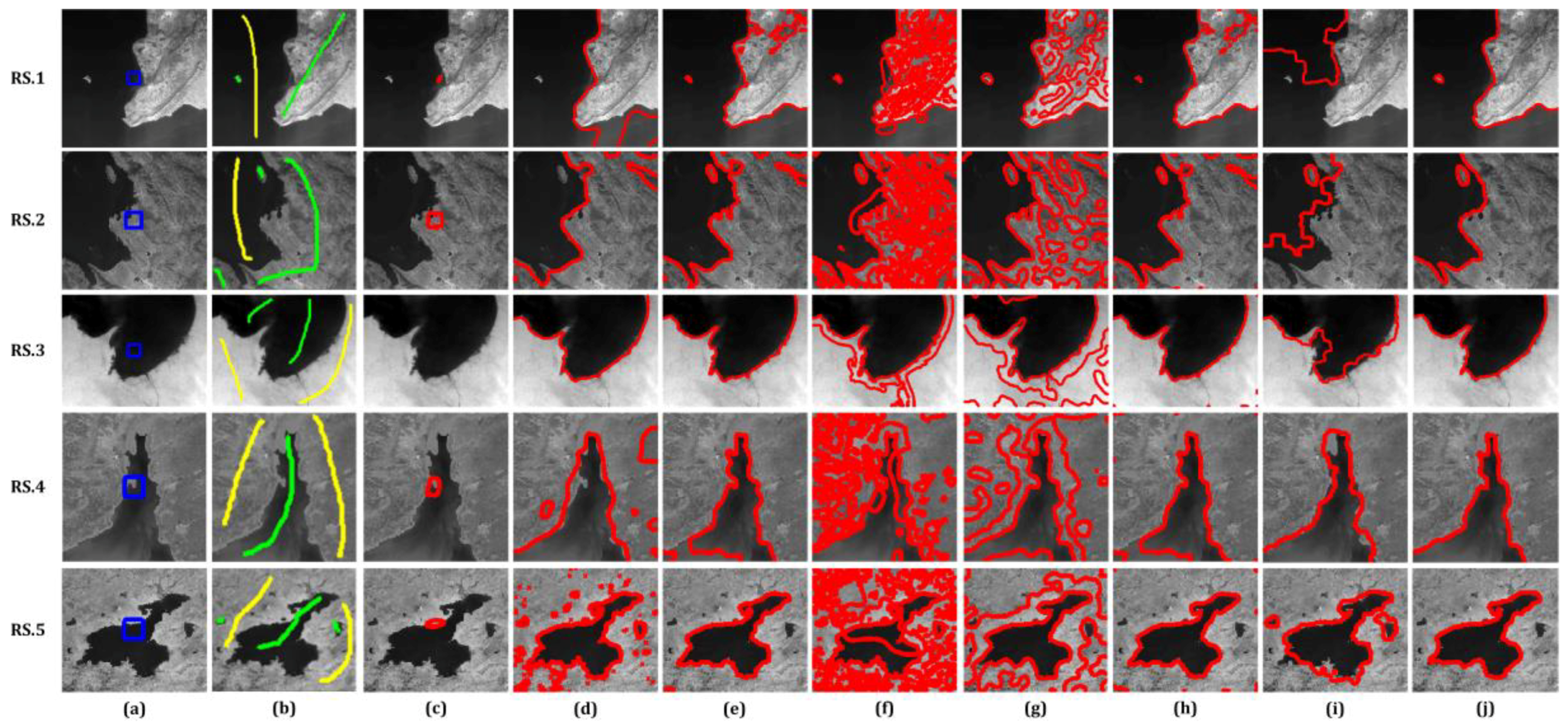
In this section, apart from 30 IR images (part of them can be downloaded from Ref. [41]), 5 natural images [42] and 5 remote sensing images [43] are also adopted to be the database in order to verify that the proposed algorithm is general.
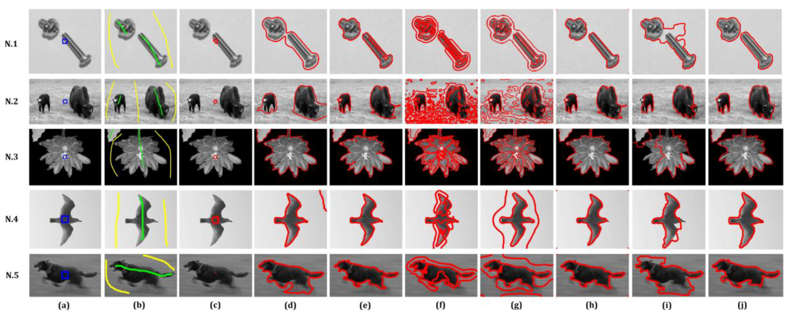
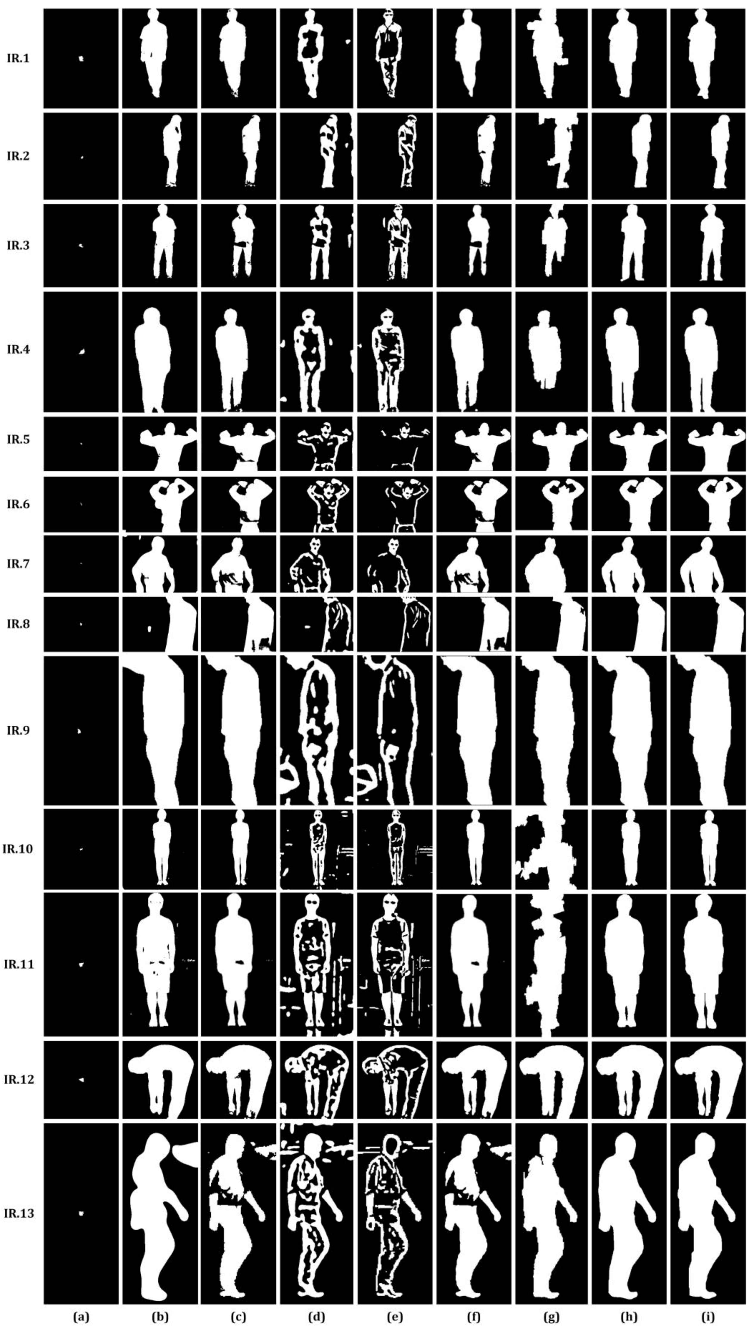
Figure 7, Figure 8 and Figure 9 report the segmentation results of IR images, natural images and remote sensing images respectively. The IR images utilized can be classified into two categories: single-object-images and multiple-object-images, and they all contain blurred object boundaries and a degree of local intensity inhomogeneity. In particular, test images, like IR.10 and IR.11 in Figure 7a, are contaminated by noises and the disturbances of false alarm (e.g., edges of the cart and laboratory furniture) are quite obvious. The target/background contrasts of the natural images and remote sensing images are higher and the details, especially the edges and textures, are richer.
For a fair comparison, we use a uniform initial contour to define the binary level set function for each test image, which can be seen from the blue rectangle in the first columns of Figure 7, Figure 8 and Figure 9. Also, the initial object and background markers of MSRM, which are marked in green and blue, are shown in the second columns. In addition, the 3–8 columns correspond to the segmentation results of GAC, CV, SBGFRLS, LBF, ILFE, Cao’s model, MSRM and our method, respectively. Please note that the final evolving curves are marked in red.
As is introduced above, GAC model is highly dependent on the initialization of contour, and it can only get complete segmentation results when the initial contour contains the whole object of interest. In this comparative experiment, the initial contour is set in the image center and most of the objects are partly covered. As a result, the contours evolved by GAC model all converge to local minima, which leads to the seriously incomplete segmentations. More seriously, the curve totally disappears if the initial contour is far away from the object (see IR. (20, 23) in Figure 7c and RS. 3 in Figure 9c).
Chen-Vese (CV) model draws upon the statistical intensity information to evolve the curve and is able to achieve satisfactory performances in binary phase segmentation. Basically speaking, all the objects are extracted by CV model, but boundary leakage occurs in those inhomogeneous areas due to the fact that this model is established with the assumption that image intensities in each region always maintain constant. For example, as can be seen from IR. (1, 7, 11, 14) in Figure 7d, some striking holes on the clothes are mistakenly generated in the final segmentation results. Moreover, CV model is quite sensitive to the disturbance of noise, which can be demonstrated by the fake targets on the cart and ground in IR. (10, 11) in Figure 7d. Besides, we find that the convergence of CV model is quite unstable, e.g., IR. (18, 20, 26, 29) in Figure 7d, which we infer may be associated with the contour initialization.
In regard to SBGFRLS model, it also does well with IR images with homogeneous intensities, e.g., IR. (18, 20, 26, 29) in Figure 7e and natural images, but its performance turns to be bad when dealing with inhomogeneous cases. From our experiments, we can clearly find that incompleteness of segmentation always occurs near the borders between the object and the ground, the cloth parts of humans in IR images (see IR. (3, 5–8, 14) in Figure 7e) and the lands in remote sensing images (see RS. (1, 2, 4) in Figure 9e), because the intensity distributions of these regions are quite uneven, which causes severe interferences for the expansion or shrink of the contour.
Additionally, it is obvious that LBF and ILFE get a large number of false targets when coping with images with rich texture information. On the one hand, many edges belonging to the background are recognized as the real boundaries in IR. (10, 11) in Figure 7f and Figure 7g; on the other hand, the real object is divided into too many blocks, which absolutely cannot satisfy the visual requirement of image segmentation. It should be noticed that the initial contour has an outstanding influence on the results of ILFE, since there is a remarkable false target with a relatively large area around the position of the initial contour in IR. (20, 21, 26, 27) in Figure 7g.
Cao’s model takes full advantages of global and local intensity information, so it can successfully address the weak edges and local intensity inhomogeneities. As a whole, Cao’s method is able to extract the objects in all the test images, although there are still some incompleteness existing in the final contours, especially in the feet and clothes parts, which can be seen from IR. (3, 5–8, 13, 14) in Figure 7h. We notice that its performances in remote sensing images are not satisfactory enough and there are several false segmentations existing in RS. (1, 2) in Figure 9h, while the segmentation results are almost perfect in natural images. From our point of view, this is mainly because that the local term of Cao’ model that only takes intensity information into account is still not robust to complex texture patterns.
Maximal similarity-based region merging (MSRM) method is an interactive image segmentation that guides the region merging with the aid of two kinds of markers. Although the fore-and-background markers are correctly provided, we notice that the object boundaries obtained still deviate from the ground truth in some cases, especially in IR images, such as IR. (1–3, 10–11, 18, 27) in Figure 7i. Intuitively, those inaccurate boundaries are lack of smoothness and many background image patches are mistakenly classified into the foreground class. In our opinion, there are two main reasons that lead to the segmentation errors: (i) the rough segmentation using mean shift or super-pixel is always inaccurate in gray images; (ii) IR images are lack of color and texture information, so the similarities between each region are not convincing.
Fortunately, our method obtains the most complete and precise segmentation results among the 8 algorithms owing to its strategy of integrating the average intensity-based global information and multi-feature-based local information. As can be seen from IR. (1–3, 28) in Figure 7j, the feet are perfectly picked out and the problem of boundary leakage does not occur in our method. Also, the interferences of noise and edge in IR. (10, 11) in Figure 7j do not take any effects on the final results. Thus, we argue that the superiority of the proposed method is proved by this comparative experiment. On the other hand, our method is somewhat weak at dealing with tiny objects, e.g., the ox horn in N. 2 in Figure 8j and the small circle-shape land in RS. 5 in Figure 9j are lost, and the fluorescent lamp in IR. 18 is mistakenly recognized as the object.
4.2.2. Comparison of Segmentation Accuracy
To further prove the superiority of our method, we would like to compare the precision of segmentation results through a quantitative way. First of all, the segmentation results shown in Figure 7, Figure 8 and Figure 9 are transferred to binary maps according to the corresponding final level set functions. Figure 10, Figure 11 and Figure 12 display the binary maps as well as the ground truth, respectively.
As is introduced in Equation (34), F value is extensively employed to measure the segmentation accuracy in the field of object detection. Here, Table 2 lists the corresponding F values of all the binary segmentation maps in Figure 10, Figure 11 and Figure 12 and the average F value of each algorithm is given in the last row. The top two F values in each group are marked with bold values.
Apart from F values that indicate the overlapping rate, another metric called boundary precision (BP) that evaluates ability of precise boundary locating [27] is also applied to make quantitative comparisons in this section. Below, the definition of BP is given as:
where, u and v are the pixels on the result boundary and ground-truth boundary; and denote the number of pixels on the corresponding boundaries; for each pixel u, means the minimal distance between u and the pixels on the ground-truth boundary; similarly, for each pixel v, means the minimal distance between v and the pixels on the result boundary. Obviously, a higher BP refers to a more accuracy boundary locating.
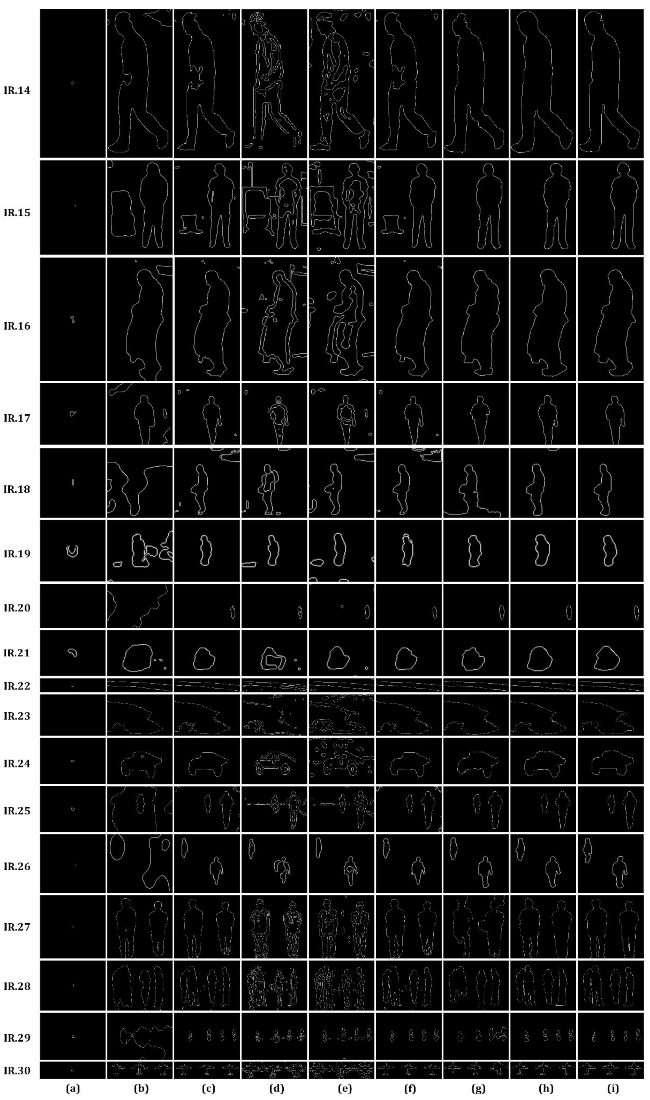
Figure 13, Figure 14 and Figure 15 reveal the boundary maps extracted by Sobel algorithm [44] and the ground-truth boundaries. Table 3 reports the BP value of each test group clearly.
As is revealed from Table 2, our method achieves the largest F values on average (96.04%) while GAC model always gets the worst F values in all the test images. GAC model is an edge-based level set method, so its segmentation results are poor if the initial contour cannot totally contain the real object. In our case, the initial contour is set as a rectangle located in the image center which partly covers the object. Hence, the segmentation precision is doomed to be very low. LBF model and ILFE model excessively concentrate on the local intensity feature, but they ignore the global intensity instead. Although this strategy can extract the details in a cautious way, it may result in too many segmented blocks in the object region and cause large quantities of false targets in the background. That is the main reason their F values basically maintain around 50–60%. SBGFRLS model is able to partition the objects well, but it cannot do in addressing the details perfectly. When the evolving curve approaches the boundary, the further evolution becomes inaccuracy due to the fact that the regions near the boundary are always inhomogeneous, which does not accord with the assumption of this model. That is to say, the average intensities inside and outside the contour estimated by Equations (7) and (8) are distorted. As a result, it is difficult for SBGFRLS to achieve F values greater than 95%. CV model’s robustness to local intensity inhomogeneities is stronger than SBGFRLS model, but the it cannot avoid causing false segmentations inside the object. This drawback is reflected by those minor holes on the human bodies. Also, the disturbances of noise decrease the F values of CV model to some extent. The F values of Cao’s model are around 92% which are approximately on the same level of SBGFRLS model, but the average value is decreased by its weak performance in a small part of the test images, such as IR. (18, 26) in Figure 10. To further analyze, we consider that it may be the inaccuracy of its weight function used to integrate the global and local terms that results in the striking boundary leakage, indicating that its robustness needs to be improved further. With the help of makers, MSRM achieves relatively high F values, even higher than our method in certain test images. We think it is quite reasonable because the additional makers do provide much useful information for MSRM to distinguish between objects and backgrounds. The average F value of our method is about 4.5% higher than the second place (SBGFRLS), and our method gets the top largest F values in almost all the database. Through observing the binary segmentation results, we find that our method possesses an outstanding ability to overcome the problem of boundary leakage and it is much less sensitive to the noise, which guarantees its high segmentation precision. However, we still need to point out that the segmentation errors of the proposed method are mainly derived from the miss of groove parts (e.g., the inner thigh).
The overall distribution of BP value depicted in Table 3 is almost the same as F value, i.e., our proposed level set method generally outperforms other comparing algorithms in terms of boundary precision (0.8575 on average) while the BPs of GAC model are far smaller than others (only 0.0219 on average). This phenomenon matches the statistical result of F values quite well, proving that the conclusions derived from these two metrics are both convincing. It is interesting that MSRM often gets the top two best BPs among the IR image database, but SBGFRLS models takes the second place on average. This phenomenon indicates that SBGFRLS model is more robust than MSRM method and it can keep in a relatively high boundary locating level as well. CV, LBF and ILFE absolutely do not have strong boundary locating abilities according to Table 3. For CV model, the weak and unstable convergence decreases it overall BPs to a great extent while the large quantities of false boundaries caused by LBF and ILFE models weaken their BPs sharply. The performance of Cao’s model is moderate among all the 8 algorithms. There are no severe segmentation errors, but the BPs cannot be improved further since the leakage of boundary is still not solved.
4.2.3. Comparison of Running Time
As is commonly known, running speed is also a significant factor in evaluating an algorithm. In this section, we test the number of iterations (except MSRM) and the execution time respectively, which are listed in Table 4 and Table 5.
With respect to the number of iterations, it can be clearly observed from Table 4 that our method has the fewest iterations in most of the test images (fewer than 50 times), which demonstrates its best convergence among all the other methods. We consider that its outstanding convergence is mainly owing to the fact that the average intensity-based global term accelerates the evolving speed meanwhile the local multi-feature-based term avoids the energy functional falls into local minima. SBGFRLS, LBF and Cao’s models also achieve relatively satisfactory iteration times which maintain around 50 times on the whole. However, we notice that the convergences of SBGFRLS model and Cao’s method become poor when dealing with IR. 10 that contains several edge disturbances. This phenomenon indicates that these two models would still drop into local minima when facing the complex scenes. When compared with the afore-discussed methods, CV and ILFE models turn to be relatively weak in iterations. Since CV model does not contain any local intensity information, the evolution of curve may slow down in inhomogeneous regions. For ILFE model, the Laplacian fitting term may have an adverse effect on the convergence also. Lastly, GAC model is the worst one whose iterations are more than 10 times than the proposed method. As has been discussed above, its curve evolution is easy to stagnate around the initial contour if the initialization itself is set inappropriately.
When considering the whole execution time, it can be seen from Table 5 that those level set methods that only involve global intensity information, e.g., GAC, CV and ILFE, get relatively fast running speeds. Among them, although GAC and CV suffer from large numbers of iterations, their whole running time is still shorter than SBGFRLS and Cao’s model owing to its high efficiency of the single iteration. The total running time of LBF is also fine, but it is because of its few iterations, rather than the single iteration efficiency. MSRM gets the fastest execution speed among all the 8 algorithms, because this method does not have the problem of convergence and the user’s interaction time is not included in our test. Our method achieves the moderate performance in this comparison, meaning that the running efficiency is not the best. As far as we are concerned, it is the procedures of calculating the multi-features and constructing the driving forces inside and outside the contour that increase the running time. Thus, it is of great necessity for us to adopt the parallel processors, e.g., FPGA and GPU, and optimize the codes further.
4.2.4. Influence of Contour Initialization
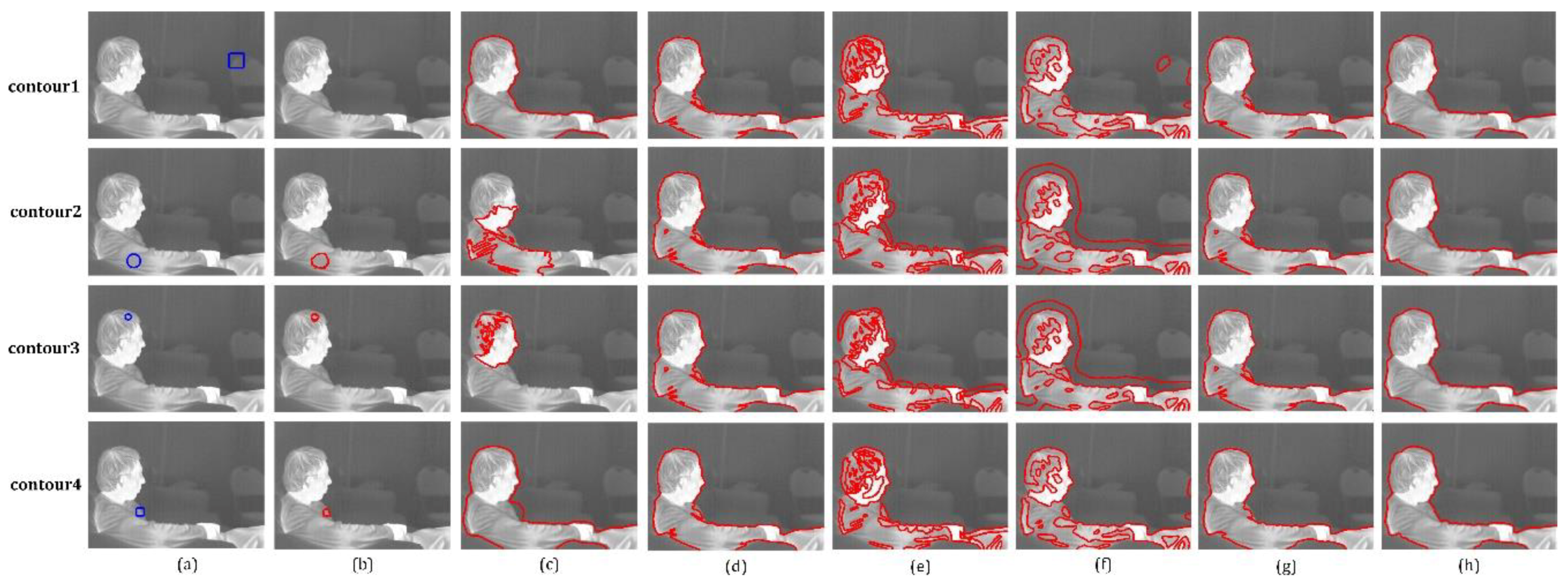
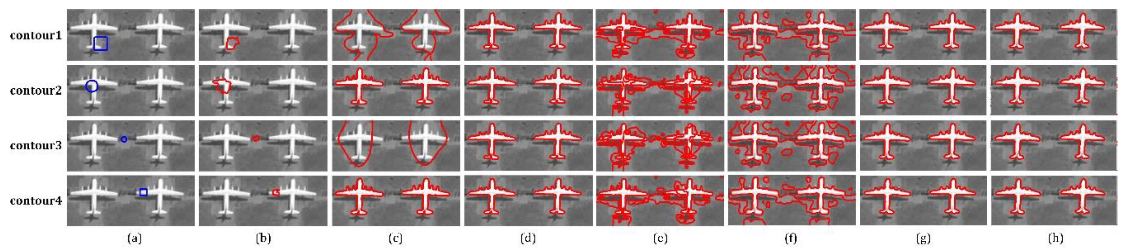
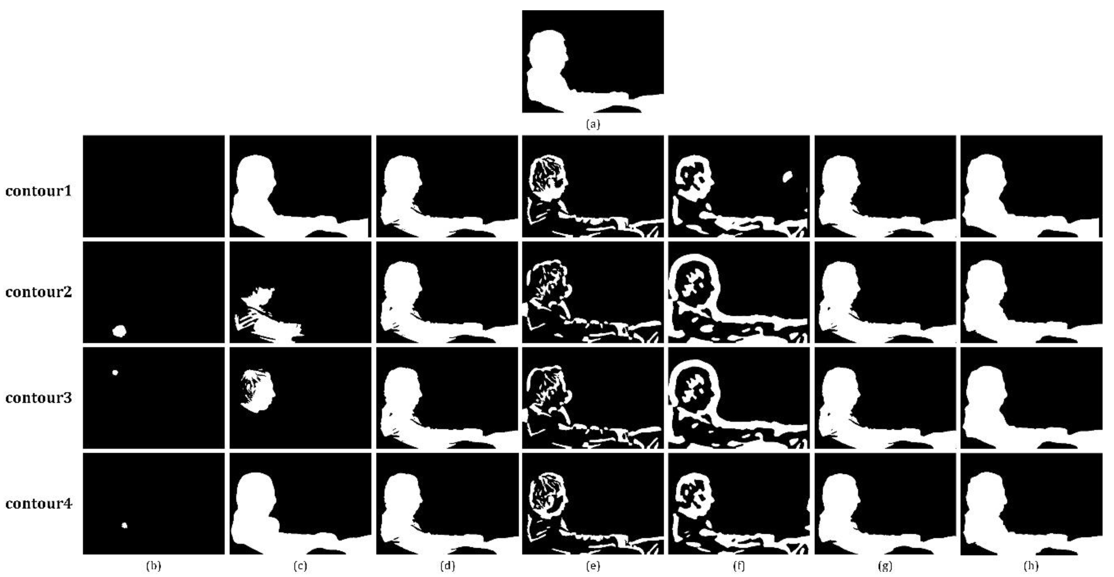
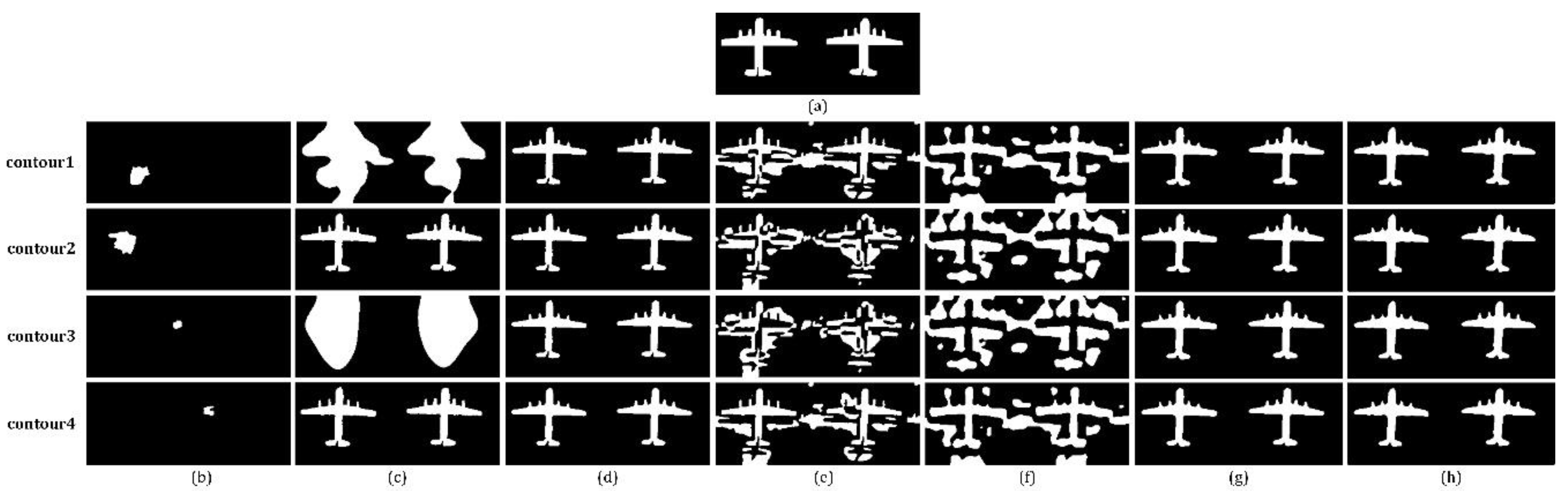
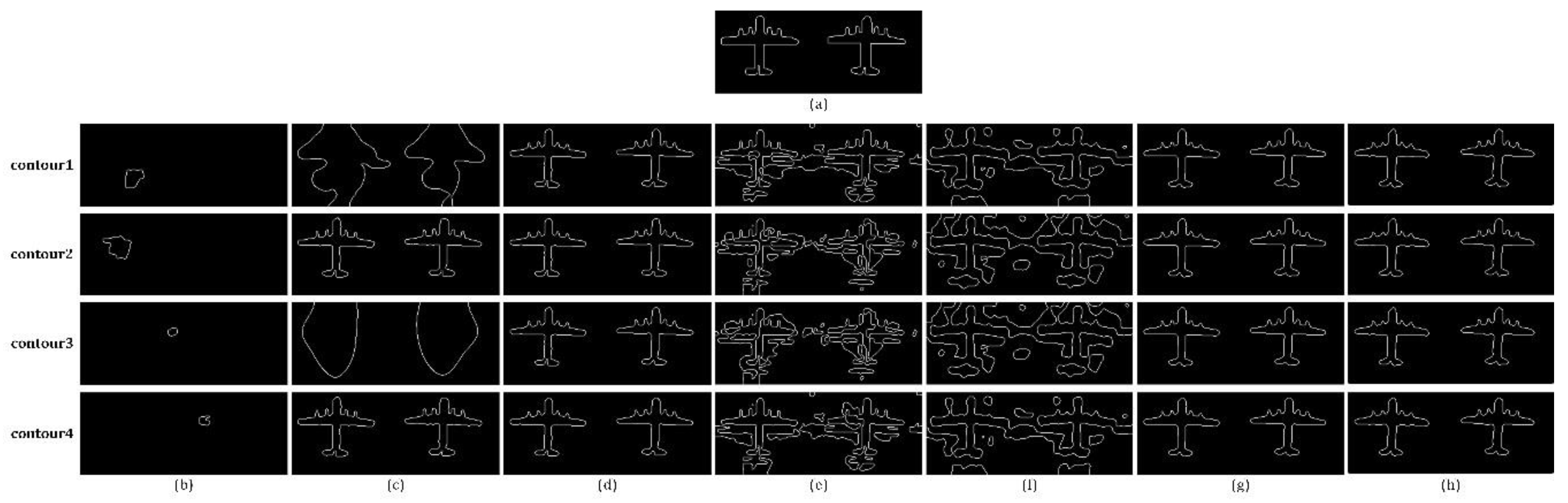
As is extensively acknowledged that an excellent level set method needs to be robust to the initialization of contour. Based on this consideration, an additional experiment aimed to test the influence of contour initialization on the final segmentation results is implemented in this section. As is shown in Figure 16 and Figure 17, two groups of IR images (called ‘man’ and ‘plane’) are used and the initial contour is set as four different conditions. The corresponding binary maps and boundary maps are presented in Figure 18, Figure 19, Figure 20 and Figure 21. Also, the F values and BP values are listed in Table 6 and Table 7.
Here, three key points: position, size and shape, are considered by us. For both Figure 16 and Figure 17, the initial positions of contours can be classified as inside the object, outside the object, partly inside the object; the initial sizes of contours can be classified as and ; the initial shapes can be classified as square and circle.
Intuitively speaking, the initialization of contour has little effect on SBGFRLS, Cao’s model and the proposed method according to our experiment. As is reported in Table 6 and Table 7, the Fs and BPs of our method and Cao’s model are still superior to other comparing algorithms while those of SBGFRLS are moderate. In general, the utilized metrics of the three methods do not undergo remarkable fluctuations. By contrast, the segmentation results of GAC model are seriously affected by the initial contours. On the one hand, it is highly possible for the contour to converge towards the position where its initial condition locates; besides, it is even possible to be absorbed completely if the initial contour has no overlaps with the object. Although the performances of LBF and ILFE still keep in a low level in terms of the two metrics, we still notice that different shapes of initial curve will result in different evolving curves. As is shown in contour 2, 3 of Figure 17, the head part of ‘man’ image will be segmented into fewer blocks by LBF and a striking false contour around the head part will be generated by ILFE when the initial contour is circle. In addition, as we can see in contour 2, 3 of Figure 16 and contour 2, 4 of Figure 17, the curves of CV model stop evolving if it is initialized in a region suffering from intensity inhomogeneity seriously. Accordingly, its Fs and BPs both occupy wide ranges, varying from 0.34–0.96 and 0.06–0.97 respectively.
5. Conclusions
5.1. Methdology
In this paper, a new level set method fusing average-intensity-based global information and multi-feature-based local information is proposed to segment IR images. Different from the conventional level set methods that only consider single intensity feature, the presented model constructs a hybrid SPF made up of a global term and a local term. The global term is calculated based on the average intensities inside and outside the contour while the local term is represented by the driving force computed by four weighted local features. To keep a balance, the two terms are combined via an adaptive weight matrix. By substituting the edge stopping function in GAC model with the proposed SPF, the level set formula is constructed and the level set function is re-initialized by a Gaussian filtering. By iteration, the final contour of object can be obtained and the object is thus extracted. Both qualitative and quantitative experiments verify that our method outperforms other state-of-the-art level set methods in terms of segmentation accuracy, convergence and robustness to contour initialization.
5.2. Applicability and Limitation to Remote Sensing
IR imaging belongs to one of the significant branches of remote sensing and IR image segmentation is extensively applied in many remote sensing applications, e.g., intelligent urban surveillance, unmanned aerial vehicles, pedestrian detection, etc. Although the proposed level set method is aimed to cope with the blurred boundary, low contrast and intensity inhomogeneity in IR image, it can also be directly applied to process remote sensing images when they are converted to single channel images, which has been demonstrated in Section 4.2.1. However, the color and spectrum information of remote sensing images are not fully used when they are processed using our method, indicating that the inherent advantages are ignored. On the other hand, we find that remote sensing images usually contain rich texture information, but the proposed algorithm is somewhat weak at coping with the tiny objects, especially the small circular holes existing in the land. We infer it is the Gaussian filtering used for regularizing the level set function that removes these details.
5.3. Future Work
In the future work, we plan to further optimize the codes of our algorithm and try to transplant the Matlab codes to parallel hardware, e.g., FPGA and GPU, so that the whole computational time can be reduced greatly and the real-time running can be expected. Besides, we notice that the target of interest in IR image can be seen as a salient object, so its visual saliency may be exploited for further investigation.
Author Contributions
M.W. conceived of, designed and performed the algorithm, analyzed the data and wrote the paper; G.G., J.S. and X.M. are the research supervisors; K.R. helped modify the language; W.Q. and Q.C. also provided technical assistance to the research; The manuscript was discussed by all the co-authors.
Funding
This paper is financially supported by the National Natural Science Foundation of China (61675099), the National Natural Science Foundation of China (61701233), Open Foundation of State Key Laboratory of Networking and Switching Technology (Beijing University of Posts and Telecommunications) (SKLNST-2016-2-07), Canada Research Program, and China Scholarship Council.
Conflicts of Interest
The authors declare no conflict of interest.
References
- Huang, J.; Ma, Y.; Zhang, Y.; Fan, F. Infrared image enhancement algorithm based on adaptive histogram segmentation. Appl. Opt. 2017, 56, 9686–9697. [Google Scholar] [CrossRef] [PubMed]
- Zingoni, A.; Diani, M.; Corsini, G. A Flexible Algorithm for Detecting Challenging Moving Objects in Real-Time within IR Video Sequences. Remote Sens. 2017, 9, 1128. [Google Scholar] [CrossRef]
- Lei, S.; Zou, Z.; Liu, D.; Xia, Z.; Shi, Z. Sea-land segmentation for infrared remote sensing images based on superpixels and multi-scale features. Infrared Phys. Technol. 2018, 91, 12–17. [Google Scholar] [CrossRef]
- Wan, M.; Gu, G.; Qian, W.; Ren, K.; Chen, Q.; Maldague, X. Particle swarm optimization-based local entropy weighted histogram equalization for infrared image enhancement. Infrared Phys. Technol. 2018, 91, 164–181. [Google Scholar] [CrossRef]
- Pal, N.R.; Pal, S.K. A review on image segmentation techniques. Pattern Recognit. 1993, 26, 1277–1294. [Google Scholar] [CrossRef]
- Lee, L.K.; Liew, S.C.; Thong, W.J. A review of image segmentation methodologies in medical image. In Advanced Computer and Communication Engineering Technology; Springer: New York, NY, USA, 2015; pp. 1069–1080. [Google Scholar]
- Niu, S.; Chen, Q.; de Sisternes, L.; Ji, Z.; Zhou, Z.; Rubin, D.L. Robust noise region-based active contour model via local similarity factor for image segmentation. Pattern Recognit. 2017, 61, 104–119. [Google Scholar] [CrossRef]
- Cao, J.; Wu, X. A novel level set method for image segmentation by combining local and global information. J. Mod. Opt. 2017, 64, 2399–2412. [Google Scholar] [CrossRef]
- Caselles, V.; Kimmel, R.; Sapiro, G. Geodesic active contours. Int. J. Comput. Vis. 1997, 22, 61–79. [Google Scholar] [CrossRef]
- Tian, Y.; Duan, F.; Zhou, M.; Wu, Z. Active contour model combining region and edge information. Mach. Vis. Appl. 2013, 24, 47–61. [Google Scholar] [CrossRef]
- Melonakos, J.; Pichon, E.; Angenent, S.; Tannenbaum, A. Finsler active contours. IEEE Trans. Pattern Anal. Mach. Intell. 2008, 30, 412–423. [Google Scholar] [CrossRef] [PubMed]
- Paragios, N. Variational methods and partial differential equations in cardiac image analysis. In Proceedings of the IEEE International Symposium on Biomedical Imaging: Nano to Macro, Arlington, VA, USA, 15–18 April 2004; pp. 17–20. [Google Scholar]
- Wang, D.; Zhang, T.; Yan, L. Fast hybrid fitting energy-based active contour model for target detection. Chin. Opt. Lett. 2011, 9, 071001-071001. [Google Scholar] [CrossRef]
- Zhao, W.; Xianze, X.; Zhu, Y.; Xu, F. Active contour model based on local and global Gaussian fitting energy for medical image segmentation. Opt. Int. J. Light Electron. Opt. 2018, 158, 1160–1169. [Google Scholar] [CrossRef]
- Chan, T.F.; Vese, L.A. Active contours without edges. IEEE Trans. Image Process. 2011, 10, 266–277. [Google Scholar] [CrossRef] [PubMed]
- Mumford, D.; Shah, J. Optimal approximations by piecewise smooth functions and associated variational problems. Commun. Pure Appl. Math. 1989, 42, 577–685. [Google Scholar] [CrossRef] [Green Version]
- Wang, Y.; Huang, T.Z.; Wang, H. Region-based active contours with cosine fitting energy for image segmentation. J. Opt. Soc. Am. A Opt. Image Sci. Vis. 2015, 32, 2237–2246. [Google Scholar] [CrossRef] [PubMed]
- Tsai, A.; Yezzi, A.; Willsky, A.S. Curve evolution implementation of the Mumford-Shah functional for image segmentation, denoising, interpolation, and magnification. IEEE Trans. Image Process. 2001, 10, 1169–1186. [Google Scholar] [CrossRef] [PubMed]
- Vese, L.A.; Chan, T.F. A multiphase level set framework for image segmentation using the Mumford and Shah model. Int. J. Comput. Vis. 2002, 50, 271–293. [Google Scholar] [CrossRef]
- Zhang, K.; Zhang, L.; Song, H.; Zhou, W. Active contours with selective local or global segmentation: A new formulation and level set method. Image Vis. Comput. 2010, 28, 668–676. [Google Scholar] [CrossRef]
- Li, C.; Kao, C.Y.; Gore, J.C.; Ding, Z. Minimization of region-scalable fitting energy for image segmentation. IEEE Trans. Image Process. 2008, 17, 1940–1949. [Google Scholar] [PubMed]
- Zhang, K.; Xu, S.; Zhou, W.; Liu, B. Active contours based on image Laplacian fitting energy. Chin. J. Electron. 2009, 18, 281–284. [Google Scholar]
- Wang, L.; Pan, C. Robust level set image segmentation via a local correntropy-based K-means clustering. Pattern Recognit. 2014, 47, 1917–1925. [Google Scholar] [CrossRef]
- Wang, L.; Li, C.; Sun, Q.; Xia, D.; Kao, C.Y. Active contours driven by local and global intensity fitting energy with application to brain MR image segmentation. Comput. Med. Imaging Graph. 2009, 33, 520–531. [Google Scholar] [CrossRef] [PubMed]
- Dong, F.; Chen, Z.; Wang, J. A new level set method for inhomogeneous image segmentation. Image Vis. Comput. 2013, 31, 809–822. [Google Scholar] [CrossRef]
- Zhao, Y.; Nie, X.; Duan, Y.; Huang, Y.; Luo, S. A benchmark for interactive image segmentation algorithms. In Proceedings of the IEEE Workshop on Person-Oriented Vision (POV), Kona, HI, USA, 7 January 2010; pp. 33–38. [Google Scholar]
- Panagiotakis, C.; Papadakis, H.; Grinias, E.; Komodakis, N.; Fragopoulou, P.; Tziritas, G. Interactive image segmentation based on synthetic graph coordinates. Pattern Recognit. 2013, 46, 2940–2952. [Google Scholar] [CrossRef]
- Ning, J.; Zhang, L.; Zhang, D.; Wu, C. Interactive image segmentation by maximal similarity based region merging. Pattern Recognit. 2010, 43, 445–456. [Google Scholar] [CrossRef]
- Veksler, O. Star shape prior for graph-cut image segmentation. In Proceedings of the European Conference on Computer Vision, Marseille, France, 12–18 October 2008; pp. 454–467. [Google Scholar]
- Gulshan, V.; Rother, C.; Criminisi, A.; Blake, A.; Zisserman, A. Geodesic star convexity for interactive image segmentation. In Proceedings of the IEEE Conference on Computer Vision and Pattern Recognition (CVPR), San Francisco, CA, USA, 13–18 June 2010; pp. 3129–3136. [Google Scholar]
- Zhi, X.H.; Shen, H.B. Saliency driven region-edge-based top down level set evolution reveals the asynchronous focus in image segmentation. Pattern Recognit. 2018, 80, 241–255. [Google Scholar] [CrossRef]
- Xu, C.; Yezzi, A.; Prince, J.L. On the relationship between parametric and geometric active contours. In Proceedings of the IEEE Conference Record of the Thirty-Fourth Asilomar Conference on Signals, Systems and Computers, Pacific Grove, CA, USA, 29 October–1 November 2000; pp. 483–489. [Google Scholar]
- Yu, Y.; Zhang, C.; Wei, Y.; Li, X. Active contour method combining local fitting energy and global fitting energy dynamically. In Proceedings of the International Conference on Medical Biometrics, Hong Kong, China, 28–30 June 2010; pp. 163–172. [Google Scholar]
- Wan, M.; Gu, G.; Qian, W.; Ren, K.; Chen, Q. Hybrid active contour model based on edge gradients and regional multi-features for infrared image segmentation. Opt. Int. J. Light Electron. Opt. 2017, 140, 833–842. [Google Scholar] [CrossRef]
- Zhang, T.; Han, J.; Zhang, Y.; Bai, L. An adaptive multi-feature segmentation model for infrared image. Opt. Rev. 2016, 23, 220–230. [Google Scholar] [CrossRef]
- Wan, M.; Gu, G.; Qian, W.; Ren, K.; Chen, Q. Infrared small target enhancement: Grey level mapping based on improved sigmoid transformation and saliency histogram. J. Mod. Opt. 2018, 65, 1161–1179. [Google Scholar] [CrossRef]
- Perona, P.; Malik, J. Scale-space and edge detection using anisotropic diffusion. IEEE Trans. Pattern Anal. Mach. Intell. 1990, 12, 629–639. [Google Scholar] [CrossRef] [Green Version]
- Wan, M.; Gu, G.; Qian, W.; Ren, K.; Chen, Q.; Maldague, X. Infrared Image Enhancement Using Adaptive Histogram Partition and Brightness Correction. Remote Sens. 2018, 10. [Google Scholar] [CrossRef]
- Mangale, S.A.; Khambete, M.B. Approach for moving object detection using visible spectrum and thermal infrared imaging. J. Electron. Imaging 2018, 27. [Google Scholar] [CrossRef]
- Peng, H.; Li, B.; Ling, H.; Hu, W.; Xiong, W.; Maybank, S.J. Salient object detection via structured matrix decomposition. IEEE Trans. Pattern Anal. Mach. Intell. 2017, 39, 818–832. [Google Scholar] [CrossRef] [PubMed]
- Database Collection of Infrared Image. Available online: http://www.dgp.toronto.edu/nmorris/IR/ (accessed on 16 June 2018).
- MSRA10K Salient Object Database. Available online: http://mmcheng.net/msra10k/ (accessed on 19 June 2018).
- Gu, Y.; Ren, K.; Wang, P.; Gu, G. Polynomial fitting-based shape matching algorithm for multi-sensors remote sensing images. Infrared Phys. Technol. 2016, 76, 386–392. [Google Scholar] [CrossRef]
- Gao, W.; Zhang, X.; Yang, L.; Liu, H. An improved Sobel edge detection. In Proceedings of the 2010 3rd IEEE International Conference on Computer Science and Information Technology (ICCSIT), Chengdu, China, 9–11 July 2010; pp. 67–71. [Google Scholar]
Figure 1.
Flow chart of the proposed method (IR is the acronym of infrared).

Figure 2.
Schematic diagram of calculating and , where and are mean multi-feature vectors inside and outside the contour.
Figure 2.
Schematic diagram of calculating and , where and are mean multi-feature vectors inside and outside the contour.

Figure 3.
Schematic diagram of the mapping function: (a) the standard sigmoid function; (b) the modified sigmoid function.
Figure 3.
Schematic diagram of the mapping function: (a) the standard sigmoid function; (b) the modified sigmoid function.

Figure 4.
Schematic diagram in terms of the relationship between , and ,where , and represent the extracted region, the ground-truth object region and the correctly segmented region.
Figure 4.
Schematic diagram in terms of the relationship between , and ,where , and represent the extracted region, the ground-truth object region and the correctly segmented region.

Figure 5.
IR images used to make sensitivity analysis: (a–d) humans; (e,f) vehicles.

Figure 6.
Sensitivity curves: (a) -curves; (b) -curves.

Figure 7.
Segmentation results of IR image database: (a) initial contour of level set methods; (b) initial makers of MSRM; (c) GAC; (d) CV; (e) SBGFRLS; (f) LBF; (g) ILFE; (h) Cao’s model; (i) MSRM; (j) the proposed method.
Figure 7.
Segmentation results of IR image database: (a) initial contour of level set methods; (b) initial makers of MSRM; (c) GAC; (d) CV; (e) SBGFRLS; (f) LBF; (g) ILFE; (h) Cao’s model; (i) MSRM; (j) the proposed method.


Figure 8.
Segmentation results of natural image database: (a) initial contour of level set methods; (b) initial makers of MSRM; (c) GAC; (d) CV; (e) SBGFRLS; (f) LBF; (g) ILFE; (h) Cao’s model; (i) MSRM; (j) the proposed method.
Figure 8.
Segmentation results of natural image database: (a) initial contour of level set methods; (b) initial makers of MSRM; (c) GAC; (d) CV; (e) SBGFRLS; (f) LBF; (g) ILFE; (h) Cao’s model; (i) MSRM; (j) the proposed method.

Figure 9.
Segmentation results of remote sensing image database: (a) initial contour of level set methods; (b) initial makers of MSRM; (c) GAC; (d) CV; (e) SBGFRLS; (f) LBF; (g) ILFE; (h) Cao’s model; (i) MSRM; (j) the proposed method.
Figure 9.
Segmentation results of remote sensing image database: (a) initial contour of level set methods; (b) initial makers of MSRM; (c) GAC; (d) CV; (e) SBGFRLS; (f) LBF; (g) ILFE; (h) Cao’s model; (i) MSRM; (j) the proposed method.

Figure 10.
Binary segmentation results of IR image database: (a) GAC; (b) CV; (c) SBGFRLS; (d) LBF; (e) ILFE; (f) Cao’s model; (g) MSRM; (h) the proposed method; (i) ground truth.
Figure 10.
Binary segmentation results of IR image database: (a) GAC; (b) CV; (c) SBGFRLS; (d) LBF; (e) ILFE; (f) Cao’s model; (g) MSRM; (h) the proposed method; (i) ground truth.


Figure 11.
Binary segmentation results of natural image database: (a) GAC; (b) CV; (c) SBGFRLS; (d) LBF; (e) ILFE; (f) Cao’s model; (g) MSRM; (h) the proposed method; (i) ground truth.
Figure 11.
Binary segmentation results of natural image database: (a) GAC; (b) CV; (c) SBGFRLS; (d) LBF; (e) ILFE; (f) Cao’s model; (g) MSRM; (h) the proposed method; (i) ground truth.

Figure 12.
Binary segmentation results of remote sensing image database: (a) GAC; (b) CV; (c) SBGFRLS; (d) LBF; (e) ILFE; (f) Cao’s model; (g) MSRM; (h) the proposed method; (i) ground truth.
Figure 12.
Binary segmentation results of remote sensing image database: (a) GAC; (b) CV; (c) SBGFRLS; (d) LBF; (e) ILFE; (f) Cao’s model; (g) MSRM; (h) the proposed method; (i) ground truth.

Figure 13.
Boundary maps of IR image database: (a) GAC; (b) CV; (c) SBGFRLS; (d) LBF; (e) ILFE; (f) Cao’s model; (g) MSRM; (h) the proposed method; (i) ground truth.
Figure 13.
Boundary maps of IR image database: (a) GAC; (b) CV; (c) SBGFRLS; (d) LBF; (e) ILFE; (f) Cao’s model; (g) MSRM; (h) the proposed method; (i) ground truth.


Figure 14.
Boundary maps of natural image database: (a) GAC; (b) CV; (c) SBGFRLS; (d) LBF; (e) ILFE; (f) Cao’s model; (g) MSRM; (h) the proposed method; (i) ground truth.
Figure 14.
Boundary maps of natural image database: (a) GAC; (b) CV; (c) SBGFRLS; (d) LBF; (e) ILFE; (f) Cao’s model; (g) MSRM; (h) the proposed method; (i) ground truth.

Figure 15.
Boundary maps of remote sensing image database: (a) GAC; (b) CV; (c) SBGFRLS; (d) LBF; (e) ILFE; (f) Cao’s model; (g) MSRM; (h) the proposed method; (i) ground truth.
Figure 15.
Boundary maps of remote sensing image database: (a) GAC; (b) CV; (c) SBGFRLS; (d) LBF; (e) ILFE; (f) Cao’s model; (g) MSRM; (h) the proposed method; (i) ground truth.

Figure 16.
Segmentation results for ‘man’ image with different initial contours: (a) initial contour; (b) GAC; (c) CV; (d) SBGFRLS; (e) LBF; (f) ILFE; (g) Cao’s model; (h) the proposed method.
Figure 16.
Segmentation results for ‘man’ image with different initial contours: (a) initial contour; (b) GAC; (c) CV; (d) SBGFRLS; (e) LBF; (f) ILFE; (g) Cao’s model; (h) the proposed method.

Figure 17.
Segmentation results of ‘plane’ image with different initial contours: (a) initial contour; (b) GAC; (c) CV; (d) SBGFRLS; (e) LBF; (f) ILFE; (g) Cao’s model; (h) the proposed method.
Figure 17.
Segmentation results of ‘plane’ image with different initial contours: (a) initial contour; (b) GAC; (c) CV; (d) SBGFRLS; (e) LBF; (f) ILFE; (g) Cao’s model; (h) the proposed method.

Figure 18.
Binary segmentation results of ‘man’ image: (a) ground truth; (b) GAC; (c) CV; (d) SBGFRLS; (e) LBF; (f) ILFE; (g) Cao’s model; (h) the proposed method.
Figure 18.
Binary segmentation results of ‘man’ image: (a) ground truth; (b) GAC; (c) CV; (d) SBGFRLS; (e) LBF; (f) ILFE; (g) Cao’s model; (h) the proposed method.

Figure 19.
Binary segmentation results of ‘plane’ image: (a) ground truth; (b) GAC; (c) CV; (d) SBGFRLS; (e) LBF; (f) ILFE; (g) Cao’s model; (h) the proposed method.
Figure 19.
Binary segmentation results of ‘plane’ image: (a) ground truth; (b) GAC; (c) CV; (d) SBGFRLS; (e) LBF; (f) ILFE; (g) Cao’s model; (h) the proposed method.

Figure 20.
Boundary maps of ‘man’ image: (a) ground truth; (b) GAC; (c) CV; (d) SBGFRLS; (e) LBF; (f) ILFE; (g) Cao’s model; (h) the proposed method.
Figure 20.
Boundary maps of ‘man’ image: (a) ground truth; (b) GAC; (c) CV; (d) SBGFRLS; (e) LBF; (f) ILFE; (g) Cao’s model; (h) the proposed method.

Figure 21.
Boundary maps of ‘plane’ image: (a) ground truth; (b) GAC; (c) CV; (d) SBGFRLS; (e) LBF; (f) ILFE; (g) Cao’s model; (h) the proposed method.
Figure 21.
Boundary maps of ‘plane’ image: (a) ground truth; (b) GAC; (c) CV; (d) SBGFRLS; (e) LBF; (f) ILFE; (g) Cao’s model; (h) the proposed method.


Table 1.
Parameter settings.
| Parameter | Meaning | Default Value |
|---|---|---|
| The control factor of Heaviside function | 1.5 | |
| m | The length of local window | 5 |
| The standard deviation of the Gaussian filter used for embedding local features | 3.0 | |
| Help to determine the magnitude of driving force | 1.5 | |
| Help to determine the central point of | 0.3 | |
| The value of the lower inflection point of | 0.00001 | |
| The balloon force of level set formula | 400 | |
| The constant utilized for initializing the contour | 1 | |
| The side length of initial contour | 7 | |
| The standard deviation of the Gaussian filter used for regularizing level set function | 2.5 | |
| The convergence threshold | 0.03 |
Table 2.
Statistic for F values, and bold values indicate the top two results.
| GAC | CV | SBGFRLS | LBF | ILFE | Cao’s Model | MSRM | Ours | |
|---|---|---|---|---|---|---|---|---|
| IR. 1 | 0 | 0.9758 | 0.9378 | 0.3651 | 0.5069 | 0.9378 | 0.8742 | 0.9859 |
| IR. 2 | 0.0235 | 0.9359 | 0.9499 | 0.6582 | 0.8105 | 0.9624 | 0.7879 | 0.9664 |
| IR. 3 | 0.0143 | 0.9361 | 0.8886 | 0.7826 | 0.8101 | 0.8883 | 0.8538 | 0.9595 |
| IR. 4 | 0.0150 | 0.9310 | 0.9525 | 0.7479 | 0.7475 | 0.9517 | 0.8616 | 0.9837 |
| IR. 5 | 0.0029 | 0.9643 | 0.9376 | 0.2745 | 0.5536 | 0.9420 | 0.9794 | 0.9778 |
| IR. 6 | 0.0027 | 0.9522 | 0.9054 | 0.4377 | 0.6520 | 0.9020 | 0.9667 | 0.9683 |
| IR. 7 | 0.0013 | 0.9537 | 0.9157 | 0.4307 | 0.5986 | 0.9145 | 0.9406 | 0.9796 |
| IR. 8 | 0 | 0.9530 | 0.9311 | 0.7299 | 0.8118 | 0.9240 | 0.9729 | 0.9617 |
| IR. 9 | 0.0040 | 0.9351 | 0.9787 | 0.4946 | 0.7172 | 0.9745 | 0.9838 | 0.9876 |
| IR. 10 | 0.0073 | 0.9441 | 0.9445 | 0.6571 | 0.6941 | 0.9430 | 0.5016 | 0.9545 |
| IR. 11 | 0.0074 | 0.9643 | 0.9641 | 0.6066 | 0.6494 | 0.9662 | 0.8357 | 0.9783 |
| IR. 12 | 0.0093 | 0.9548 | 0.9458 | 0.6459 | 0.7411 | 0.9455 | 0.9740 | 0.9759 |
| IR. 13 | 0.0067 | 0.8941 | 0.8725 | 0.5946 | 0.7264 | 0.8717 | 0.9632 | 0.9695 |
| IR. 14 | 0.0031 | 0.9079 | 0.8843 | 0.5122 | 0.7632 | 0.8850 | 0.9525 | 0.9647 |
| IR. 15 | 0 | 0.7126 | 0.8598 | 0.5819 | 0.6197 | 0.8611 | 0.9660 | 0.9790 |
| IR. 16 | 0.0070 | 0.9271 | 0.9462 | 0.4711 | 0.7425 | 0.9468 | 0.9621 | 0.9679 |
| IR. 17 | 0.0556 | 0.7498 | 0.9306 | 0.6856 | 0.7073 | 0.9355 | 0.9415 | 0.9731 |
| IR. 18 | 0.0233 | 0.3638 | 0.7732 | 0.6572 | 0.7526 | 0.7861 | 0.6857 | 0.9296 |
| IR. 19 | 0.3222 | 0.5399 | 0.8920 | 0.7951 | 0.7114 | 0.8820 | 0.9191 | 0.9179 |
| IR. 20 | 0 | 0.0910 | 0.8594 | 0.7692 | 0.7802 | 0.8466 | 0.9041 | 0.9128 |
| IR. 21 | 0.1585 | 0.7905 | 0.8954 | 0.6074 | 0.8835 | 0.8954 | 0.9123 | 0.9637 |
| IR. 22 | 0.0018 | 0.9564 | 0.9677 | 0.8712 | 0.9307 | 0.9677 | 0.9542 | 0.9642 |
| IR. 23 | 0 | 0.9543 | 0.9597 | 0.1782 | 0.4665 | 0.9606 | 0.9662 | 0.9640 |
| IR. 24 | 0.0100 | 0.9007 | 0.9014 | 0.5521 | 0.6932 | 0.9016 | 0.9233 | 0.9315 |
| IR. 25 | 0.0304 | 0.4613 | 0.8921 | 0.6978 | 0.7636 | 0.9006 | 0.9696 | 0.9716 |
| IR. 26 | 0.0007 | 0.3277 | 0.8063 | 0.6082 | 0.7416 | 0.8215 | 0.9205 | 0.9264 |
| IR. 27 | 0 | 0.9552 | 0.9347 | 0.6510 | 0.7394 | 0.9372 | 0.8557 | 0.9699 |
| IR. 28 | 0.0032 | 0.8689 | 0.9237 | 0.6264 | 0.7655 | 0.9243 | 0.8990 | 0.9668 |
| IR. 29 | 0.0157 | 0.1701 | 0.8996 | 0.5713 | 0.7529 | 0.8844 | 0.5953 | 0.8500 |
| IR. 30 | 0.0258 | 0.9257 | 0.8924 | 0.5782 | 0.5784 | 0.9040 | 0.8150 | 0.9262 |
| N. 1 | 0.0307 | 0.8672 | 0.9204 | 0.4325 | 0.2667 | 0.9410 | 0.8288 | 0.9382 |
| N. 2 | 0 | 0.8391 | 0.9543 | 0.1276 | 0.1467 | 0.9488 | 0.9122 | 0.9730 |
| N. 3 | 0.0111 | 0.9765 | 0.9623 | 0.6192 | 0.6813 | 0.9643 | 0.7727 | 0.9809 |
| N. 4 | 0.1046 | 0.8923 | 0.9109 | 0.4869 | 0.0707 | 0.9010 | 0.9165 | 0.9730 |
| N. 5 | 0.0003 | 0.8469 | 0.8949 | 0.2774 | 0.1022 | 0.8875 | 0.7438 | 0.9486 |
| RS. 1 | 0 | 0.9207 | 0.9418 | 0.6387 | 0.6657 | 0.9469 | 0.6400 | 0.9908 |
| RS. 2 | 0.0230 | 0.9524 | 0.9716 | 0.6422 | 0.6054 | 0.9728 | 0.9038 | 0.9914 |
| RS. 3 | 0 | 0.9883 | 0.9917 | 0.0207 | 0.0746 | 0.9902 | 0.9288 | 0.9784 |
| RS. 4 | 0.0393 | 0.8756 | 0.8978 | 0.1995 | 0.1450 | 0.8829 | 0.9157 | 0.9500 |
| RS. 5 | 0.0217 | 0.9089 | 0.9737 | 0.1804 | 0.0385 | 0.9527 | 0.8362 | 0.9639 |
| Ave. | 0.0246 | 0.8241 | 0.9191 | 0.5366 | 0.6052 | 0.9188 | 0.8759 | 0.9604 |
Table 3.
Statistic for BP values, and bold values indicate the top two results.
| GAC | CV | SBGFRLS | LBF | ILFE | Cao’s Model | MSRM | Ours | |
|---|---|---|---|---|---|---|---|---|
| IR. 1 | 0.0154 | 0.6183 | 0.5231 | 0.1410 | 0.1503 | 0.4327 | 0.1773 | 0.5480 |
| IR. 2 | 0.0135 | 0.5111 | 0.4365 | 0.1764 | 0.0974 | 0.3729 | 0.1080 | 0.4943 |
| IR. 3 | 0.0156 | 0.7062 | 0.3087 | 0.1800 | 0.1233 | 0.2412 | 0.1757 | 0.5311 |
| IR. 4 | 0.0146 | 0.2456 | 0.7138 | 0.1571 | 0.1271 | 0.7032 | 0.1503 | 1.7023 |
| IR. 5 | 0.0099 | 0.1254 | 0.0936 | 0.0825 | 0.0783 | 0.1031 | 0.5372 | 0.7152 |
| IR. 6 | 0.0100 | 0.2017 | 0.1311 | 0.1406 | 0.1048 | 0.1242 | 0.6500 | 0.3344 |
| IR. 7 | 0.0098 | 0.1092 | 0.1212 | 0.1823 | 0.1040 | 0.1178 | 0.0931 | 0.8206 |
| IR. 8 | 0.0042 | 0.0031 | 0.0027 | 0.0031 | 0.0031 | 0.0028 | 0.0030 | 0.0030 |
| IR. 9 | 0.0125 | 0.2634 | 0.8667 | 0.1115 | 0.0845 | 0.4881 | 1.1505 | 1.4123 |
| IR. 10 | 0.0084 | 0.2427 | 0.3269 | 0.0451 | 0.0259 | 0.3674 | 0.0174 | 0.1727 |
| IR. 11 | 0.0078 | 0.1617 | 0.2144 | 0.0583 | 0.0474 | 0.2324 | 0.0825 | 0.5685 |
| IR. 12 | 0.0142 | 0.4387 | 0.4130 | 0.1429 | 0.1108 | 0.4477 | 0.5857 | 0.9073 |
| IR. 13 | 0.0069 | 0.1273 | 0.0805 | 0.0650 | 0.0493 | 0.0838 | 0.3530 | 0.4652 |
| IR. 14 | 0.0062 | 0.1226 | 0.1090 | 0.0873 | 0.0629 | 0.1192 | 0.3807 | 0.4451 |
| IR. 15 | 0.0126 | 0.0664 | 0.0853 | 0.0455 | 0.0420 | 0.0978 | 0.9667 | 1.4751 |
| IR. 16 | 0.0122 | 0.2221 | 0.3130 | 0.1124 | 0.0751 | 0.2996 | 0.5661 | 0.6610 |
| IR. 17 | 0.0277 | 0.0585 | 0.1202 | 0.1758 | 0.0870 | 0.1726 | 0.7098 | 1.5204 |
| IR. 18 | 0.0349 | 0.0667 | 0.0611 | 0.1503 | 0.0728 | 0.0531 | 0.1380 | 0.3384 |
| IR. 19 | 0.2121 | 0.0959 | 1.0507 | 0.1800 | 0.1149 | 0.9921 | 1.2794 | 1.1345 |
| IR. 20 | 0.0044 | 0.0118 | 0.7793 | 0.4877 | 0.0542 | 0.6808 | 1.0294 | 1.0094 |
| IR. 21 | 0.0774 | 0.1725 | 0.5560 | 0.2205 | 0.2827 | 0.5543 | 0.6395 | 1.3674 |
| IR. 22 | 0.0121 | 0.9342 | 1.3107 | 0.3441 | 0.3603 | 1.3194 | 0.8848 | 1.1345 |
| IR. 23 | 0.0037 | 0.2130 | 0.2452 | 0.0870 | 0.0480 | 0.2728 | 0.3309 | 0.3090 |
| IR. 24 | 0.0162 | 0.1991 | 0.2092 | 0.1152 | 0.0462 | 0.2095 | 0.2904 | 0.3092 |
| IR. 25 | 0.0136 | 0.0341 | 0.0891 | 0.0890 | 0.0742 | 0.0486 | 1.2192 | 1.2336 |
| IR. 26 | 0.0201 | 0.0660 | 0.4077 | 0.3186 | 0.3413 | 0.4497 | 0.9518 | 0.9851 |
| IR. 27 | 0.0073 | 0.3989 | 0.2521 | 0.1071 | 0.0978 | 0.3354 | 0.1401 | 0.3453 |
| IR. 28 | 0.0086 | 0.1227 | 0.3241 | 0.1549 | 0.1375 | 0.3194 | 0.1843 | 0.8926 |
| IR. 29 | 0.0131 | 0.0339 | 1.1119 | 0.3899 | 0.1762 | 0.9204 | 0.1888 | 0.7586 |
| IR. 30 | 0.0087 | 1.1168 | 0.4739 | 0.1804 | 0.1512 | 0.5111 | 0.3542 | 1.0653 |
| N. 1 | 0.0177 | 0.2245 | 0.3151 | 0.1577 | 0.1523 | 0.4333 | 0.1643 | 0.5183 |
| N. 2 | 0.0117 | 0.1471 | 0.5065 | 0.0439 | 0.0543 | 0.4016 | 0.2564 | 0.7673 |
| N. 3 | 0.0098 | 0.5940 | 0.4739 | 0.0745 | 0.0836 | 0.5726 | 0.0828 | 0.8730 |
| N. 4 | 0.0359 | 0.2189 | 0.6399 | 0.3246 | 0.1425 | 0.3882 | 0.5834 | 1.8264 |
| N. 5 | 0.0212 | 0.2818 | 0.4913 | 0.2928 | 0.1615 | 0.3916 | 0.1659 | 0.8487 |
| RS. 1 | 0.0201 | 0.1051 | 0.0625 | 0.0364 | 0.0497 | 0.0690 | 0.0384 | 1.3818 |
| RS. 2 | 0.0330 | 0.0782 | 0.0981 | 0.0318 | 0.0448 | 0.0957 | 0.0983 | 1.2781 |
| RS. 3 | 0.0080 | 1.0287 | 1.7080 | 0.1365 | 0.0631 | 0.3365 | 0.2390 | 0.6780 |
| RS. 4 | 0.0424 | 0.1403 | 0.3862 | 0.0566 | 0.0884 | 0.2616 | 0.4565 | 0.7772 |
| RS. 5 | 0.0411 | 0.1505 | 1.3186 | 0.0662 | 0.1192 | 0.4568 | 0.2634 | 1.6900 |
| Ave. | 0.0219 | 0.2665 | 0.4445 | 0.1488 | 0.1072 | 0.3620 | 0.4172 | 0.8575 |
Table 4.
Comparison of iterations.
| GAC | CV | SBGFRLS | LBF | ILFE | Cao’s Model | Ours | |
|---|---|---|---|---|---|---|---|
| IR. 1 | 320 | 180 | 30 | 30 | 160 | 40 | 20 |
| IR. 2 | 380 | 450 | 40 | 40 | 100 | 50 | 35 |
| IR. 3 | 360 | 200 | 40 | 35 | 60 | 35 | 35 |
| IR. 4 | 860 | 100 | 30 | 40 | 46 | 29 | 29 |
| IR. 5 | 180 | 27 | 67 | 35 | 148 | 49 | 33 |
| IR. 6 | 440 | 74 | 47 | 46 | 82 | 51 | 33 |
| IR. 7 | 380 | 72 | 64 | 73 | 106 | 59 | 45 |
| IR. 8 | 760 | 120 | 55 | 60 | 105 | 55 | 30 |
| IR. 9 | 400 | 156 | 31 | 35 | 85 | 29 | 26 |
| IR. 10 | 320 | 180 | 120 | 30 | 55 | 105 | 50 |
| IR. 11 | 240 | 120 | 45 | 30 | 60 | 40 | 30 |
| IR. 12 | 700 | 85 | 57 | 54 | 99 | 60 | 31 |
| IR. 13 | 380 | 377 | 79 | 60 | 304 | 75 | 46 |
| IR. 14 | 760 | 161 | 79 | 50 | 167 | 79 | 51 |
| IR. 15 | 880 | 241 | 42 | 65 | 123 | 44 | 30 |
| IR. 16 | 320 | 76 | 27 | 40 | 195 | 28 | 26 |
| IR. 17 | 280 | 30 | 32 | 35 | 32 | 29 | 22 |
| IR. 18 | 560 | 88 | 40 | 35 | 132 | 58 | 31 |
| IR. 19 | 740 | 67 | 17 | 14 | 65 | 18 | 12 |
| IR. 20 | 240 | 206 | 68 | 32 | 38 | 67 | 34 |
| IR. 21 | 500 | 44 | 18 | 18 | 26 | 17 | 15 |
| IR. 22 | 520 | 70 | 14 | 50 | 55 | 16 | 11 |
| IR. 23 | 200 | 82 | 59 | 45 | 216 | 43 | 30 |
| IR. 24 | 760 | 180 | 30 | 30 | 80 | 35 | 25 |
| IR. 25 | 400 | 88 | 86 | 65 | 71 | 93 | 86 |
| IR. 26 | 360 | 236 | 32 | 60 | 21 | 30 | 29 |
| IR. 27 | 360 | 245 | 60 | 35 | 75 | 60 | 35 |
| IR. 28 | 340 | 260 | 76 | 34 | 83 | 79 | 47 |
| IR. 29 | 240 | 84 | 58 | 33 | 40 | 56 | 50 |
| IR. 30 | 440 | 300 | 35 | 20 | 80 | 35 | 30 |
| N. 1 | 280 | 137 | 73 | 30 | 127 | 37 | 35 |
| N. 2 | 1220 | 169 | 38 | 80 | 123 | 32 | 33 |
| N. 3 | 400 | 74 | 77 | 70 | 71 | 45 | 40 |
| N. 4 | 240 | 91 | 22 | 20 | 267 | 22 | 10 |
| N. 5 | 660 | 67 | 19 | 29 | 148 | 17 | 17 |
| RS. 1 | 560 | 75 | 33 | 65 | 47 | 49 | 23 |
| RS. 2 | 260 | 68 | 23 | 62 | 51 | 23 | 21 |
| RS. 3 | 200 | 30 | 22 | 35 | 88 | 23 | 13 |
| RS. 4 | 480 | 87 | 24 | 27 | 36 | 18 | 12 |
| RS. 5 | 300 | 119 | 16 | 45 | 57 | 19 | 15 |
| Average | 428 | 138 | 46 | 42 | 98 | 44 | 31 |
Table 5.
Comparison of running time (in seconds).
| GAC | CV | SBGFRLS | LBF | ILFE | Cao’s Model | MSRM | Ours | |
|---|---|---|---|---|---|---|---|---|
| IR. 1 | 14.3648 | 49.3980 | 17.0092 | 13.7564 | 45.3845 | 16.4197 | 7.0661 | 10.7698 |
| IR. 2 | 16.6241 | 126.0915 | 23.2677 | 17.1913 | 28.3652 | 25.9903 | 6.7042 | 20.2464 |
| IR. 3 | 15.5945 | 56.2242 | 23.8651 | 15.7420 | 18.2311 | 21.5047 | 8.0524 | 22.0967 |
| IR. 4 | 28.0633 | 16.8545 | 20.3106 | 26.2027 | 13.4928 | 20.0203 | 7.3757 | 21.8969 |
| IR. 5 | 11.1417 | 5.7911 | 49.7735 | 34.6474 | 45.8238 | 36.3502 | 7.1252 | 29.3925 |
| IR. 6 | 27.2219 | 15.4542 | 36.4010 | 41.3094 | 27.0629 | 144.8097 | 8.1907 | 29.4851 |
| IR. 7 | 22.5567 | 15.2678 | 51.6774 | 57.4653 | 33.8446 | 52.2711 | 9.4390 | 39.0489 |
| IR. 8 | 48.8969 | 35.3429 | 144.5187 | 34.7120 | 33.4417 | 59.2040 | 5.9239 | 19.7322 |
| IR. 9 | 12.4341 | 27.5724 | 20.3589 | 23.6503 | 25.0975 | 21.9326 | 6.7904 | 19.9093 |
| IR. 10 | 50.3789 | 62.3991 | 88.5666 | 47.4498 | 25.8423 | 87.0253 | 5.9443 | 66.6338 |
| IR. 11 | 17.4620 | 36.1236 | 32.6340 | 22.7584 | 22.2115 | 29.0942 | 9.1872 | 26.1399 |
| IR. 12 | 26.7631 | 15.2773 | 37.9599 | 34.8605 | 29.4273 | 41.1811 | 7.1095 | 23.7949 |
| IR. 13 | 49.5439 | 78.6808 | 58.0085 | 59.9297 | 109.0177 | 58.3507 | 12.3766 | 53.3658 |
| IR. 14 | 85.1099 | 33.0577 | 67.8698 | 47.2558 | 60.9148 | 83.7106 | 11.7255 | 64.2202 |
| IR. 15 | 32.6899 | 41.0773 | 27.5258 | 42.4239 | 36.2372 | 30.4535 | 9.2986 | 23.7023 |
| IR. 16 | 12.3925 | 13.1407 | 17.9775 | 29.6906 | 56.7148 | 20.2124 | 8.6823 | 22.3312 |
| IR. 17 | 8.4171 | 5.5386 | 20.4201 | 23.4344 | 9.5288 | 19.95532 | 6.7140 | 16.4456 |
| IR. 18 | 13.2044 | 14.7145 | 26.9752 | 21.6951 | 35.5221 | 36.3646 | 7.9603 | 20.7848 |
| IR. 19 | 13.6025 | 11.0796 | 12.6964 | 8.6108 | 17.9500 | 14.7705 | 7.3384 | 8.1545 |
| IR. 20 | 7.1275 | 36.0792 | 43.6186 | 21.1819 | 10.5900 | 41.8849 | 5.6614 | 23.6258 |
| IR. 21 | 9.9699 | 7.1597 | 12.8607 | 10.9777 | 7.2621 | 12.9874 | 7.6919 | 10.1184 |
| IR. 22 | 14.8854 | 11.5085 | 10.9818 | 30.2124 | 15.7758 | 13.1866 | 6.1768 | 8.5429 |
| IR. 23 | 15.1591 | 17.0231 | 43.5906 | 36.8886 | 71.1792 | 31.3423 | 11.6207 | 28.8746 |
| IR. 24 | 32.2927 | 50.8825 | 17.0292 | 14.3043 | 25.1112 | 21.2567 | 7.5138 | 15.4799 |
| IR. 25 | 19.3229 | 16.6784 | 56.3735 | 45.4261 | 22.4769 | 63.8959 | 9.8832 | 77.5913 |
| IR. 26 | 9.2866 | 41.6636 | 20.0175 | 35.7779 | 6.1394 | 20.6075 | 10.2534 | 20.4785 |
| IR. 27 | 41.8000 | 78.1450 | 63.3113 | 24.1064 | 30.1828 | 66.8343 | 7.5508 | 36.1605 |
| IR. 28 | 32.4144 | 52.7536 | 94.0804 | 33.1418 | 31.7731 | 99.9043 | 12.5815 | 57.2206 |
| IR. 29 | 15.4153 | 18.5397 | 39.6733 | 33.0172 | 13.2582 | 39.8818 | 10.0891 | 41.6004 |
| IR. 30 | 19.1685 | 86.1413 | 23.0136 | 10.9040 | 24.3222 | 86.5764 | 10.2125 | 19.0091 |
| N. 1 | 12.0162 | 24.1999 | 47.3150 | 22.5516 | 37.5423 | 30.5639 | 7.5538 | 27.1024 |
| N. 2 | 52.5930 | 30.4405 | 26.3069 | 57.9922 | 39.5279 | 24.5409 | 8.2852 | 25.5377 |
| N. 3 | 25.3390 | 14.9791 | 56.8312 | 51.2612 | 23.0138 | 33.9907 | 7.9244 | 51.3699 |
| N. 4 | 6.4740 | 15.3023 | 16.1489 | 13.7384 | 72.2602 | 16.5246 | 6.2669 | 8.3545 |
| N. 5 | 15.6457 | 10.9278 | 13.9289 | 17.8501 | 40.6959 | 13.8378 | 5.32668 | 11.8827 |
| RS. 1 | 17.2222 | 12.9655 | 22.3888 | 48.8725 | 14.0646 | 32.2907 | 5.5729 | 17.2348 |
| RS. 2 | 6.1080 | 11.7444 | 16.4907 | 44.5032 | 14.9251 | 16.5388 | 4.3304 | 14.4676 |
| RS. 3 | 6.2135 | 6.5380 | 15.2468 | 22.7219 | 24.8804 | 18.2501 | 4.9364 | 10.2431 |
| RS. 4 | 10.3329 | 15.0039 | 16.7981 | 18.5465 | 10.2507 | 13.0125 | 5.3339 | 8.7737 |
| RS. 5 | 6.0880 | 22.1586 | 13.1532 | 30.9060 | 16.2131 | 14.7276 | 6.0733 | 10.4180 |
| Average | 22.0334 | 30.9980 | 36.1744 | 30.6917 | 30.6389 | 38.3064 | 7.8461 | 26.5559 |
Table 6.
Statistic of F values (‘man’ and ‘plane’ image), and bold values indicate the top two results.
Table 6.
Statistic of F values (‘man’ and ‘plane’ image), and bold values indicate the top two results.
| GAC | CV | SBGFRLS | LBF | ILFE | Cao’s Model | Ours | ||
|---|---|---|---|---|---|---|---|---|
| ‘man5’ | Contour1 | 0 | 0.9678 | 0.9643 | 0.5830 | 0.6910 | 0.9672 | 0.9715 |
| Contour2 | 0.0559 | 0.5180 | 0.9632 | 0.3435 | 0.2764 | 0.9643 | 0.9709 | |
| Contour3 | 0.0105 | 0.3473 | 0.9636 | 0.3590 | 0.2598 | 0.9641 | 0.9687 | |
| Contour4 | 0.0113 | 0.9531 | 0.9645 | 0.5406 | 0.6912 | 0.9647 | 0.9704 | |
| ‘plane2’ | Contour1 | 0.0629 | 0.5394 | 0.8970 | 0.5972 | 0.6043 | 0.9051 | 0.9136 |
| Contour2 | 0.1977 | 0.9194 | 0.8950 | 0.4697 | 0.0771 | 0.9040 | 0.9150 | |
| Contour3 | 0 | 0.5027 | 0.8941 | 0.4101 | 0.0765 | 0.9055 | 0.9145 | |
| Contour4 | 0.0506 | 0.9049 | 0.8948 | 0.5902 | 0.6136 | 0.9054 | 0.9143 |
Table 7.
Statistic of BP values (‘man’ and ‘plane’ image), and bold values indicate the top two results.
Table 7.
Statistic of BP values (‘man’ and ‘plane’ image), and bold values indicate the top two results.
| GAC | CV | SBGFRLS | LBF | ILFE | Cao’s Model | Ours | ||
|---|---|---|---|---|---|---|---|---|
| ‘man5’ | Contour1 | 0.0039 | 0.4685 | 0.3616 | 0.0863 | 0.0712 | 0.4472 | 0.5272 |
| Contour2 | 0.0093 | 0.0340 | 0.3120 | 0.0936 | 0.0829 | 0.3281 | 0.5227 | |
| Contour3 | 0.0066 | 0.0169 | 0.3122 | 0.0930 | 0.0845 | 0.3288 | 0.4809 | |
| Contour4 | 0.0095 | 0.3105 | 0.3715 | 0.0858 | 0.0850 | 0.4465 | 0.5221 | |
| ‘plane2’ | Contour1 | 0.0128 | 0.0865 | 0.8864 | 0.1851 | 0.1589 | 0.9059 | 0.8704 |
| Contour2 | 0.0130 | 0.9760 | 0.8545 | 0.2379 | 0.1337 | 0.8878 | 0.9905 | |
| Contour3 | 0.0131 | 0.0650 | 0.8732 | 0.2323 | 0.1338 | 0.8804 | 0.8864 | |
| Contour4 | 0.0132 | 0.9010 | 0.8512 | 0.1813 | 0.1625 | 0.8559 | 0.8688 |
© 2018 by the authors. Licensee MDPI, Basel, Switzerland. This article is an open access article distributed under the terms and conditions of the Creative Commons Attribution (CC BY) license (http://creativecommons.org/licenses/by/4.0/).
Share and Cite
MDPI and ACS Style
Wan, M.; Gu, G.; Sun, J.; Qian, W.; Ren, K.; Chen, Q.; Maldague, X. A Level Set Method for Infrared Image Segmentation Using Global and Local Information. Remote Sens. 2018, 10, 1039. https://doi.org/10.3390/rs10071039
AMA Style
Wan M, Gu G, Sun J, Qian W, Ren K, Chen Q, Maldague X. A Level Set Method for Infrared Image Segmentation Using Global and Local Information. Remote Sensing. 2018; 10(7):1039. https://doi.org/10.3390/rs10071039
Chicago/Turabian StyleWan, Minjie, Guohua Gu, Jianhong Sun, Weixian Qian, Kan Ren, Qian Chen, and Xavier Maldague. 2018. "A Level Set Method for Infrared Image Segmentation Using Global and Local Information" Remote Sensing 10, no. 7: 1039. https://doi.org/10.3390/rs10071039
Note that from the first issue of 2016, this journal uses article numbers instead of page numbers. See further details here.