A Component-Based Multi-Layer Parallel Network for Airplane Detection in SAR Imagery

Abstract

In this paper, a component-based multi-layer parallel network is proposed for airplane detection in Synthetic Aperture Radar (SAR) imagery. In response to the problems called sparsity and diversity brought by SAR scattering mechanism, depth characteristics and component structure are utilized in the presented algorithm. Compared with traditional features, the depth characteristics have better description ability to deal with diversity. Component information is contributing in detecting complete targets. The proposed algorithm consists of two parallel networks and a constraint layer. First, the component information is introduced into the network by labeling. Then, the overall target and corresponding components are detected by the trained model. In the following discriminative constraint layer, the maximum probability and prior information are adopted to filter out wrong detection. Experiments for several comparative methods are conducted on TerraSAR-X SAR imagery; the results indicate that the proposed network has a higher accuracy for airplane detection.

1. Introduction

As an important tool for earth observation, Synthetic Aperture Radar (SAR) [1,2] has a wide range of applications, including airplane detection on the ground. In civilian field, the airplane is an important means of transportation, and airplane detection can be helpful in managing an airport. Militarily, airplane recognition is of prominent significance; acquiring information such as types and amount of airplanes is conducive for air defense and military strikes. Therefore, it is necessary to study airplane detection in SAR images.

Traditional object detection methods for SAR imagery are mainly based on features and classifiers. The Cell-Averaging Constant False Alarm Rate (CA-CFAR) [3] is a typical case of statistical characteristic-based algorithm. It is the most commonly used detector, proposed by Finn and Johnson, and works well in homogeneous clutter. However, when faced with non-homogeneous background or multiple objects, the result for object detection is unsatisfactory. To solve CA-CFAR performance degradation caused by interference, the Smallest of Cell-Averaging Constant False Alarm Rate (SOCA-CFAR) [4], the Greatest of Cell-Averaging Constant False Alarm Rate (GOCA-CFAR) [5] and Ordered Statistic Constant False Alarm Rate (OS-CFAR) [6] were proposed in succession. Based on wavelet transform, in 2005, Tello put forward a ship detection algorithm for SAR image [7]. In 2010, Felzenszwalb proposed a Deformable Part-based Model (DPM) [8] for object detection, which became one of the most effective detection methods. In 2015, Tan and Dou proposed aircraft detection methods for SAR image based on gradient texture saliency map [9] and scattering structure features [10], respectively. These traditional methods, however, still have unsatisfactory aspects. With the development of technology, more SAR images are acquired with higher spatial resolution, making it possible to introduce deep learning [11] into SAR image processing. Based on neural network, Girshick presented Regions with Convolution Neural Network (R-CNN) [12], and Fast R-CNN [13] for object detection in 2015. Shaoqing Ren et al. presented an improved algorithm called Faster R-CNN [14], in which Region Proposal Network (RPN) was adopted for candidate box selection. In 2016, Joseph Redmon proposed a fast and efficient object detection algorithm called You Only Look Once (YOLO) [15], which simplified the detection problem into classification regression.

These neural network-based algorithms have achieved good performance on optical images, but do not work well for SAR imagery. Owing to their special imaging mechanism, the ensuing challenges for airplane detection are mainly reflected in the following two aspects. First, due to the scattering mechanism, the airplane is presented as scattering points [10] in high-resolution SAR imagery; a target is prone to be divided into many small pieces [9]. In this case, detecting a complete goal is difficult and the problem is called sparsity. Second, with scattering conditions such as incidence angle and terrain azimuth changes, the targets scatter to different degrees, making the object hard to be accurately located [16]. Due to the complex structure, different parts of an airplane have different scattering, including cavity reflection, edge diffraction, etc, resulting in scattering diversity. When traditional methods are faced with complex situations, the weak ability of feature description and the unique imaging mechanism make the detection results unsatisfactory.

Depth feature [17] has strong description ability and shows good effect in both detection and classification. Aimed at scattering mechanism in SAR imagery, in this paper, depth feature is utilized to cope with scattering diversity, and component information is adopted for dealing with sparsity. Based on the YOLO network [15], the presented component-based multi-layer parallel network is composed of a component network, a root network, and a constraint discrimination layer. The component and target locations are obtained by two parallel networks, respectively. In the constraint layer, the component structure serves as prior information to optimize the preliminary detection results.

2. Fundamental Network for Object Detection

R-CNN [12] and Fast R-CNN [13] have similar patterns for object detection: (a) candidate region extraction; (b) depth characteristics acquisition through convolution neural networks; and (c) classification and regression correction for detected frames. As a single-step detection algorithm, YOLO is different from the methods above. With the image input into the network, all work is processed by the convolutional layers and the output is directly the detected bounding boxes.

As an end-to-end structure, YOLO network needs to be pre-trained on large datasets. The convolution kernel parameters of the first 20 layers are trained using ImageNet [18]. The pre-trained network, four convolution layers, and two fully connected layers together consist of the overall framework. In YOLO algorithm, the whole imagery is divided into a $S\times S$ grid, where B bounding boxes of different objects are predicted. For each bounding box, the center coordinates (x and y), object size (width and height) and location confidence score are obtained at once. Besides, there is a class probability for each grid. Then, the final output is a $S\times S\times (B\ast 5+C)$ tensor. In YOLO network, it is determined that $S=7,B=2.$ There are 20 categories in PASCAL VOC dataset, therefore, $C=20$.

To facilitate the calculation, the objective function of YOLO algorithm optimizes the squared error of the output. Position error and category error are added with different weights (${\lambda }_{\mathrm{coord}}=5,{\lambda }_{noobj}=0.5$ set in the original YOLO network) to distinguish their influence. Besides, compared with a small airplane target, the same error should have less effect on a big target. Thus, the square root of the target width and height are predicted in the algorithm. For bounding box that does not contain any target, there is only confidence level, no error in position and size. Besides, each grid outputs two bounding boxes, and the one overlaps more with the labeling box is adopted for classification error computation. The loss function is as follows:

$$\begin{array}{c}\mathrm{loss}={\lambda }_{\mathrm{coord}}\sum _{i=0}^{S^2}\sum _{j=0}^B{1}_{ij}^{obj}[{(x_i-{\widehat{x}}_i)}^2+{(y_i-{\widehat{y}}_i)}^2]\hfill \\ +{\lambda }_{\mathrm{coord}}\sum _{i=0}^{S^2}\sum _{j=0}^B{1}_{ij}^{obj}[{(\sqrt{w_i}-\sqrt{{\widehat{w}}_i})}^2+{(\sqrt{h_i}-\sqrt{{\widehat{h}}_i})}^2]\hfill \\ +\sum _{i=0}^{S^2}\sum _{j=0}^B{1}_{ij}^{obj}{(C_i-\widehat{C}{}_i)}^2\hfill \\ +{\lambda }_{noobj}\sum _{i=0}^{S^2}\sum _{j=0}^B{1}_{ij}^{nobj}{(C_i-\widehat{C}{}_i)}^2\hfill \\ +\sum _{i=0}^{S^2}{1}_i^{obj}\sum _{c\in classes}{(p_i(c)-{\widehat{p}}_i(c))}^2\hfill \end{array}$$

(1)

where the first item is the center coordinate error of the bounding box. $1_{ij}^{obj}$ means that there is an object in the ith grid, and the jth bounding box is responsible for loss computation. Variables with $\widehat{}$ are the corresponding values of the labeled target, while variables without $\widehat{}$ are that of the predicted target. The second item denotes the size error of the boundary box, reflected by shift in width and height. Meanwhile, ${\lambda }_{\mathrm{coord}}$ and ${\lambda }_{noobj}$ are the weights of position error and category error, respectively. If the predicted jth bounding box in the ith grid does not contain any target, $1_{ij}^{noobj}=1$ and the third term represents the confidence level error of the bounding box. For the ith grid, if it contains an object, $1_i^{obj}=1$. The fourth item stands for the classification error.

3. Component-Based Multi-Layer Parallel Network for Airplane Detection

3.1. Framework of the Proposed Algorithm

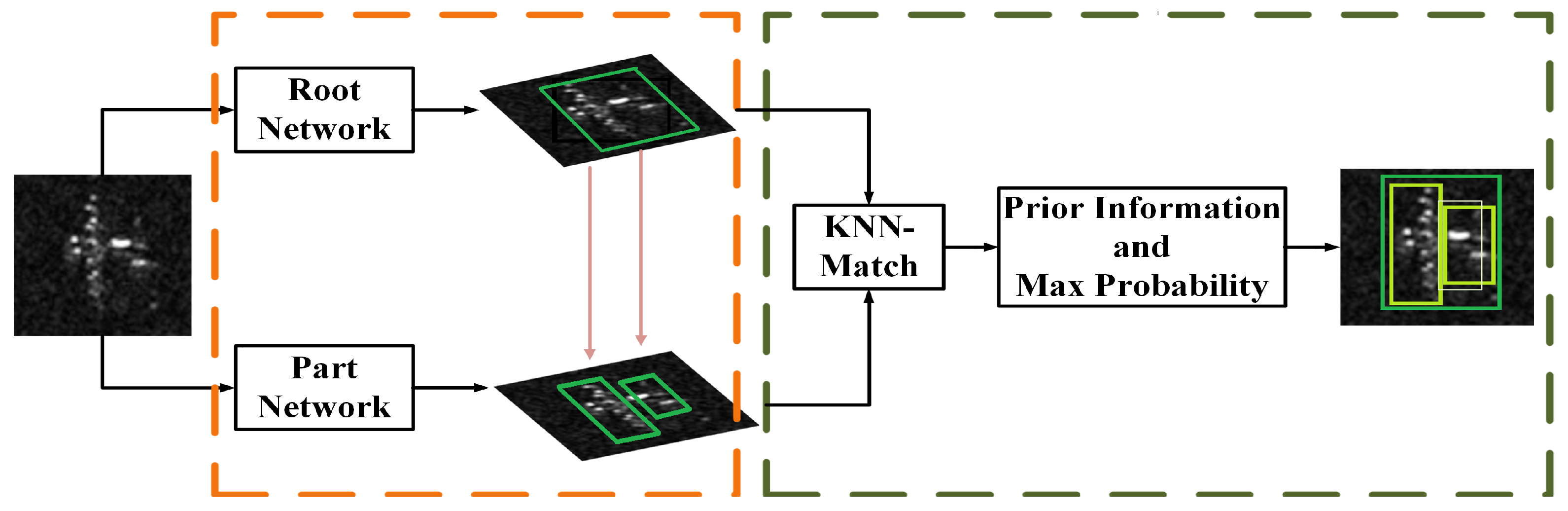
Inspired by the DPM method [8], objects of the same class always have similar parts. Focusing on airplane detection, each aircraft has a head, two wings and a tail. Due to different postures, the airplane components may have slightly different arrangement. However, the component relationship can still serve as priori information to optimize the detection results. Based on this idea, a component-based multi-layer parallel network is designed for airplane detection in SAR imagery. The detection structure consists of three layers: the first layer is to locate the whole object; the second layer is responsible for components detection; and the third layer utilizes the prior information and maximum probability for constraint and optimization. The overall algorithm framework is shown in Figure 1.

First, the trained root network and component network are adopted to detect the overall airplane and its components, respectively. Then, in the constraint layer, K-Nearest Neighbor (KNN) method [19] is used to filter mismatch between the object and the components. Finally, according to the maximum probability principle, the component information and detection probability are combined to eliminate the wrongly detected targets.

3.2. Parallel Detection Network

3.2.1. Training of the Detection Network

In the proposed algorithm, the root network is to locate the overall target and the part network is responsible for component detection. Targeting at airplane detection, only two categories, airplane and background, are set up for root network training, avoiding the interference of other categories. An airplane in SAR imagery is quite small, composed of hundreds of pixels, which brings difficulties for feature extraction. For component detection, each airplane target is divided into two components: the head and the tail. The training of the root and the component networks is consistent with YOLO algorithm. To adapt to the characteristics of SAR imagery, labeled images are employed for transfer learning of the first 20 convolution layers. Considering that various aspect ratio exist, a new parameter ${\lambda }_{\mathrm{aspect}}$ is introduced into the original objective function, to distinguish it from the coordinate error. The optimization objective is still square sum error, but modified as follows:

$$\begin{array}{c}\mathrm{loss}={\lambda }_{\mathrm{coord}}\sum _{i=0}^{S^2}\sum _{j=0}^B{1}_{ij}^{obj}[{(x_i-{\widehat{x}}_i)}^2+{(y_i-{\widehat{y}}_i)}^2]\hfill \end{array}$$

(2)

$$\begin{array}{c}+{\lambda }_{\mathrm{aspect}}\sum _{i=0}^{S^2}\sum _{j=0}^B{1}_{ij}^{obj}[{(\sqrt{w_i}-\sqrt{{\widehat{w}}_i})}^2+{(\sqrt{h_i}-\sqrt{{\widehat{h}}_i})}^2]\hfill \end{array}$$

(3)

$$\begin{array}{c}+\sum _{i=0}^{S^2}\sum _{j=0}^B{1}_{ij}^{obj}{(C_i-\widehat{C}{}_i)}^2\hfill \end{array}$$

(4)

$$\begin{array}{c}+{\lambda }_{noobj}\sum _{i=0}^{S^2}\sum _{j=0}^B{1}_{ij}^{nobj}{(C_i-\widehat{C}{}_i)}^2\hfill \end{array}$$

(5)

$$\begin{array}{c}+\sum _{i=0}^{S^2}{1}_i^{obj}\sum _{c\in classes}{(p_i(c)-{\widehat{p}}_i(c))}^2\hfill \end{array}$$

(6)

where ${\lambda }_{\mathrm{aspect}}$ is the aspect ratio weight. ${\lambda }_{\mathrm{coord}}=5$, ${\lambda }_{\mathrm{aspect}}=3$ is set during the root network training and ${\lambda }_{\mathrm{aspect}}=4$ when training the part network. Since aspect ratio of different components vary largely, to accurately detect the components, the suppression of the aspect ratio error should be appropriately increased.

3.2.2. Preliminary Detection

In preliminary detection, the bounding boxes of the whole airplane and each component are detected by the parallel network. The detection flow of the root and the part network are quite similar with that of YOLO algorithm. First, the image to be detected is scaled and divided into $7\times 7$ grids, and each grid is predicted to obtain the category score, confidence level and coordinates of the bounding boxes. Then, according to the output, the capture probability and coordinate information are computed and converted to the constraint layer. To facilitate the following optimization, the confidence level and category probability are utilized for calculating the capture probability, indicating the reliability of each bounding box. The formula of the capture probability is defined as follows:

$$P=\sqrt{P_{\mathrm{conf}}·P_{\mathrm{class}}}$$

(7)

where $P_{\mathrm{conf}}$ represents the confidence level and $P_{\mathrm{class}}$ denotes the category probability. In this way, the capture probability reflects the credibility of the bounding box and the class probability.

3.3. Discriminative Constraint Based on Priori Information and Maximum Probability

The second part of the framework is a constraint layer, in which the prior information and the maximum probability are combined to optimize the preliminary detection results. Elaborately, it can be divided into two steps: (1) KNN method is utilized to match the detected target box and the corresponding components;and (2) with the maximum probability as the priority criterion, the component information is adopted to constrain the detection results.

3.3.1. KNN Match

After the root network and the part network, all the possible bounding boxes of the targets and the components are obtained, but they do not have a clear correspondence. Therefore, a corresponding relationship between the root target and the components should be established, for subsequent discriminant constraint. The nearest two components are searched for each root target by the KNN method, so that the components and the target are linked accordingly.

In KNN algorithm, for a point set X, the nearest K points from each point are searched, according to a certain distance formula. The commonly used distance functions are shown in

Table 1. Distance calculation functions.

Strategies	Name	Calculation Formula
K-d Tree Search	Euclidean distance	$d_{st}^2=(x_s-y_t)(x_s-y_t{)}^{\prime }$
	Minkowski distance	$d_{st}=\sqrt[p]{{\displaystyle \sum _{j=1}^n}{\left|x_{sj}-y_{tj}\right|}^p}$
	Manhattan distance	$d_{st}={\displaystyle \sum _{j=1}^n}\left|x_{sj}-y_{tj}\right|$
	Chebyshev distance	$d_{st}={max}_j\left\{\left|x_{sj}-y_{tj}\right|\right\}$
	Correlation distance	$d_{st}=1-\frac{\left(x_s-{\overline{x}}_s\right)(y_t-{\overline{y}}_t{)}^{\prime }}{\sqrt{\left(x_s-{\overline{x}}_s\right)(x_s-{\overline{x}}_s{)}^{\prime }}\sqrt{\left(y_s-{\overline{y}}_s\right)(y_t-{\overline{y}}_t{)}^{\prime }}}$
Exhaustive Search	Standardized Euclidean distance	$d_{st}^2=(x_s-y_t)V^{-1}(x_s-y_t{)}^{\prime }$
	Mahalanobis distance	$d_{st}^2=(x_s-y_t)C^{-1}(x_s-y_t{)}^{\prime }$
	Angle cosine distance	$d_{st}=\left(1-\frac{x_s{y^{\prime }}_t}{\sqrt{(x_s{x^{\prime }}_s)(y_t{y^{\prime }}_t)}}\right)$
	Hamming distance	$d_{st}=\left(\#(x_{sj}\ne y_{tj})/n\right)$
	Jaccard distance	$d_{st}=\frac{\#[(x_{sj}\ne y_{tj})\cap (x_{sj}\ne 0)\cup (y_{tj}\ne 0)]}{\#[(x_{sj}\ne 0)\cup (y_{tj}\ne 0)]}$

. When sparse points to be searched are more than 20, the exhaustive search strategy [20] and Hamming distance [21] are employed. Oppositely, if non-sparse points do not exceed 20, K-d tree search strategy [22], Euclidean distance [23], and Manhattan distance [24] should be considered.

Actually, the formulas can be divided into distance metric and similarity measurement. Longer distances mean greater differences between individuals. Oppositely, the smaller is the similarity measure, the bigger is the difference between the points.

Euclidean distance measures the absolute distance between points, thus all dimensions should be in the same scale. Minkowski distance is a general expression for multiple distance measurements. In Table 1, when variable $p=1$ or tends to infinity, Manhattan distance and Chebyshev distance are obtained, respectively. Magnitude of different features has a large influence on Euclidean distance; therefore, for standardized Euclidean distance and Mahalanobis distance, each component is standardized.

Considering that similarity metric is not sensitive to magnitude, correlation distance is adopted to determine similarity between different variables. Cosine similarity is measured by the cosine value of the two vectors. Compared with distance metric, it focuses more on difference between vector direction rather than in length. Hamming distance is defined as the minimum number of substitutions to turn one into the other. In Jaccard distance, the proportion of different elements in the total is employed to measure the similarity of the two sets.

Distance measurement embodies the absolute difference of numerical characteristics between individuals, suitable for difference analysis of dimension values. Similarity concentrates more on direction and is insensitive to absolute values. Considering that there are not many points and absolute distance is important in our work, Euclidean distance is adopted in the KNN method. The basic search process is as follows:

a.

According to the target set, divide the search points into N regions.

b.

For the $i_{th}$ point in region I, search the k points that are closest to the target point in corresponding region I.

c.

For the distance of the kth point obtained in last step, find the region with the same distance.

d.

In the region that has been found, find the closer point.

3.3.2. Discriminative Constraint

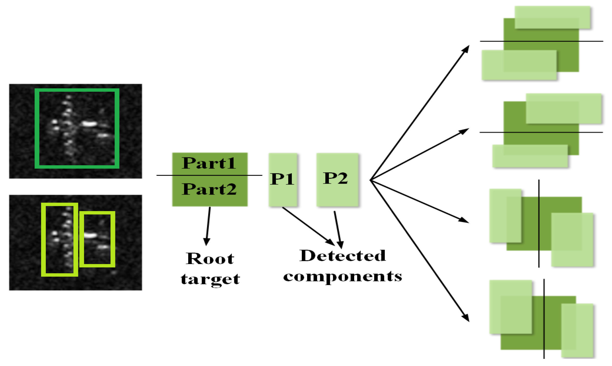
KNN algorithm finds the corresponding components for each root target; it is necessary to filter out the wrong detection results through the discriminative constraint. Actually, the airplane and its components are distributed in a certain rule, not arbitrarily arranged. The component distribution on the root airplane can be divided into several cases, as shown in Figure 2.

Assuming that the two components (the airplane head and the tail) are called P1 and P2, they can be presented as up–down or left–right, four conditions in total. When conducting the discriminative constraint, it is predefined that the root target is divided into two parts, accounting for $35\%$ and $65\%$ of the entire plane, respectively. The components P1 and P2 must overlap with either part more than $60\%$, and P1, P2 cannot be distributed on the same side, conforming to one of the above four cases. Once the conditions are met, the two components are assigned to the corresponding root target and can no longer be used by other targets. The overlap rate is calculated as follows:

$$overlap=\frac{area(part)\cap area(component)}{area(part)}$$

(8)

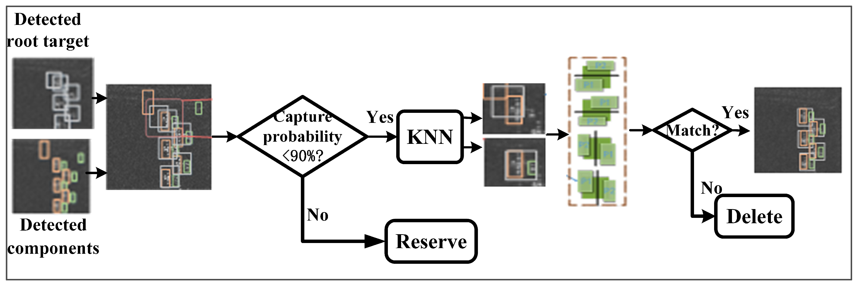
In this way, the root target can correctly match the components, thus most wrong detections are filtered out. However, if the components are missed, the correctly detected root target will have no matching components, increasing the missing detection rate. In response to this problem, the maximum probability criterion is introduced. When the capture probability of the root target is high enough, it can still be regarded as correct detection, even with no matching components. The overall discriminative constraining process is as follows and shown in Figure 3:

a.

If the capture probability of the root target is more than $90\%$, reserve the root target directly.

b.

For root targets with capture probability below $90\%$, calculate the overlap rate of the component with the root target. If no matching components are found, filter the root target.

c.

If both the overlap rates between component $P1$ and $P2$, and the root target are over $60\%$, estimate the component distribution.

d.

If the distribution of the two components does not belong to the four cases above, filter the corresponding root target, otherwise retain it as the final result.

With the strategies above adopted, the maximum probability can effectively reduce the error rate caused by miss-detection of the components.

3.4. Flow Chart of the Proposed Algorithm

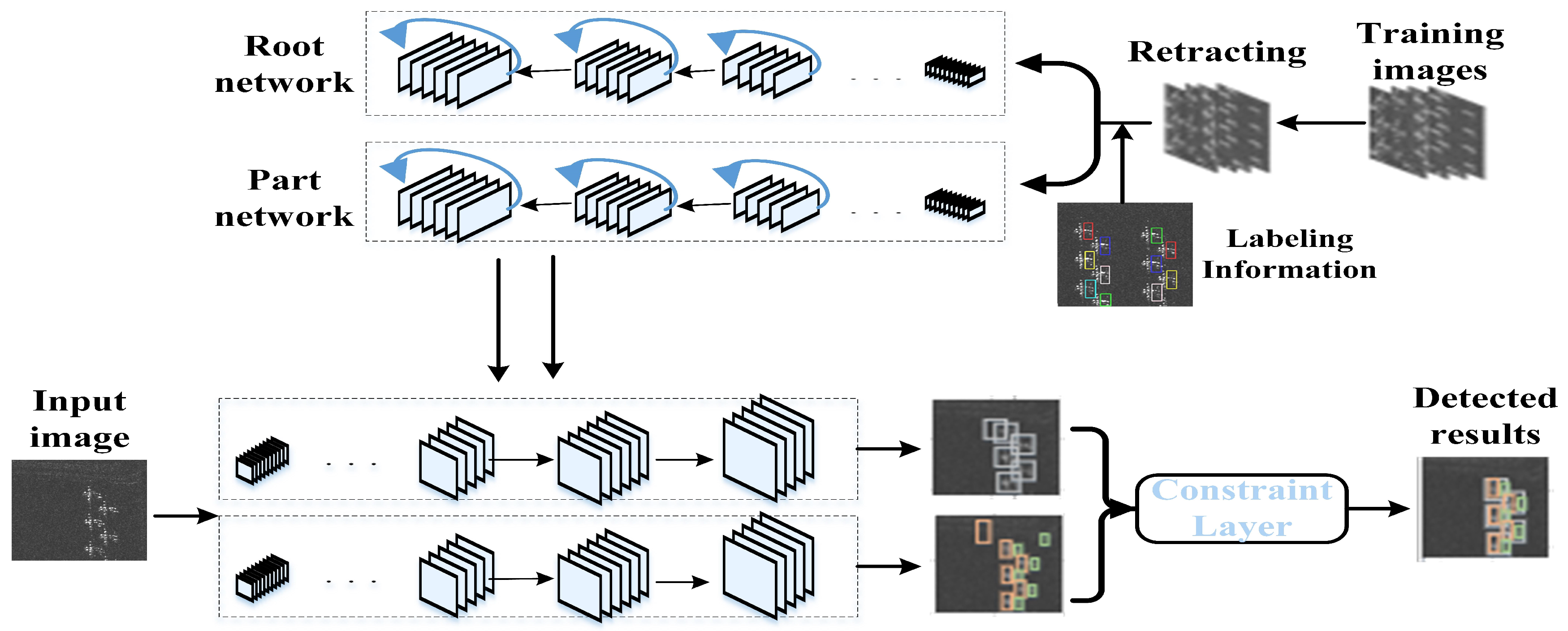
The overall framework of the proposed network is shown in Figure 4. Actually, it consists of two parts: network training and testing. First, for the training set, each airplane is labeled with one overall bounding box and two components (a head and a tail). Then, the labeled training images are utilized to train the root network and the part network. In the testing stage, the images to be detected are input to the network, and the root target and the components are detected, respectively. Finally, the preliminary detection results are input to the discriminative constraint layer, as shown in Figure 3, to obtain the optimized results.

4. Experiment

4.1. Experimental Data and Setting

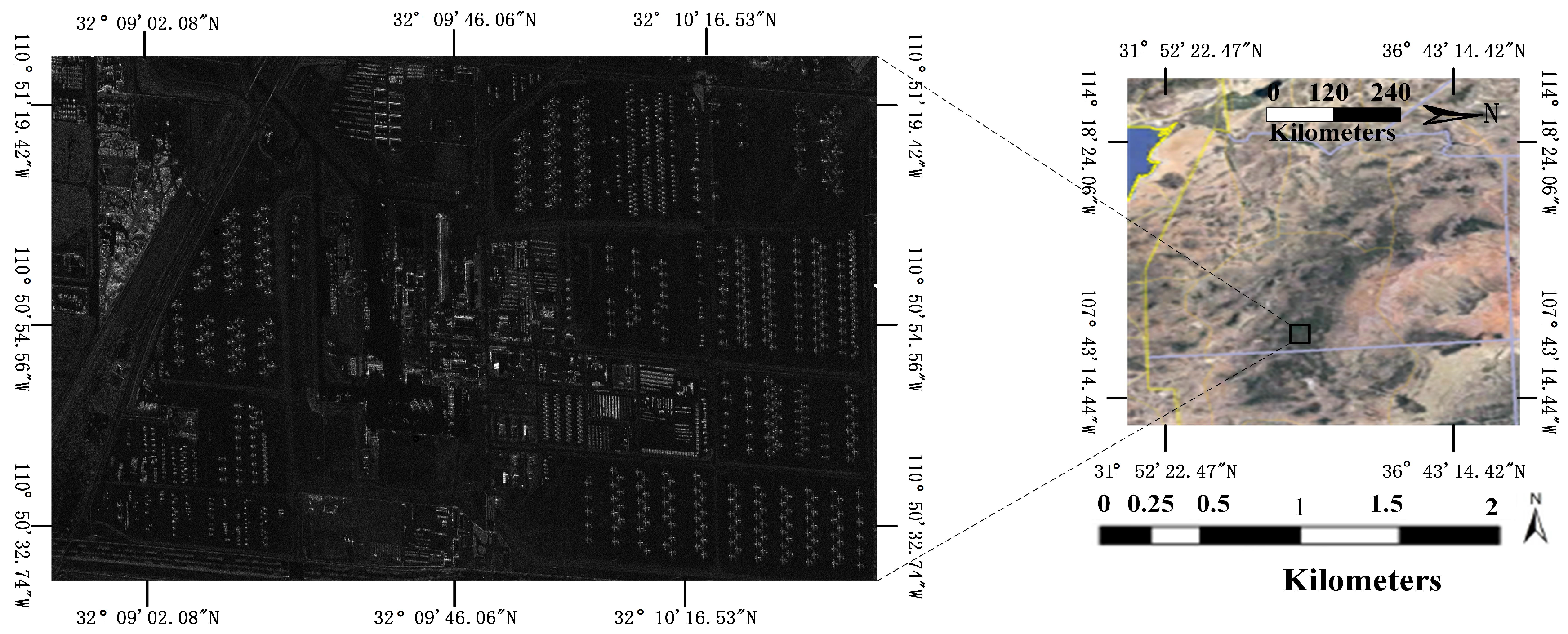
TerraSAR-X data obtained from Mount Davies Air Force Base, Arizona were adopted in this experiment. The Pauli SAR imagery has a resolution of 2 m and the image size is 11,296 × 6248 pixels. To accurately label the aircraft targets, optical image from Google Earth (2010) was utilized for corresponding reference. The SAR imagery and the optical image are shown in Figure 5 for contrast. There are more than 820 airplanes in the whole image, which is sliced into 120 figures. The training set has 110 pictures, containing 703 airplanes and the rest are for testing. In this paper, an airplane is divided into two components: a head and a tail. As a supervised algorithm, each airplane target is labeled with a global box and two bounding component boxes.

In this paper, the proposed method is the component-based multi-layer parallel network and the classical detection algorithm (CFAR) method serves as a benchmark approach. Based on DPM [8], an Adaptive Component Selection-Based Discriminative Model (ACSDM) [25] is another comparative method. Note that experiments about CFAR and ACSDM methods have been conducted, as shown in Reference [25]. To properly compare the three approaches above, the same SAR data and evaluation criterion were adopted in this work. For clear illustration, the same assess indexes are presented as follows:

$$P=\frac{N_{cd}}{N_d},$$

(9)

$$P_{fa}=\frac{N_{fd}}{N_d},$$

(10)

$$R=\frac{N_{cd}}{N_t}.$$

(11)

In Equation (9), $N_d$ is the number of all detected objects, and $N_{cd}$ and $N_{fd}$ represent the number of correctly detected aircrafts and objects that are falsely detected as aircraft, respectively. Therefore, $N_d=N_{cd}+N_{fd}$. $N_t$ indicates the number of total aircrafts, including the correctly detected aircrafts and the missing number; in the following experiments, $N_t=117$. These indexes are counted in each image individually, then, the overall measurement indexes are added up and computed.

4.2. Experimental Results and Analysis

Tables 1 and 3 in Reference [25], and

Table 2. Detection results of the proposed algorithm.

Region	Labeled Image	Root Detection Results	Final Detection Results
Region 1
Region 2
Region 3
Region 4
Region 5
Region 6
Region 7
Region 8
Region 9
Region 10

present the airplane detection results of CFAR, ACSDM and the proposed network, respectively.

In the CFAR results, owing to sparsity and diversity, airplane targets consisting of scattering points cannot be completely detected. Besides, some high-brightness adjacent points belonging to one aircraft are also detected as multiple targets by mistake. Therefore, CFAR method has a relatively high false alarm rate and the performance is not effective enough. As for the ACSDM model, it achieves better detection results than CFAR method. As shown in Table 3 in Reference [25], most targets are accurately located with proper component positions, demonstrating that component information is contributing for object detection. However, some unknown objects are wrongly detected as airplanes while some other airplane targets are not correctly detected. In Table 2, the proposed network presents the best performance among the three detection methods. It is clear that all airplanes in the testing images are correctly detected. For each airplane target, the blue bounding box means the root location, yellow box and green box indicate the detected airplane head and tail, respectively. Besides, there is no presence that multiple airplanes are detected as one target.

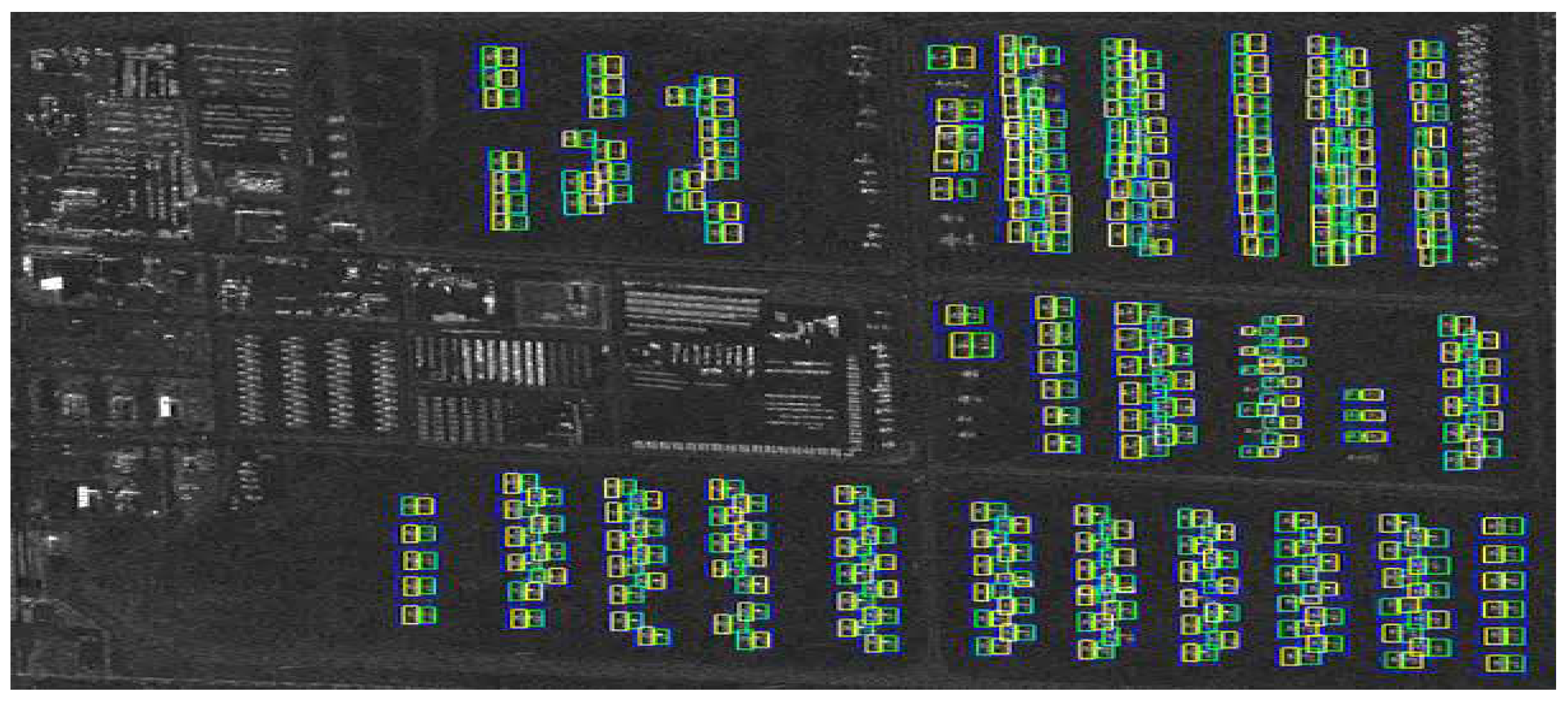
On the whole image, Figure 6 shows the overall detection results by the proposed method. There are conventional airplanes and micro-airplanes in the imagery. Labeling for the latter is difficult, therefore, micro-airplanes are excluded in the experiments. Since acquisition of SAR imagery is quite demanding, the dataset for experiments is usually a bit small, compared with optical images. In the overall detection results, eight airplanes are missed but there were no wrong detections.

To give more convincing evidence, the detection number of different methods are shown in Tables 2 and 4 in Reference [25], and

Table 3. Detection number of the proposed algorithm.

Region	Two stages	Correctly Detected Number ${\mathit{N}}_{\mathit{cd}}$	Missing Number	Wrongly Detected Number ${\mathit{N}}_{\mathit{fd}}$
Region 1	Root detection	12	0	0
	Final detection	12	0	0
Region 2	Root detection	20	0	3
	Final detection	20	0	0
Region 3	Root detection	8	0	0
	Final detection	8	0	0
Region 4	Root detection	5	0	1
	Final detection	5	0	0
Region 5	Root detection	11	0	1
	Total detection	11	0	0
Region 6	Root detection	17	0	1
	Final detection	17	0	0
Region 7	Root detection	8	0	0
	Final detection	8	0	0
Region 8	Root detection	8	0	1
	Final detection	8	0	0
Region 9	Root detection	15	0	1
	Final detection	15	0	0
Region 10	Root detection	13	0	2
	Final detection	13	0	1
Total	Root detection	117	0	10
	Final detection	117	0	1

. There are totally 117 airplanes in the 10 testing images. In the detection results of CFAR method, the missing number is 8 and the wrongly detected number is 40, resulting in the highest false alarm rate. The missing number of ACSDM model is similar to that of CFAR detection results. However, the wrongly detected number is largely reduced to one tenth. Besides, there is no case that scattering points belong to one airplane are detected as multiple objects. It proves that utilizing component information is effective in dealing with sparsity in SAR imagery. However, the problem caused by diversity still exists in the detection results of the ACSDM model. In the proposed network, depth feature and component information are adopted to cope with sparsity and diversity for airplane detection in SAR imagery. As shown in Table 3, all airplanes in the testing images are correctly detected. Compared with CFAR method and the ACSDM model, the proposed approach has the highest detection accuracy and the lowest false alarm rate. Even though 10 objects are falsely detected as airplanes in the root detection, there is one wrong detection left in final detection (after the constraint layer). It demonstrates that the constraint layer does effectively optimize the detection performance.

For better evaluation, the overall measuring indexes and time consumption of different methods are presented in

Table 4. Measuring indexes of different methods.

Methods	Accuracy P	False Alarm Rate ${\mathit{P}}_{\mathit{fa}}$	Recall Rate R	Training Time	Detection Time
CFAR Algorithm	0.732	0.268	0.932	/	20 s
ACSDM Model	0.964	0.036	0.915	5 h	7 s
The Proposed Appro.	0.992	0.008	1	22 h	0.9 s

. The recall rate R of ACSDM model is lower than that of CFAR method, but the former has a higher accuracy and a lower false alarm rate. In general, the proposed network exhibits the best performance with the highest accuracy and recall rate and the lowest false alarm rate. As for time consumption, the proposed approach is network-based and has the longest training time. As a supervised method, the ACSDM model also requires 5 h for training. The traditional CFAR-based method needs no training. However, the detection time shows the opposite pattern. The proposed algorithm has obvious advantage and only costs 0.9 s for detection, followed by the ACSDM model, while detection time of CFAR method is the longest.

4.3. Discussion

To further improve the accuracy and apply the proposed method in practical situations, the following aspects are considered. Because of the regular array, it is suspected that the network somehow learns the periodicity.

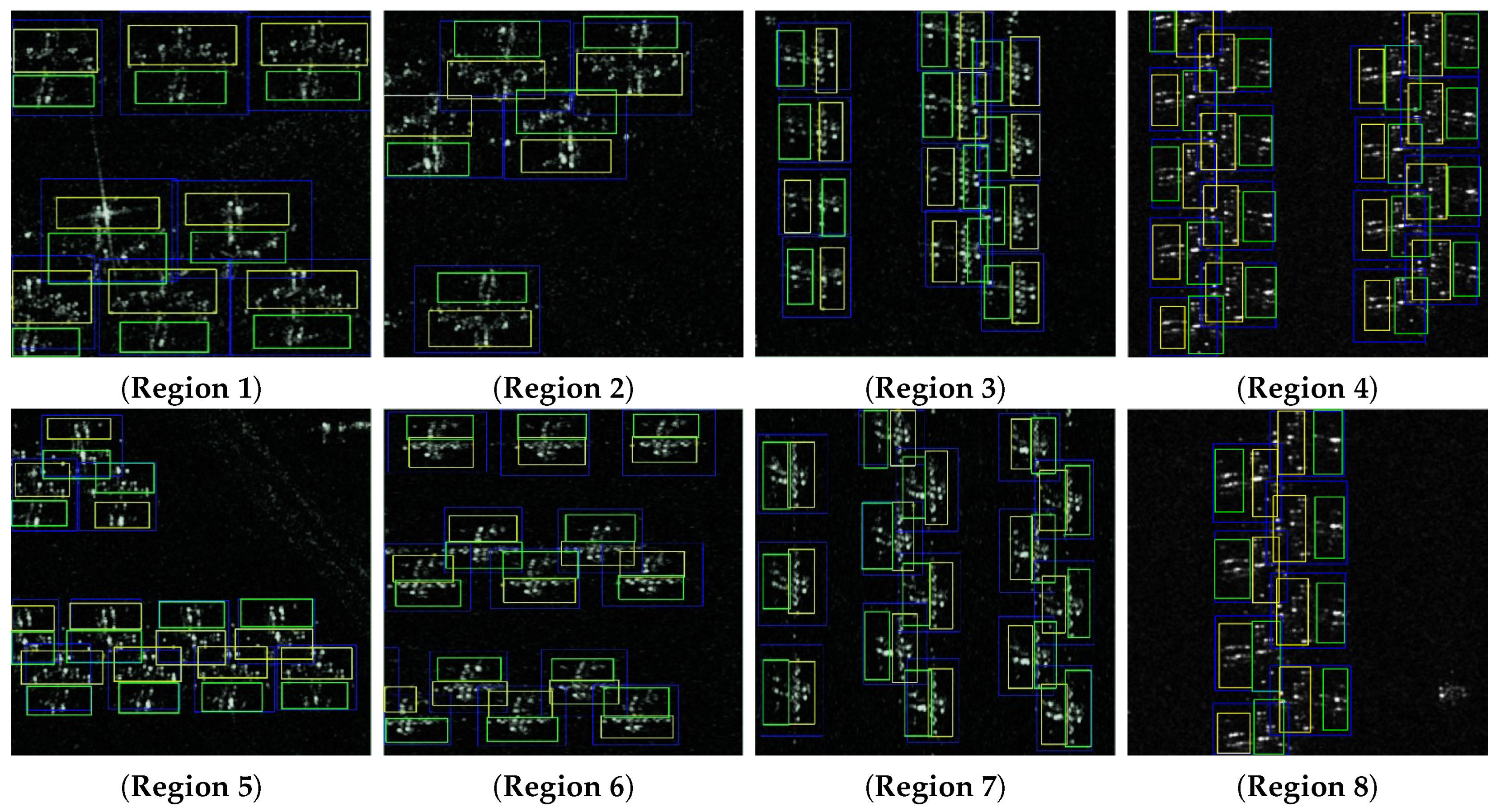
In our work, the arrangement of the airplanes is quite regular, with almost all airplane heads towards left. The original network to test images in which the objects have similar orientations might not be convincing enough. Since we do not have SAR images where the airplanes are parked in disorder, the testing images are rotated with ${90}^{\circ }$, 180${}^{\circ }$ and −90${}^{\circ }$ to get airplanes with different orientations. Synchronously, the labeled samples are also rotated to obtain the newly trained network and the corresponding detection results are shown in Figure 7:

From the detection results above, it is clear that all airplanes are correctly detected. It is demonstrated that the network learns the characteristics rather than periodicity to detect the objects correctly. Besides, from Region 4, we can see that aircrafts in the two columns are actually arranged face-to-face. However, the original network can still detect all aircrafts, which to some extent, refutes the proposition that the “network learns periodicity”.

5. Conclusions

Aiming at airplane detection in SAR images, depth characteristics and component structure are adopted to cope with diversity and sparsity, respectively. Drawing on YOLO algorithm, this paper proposes a component-based multi-layer parallel network for detecting aircrafts. In the proposed approach, the overall target and the components are preliminarily located by the parallel network. In the following constraint layer, KNN method is utilized to match the detected airplane and the corresponding components. Then, with maximum probability as criterion, prior structure information is employed to optimize the detection results. In this paper, experiments about the proposed approach is carried out on TerraSAR data, with CFAR method and ACSDM model for comparison. In the testing images, each airplane is accurately located by the presented network. There are 10 wrong detections in preliminary detection but only one left in final results, proving that the constraint layer is effective in dealing with sparsity in SAR imagery. Compared with CFAR method and the ACSDM model, depth feature in the proposed network is characterized by continuous iterative training and has a stronger adaptability than handmade HOG features. Therefore, missing detection of the presented network is much less. Future work will focus on merging the root network with the component network, to obtain bounding boxes of the root and the components directly. This method saves much computation and improves the training speed.

References

- Van Zyl, J.; Kim, Y. Synthetic Aperture Radar Polarimetry; John Wiley & Sons, Inc.: Hoboken, NJ, USA, 2011. [Google Scholar]
- He, C.; Li, S.; Liao, Z.; Liao, M. Texture classification of PolSAR data based on sparse coding of wavelet polarization textons. IEEE Trans. Geosci. Remote Sens. 2013, 51, 4576–4590. [Google Scholar] [CrossRef]
- Finn, H.M. Adaptive detection mode with threshold control as a function of spatially sampled clutter-level estimates. RCA Rev. 1968, 29, 414–464. [Google Scholar]
- Hansen, V.G. Constant false alarm rate processing in search radars. Radar Present Future 1973, 105, 325–332. [Google Scholar]
- Trunk, G.V. Range resolution of targets using automatic detectors. IEEE Trans. Aerosp. Electron. Syst. 1978, AES-14, 750–755. [Google Scholar] [CrossRef]
- Kuttikkad, S.; Chellappa, R. Non-Gaussian CFAR techniques for target detection in high resolution SAR images. In Proceedings of the 1st International Conference on Image Processing, Austin, TX, USA, 13–16 November 1994; Volume 1, pp. 910–914. [Google Scholar]
- Tello, M.; Lopez-Martinez, C.; Mallorqui, J.J. A novel algorithm for ship detection in SAR imagery based on the wavelet transform. IEEE Geosci. Remote Sens. Lett. 2005, 2, 201–205. [Google Scholar] [CrossRef]
- Felzenszwalb, P.F.; Girshick, R.B.; Mcallester, D.; Ramanan, D. Object detection with discriminatively trained part-based models. IEEE Trans. Pattern Anal. Mach. Intell. 2010, 32, 1627–1645. [Google Scholar] [CrossRef] [PubMed]
- Tan, Y.; Li, Q.; Li, Y.; Tian, J. Aircraft Detection in High-Resolution SAR Images Based on a Gradient Textural Saliency Map. Sensors 2015, 15, 23071–23094. [Google Scholar] [CrossRef] [PubMed] [Green Version]
- Dou, F.; Diao, W.; Sun, X.; Wang, S.; Fu, K.; Xu, G. Aircraft recognition in high resolution SAR images using saliency map and scattering structure features. In Proceedings of the Geoscience and Remote Sensing Symposium (IGARSS), Beijing, China, 10–15 July 2016; pp. 1575–1578. [Google Scholar]
- Deng, L.; Yu, D. Deep Learning: Methods and Applications. Found. Trends Signal Process. 2014, 7, 197–387. [Google Scholar] [CrossRef] [Green Version]
- Girshick, R.; Donahue, J.; Darrell, T.; Malik, J. Rich feature hierarchies for accurate object detection and semantic segmentation. In Proceedings of the IEEE Conference on Computer Vision and Pattern Recognition, Columbus, OH, USA, 23–28 June 2014; pp. 580–587. [Google Scholar]
- Ross, G. Fast R-CNN. In Proceedings of the 2015 IEEE International Conference on Computer Vision, Washington, DC, USA, 7–13 December 2015; pp. 1440–1448. [Google Scholar]
- Ren, S.; He, K.; Girshick, R.; Sun, J. Faster R-CNN: Towards real-time object detection with region proposal networks. IEEE Trans. Pattern Anal. Mach. Intell. 2015, 39, 1137–1149. [Google Scholar] [CrossRef] [PubMed]
- Joseph, R.; Divvala, S.; Girshick, R.; Farhadi, A. You only look once: Unified, real-time object detection. In Proceedings of the IEEE Conference on Computer Vision and Pattern Recognition (CVPR), Las Vegas, NV, USA, 27–30 June 2016; pp. 779–788. [Google Scholar]
- He, C.; Zhuo, T.; Ou, D.; Liu, M.; Liao, M. Nonlinear compressed sensing-based LDA topic model for polarimetric SAR image classification. IEEE J. Sel. Top. Appl. Earth Obs. Remote Sens. 2014, 7, 972–982. [Google Scholar] [CrossRef]
- Minaee, S.; Abdolrashidiy, A.; Wang, Y. An experimental study of deep convolutional features for iris recognition. In Proceedings of the 2016 IEEE Signal Processing in Medicine and Biology Symposium (SPMB), Philadelphia, PA, USA, 3 December 2016; pp. 1–6. [Google Scholar]
- Russakovsky, O.; Deng, J.; Su, H.; Krause, J.; Satheesh, S.; Ma, S.; Huang, Z.; Karpathy, A.; Khosla, A.; Khosla, M.; et al. ImageNet Large Scale Visual Recognition Challenge. Int. J. Comput. Vis. 2015, 115, 211–252. [Google Scholar] [CrossRef] [Green Version]
- Parvin, H.; Alizadeh, H.; Minati, B. A Modification on K-Nearest Neighbor Classifier. Glob. J. Comput. Sci. Technol. 2010, 10, 37–41. [Google Scholar]
- Amal, M.A.; Riadh, B.A.A. Survey of Nearest Neighbor Condensing Techniques. Int. J. Adv. Comput. Sci. Appl. 2011, 2, 59–64. [Google Scholar] [CrossRef]
- Vijay, R.; Mahajan, P.; Kandwal, R. Hamming Distance based Clustering Algorithm. Int. J. Inf. Retr. Res. 2012, 2, 11–20. [Google Scholar] [CrossRef]
- Mahadi, S.; Kokate, S. A Fast nearest Neighbor Search Using K-D Tree and Inverted Files. Int. J. Adv. Res. Comput. Sci. Manag. Stud. 2016, 4, 362–367. [Google Scholar]
- Xia, S.; Xiong, Z.; Luo, Y.; Xu, W.; Zhang, G. Effectiveness of the Euclidean distance in high dimensional spaces. Opt. Int. J. Light Electron Opt. 2015, 126, 5614–5619. [Google Scholar] [CrossRef]
- Kaur, D. A Comparative Study of Various Distance Measures for Software fault prediction. Int. J. Comput. Trends Technol. 2014, 17, 117–120. [Google Scholar] [CrossRef] [Green Version]
- Chu, H.; Mingxia, T.; Dehui, X.; Feng, T.; Mingsheng, L. Adaptive Component Selection-Based Discriminative Model for Object Detection in High-Resolution SAR Imagery. ISPRS Int. J. Geo-Inf. 2018, 7, 72. [Google Scholar] [Green Version]
Figure 1.
Framework of the component-based multi-layer parallel network for airplane detection.
Figure 2.
Four possible component locations on the root target.
Figure 3.
Discriminative constraint layer.
Figure 4.
Algorithm flow chart.
Figure 5.
TerraSAR-X data adopted in our work.
Figure 6.
Detection result of the whole imagery.
Figure 7.
Detection results of the newly trained network.