A Novel Object-Based Supervised Classification Method with Active Learning and Random Forest for PolSAR Imagery


1
State Key Laboratory of Information Engineering in Surveying, Mapping and Remote Sensing, Wuhan University, Wuhan 430079, China
2
School of Electrical and Computer Engineering, Purdue University, West Lafayette, IN 47907, USA
*
Author to whom correspondence should be addressed.
Remote Sens. 2018, 10(7), 1092; https://doi.org/10.3390/rs10071092
Submission received: 21 May 2018
/
Revised: 24 June 2018
/
Accepted: 3 July 2018
/
Published: 9 July 2018
(This article belongs to the Special Issue Classification and Feature Extraction for Remote Sensing Image Analysis)
Abstract
:Most of the traditional supervised classification methods using full-polarimetric synthetic aperture radar (PolSAR) imagery are dependent on sufficient training samples, whereas the results of pixel-based supervised classification methods show a high false alarm rate due to the influence of speckle noise. In this paper, to solve these problems, an object-based supervised classification method with an active learning (AL) method and random forest (RF) classifier is presented, which can enhance the classification performance for PolSAR imagery. The first step of the proposed method is used to reduce the influence of speckle noise through the generalized statistical region merging (GSRM) algorithm. A reliable training set is then selected from the different polarimetric features of the PolSAR imagery by the AL method. Finally, the RF classifier is applied to identify the different types of land cover in the three PolSAR images acquired by different sensors. The experimental results demonstrate that the proposed method can not only better suppress the influence of speckle noise, but can also significantly improve the overall accuracy and Kappa coefficient of the classification results, when compared with the traditional supervised classification methods.
1. Introduction
Land-cover classification of remote sensing imagery is becoming more and more important for local and regional planning [1,2], environmental impact assessment [3,4], agriculture monitoring [5], etc. Meanwhile, classification methods using optical remote sensing images have been extensively developed in recent decades because of the widespread accessibility of optical imagery. However, optical remote sensing images are subject to the influence of weather and illumination [6]. Fortunately, PolSAR data can not only overcome the disadvantages of optical remote sensing images, but can also allow improved object interpretation through making full use of the polarimetric information of PolSAR imagery [7].
Several supervised classification methods for PolSAR imagery have been developed, such as the Wishart supervised classifier [1], convolutional neural networks (CNN)-based classifier [8], the support vector machine (SVM) classifier [9], and the random forest (RF) classifier [10], and they have shown good performances when the training samples are sufficient. However, the collection of training sample sets is complicated and expensive; moreover, the process of traditional classification is time-consuming due to the redundant training samples. Fortunately, the active learning (AL) method [11,12] has been developed in recent years, which can obtain a better classification performance than the traditional supervised classification methods when the training samples are limited. Although numerous methods using AL have been successfully applied to hyperspectral remote sensing images [11,12,13], the AL method has rarely been applied to full-polarimetric SAR images, due to the influence of the complex imaging mechanism, such as foreshortening, shadow, and overlay. At the same time, PolSAR images are subject to the influence of inherent speckle noise and still have finely divided spots despite speckle filtering, so the results of the traditional pixel-based supervised classification methods show a high false alarm rate. Therefore, supervised classification using full-polarimetric SAR data remains a challenge. In this regard, it is necessary to design a supervised classification method for PolSAR imagery that uses as few labeled samples as possible to obtain better precision.
In this paper, focusing on the aforementioned problems of the traditional supervised classification methods when using PolSAR imagery, we propose an object-based classification method named GSRM_MBT_RF to enhance the classification performance. The proposed method should not be regarded as a combination of many different methods, but rather as a fully unified algorithm with different steps. The GSRM method is used to reduce the impact of inherent speckle noise; the AL algorithm is applied to select reliable training samples from the different polarimetric features of the PolSAR imagery; and the RF classifier is used as the classifier to identify the different types of land cover in the PolSAR images.
The rest of this paper is organized as follows. The proposed object-based supervised classification method with AL and RF is described in Section 2. Section 3 details the results of the proposed approach on different PolSAR images from different sensors. Section 4 discusses the results of the case study. Finally, our conclusions are drawn in Section 5.
2. Materials and Methods
In this paper, a novel object-based supervised classification method which integrates the advantages of three different algorithms (the GSRM algorithm, the AL method, and the RF classifier) is proposed for the classification of PolSAR imagery. The procedure of the proposed method is introduced in this section.
2.1. Polarimetric Feature Extraction
Generally speaking, PolSAR imagery includes the backscattering coefficients of the four polarimetric channels (HH/HV/VH/VV) [1]. For the orthogonal polarization basis, the scattering information of ground objects can be represented by the following Sinclair matrix S [14]:
The different elements in matrix S represent the backscattering coefficients of the different polarimetric channels. For multi-look conditions, the covariance matrix C of the PolSAR imagery obeys a complex Wishart distribution under the reciprocity hypothesis in mono-station case.
To better achieve object interpretation, it is necessary to acquire the parameters of the polarimetric features based on a physical scattering mechanism [15]. The backscattering coefficients (, and ) are the basic polarimetric features of PolSAR imagery. Meanwhile, the copolarized correlation coefficient () can represent the attenuation and randomness of different natural objects.
The theorems of polarimetric decomposition, which are related to the properties of different objects, can also be used to extract the different polarimetric features of PolSAR imagery. In recent years, several polarimetric decomposition methods have been developed and applied. In this study, we extracted the polarimetric features using different methods of polarimetric decomposition. A summary of the polarimetric parameters used in this study is shown in Table 1, including Cloude polarimetric decomposition [15], H/A/Alpha polarimetric decomposition [16], Freeman–Durden three-component decomposition [17], van Zyl decomposition [18], Yamaguchi decomposition [19], TSVM decomposition [20] and Arii decomposition [21]. The polarimetric features were extracted using the Polarimetric SAR Data Processing and Educational Tool (PolSARpro).
2.2. Generalized Statistical Region Merging (GSRM)
PolSAR imagery is usually subjected to the impact of inherent speckle noise, which leads to a poor performance for the traditional pixel-based supervised classification methods [22]. Fortunately, object-based classification algorithms have the potential to suppress the influence of speckle noise, and we can also use spatial feature information when using a supervised classification method [23]. Segmentation is one of the most important aspects of the object-based classification algorithms, and a number of algorithms based on segmentation of PolSAR imagery have been developed in recent years, such as the GSRM algorithm [24], the mean shift segmentation algorithm [25], and the normalized cut (Ncut) segmentation algorithm [26].
The GSRM algorithm has a number of advantages, such as rapid computation and the fact that it is independent of the data distribution, when compared with some of the traditional segmentation methods using PolSAR data [24]. Therefore, the GSRM algorithm has been widely applied in the segmentation of PolSAR imagery [27,28,29]. Two essential components are defined when using the GSRM algorithm: (1) the merging predicate, which is used to confirm whether adjacent regions are merged or not; and (2) the merging order, which is followed to test the merging of regions.
2.2.1. Merging Predicate
The merging predicate of the GSRM algorithm can be derived from the theory of probability [30]. If (R, R’) is a pair of adjacent areas of an observed PolSAR imagery I, for any δ (0 < δ ≤ 1), a corollary can be represented according to the Nock and Nielsen model [30]:
where Q is the maximum value of the PolSAR imagery, and is uncertain. stands for cardinal and is the expectation over all corresponding statistical pixels. Parameter B is set as 2 in this paper [24].
As a result, a merging predicate can be obtained as follows:
where
2.2.2. Merging Order
The merging order of the GSRM algorithm is not a stepwise optimization tactic, but is rather a pre-ordering strategy. Under the guidance of pre-ordering, the first step of the merging order calculates the gradient from the gradient function :
where and is a pair of adjacent pixels in the PolSAR imagery. The second step of the merging order sorts the order of in increasing order and merge regions of p and p’ represent.
2.3. Active Learning (AL)
Most of the supervised classification methods for PolSAR imagery are limited by the availability of effective training samples. Moreover, the process of classification is time-consuming due to the redundant information of training samples. To address these issues, the AL method has been introduced in recent years [13]. AL method can be used to better select a reliable training set from unlabeled data, and has been successfully applied in the supervised classification of optical imagery [31].
An AL algorithm is aimed at iteratively enlarging the training samples by human–machine interaction, and labels samples with the maximum information from a set of unlabeled features for each class [32]. The basic function of AL can be represented as follows [33]:
where component C represents the classifier used in the AL method; component L is a group of labeled training sets for each class; component Q stands for the query function, which is used to query the informative training samples; component U represents the unlabeled features of the PolSAR data; and component S stands for the unlabeled set to be labeled. The general process of AL is shown in Algorithm 1.
| Algorithm 1. The general process of AL. |
| Input: labeled sample set L, unlabeled sample set , the number of training sample sets 1. Initialize training sample set based on random selection from labeled sample set L 2. While size of training sample set do 3. Learn a model by classifier C according to training sample set 4. Select the most informative samples based on query function Q 5. Label the most informative samples from unlabeled sample set U 6. Update unlabeled sample set and new labeled sample set 7. 8. End while Output: the training sample set of the most informative samples |
The query function plays a key role in the AL method. Different schemes of sample selection have been developed in recent years, such as membership query synthesis, which includes stream-based selective sampling and pool-based selective sampling [32]. The pool-based query methods are some of the most popular methods, and they can make the best use of the posterior probabilities for each class [33]. Four different sampling schemes based on polarimetric and contextual information were implemented in this study: (1) random selection (RS), which selects the training samples from the unlabeled candidate pool using a random method; (2) a mutual information (MI)-based criterion; (3) the breaking ties (BT) algorithm; and (4) a modified breaking ties (MBT) scheme [11,13].
2.3.1. The Mutual Information (MI)-Based Criterion
The MI-based criterion [11] of AL method obtains the training samples by maximizing the mutual information between the classifier and class labels, which can select samples from the most complicated region. We suppose that stands for the MI between the classifier and the class labels, and a new feature vector is selected. The MI-based criterion of AL method can then be represented as follows:
where
where H is the Hessian matrix, and stands for the Hessian matrix after including the new polarimetric feature . H and can be represented as follows:
where represents the posterior probabilities of class labels, which we can obtain by Bayes’ theorem. Component stands for the input polarimetric feature. is an operation of the Kronecker product. We obtain the MI by combining Equations (8)–(10).
where K represents the number of categories.
2.3.2. Breaking Ties (BT) Algorithm
The BT algorithm [32] selects the training samples by minimizing the distance of the two most probable classes, and it can select samples from the boundary region between the two most probable classes. The BT algorithm for AL method can be represented as follows:
where stands for the most probable class for feature vector , which is the maximum of the posterior probabilities of class labels; and represents the second most probable class for feature vector , which can also be easily obtained by Bayes’ theorem [11,13].
2.3.3. The Modified Breaking Ties (MBT) Algorithm
Even though the MI-based criterion and BT algorithm can obtain better performances than RS, they do have some disadvantages: (1) the MI-based criterion focuses on the most complicated area, so it is prone to confused among different classes and less accurate; and (2) the BT algorithm focuses on the boundary area between the two most probable classes, so it is prone to having only one boundary. Fortunately, the MBT scheme was put forward, which can promote more diversity than the other two methods [13]. The goal of MBT scheme is to obtain the training samples by calculating the minimum probability between the largest classes in each individual class.
The MBT scheme includes two main steps: the first step of MBT is to select samples from the unlabeled pool according to the samples with the same maximum a posteriori (MAP) estimation; and the second step of MBT is used to iteratively select samples from the most complicated region according to the following Formula (13):
where stands for the most possibility of each class for feature vector .
2.4. The Procedure of the Proposed Method
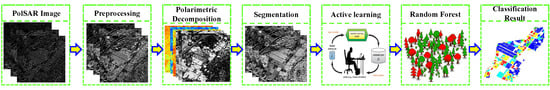
The basic processing procedure of the proposed method (as shown on Figure 1) consists of: (1) preprocessing of the PolSAR imagery; (2) polarimetric decomposition and feature extraction; (3) segmentation of PolSAR imagery, i.e., delineation of the land parcels using the GSRM algorithm; (4) selection of an effective training set; and (5) image classification.
In this proposed method, it is essential to preprocess the PolSAR imagery because of the complexity of the PolSAR imaging procedure and the characteristics of phase coherence processing. The preprocessing of PolSAR data includes: (1) radiation correction; and (2) filtering. In this study, the radiation correction was implemented using PolSARpro software and Next ESA SAR Toolbox (NEST) software. The Lee Sigma filter has the advantages of being able to retain better details and a reduced time cost when compared with other filter methods [7], so we chose the 7 × 7 Lee Sigma filter to suppress the speckle noise. The different polarimetric features were extracted using PolSARpro software, and the GSRM algorithm was used to reduce the impact of the inherent speckle noise in the next step. The AL algorithm was then applied to select reliable training samples from the different polarimetric features of the PolSAR imagery. Finally, the RF classifier was used as the classifier to identify the different types of land cover in the PolSAR images.
3. Experiments and Results
Three PolSAR image datasets were used for the evaluation of the proposed method and our method was implemented using MATLAB language. To evaluate the effectiveness of the proposed method, we compared the overall accuracy (OA) and Kappa coefficient (Kappa) of the experimental results with those of other classifiers that select data points either at random or via another related sample selection strategies.
3.1. Description of the Image Datasets
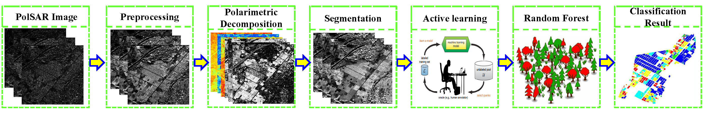
In the experiments, the first full-polarimetric SAR dataset used was obtained by the Airborne Synthetic Aperture Radar (AIRSAR) sensor. The imagery is L-band data acquired by NASA/JPL from Flevoland in the Netherlands in 1989. The PolSAR imagery size is 750 × 1024 pixels and the spatial resolution is 6.60 m × 12.10 m. The Pauli-RGB imagery is shown in Figure 2a and the ground truth is shown in Figure 2b. The land-cover types of this area are mainly crops, and 15 different land-cover categories are listed in Figure 2c.
The second full-polarimetric SAR dataset was acquired by the 38th Research Institute of the China Electronics Technology Group Corporation (CETC38) in 2012. This imagery is an Uninhabited Aerial Vehicle Synthetic Aperture Radar (UAVSAR) imagery (X-band) of an area near the city of Lingshui in China. The Pauli-RGB image is shown in Figure 2d. The PolSAR image size is 2220 × 2333 pixels and the spatial resolution is 0.5 m × 0.5 m. The ground truth of the PolSAR image is shown in Figure 2e, which was established by on-the-spot field investigation. Five different growth stages of paddy fields are identified in Figure 2f.
The third full-polarimetric SAR dataset was acquired by the Radarsat-2 on 7 December 2011. This imagery is a C-band of an area near the city of Wuhan, in China. The Pauli-RGB image is shown in Figure 2g. The PolSAR image size is 1200 × 1000 pixels and the spatial resolution is 8.0 m × 8.0 m. The ground truth of the PolSAR image is shown in Figure 2h, which was obtained by visual interpretation of the optical imagery corresponding to the time of Radarsat-2 imagery. Four different land-cover categories are listed in Figure 2i.
3.2. Experiments and Results
3.2.1. Experiments with AIRSAR Image
In this set of experiments, 15 land-cover categories were considered for the classification. Polarimetric decomposition was implemented to extract the polarimetric parameters from the AIRSAR data and the GSRM algorithm was applied to segment the AIRSAR imagery. We used the AL algorithm to select an effective training set with high representation quality and low redundancy; the RF classifier was then used as the classifier to identify the different types of land cover in the AIRSAR images; and, finally, we evaluated the classification accuracy of the different methods.
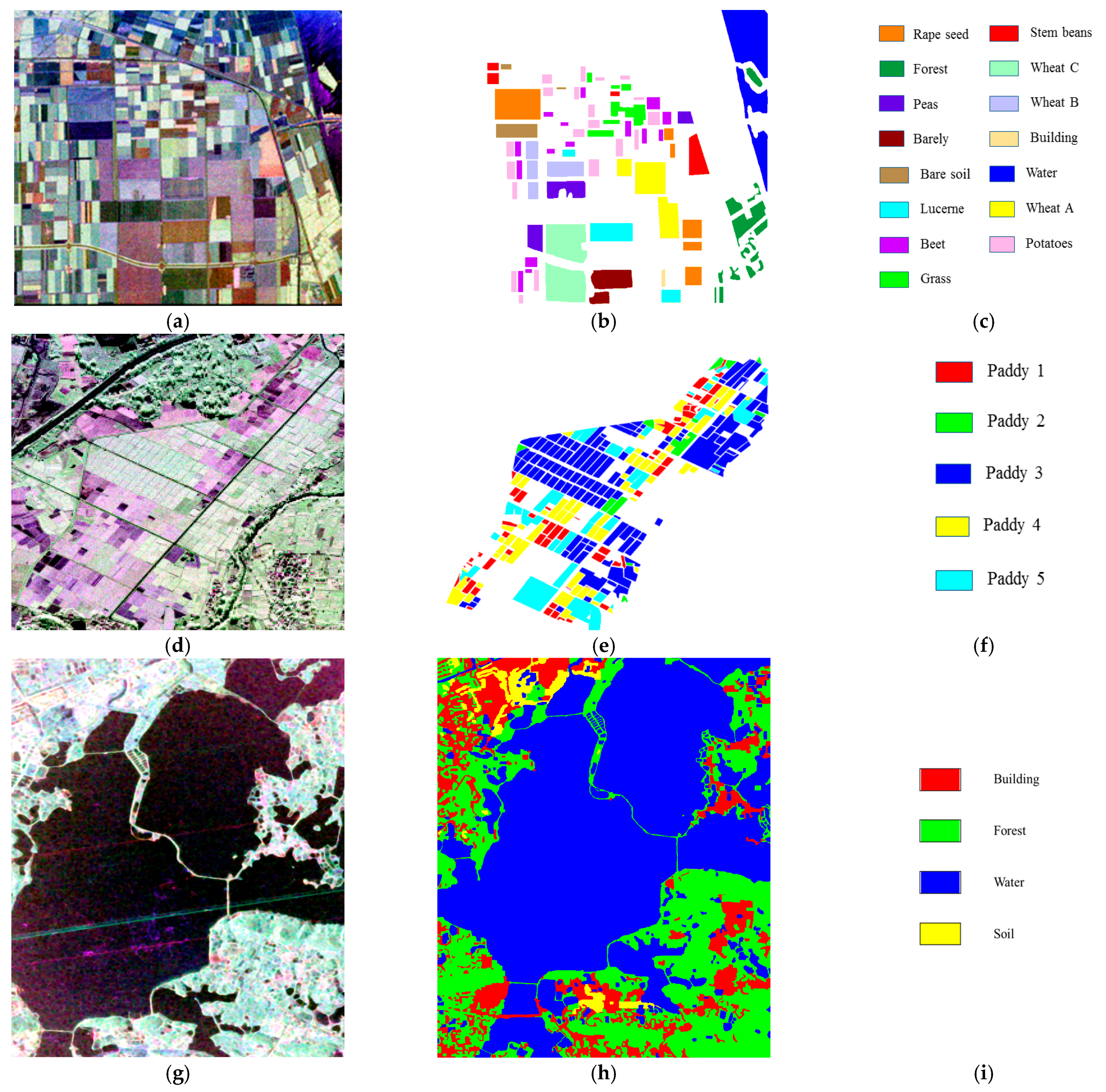
As shown in Figure 3a, PolSAR imagery is usually affected by speckle noise, which leads to the AIRSAR imagery to still have finely divided spots despite the speckle filtering in Figure 3b. For this reason, the GSRM algorithm is used to segment original AIRSAR image. To avoid the phenomenon of over-segmentation or under-segmentation, the segmentation parameters are set during the GSRM segmentation in this paper and we found the segmentation parameters which the scale parameter Q is 32 and the gradient threshold Δ is 0.5 can better retain details and preserve the shape of small land parcels than other scale parameters or gradient thresholds by visual assessment. The number of regions is 2235 and average number of pixels per region is 343, where the red line is the boundary of homogeneous area in Figure 3c. The result shows that GSRM segmentation can better suppress the influence of speckle noise than traditional filtering methods.
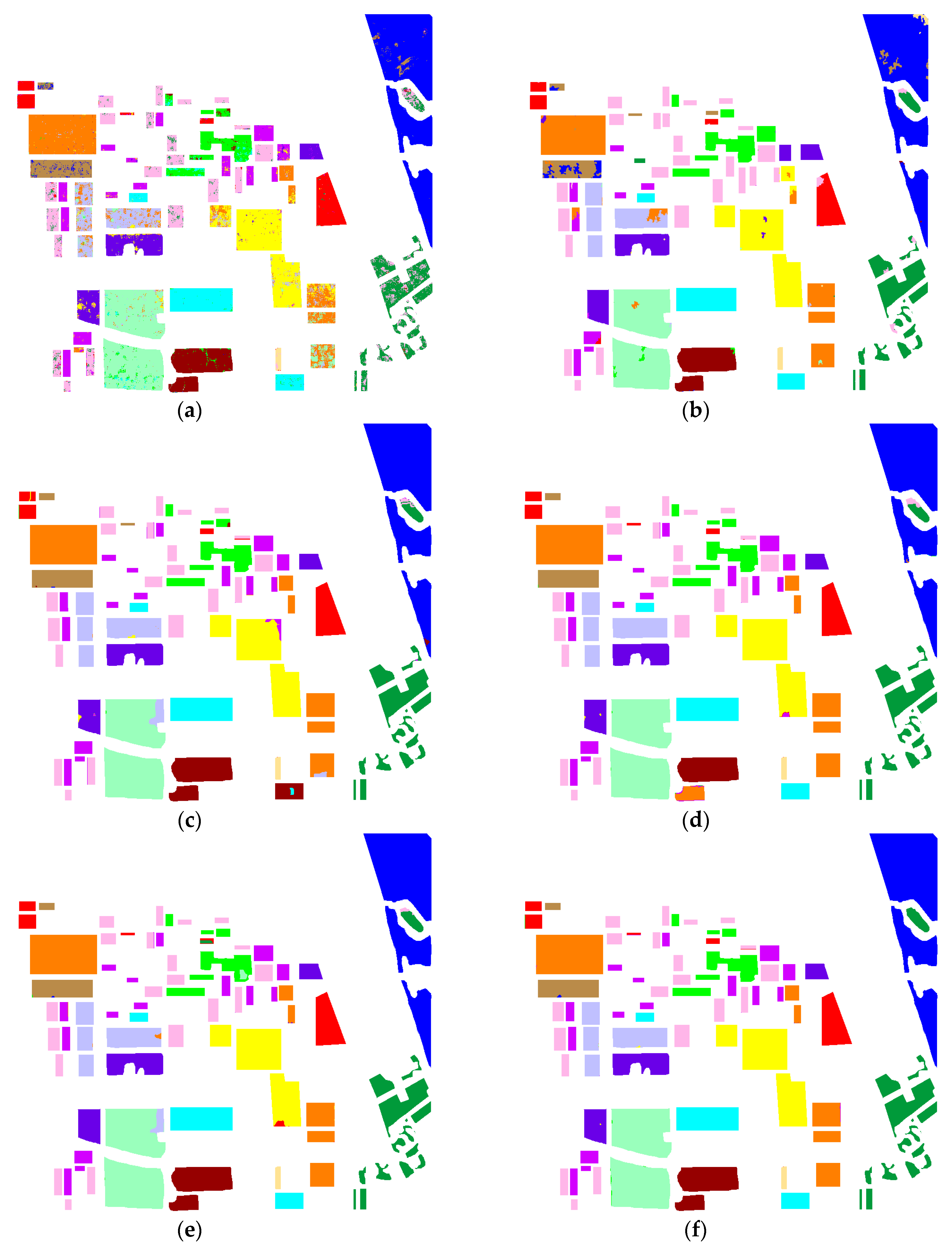
We designed several contrasting experiments to evaluate the effectiveness of the proposed method: Four different sample selection strategies (RS, MI, BT, and MBT) were considered first. In detail, we first randomly selected five training samples per class as the initial training set, which was done spatially by randomly selecting the segmented objects within a class and that all polarimetric parameters were considered in this step; in the second step, five samples per class were selected using the four different sample selection strategies (RS, MI, BT, and MBT) at each iteration, with the stopping criterion of the iteration set to 10 times; and the RF classifier was finally applied to identify the different types of land cover in the AIRSAR imagery. In addition, two other contrasting experiments were designed: (1) a pixel-based classification method using MBT strategies and RF classifier (named MBT_pixel); and (2) an object-based classification combined with MBT strategies and RF classifier, but it only uses the full T3 matrix (named MBT_T3). Figure 4 shows the classification results obtained with the AIRSAR imagery when 55 samples in each category are picked using the different strategies. It is noted that the training samples are used to train model of classification and test samples are used to evaluate the performance of the classification, so training samples used for classification accuracy assessment are independent of those used for algorithms training in this paper.
Table 2 lists the classification accuracies of each category, OA and Kappa of the classification results obtained for the AIRSAR imagery with the different strategies when 55 samples in each category are picked, which can be used to quantitatively compare the classification performances of different strategies.
As Figure 4 and Table 2 show, the object-based supervised classification methods can suppress the influence of speckle noise (MBT_pixel, OA 90.14% and Kappa 0.8915) and obtain pleasing classification performances when compared with the pixel-based supervised classification method. However, the performance with the RS strategy (OA 98.16% and Kappa 0.9798) is the worst among the different sample selection strategies when 55 samples in each category are picked, because the RS strategy randomly selects the training samples from the ground-truth maps, and the strategy does not consider the information contained in the training samples. The performances with MI (OA 98.62% and Kappa 0.9848) and BT (OA 99.24% and Kappa 0.9916) are better than the performance with RS strategy, as these methods adequately consider the information contained in the training samples. The MI strategy focuses on the most complicated area and the strategy of the BT algorithm focuses on the boundary area between the two most probable classes. As a result, these two methods are both prone to confusion and are less accurate than the MBT strategy (OA 99.74% and Kappa 0.9971) when the scenario is complicated. At the same time, the proposed method can fully use the polarimetric information and it can improve the performance when compared with the MBT_T3 (OA 94.42% and Kappa 0.9338) method.
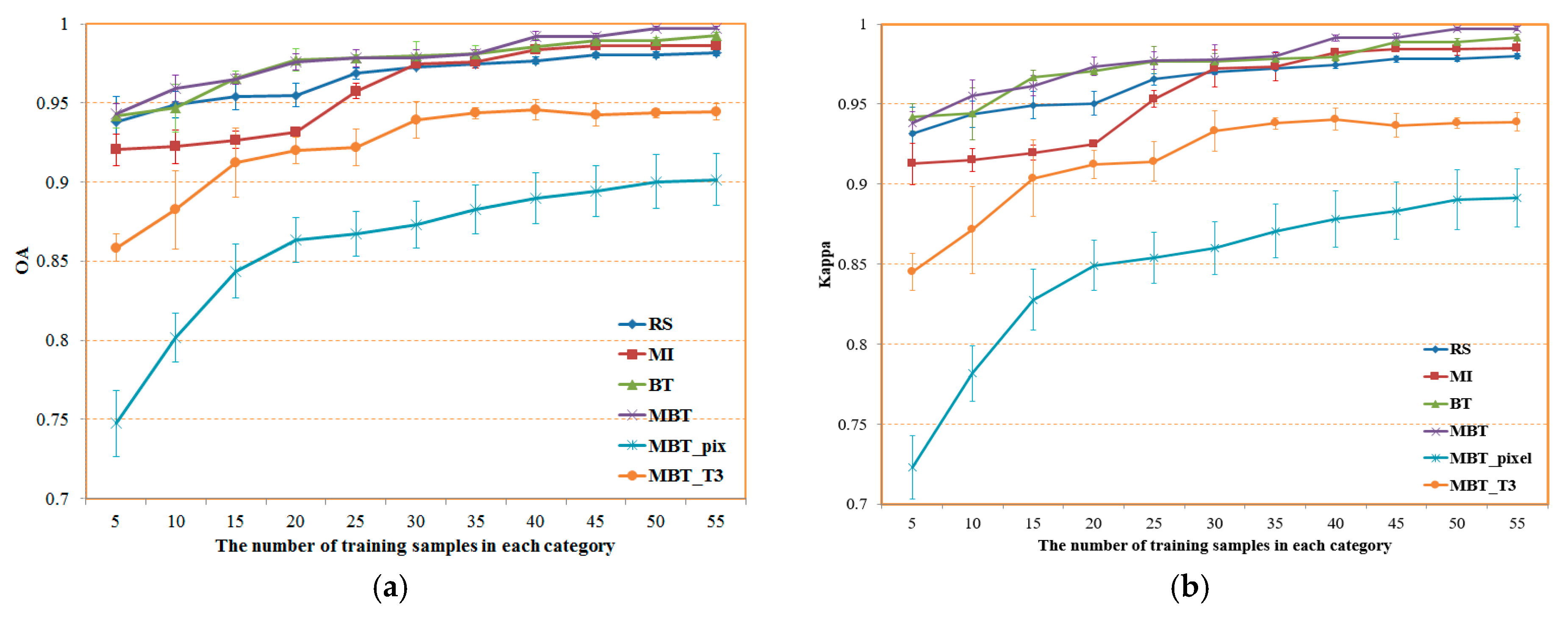
Figure 5 shows the classification accuracies with different numbers of training samples from the different strategies. The horizontal axis represents the number of training samples and the vertical axis represents the OA or Kappa. It can be seen that the classification performances become stable when the samples in each category are more than 50, and the performance of the MBT strategy is the best among the different strategies of sample selection when the samples in each category are more than 35.
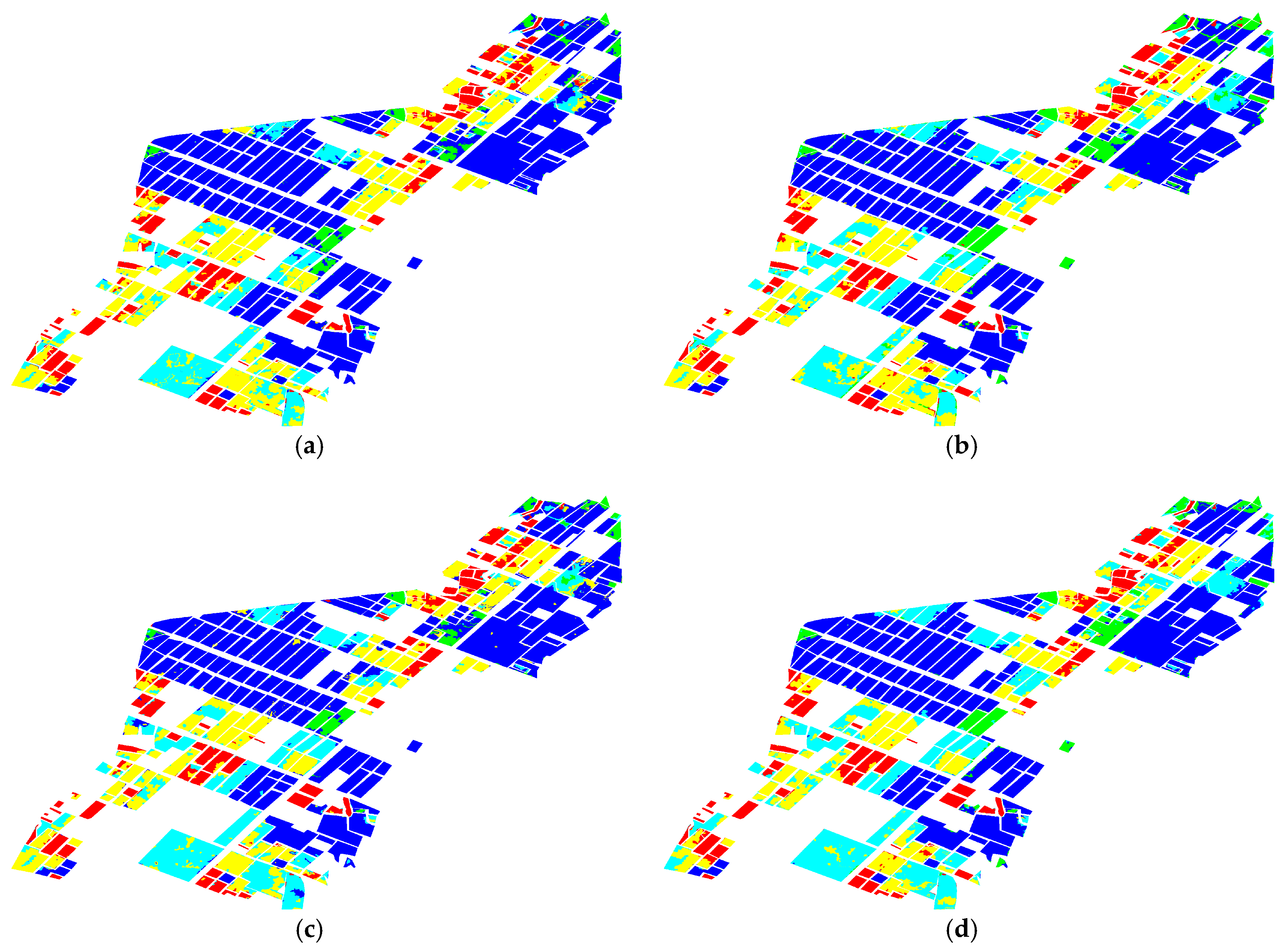
To quantitatively compare the classification results obtained by different classification algorithms, four different classification algorithms were considered: (1) k-nearest neighbor (KNN) classifier; (2) Wishart classifier; (3) LOR-LBP classifier; and (4) RF classifier. The four different classifiers are common classification algorithms of machine learning, which have been widely applied for the classification of PolSAR images. The KNN classifier is one of the most common classification algorithms in the remote sensing field [34]. The Wishart classifier is an important classifier based on the Wishart probability density function of PolSAR imagery [1]. The LOR-LBP classifier is a classifier based on Logistic regression via the loopy belief propagation (LBP) algorithm [13]. The RF classifier is an algorithm used to integrate multiple decision trees by the idea of ensemble learning [4].
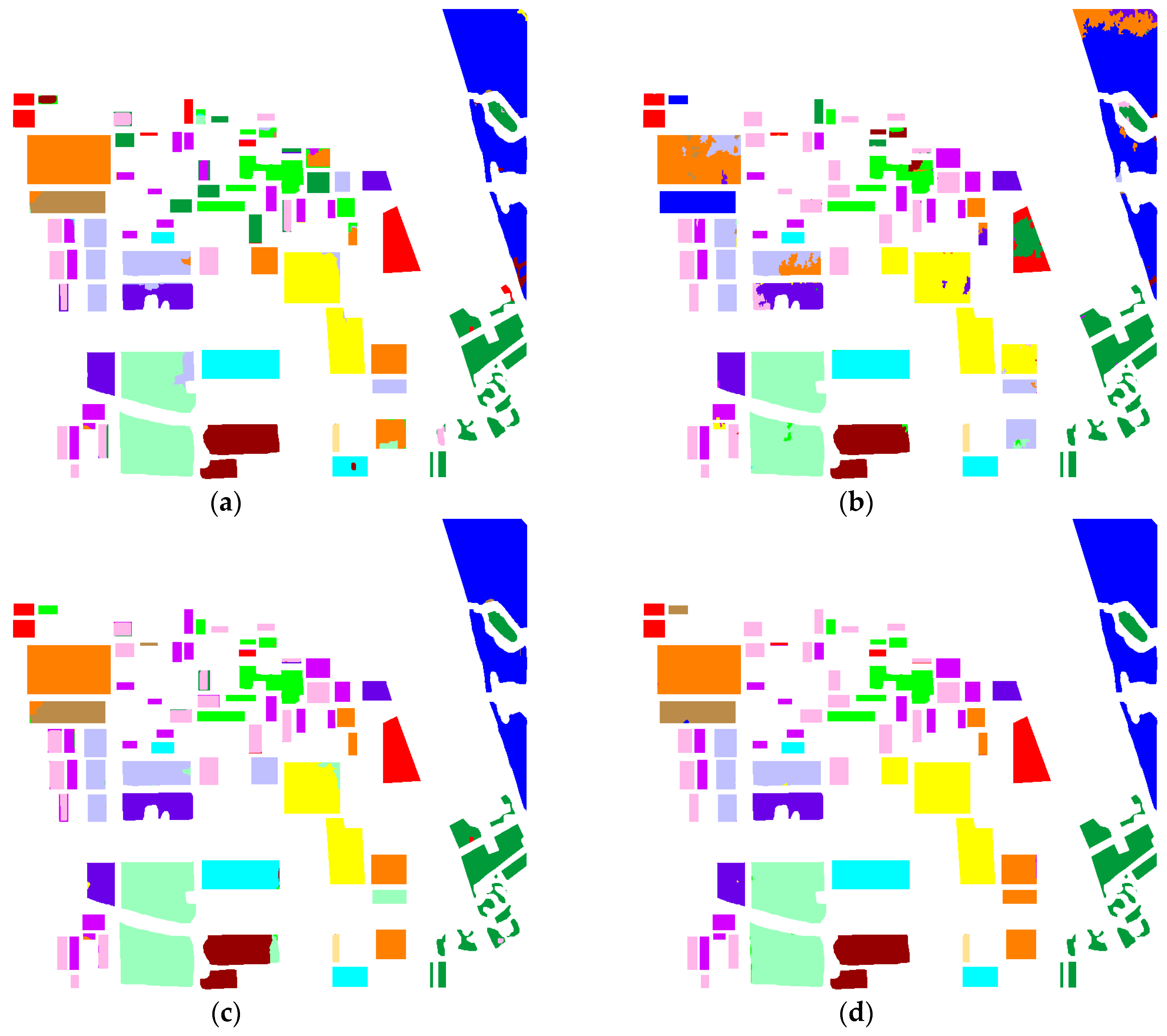
In detail, we first randomly selected five training samples per class as the initial training set, which was done spatially by randomly selecting the segmented objects within a class and that all the polarimetric parameters were considered in this step; in the second step, five samples per class were selected using the MBT strategy of sample selection at each iteration, with the stopping criterion of the iteration set to 10 times; and the four different classification algorithms were finally applied to identify the different types of land cover in the AIRSAR imagery. Figure 6 shows the classification results obtained with the AIRSAR imagery when 55 samples in each category are picked using the different classification algorithms.
Table 3 lists the classification performances (OA and Kappa) obtained for the AIRSAR imagery with the different classification algorithms when 55 samples in each category are picked, which can be used to quantitatively compare the classification results of different classification algorithms. The performance with the RF classifier (OA 99.74% and Kappa 0.9771) is the best among the different classification algorithms, which is because the RF classifier has strong generalization ability and also carries out the selection of implied features in the process of classification.
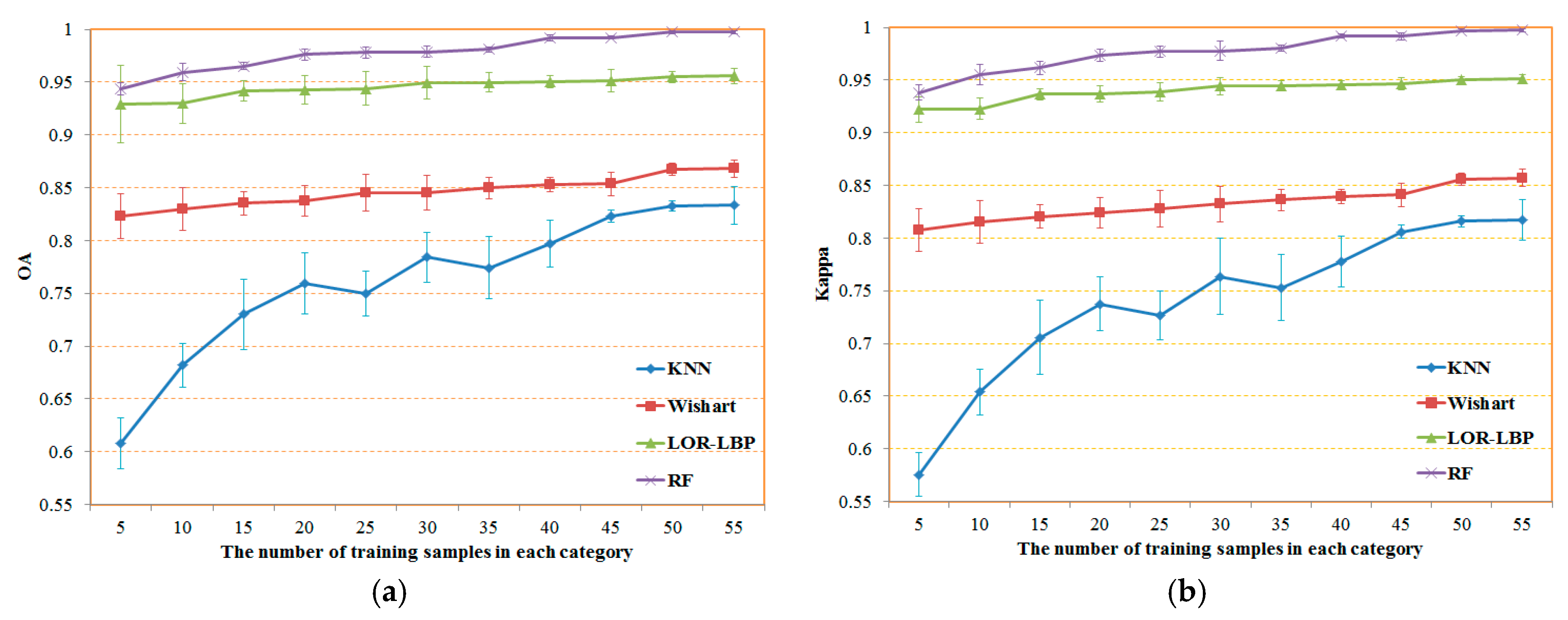
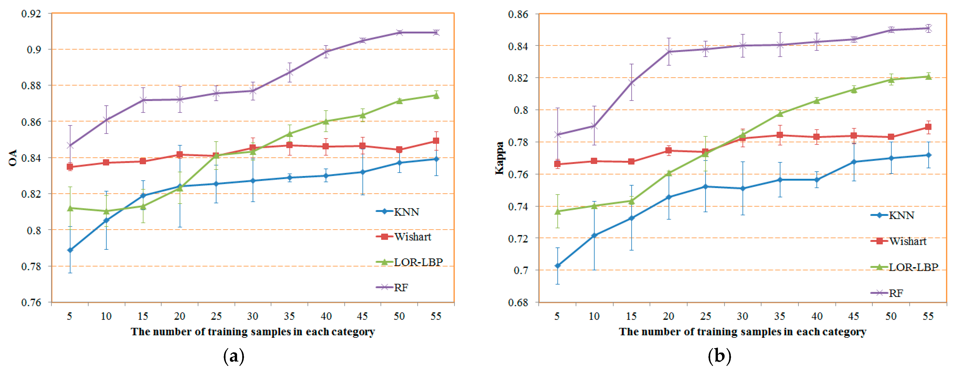
Figure 7 plots the classification accuracies of the different classification algorithms with different numbers of training samples. The horizontal axis represents the number of training samples, and the vertical axis represents the OA or Kappa of the different classification algorithms. Analogously, the classification performances become stable when the samples in each category are more than 40, and the performance with the RF classifier is the best among the different classification algorithms.
Several conclusions can be made from the results in Figure 4 and Figure 6. On the one hand, the proposed method (GSRM_MBT_RF) obtains the best performance (OA 99.74% and Kappa 0.9971) in all experiments, i.e., it can better suppress the speckle noise and obtain a higher OA and Kappa by taking full advantage of the polarimetric and spatial information. On the other hand, the performance using the MBT strategy is better than the other sample selection strategies, because the MBT strategy can more effectively select the labeled samples.
3.2.2. Experiments with UAVSAR Image
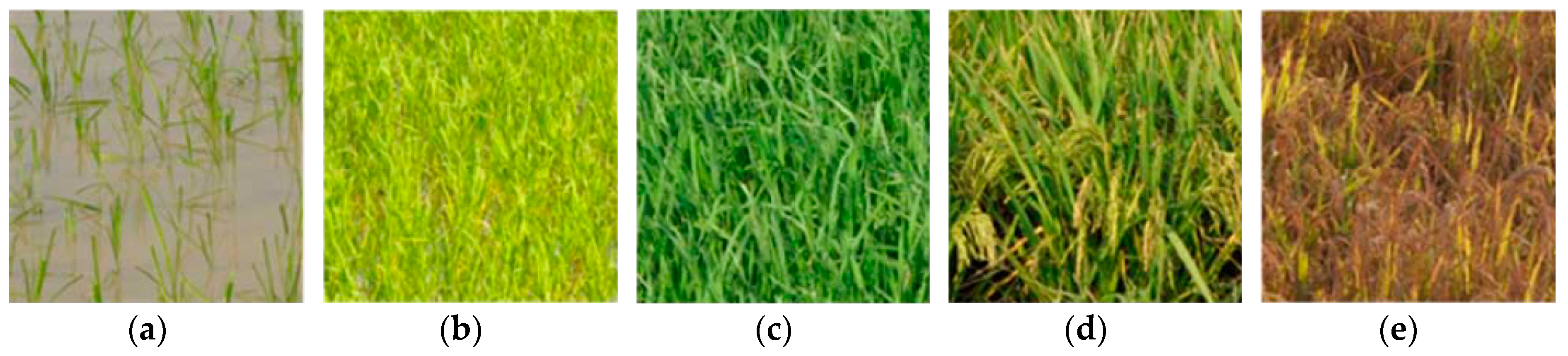
To further assess the effectiveness and feasibility of the proposed approach, a relatively complex situation (Paddy land from the city of Lingshui) was used to test the proposed approach. Five different growth stages of paddy (as shown in Figure 8) are researched in this situation, including stage of tillering, stem-elongation, panicle-exsertion, flowering and ripening. There are different heights and densities of paddies, so the performance of Radar cross-section (RCS) in UAVSAR imagery is different and it also leads to different polarimetric responses.
As shown in Figure 9a, UAVSAR imagery is more affected by speckle noise due to its high-resolution and leads to fewer scattering elements in the resolution unit of UAVSAR imagery. Therefore, the AIRSAR imagery still has finely divided spots despite the speckle filtering in Figure 9b. To suppress the influence of speckle noise, the GSRM algorithm is used to segment original UAVSAR imagery. The performance of segmentation is better when the scale parameter Q is 8 and the gradient threshold Δ is 4, by visual assessment. The number of regions is 11,836 and average number of pixels per region is 437. The result after GSRM segmentation is shown in Figure 9c and it shows that GSRM can better suppress the influence of speckle noise than traditional filtering method.
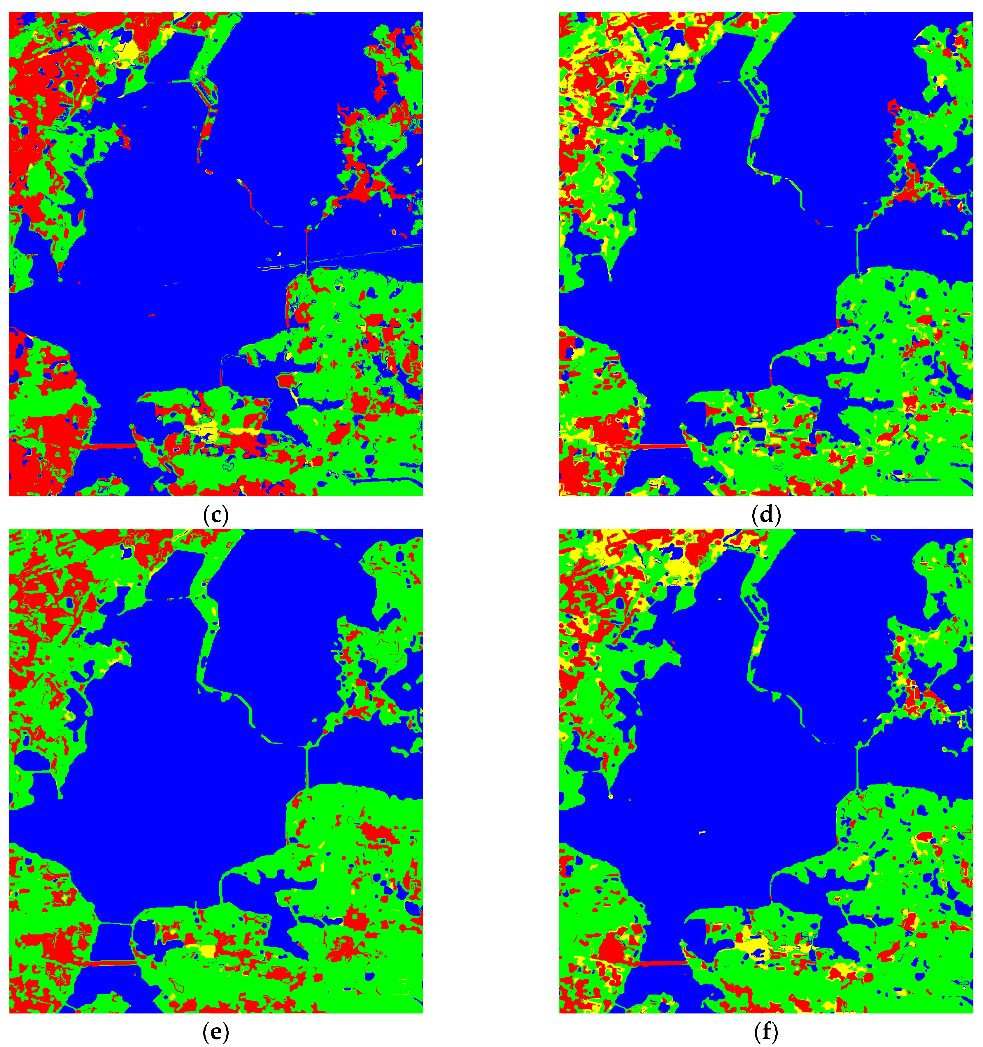
Similarly, four different sample selection strategies (RS, MI, BT, and MBT) were considered first. In detail, we first randomly selected five training samples in each category as the initial training set in these experiments, which was done spatially by randomly selecting the segmented objects within a class and that all the polarimetric parameters were considered in this step; in the second step, five samples in each category were selected using the four different sample selection strategies at each iteration, where the stopping criterion of the iteration was set to 10 times; and, finally, the RF classifier was applied to identify the different types of land cover in the PolSAR imagery. In addition, two other contrasting experiments were designed: (1) a pixel-based classification method using MBT strategies and RF classifier (named MBT_pixel); and (2) an object-based classification combined with MBT strategies and RF classifier, but it only uses the full T3 matrix (named MBT_T3). Figure 10 shows the classification results for the UAVSAR imagery when 55 samples in each category are picked from the different strategies.
Table 4 lists classification accuracies of each category and the classification results (OA and Kappa) for the UAVSAR imagery with the different strategies when 55 samples in each category are picked, which can be used to quantitatively compare the classification performances of different strategies.
Again, the experimental results demonstrate that the object-based supervised classification methods can suppress the influence of speckle noise (MBT_pixel, OA 77.04% and Kappa 0.7516) and obtain pleasing classification performances, as shown in Figure 10 and Table 4. Meanwhile, the performance with the RS strategy (OA 87.94% and Kappa 0.8207) is the worst among the different strategies. This is because the RS strategy randomly selects the training samples from the ground-truth maps, and the RS strategy does not consider the information contained in the training samples. The performances with MI (OA 88.56% and Kappa 0.8349) and BT (OA 88.73% and Kappa 0.8372) are better than the performance with RS, which is because the former strategies adequately consider the information contained in the training samples. However, the MI strategy focuses on the most complicated area, and the BT algorithm strategy focuses on the boundary area between the two most probable classes, so these methods are prone to confusion and are less accurate than the MBT strategy (OA 90.93% and Kappa 0.8509). At the same time, the proposed method can fully use the polarimetric information and it can improve the performance when compared with the MBT_T3 method (OA 87.25% and Kappa 0.8317).
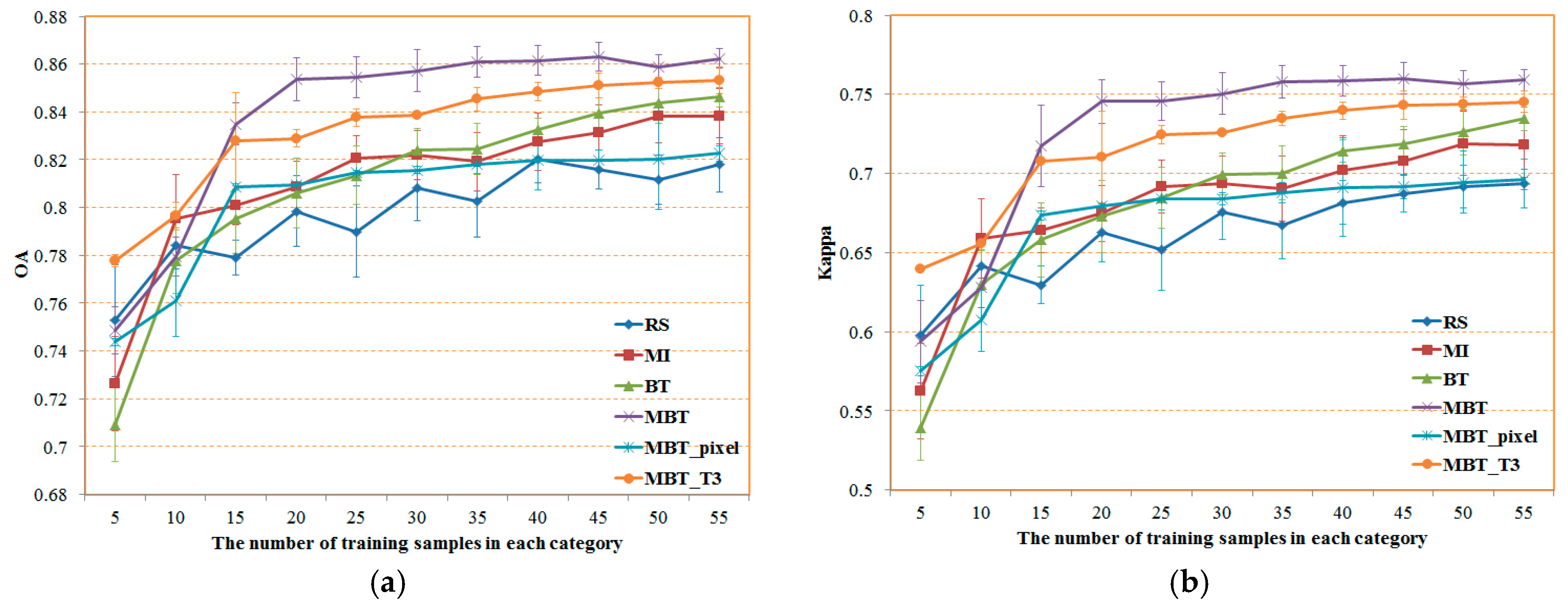
Figure 11 shows the classification accuracy with different numbers of training samples from the different strategies. The horizontal axis represents the number of training samples, and the vertical axis represents the OA or Kappa of the different sample selection strategies. The classification performances become stable when the samples in each category are more than 50, and the performance of the proposed method is the best among the different strategies.
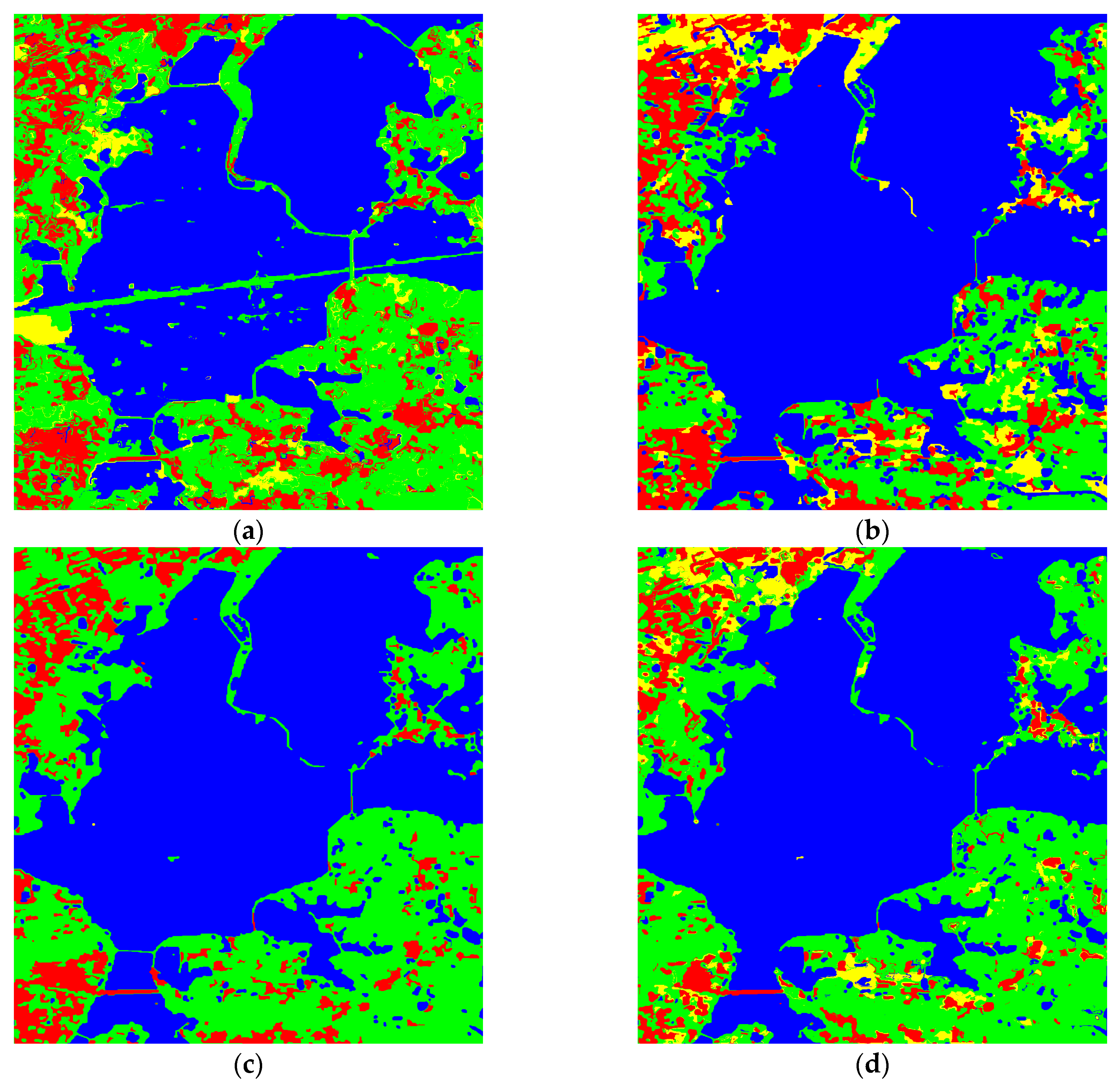
To quantitatively compare the classification results with different classification algorithms, four different classification algorithms were also considered. In detail, we first randomly selected five training samples per class as the initial training set, which was done spatially by randomly selecting the segmented objects within a class and that all the polarimetric parameters were considered in this step; in the second step, five samples per class were selected using the MBT strategy of sample selection at each iteration, with the stopping criterion of the iteration set to 10 times; and the four different classification algorithms were finally applied to identify the different types of land cover in the UAVSAR imagery. Figure 12 shows the classification results obtained with the UAVSAR imagery when 55 samples in each category are picked using the different classification algorithms.
Table 5 lists the classification results (OA and Kappa) for the UAVSAR imagery with the different classification algorithms when 55 samples in each category are picked, which can be used to quantitatively compare the classification results of different classification algorithms. The performance with RF (OA 90.93% and Kappa 0.8509) is the best among the different classification algorithms, which is because the RF classifier has strong generalization ability and also carries out the selection of implied features in the process of classification.
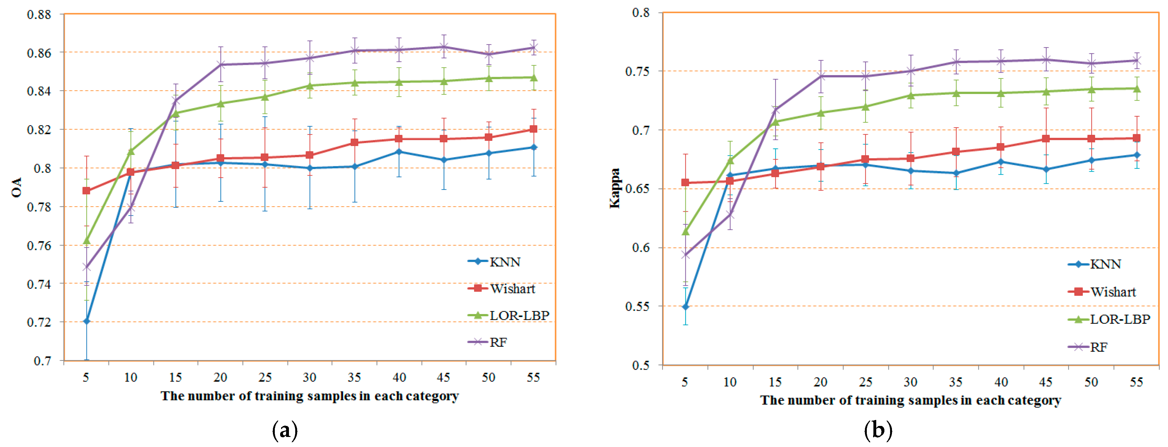
Figure 13 shows the classification accuracies with different numbers of training samples from the different classification algorithms. The horizontal axis represents the number of training samples, and the vertical axis represents the OA or Kappa of the different classification algorithms. Analogously, the performance with the RF classifier remains the best among the different classification algorithms.
Analogously, several conclusions can be made from the results in Figure 10 and Figure 12. On the one hand, the proposed method obtains the best performance (OA 90.93% and Kappa 0.8509) in all the experiments, i.e., it can better suppress the speckle noise and obtain a higher OA and Kappa by taking full advantage of the polarimetric and spatial information. On the other hand, the performance with the MBT strategy is better than the other sample selection strategies, because the MBT strategy can more effectively select the labeled samples.
3.2.3. Experiments with RadarSat-2 Image
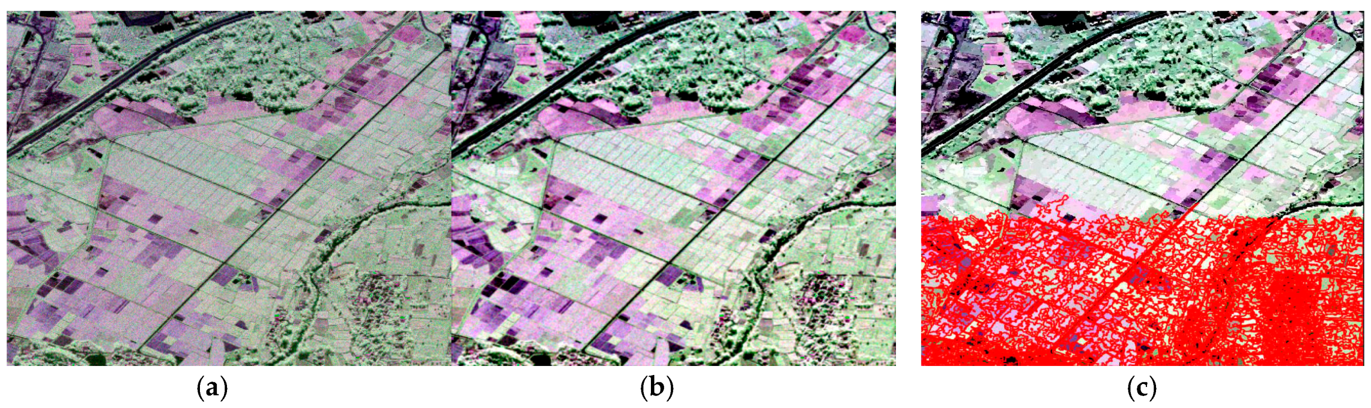
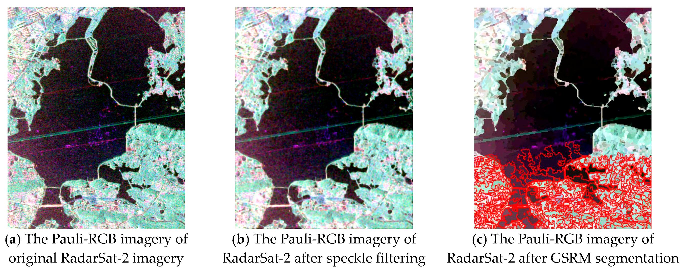
To further assess the effectiveness and feasibility of the proposed approach, an actual urban scene (the city of Wuhan, China) was used to test the proposed approach. To avoid the influence of speckle noise, filtering method and GSRM algorithm were applied to original RadarSat-2 image. The segmentation parameters were set during the GSRM segmentation and we found the segmentation parameters when the scale parameter Q is 16 and the gradient threshold Δ is 0.5 can better retain details and preserve the shape of small land parcels than other scale parameters or gradient thresholds by visual assessment. The number of regions is 4135 and average number of pixels per region is 283. The result after GSRM segmentation (Figure 14c) shows that GSRM segmentation can better suppress the influence of speckle noise than traditional filtering methods.
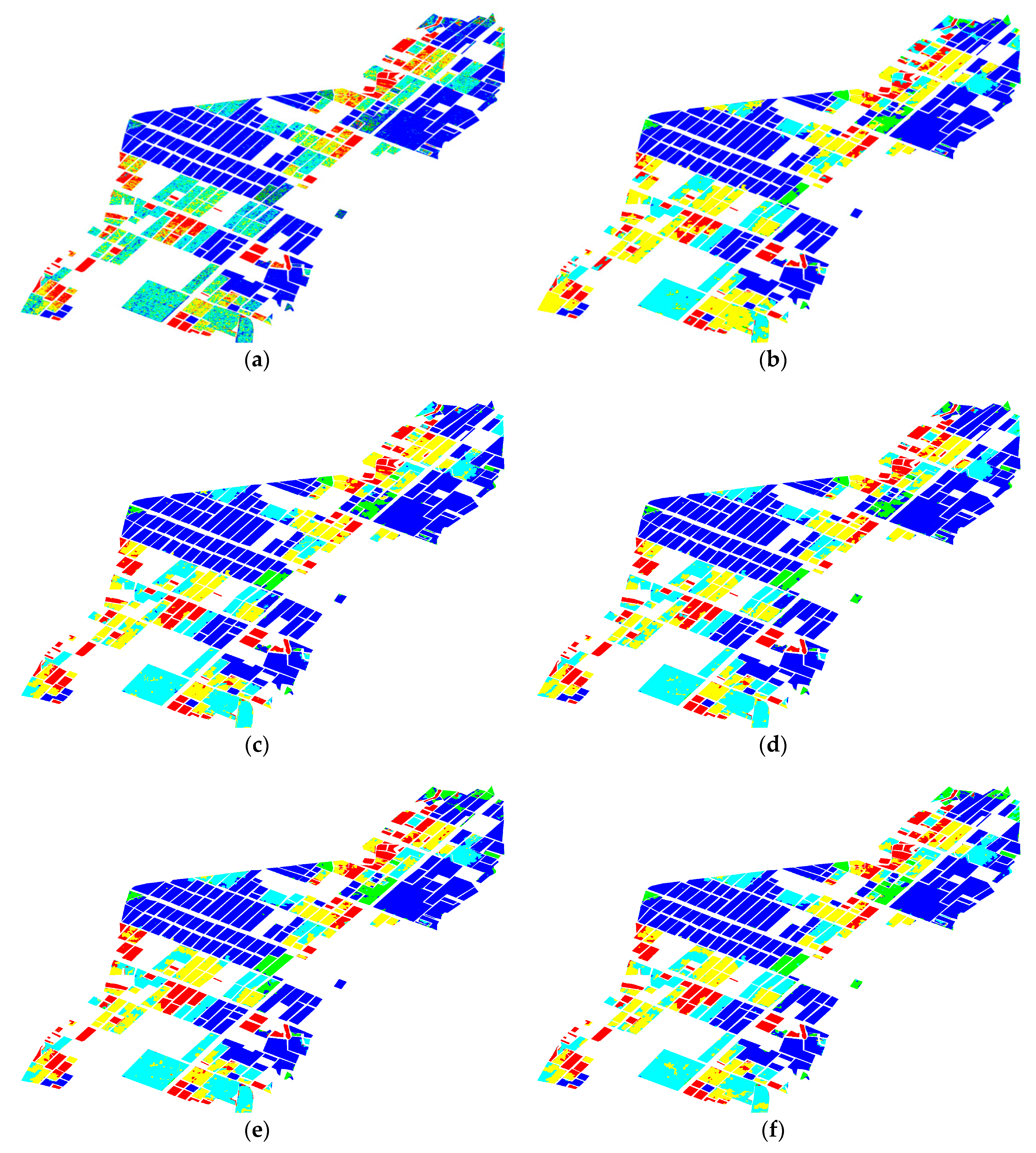
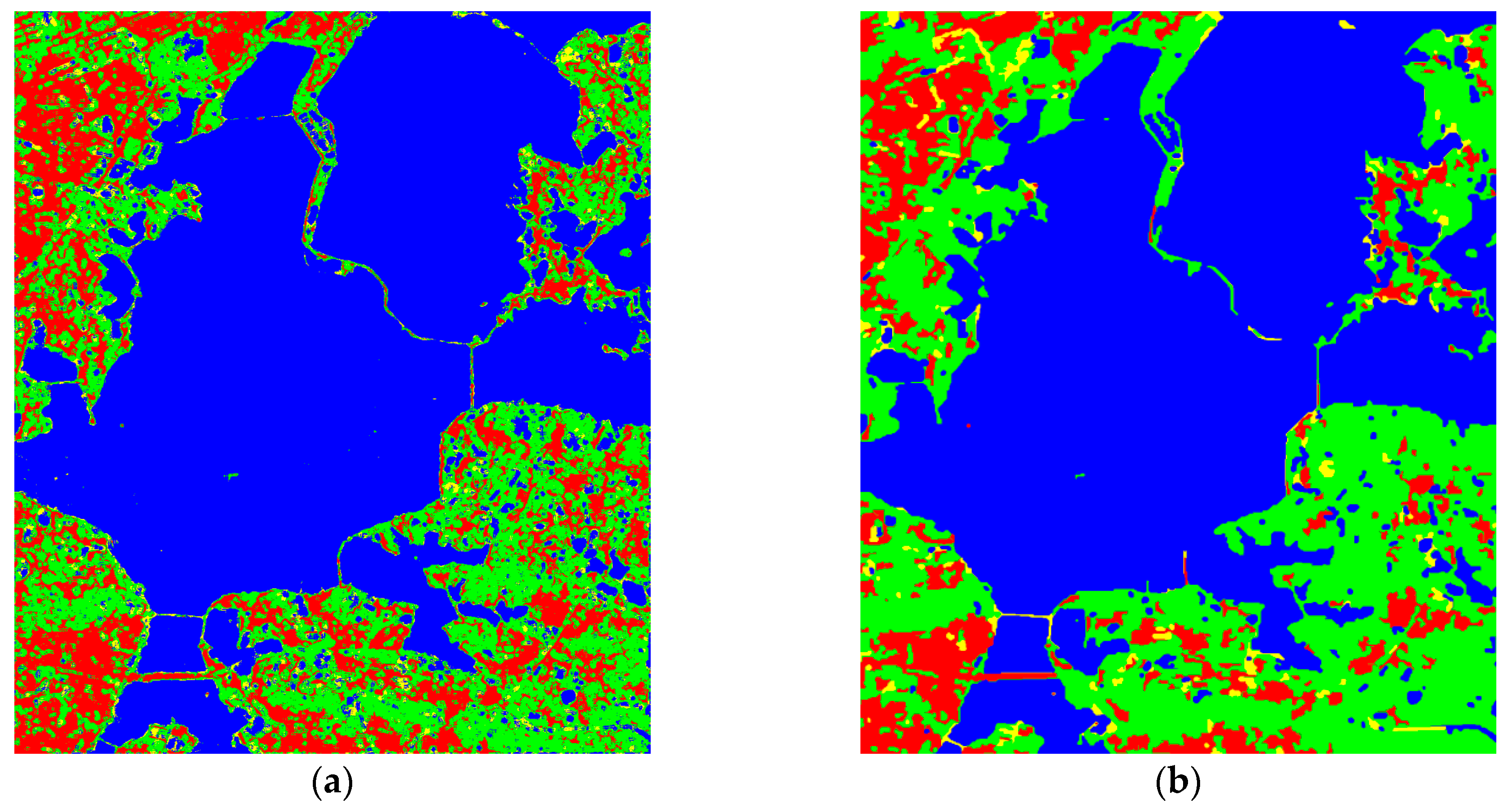
Similarly, four different sample selection strategies were considered first. In detail, we still first randomly selected five training samples in each category as the initial training set in these experiments, which was done spatially by randomly selecting the segmented objects within a class and that all the polarimetric parameters were considered in this step; in the second step, five samples in each category were selected using the four different sample selection strategies at each iteration, where the stopping criterion of the iteration was set to 10 times; and, finally, the RF classifier was applied to identify the different types of land cover in the PolSAR imagery. In addition, two other contrasting experiments were designed: (1) a pixel-based classification method using MBT strategies and RF classifier (named MBT_pixel); and (2) an object-based classification combined with MBT strategies and RF classifier, but it only uses the full T3 matrix (named MBT_T3). Figure 15 shows the classification results for the RadarSat-2 imagery when 55 samples in each category are picked from the different strategies.
Table 6 lists classification accuracies of each category and the classification results (OA and Kappa) for the RadarSat-2 imagery with the different strategies when 55 samples in each category are picked, which can be used to quantitatively compare the classification performances of different strategies.
Again, the experimental results demonstrate that the object-based supervised classification methods can suppress the influence of speckle noise (MBT_pixel, OA 82.26% and Kappa 0.6959) and obtain pleasing classification performances, as shown in Figure 15 and Table 6. Meanwhile, the performance with the RS strategy (OA 81.79% and Kappa 0.6936) is the worst among the different sample selection strategies. This is because the RS strategy randomly selects the training samples from the ground-truth maps, and the RS strategy does not consider the information contained in the training samples. The performances with MI (OA 83.82% and Kappa 0.7180) and BT (OA 84.64% and Kappa 0.7345) are better than the performance with RS, which is because the former strategies adequately consider the information contained in the training samples. However, the MI strategy focuses on the most complicated area, and the BT algorithm strategy focuses on the boundary area between the two most probable classes, so these methods are prone to confusion and are less accurate than the MBT strategy (OA 86.23% and Kappa 0.7590). The proposed method fully use the polarimetric information and it can improve the performance when compared with the MBT_T3 method (OA 84.86% and Kappa 0.7398).
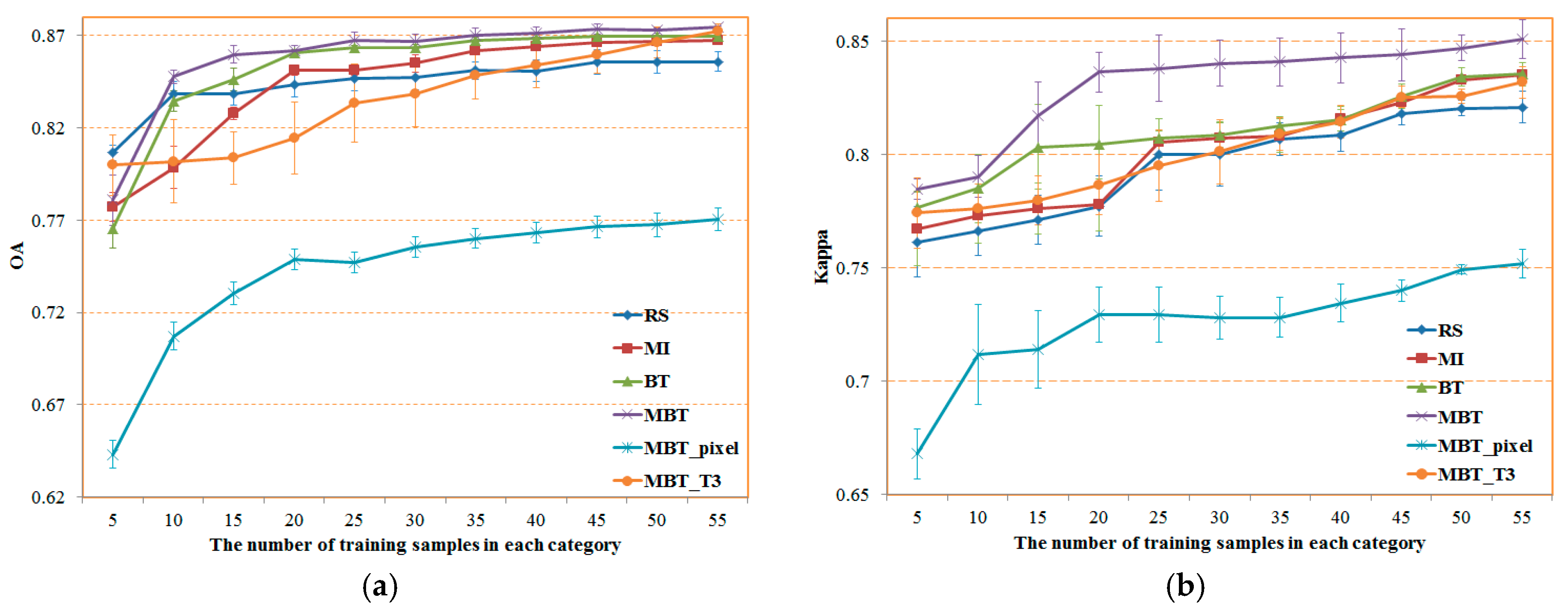
Figure 16 shows the classification accuracy with different numbers of training samples from the different strategies. The horizontal axis represents the number of training samples, and the vertical axis represents the OA or Kappa of the different sample selection strategies. The classification performances become stable when the samples in each category are more than 50, and the performance with the proposed method is the best among the different strategies.
To quantitatively compare the classification results with different classification algorithms, four different classification algorithms were also considered. In detail, we first randomly selected five training samples per class as the initial training set in these experiments, which was done spatially by randomly selecting the segmented objects within a class and that all the polarimetric parameters were considered in this step; in the second step, five samples per class were selected using the MBT strategy of sample selection at each iteration, with the stopping criterion of the iteration set to 10 times; and the four different classification algorithms were finally applied to identify the different types of land cover in the RadarSat-2 imagery. Figure 17 shows the classification results obtained with the RadarSat-2 imagery when 55 samples in each category are picked using the different classification algorithms.
Table 7 lists the classification results (OA and Kappa) for the RadarSat-2 imagery with the different classification algorithms when 55 samples in each category are picked, which can be used to quantitatively compare the classification results of different classification algorithms. The performance with RF (OA 86.23% and Kappa 0.7590) is the best among the different classification algorithms, which is because the RF classifier has strong generalization ability and also carries out the selection of implied features in the process of classification.
Figure 18 shows the classification accuracies with different numbers of training samples from the different classification algorithms. The horizontal axis represents the number of training samples, and the vertical axis represents the OA or Kappa of the different classification algorithms. Analogously, the performance with the RF classifier remains the best among the different classification algorithms.
Analogously, several conclusions can be made from the results in Figure 16 and Figure 18. On the one hand, the proposed method obtains the best performance (OA 86.23% and Kappa 0.7590) in all the experiments, i.e., it can better suppress the speckle noise and obtain a higher OA and Kappa by taking full advantage of the polarimetric and spatial information. On the other hand, the performance with the MBT strategy is better than the other sample selection strategies, because the MBT strategy can more effectively select the labeled samples.
4. Discussion
Most state-of-the-art supervised classification methods using PolSAR imagery are limited by the availability of effective training samples, and the results of the traditional pixel-based supervised classification methods are subject to the influence of speckle noise. In this paper, to solve the problems of existing supervised classification methods when using PolSAR data, we have proposed an object-based supervised classification method (GSRM_MBT_RF), which combines the advantages of the GSRM algorithm, the AL method, and the RF classifier. The experimental results indicated that the proposed approach achieves the best performances with regard to OA and Kappa. Moreover, the proposed method can not only better suppress the speckle noise, but can also perform well when the training samples are limited.
The accuracies of experiments from different sensors are different by proposed method and the sources of the results mainly include that: (1) The resolution of PolSAR imagery is different. The UAVSAR is high-resolution and it leads to the fewer scattering elements in the resolution unit of UAVSAR imagery. Nevertheless, the AIRSAR imagery and RadarSat-2 imagery are medium resolution and they are relatively simple. (2) The categories of PolSAR imagery are different. The AIRSAR imagery and UAVSAR imagery mainly focus on agricultural field. The categories of AIRSAR imagery are entirely different and it leads to different polarization responses. However, the categories of UAVSAR imagery are five different growth stages of paddy and it might bring about the confusion in classification procedures. The RadarSat-2 imagery is urban scene and the situation is relatively complex. (3) The influence of topography is different. The city of Wuhan has an undulating relief and it is prone to misclassification.
The proposed method has several advantages when compared with the traditional supervised classification methods for PolSAR data: (1) The proposed method can obtain obviously higher classification accuracy when compared with pixel-based supervised classification methods, due to using the GSRM algorithm to better suppress the influence of speckle noise. (2) The proposed method considers the maximum information of the training samples and more effectively selects the labeled samples by the AL method. This allows the proposed method to perform well, even when the training samples are limited. (3) The RF classifier integrates a feature evaluation technique, so that it is not necessary to carry out feature selection. (4) The proposed approach takes full advantage of the polarimetric information and spatial information of PolSAR imagery. As a result, it can obtain a better OA and Kappa when compared with the traditional supervised classification methods.
However, the proposed method still has some disadvantages: (1) the redundancy of polarimetric features might pollute the classifier and it is necessary to analyze and select the most relevant features before implementation of proposed method; and (2) the algorithm structure is relatively complex and time-consuming when compared with the state-of-the-art supervised classification methods.
5. Conclusions
A novel object-based supervised classification method for PolSAR imagery is proposed in this paper. The first step of the proposed method is aimed at reducing the speckle noise through the GSRM algorithm. A reliable training set is then selected from the different polarimetric features of the PolSAR imagery by the AL method. Finally, the RF classifier is applied to identify the different types of land cover. To validate the performance of the proposed method, three PolSAR datasets acquired by different sensors were considered, and the experimental results showed that the proposed method significantly improves the classification accuracy for PolSAR images. Meanwhile, four different sample selection strategies and four different classification algorithms were applied to assess the effectiveness and feasibility of the proposed method. The analysis showed that the proposed method can not only better suppress the speckle noise, but can also significantly improve the OA and Kappa, even when the training samples are limited. Nevertheless, further investigation is still necessary. For example, in our future work, it is necessary to suppress the effect of terrain for classification using relevant DEM data, and the proposed method should be optimized by considering feature optimization.
Author Contributions
W.L. defined the research problem, proposed the methods, undertook most of the programming, and wrote the paper. J.Y. gave some key advice. P.L. gave useful advice and contributed to the paper writing. Y.H. contributed to the paper writing and provided the ground truth. J.Z. contributed to the paper writing. H.S. collected the data and processed the datasets.
Funding
This research was funded by the National Natural Science Foundation of China (No. 91438203, No. 61371199, No. 41501382, and No. 41601355), the Hubei Provincial Natural Science Foundation (No. 2015CFB328 and No. 2016CFB246), the National Basic Technology Program of Surveying and Mapping (No. 2016KJ0103), and the Technology of Target Recognition Based on GF-3 Program (No. 03-Y20A10-9001-15/16).
Conflicts of Interest
The authors declare no conflict of interest.
References
- Lee, J.S.; Grunes, M.R.; Kwok, R. Classification of multi-look polarimetric SAR imagery based on complex Wishart distribution. Int. J. Remote. Sens. 1994, 15, 2299–2311. [Google Scholar] [CrossRef]
- Martinuzzi, S.; Gould, W.A.; González, O.M.R. Land development, land use, and urban sprawl in Puerto Rico integrating remote sensing and population census data. Landsc. Urban Plan. 2007, 79, 288–297. [Google Scholar] [CrossRef]
- Zhao, L.; Yang, J.; Li, P. Damage assessment in urban areas using post-earthquake airborne PolSAR imagery. Int. J. Remote. Sens. 2013, 34, 8952–8966. [Google Scholar] [CrossRef]
- Sun, W.; Li, P.; Yang, J. Polarimetric SAR image classification using a wishart test statistic and a wishart dissimilarity measure. IEEE Geosci. Remote Sens. Lett. 2017, 14, 1–5. [Google Scholar] [CrossRef]
- Zhao, L.; Yang, J.; Li, P. Seasonal inundation monitoring and vegetation pattern mapping of the Erguna floodplain by means of a RADARSAT-2 fully polarimetric time series. Remote Sens. Environ. 2014, 152, 426–440. [Google Scholar] [CrossRef]
- Shi, L.; Zhang, L.; Yang, J. Supervised graph embedding for polarimetric SAR image classification. IEEE Geosci. Remote Sens. Lett. 2013, 10, 216–220. [Google Scholar] [CrossRef]
- Qi, Z.; Yeh, A.G.-O.; Li, X. A novel algorithm for land use and land cover classification using RADARSAT-2 polarimetric SAR data. Remote Sens. Environ. 2012, 118, 21–39. [Google Scholar] [CrossRef]
- Maggiori, E.; Tarabalka, Y.; Charpiat, G.; Alliez, P. Convolutional neural networks for large-scale remote-sensing image classification. IEEE Trans. Geosci. Remote Sens. 2017, 55, 645–657. [Google Scholar] [CrossRef]
- Samat, A.; Gamba, P.; Du, P. Active extreme learning machines for quad-polarimetric SAR imagery classification. Int. J. Appl. Earth Obs. Geoinf. 2015, 35, 305–319. [Google Scholar] [CrossRef]
- Mahdianpari, M.; Salehi, B.; Mohammadimanesh, F. Random forest wetland classification using ALOS-2 L-band, RADARSAT-2 C-band, and TerraSAR-X imagery. ISPRS J. Photogramm. Remote Sens. 2017, 130, 13–31. [Google Scholar] [CrossRef]
- Li, J.; Bioucas-Dias, J.M.; Plaza, A. Hyperspectral image segmentation using a new bayesian approach with active learning. IEEE Trans. Geosci. Remote Sens. 2011, 49, 3947–3960. [Google Scholar] [CrossRef]
- Rajan, S.; Ghosh, J.; Crawford, M.M. An active learning approach to hyperspectral data classification. IEEE Trans. Geosci. Remote Sens. 2008, 46, 1231–1242. [Google Scholar] [CrossRef]
- Li, J.; Bioucas-Dias, J.M.; Plaza, A. Spectral–spatial classification of hyperspectral data using loopy belief propagation and active learning. IEEE Trans. Geosci. Remote Sens. 2013, 51, 844–856. [Google Scholar] [CrossRef]
- Lee, J.S.; Pottier, E. Polarimetric Radar Imaging From Basics to Applications; CRC Press: Boca Raton, FL, USA, 2017. [Google Scholar]
- Cloude, S.R.; Pottier, E. A review of target decomposition theorems in radar polarimetry. IEEE Trans. Geosci. Remote Sens. 1996, 34, 498–518. [Google Scholar] [CrossRef]
- Cloude, S.R. Target decomposition theorems in radar scattering. Electron. Lett. 1985, 21, 22–24. [Google Scholar] [CrossRef]
- Freeman, A.; Durden, S.L. A three-component scattering model for polarimetric SAR data. IEEE Trans. Geosci. Remote Sens. 1998, 36, 963–973. [Google Scholar] [CrossRef]
- Van Zyl, J.J. Application of Cloude’s target decomposition theorem to polarimetric imaging radar data. In Radar Polarimetry; Bellingham: Washington, DC, USA, 1993; Volume 1748, pp. 184–192. [Google Scholar]
- Park, S.-E.; Yamaguchi, Y.; Kim, D.-J. Polarimetric SAR remote sensing of the 2011 Tohoku earthquake using ALOS/PALSAR. Remote Sens. Environ. 2013, 132, 212–220. [Google Scholar] [CrossRef]
- Touzi, R. Target scattering decomposition in terms of roll-invariant target parameters. IEEE Trans. Geosci. Remote Sens. 2007, 45, 73–84. [Google Scholar] [CrossRef]
- Arii, M.; van Zyl, J.J.; Kim, Y. Adaptive model-based decomposition of polarimetric SAR covariance matrices. IEEE Trans. Geosci. Remote Sens. 2011, 49, 1104–1113. [Google Scholar] [CrossRef]
- Qin, F.; Guo, J.; Sun, W. Object-oriented ensemble classification for polarimetric SAR imagery using restricted Boltzmann machines. Remote Sens. Lett. 2016, 8, 204–213. [Google Scholar] [CrossRef]
- Ma, L.; Li, M.; Ma, X. A review of supervised object-based land-cover image classification. ISPRS J. Photogramm. Remote Sens. 2017, 130, 277–293. [Google Scholar] [CrossRef]
- Lang, F.; Yang, J.; Li, D.; Zhao, L.; Shi, L. Polarimetric SAR image segmentation using statistical region merging. IEEE Geosci. Remote Sens. Lett. 2014, 11, 509–513. [Google Scholar] [CrossRef]
- Comaniciu, D.; Meer, P. Mean shift: A robust approach toward feature space analysis. IEEE Trans Pattern Anal. Mach. Intell. 2002, 24, 603–619. [Google Scholar] [CrossRef]
- Qin, F.; Guo, J.; Lang, F. Superpixel segmentation for polarimetric SAR imagery using local iterative clustering. IEEE Geosci. Remote Sens. Lett. 2017, 12, 13–17. [Google Scholar]
- Xiang, D.; Ban, Y.; Wang, W. Adaptive superpixel generation for polarimetric SAR images with local iterative clustering and SIRV model. IEEE Trans. Geosci. Remote Sens. 2017, 55, 3115–3131. [Google Scholar] [CrossRef]
- Liu, W.; Yang, J.; Zhao, J. A novel method of unsupervised change detection using multi-temporal PolSAR images. Remote Sens. 2017, 9, 1135. [Google Scholar] [CrossRef]
- Zhang, L.; Li, A.; Li, X. Remote sensing image segmentation based on an improved 2-D gradient histogram and MMAD model. IEEE Geosci. Remote Sens. Lett. 2015, 12, 58–62. [Google Scholar] [CrossRef]
- Nock, R.; Nielsen, F. Statistical region merging. IEEE Trans. Pattern Anal. Mach. Intell. 2004, 26, 1452. [Google Scholar] [CrossRef] [PubMed]
- Luo, T.; Kramer, K.; Goldgof, D.B.; Hall, L.O.; Samson, S.; Remsen, A.; Hopkins, T. Active learning to recognize multiple types of plankton. J. Mach. Learn. Res. 2005, 6, 589–613. [Google Scholar]
- Tuia, D.; Ratle, F.; Pacifici, F. Active learning methods for remote sensing image classification. IEEE Trans. Geosci. Remote Sens. 2009, 47, 2218–2232. [Google Scholar] [CrossRef]
- Tuia, D.; Volpi, M.; Copa, L.; Kanevski, M.; Munoz-Mari, J. A survey of active learning algorithms for supervised remote sensing image classification. IEEE J. Sel. Top. Signal Process. 2011, 5, 606–617. [Google Scholar] [CrossRef]
- Hastie, T.; Tibshirani, R. Discriminant adaptive nearest neighbor classification and regression. IEEE Trans. Pattern Anal. Mach. Intell. 1996, 18, 409–415. [Google Scholar] [CrossRef]
Figure 1.
The process flow of the proposed method.

Figure 2.
Pauli-RGB images of the three experimental datasets and the ground-truth maps: (a) Pauli-RGB of AIRSAR imagery; (b) Ground-truth map for the AIRSAR imagery; (c) Land-cover categories of AIRSAR imagery;(d) Pauli-RGB of UAVSAR imagery; (e) Ground-truth map for the UAVSAR imagery; (f) Land-cover categories of UAVSAR imagery; (g) Pauli-RGB of RadarSat-2 imagery; (h) Ground-truth map for the RadarSat-2 imagery; (i) Land-cover categories of RadarSat-2 imagery.

Figure 3.
The Pauli-RGB imagery of AIRSAR after speckle filtering and GSRM segmentation: (a) The Pauli-RGB imagery of original AIRSAR imagery; (b) The Pauli-RGB imagery of AIRSAR after speckle filtering; (c) The Pauli-RGB imagery of AIRSAR after GSRM segmentation.
Figure 3.
The Pauli-RGB imagery of AIRSAR after speckle filtering and GSRM segmentation: (a) The Pauli-RGB imagery of original AIRSAR imagery; (b) The Pauli-RGB imagery of AIRSAR after speckle filtering; (c) The Pauli-RGB imagery of AIRSAR after GSRM segmentation.

Figure 4.
Classification results obtained for the AIRSAR imagery with the different strategies: (a) MBT_pixel; (b) MBT_T3; (c) RS; (d) MI; (e) BT; (f) MBT.
Figure 4.
Classification results obtained for the AIRSAR imagery with the different strategies: (a) MBT_pixel; (b) MBT_T3; (c) RS; (d) MI; (e) BT; (f) MBT.

Figure 5.
OA and Kappa curves with different numbers of training samples from different strategies: (a) OA; (b) Kappa.
Figure 5.
OA and Kappa curves with different numbers of training samples from different strategies: (a) OA; (b) Kappa.

Figure 6.
Classification results obtained for the AIRSAR imagery with the different classification algorithms: (a) KNN classifier; (b) Wishart classifier; (c) LOR-LBP classifier; (d) RF classifier.
Figure 6.
Classification results obtained for the AIRSAR imagery with the different classification algorithms: (a) KNN classifier; (b) Wishart classifier; (c) LOR-LBP classifier; (d) RF classifier.

Figure 7.
OA and Kappa curves with different number of training samples for the classification algorithms: (a) OA; (b) Kappa.
Figure 7.
OA and Kappa curves with different number of training samples for the classification algorithms: (a) OA; (b) Kappa.

Figure 8.
Five different growth stages of paddy: (a) stage of tillering; (b) stage of stem-elongation; (c) stage of panicle-exsertion; (d) stage of flowering; and (e) stage of ripening.
Figure 8.
Five different growth stages of paddy: (a) stage of tillering; (b) stage of stem-elongation; (c) stage of panicle-exsertion; (d) stage of flowering; and (e) stage of ripening.

Figure 9.
The Pauli-RGB imagery of UAVSAR after speckle filtering and GSRM segmentation: (a) The Pauli-RGB imagery of original UAVSAR imagery; (b) The Pauli-RGB imagery of UAVSAR after speckle filtering; (c) The Pauli-RGB imagery of UAVSAR after GSRM segmentation.
Figure 9.
The Pauli-RGB imagery of UAVSAR after speckle filtering and GSRM segmentation: (a) The Pauli-RGB imagery of original UAVSAR imagery; (b) The Pauli-RGB imagery of UAVSAR after speckle filtering; (c) The Pauli-RGB imagery of UAVSAR after GSRM segmentation.

Figure 10.
Classification results for the UAVSAR imagery with different sample selection strategies: (a) MBT_pixel; (b) MBT_T3; (c) RS; (d) MI; (e) BT; (f) MBT.
Figure 10.
Classification results for the UAVSAR imagery with different sample selection strategies: (a) MBT_pixel; (b) MBT_T3; (c) RS; (d) MI; (e) BT; (f) MBT.

Figure 11.
OA and Kappa curves with different numbers of training samples from the different strategies: (a) OA; (b) Kappa.
Figure 11.
OA and Kappa curves with different numbers of training samples from the different strategies: (a) OA; (b) Kappa.

Figure 12.
Classification results for the UAVSAR imagery with the different classification algorithms: (a) KNN classifier; (b) Wishart classifier; (c) LOR-LBP classifier; (d) RF classifier.
Figure 12.
Classification results for the UAVSAR imagery with the different classification algorithms: (a) KNN classifier; (b) Wishart classifier; (c) LOR-LBP classifier; (d) RF classifier.

Figure 13.
OA and Kappa curves with different numbers of training samples from the different classification algorithms: (a) OA; (b) Kappa.
Figure 13.
OA and Kappa curves with different numbers of training samples from the different classification algorithms: (a) OA; (b) Kappa.

Figure 14.
The Pauli-RGB imagery of UAVSAR after speckle filtering and GSRM segmentation: (a) The Pauli-RGB imagery of original RadarSat-2 imagery; (b) The Pauli-RGB imagery of RadarSat-2 after speckle filtering; (c) The Pauli-RGB imagery of RadarSat-2 after GSRM segmentation.
Figure 14.
The Pauli-RGB imagery of UAVSAR after speckle filtering and GSRM segmentation: (a) The Pauli-RGB imagery of original RadarSat-2 imagery; (b) The Pauli-RGB imagery of RadarSat-2 after speckle filtering; (c) The Pauli-RGB imagery of RadarSat-2 after GSRM segmentation.

Figure 15.
Classification results for the RadarSat-2 imagery with different strategies: (a) MBT_pixel; (b) MBT_T3; (c) RS; (d) MI; (e) BT; (f) MBT.
Figure 15.
Classification results for the RadarSat-2 imagery with different strategies: (a) MBT_pixel; (b) MBT_T3; (c) RS; (d) MI; (e) BT; (f) MBT.


Figure 16.
OA and Kappa curves with different numbers of training samples from the different strategies: (a) OA; (b) Kappa.
Figure 16.
OA and Kappa curves with different numbers of training samples from the different strategies: (a) OA; (b) Kappa.

Figure 17.
Classification results for the RadarSat-2 imagery with the different classification algorithms: (a) KNN classifier; (b) Wishart classifier; (c) LOR-LBP classifier; (d) RF classifier.
Figure 17.
Classification results for the RadarSat-2 imagery with the different classification algorithms: (a) KNN classifier; (b) Wishart classifier; (c) LOR-LBP classifier; (d) RF classifier.

Figure 18.
OA and Kappa curves with different numbers of training samples from the different classification algorithms: (a) OA; (b) Kappa.
Figure 18.
OA and Kappa curves with different numbers of training samples from the different classification algorithms: (a) OA; (b) Kappa.


Table 1.
A summary of the polarimetric parameters used in this study.
| Polarimetric Parameters | Physical Description |
|---|---|
| , , | The backscattering coefficients of HH (), HV (), and VV () |
| The copolarized phase difference between HH and VV | |
| C3 | The nine elements of covariance matrix C3 |
| T3 | The nine elements of coherence matrix T3 |
| H/A/Alpha | The entropy (H), anisotropy (A), and alpha angle (Alpha) obtained from Cloude decomposition |
| Freeman_Odd Freeman_Dbl Freeman_Vol | The parameters of surface scattering, double scattering, and volume scattering obtained from Freeman–Durden three-component decomposition |
| VanZyl3_Odd VanZyl3_Dbl VanZyl3_Vol | The parameters of surface scattering, double scattering, and volume scattering obtained from van Zyl decomposition |
| Yamaguchi4_Odd Yamaguchi4_Dbl Yamaguchi4_Vol Yamaguchi4_Hlx | The parameters of surface scattering, double scattering, volume scattering, and helix scattering obtained from Yamaguchi four-component decomposition |
| TSVM_psi TSVM_tau TSVM_phi TSVM_alpha | The sixteen decomposition parameters from TSVM decomposition |
| Arii3_NNED_Odd Arii3_NNED_Dbl Arii3_NNED_Vol | The parameters of surface scattering, double scattering, and volume scattering obtained from Arii decomposition |
Table 2.
The classification results obtained for the AIRSAR imagery with different strategies.
| Categories | MBT_pixel | MBT_T3 | RS | MI | BT | MBT |
|---|---|---|---|---|---|---|
| Rape seed | 0.7891 ± 0.0183 | 0.9325 ± 0.0071 | 0.9658 ± 0.0025 | 0.9997 ± 0.0002 | 0.9608 ± 0.0034 | 0.9985 ± 0.0007 |
| Stem beams | 0.9441 ± 0.0095 | 0.9607 ± 0.0053 | 0.9350 ± 0.0047 | 0.7747 ± 0.0214 | 0.9949 ± 0.0005 | 0.9958 ± 0.0012 |
| Bare soil | 0.2694 ± 0.0212 | 0.7284 ± 0.0115 | 0.9116 ± 0.0102 | 0.9998 ± 0.0001 | 0.9910 ± 0.0010 | 0.9998 ± 0.0001 |
| Water | 0.9636 ± 0.0064 | 0.9637 ± 0.0087 | 0.9876 ± 0.0034 | 0.9997 ± 0.0002 | 0.9916 ± 0.0004 | 0.9996 ± 0.0001 |
| Forest | 0.8947 ± 0.0120 | 0.9572 ± 0.0046 | 0.8219 ± 0.0072 | 0.9969 ± 0.0024 | 0.9791 ± 0.0011 | 0.9974 ± 0.0010 |
| Wheat C | 0.8975 ± 0.0074 | 0.9802 ± 0.0027 | 0.9926 ± 0.0012 | 0.9996 ± 0.0001 | 0.9988 ± 0.0002 | 0.9989 ± 0.0004 |
| Lucerne | 0.9101 ± 0.0038 | 0.9917 ± 0.0013 | 0.9993 ± 0.0007 | 0.8615 ± 0.0216 | 0.9991 ± 0.0005 | 0.9997 ± 0.0002 |
| Wheat A | 0.8876 ± 0.0167 | 0.9909 ± 0.0011 | 0.9954 ± 0.0014 | 0.9698 ± 0.0117 | 0.9976 ± 0.0011 | 0.9827 ± 0.0040 |
| Peas | 0.9601 ± 0.0078 | 0.9925 ± 0.0004 | 0.9908 ± 0.0003 | 0.9998 ± 0.0001 | 0.9814 ± 0.0018 | 0.9720 ± 0.0037 |
| Wheat B | 0.7901 ± 0.0147 | 0.9169 ± 0.0029 | 0.9493 ± 0.0041 | 0.9964 ± 0.0013 | 0.9879 ± 0.0025 | 0.9902 ± 0.0010 |
| Beet | 0.9308 ± 0.0201 | 0.4568 ± 0.0146 | 0.9597 ± 0.0023 | 0.9884 ± 0.0024 | 0.8275 ± 0.0033 | 0.9969 ± 0.0002 |
| Potatoes | 0.9124 ± 0.0094 | 0.9997 ± 0.0001 | 0.9775 ± 0.0017 | 0.9738 ± 0.0011 | 0.9168 ± 0.0101 | 0.9891 ± 0.0011 |
| Barely | 0.8654 ± 0.0182 | 0.9891 ± 0.0016 | 0.9692 ± 0.0051 | 0.9989 ± 0.0007 | 0.9983 ± 0.0020 | 0.9997 ± 0.0002 |
| Building | 0.9943 ± 0.0024 | 0.9989 ± 0.0007 | 0.9624 ± 0.0011 | 0.9981 ± 0.0003 | 0.8273 ± 0.0007 | 0.9981 ± 0.0004 |
| Grass | 0.8484 ± 0.0102 | 0.9662 ± 0.0035 | 0.9814 ± 0.0014 | 0.9888 ± 0.0010 | 0.9935 ± 0.0004 | 0.9917 ± 0.0017 |
| OA | 0.9014 ± 0.0111 | 0.9442 ± 0.0052 | 0.9816 ± 0.0016 | 0.9862 ± 0.0022 | 0.9924 ± 0.0017 | 0.9974 ± 0.0012 |
| Kappa | 0.8915 ± 0.0181 | 0.9388 ± 0.0057 | 0.9798 ± 0.0015 | 0.9848 ± 0.0024 | 0.9916 ± 0.0019 | 0.9971 ± 0.0015 |
Table 3.
Classification results obtained for the AIRSAR imagery with the different classification algorithms.
Table 3.
Classification results obtained for the AIRSAR imagery with the different classification algorithms.
| Classification Algorithm | OA | Kappa |
|---|---|---|
| KNN | 0.8332 ± 0.0143 | 0.8173 ± 0.0139 |
| Wishart | 0.8680 ± 0.0024 | 0.8571 ± 0.0028 |
| LOR-LBP | 0.9557 ± 0.0039 | 0.9512 ± 0.0041 |
| RF | 0.9974 ± 0.0012 | 0.9971 ± 0.0015 |
Table 4.
Classification results for the UAVSAR imagery with different strategies.
| Categories | MBT_pixel | MBT_T3 | RS | MI | BT | MBT |
|---|---|---|---|---|---|---|
| Paddy 1 | 0.9080 ± 0.0075 | 0.9229 ± 0.0021 | 0.9371 ± 0.0020 | 0.9257 ± 0.0025 | 0.9072 ± 0.0031 | 0.8730 ± 0.0023 |
| Paddy 2 | 0.8697 ± 0.0124 | 0.9021 ± 0.0030 | 0.9187 ± 0.0044 | 0.8251 ± 0.0091 | 0.8714 ± 0.0020 | 0.7836 ± 0.0102 |
| Paddy 3 | 0.8670 ± 0.0100 | 0.9567 ± 0.0017 | 0.9534 ± 0.0017 | 0.9617 ± 0.0010 | 0.9835 ± 0.0004 | 0.9731 ± 0.0009 |
| Paddy 4 | 0.5489 ± 0.0089 | 0.7855 ± 0.0041 | 0.7774 ± 0.0059 | 0.7897 ± 0.0028 | 0.8503 ± 0.0011 | 0.8145 ± 0.0012 |
| Paddy 5 | 0.5989 ± 0.0102 | 0.7671 ± 0.0033 | 0.7606 ± 0.0043 | 0.8193 ± 0.0027 | 0.7333 ± 0.0102 | 0.8723 ± 0.0007 |
| OA | 0.7704 ± 0.0060 | 0.8725 ± 0.0041 | 0.8794 ± 0.0052 | 0.8856 ± 0.0043 | 0.8873 ± 0.0043 | 0.9093 ± 0.0012 |
| Kappa | 0.7516 ± 0.0063 | 0.8317 ± 0.0069 | 0.8207 ± 0.0070 | 0.8349 ± 0.0043 | 0.8372 ± 0.0042 | 0.8509 ± 0.0025 |
Table 5.
Classification results for the UAVSAR imagery with different classification algorithms.
| Classification Algorithm | OA | Kappa |
|---|---|---|
| KNN | 0.8391 ± 0.0092 | 0.7717 ± 0.0084 |
| Wishart | 0.8492 ± 0.0051 | 0.7890 ± 0.0039 |
| LOR-LBP | 0.8747 ± 0.0022 | 0.8210 ± 0.0020 |
| RF | 0.9093 ± 0.0012 | 0.8509 ± 0.0025 |
Table 6.
Classification results for the RadarSat-2 imagery with different strategies.
| Categories | MBT_pixel | MBT _T3 | RS | MI | BT | MBT |
|---|---|---|---|---|---|---|
| Building | 0.6045 ± 0.0164 | 0.6096 ± 0.0093 | 0.6593 ± 0.0141 | 0.7347 ± 0.0072 | 0.6606 ± 0.0047 | 0.6537 ± 0.0047 |
| Forst | 0.5928 ± 0.0138 | 0.8294 ± 0.0037 | 0.7825 ± 0.0133 | 0.6754 ± 0.0124 | 0.8573 ± 0.0028 | 0.8360 ± 0.0021 |
| Water | 0.9286 ± 0.0019 | 0.9450 ± 0.0014 | 0.9483 ± 0.0020 | 0.9599 ± 0.0010 | 0.9287 ± 0.0011 | 0.9583 ± 0.0023 |
| Soil | 0.2997 ± 0.0022 | 0.1501 ± 0.0077 | 0.1309 ± 0.0083 | 0.1446 ± 0.0049 | 0.1374 ± 0.0106 | 0.2591 ± 0.0104 |
| OA | 0.8226 ± 0.0031 | 0.8486 ± 0.0038 | 0.8179 ± 0.0113 | 0.8382 ± 0.0116 | 0.8462 ± 0.0040 | 0.8623 ± 0.0039 |
| Kappa | 0.6959 ± 0.0064 | 0.7398 ± 0.0054 | 0.6936 ± 0.0154 | 0.7180 ± 0.0205 | 0.7345 ± 0.0073 | 0.7590 ± 0.0068 |
Table 7.
Classification results for RadarSat-2 imagery with different classification algorithms.
| Classification Algorithm | OA | Kappa |
|---|---|---|
| KNN | 0.8109 ± 0.0149 | 0.6786 ± 0.0112 |
| Wishart | 0.8201 ± 0.0103 | 0.6927 ± 0.0191 |
| LOR-LBP | 0.8469 ± 0.0064 | 0.7351 ± 0.0101 |
| RF | 0.8623 ± 0.0039 | 0.7590 ± 0.0068 |
© 2018 by the authors. Licensee MDPI, Basel, Switzerland. This article is an open access article distributed under the terms and conditions of the Creative Commons Attribution (CC BY) license (http://creativecommons.org/licenses/by/4.0/).
Share and Cite
MDPI and ACS Style
Liu, W.; Yang, J.; Li, P.; Han, Y.; Zhao, J.; Shi, H. A Novel Object-Based Supervised Classification Method with Active Learning and Random Forest for PolSAR Imagery. Remote Sens. 2018, 10, 1092. https://doi.org/10.3390/rs10071092
AMA Style
Liu W, Yang J, Li P, Han Y, Zhao J, Shi H. A Novel Object-Based Supervised Classification Method with Active Learning and Random Forest for PolSAR Imagery. Remote Sensing. 2018; 10(7):1092. https://doi.org/10.3390/rs10071092
Chicago/Turabian StyleLiu, Wensong, Jie Yang, Pingxiang Li, Yue Han, Jinqi Zhao, and Hongtao Shi. 2018. "A Novel Object-Based Supervised Classification Method with Active Learning and Random Forest for PolSAR Imagery" Remote Sensing 10, no. 7: 1092. https://doi.org/10.3390/rs10071092
Note that from the first issue of 2016, this journal uses article numbers instead of page numbers. See further details here.