Article

Long-Term Peatland Condition Assessment via Surface Motion Monitoring Using the ISBAS DInSAR Technique over the Flow Country, Scotland

1
Faculty of Engineering, University of Nottingham, Nottingham NG7 2RD, UK
2
School of Geography, University of Nottingham, Nottingham NG7 2RD, UK
3
Geomatic Ventures Ltd., Nottingham NG7 2TU, UK
4
Forest Research, Northern Research Station, Roslin, Midlothian EH25 9SY, UK
5
Environmental Research Institute, North Highland College, University of the Highlands and Islands, Inverness IV3 5SQ, UK
*
Author to whom correspondence should be addressed.
Remote Sens. 2018, 10(7), 1103; https://doi.org/10.3390/rs10071103
Submission received: 2 May 2018 / Revised: 28 June 2018 / Accepted: 6 July 2018 / Published: 11 July 2018
(This article belongs to the Special Issue Remote Sensing of Peatlands)

Abstract

:
Satellite Earth Observation (EO) is often used as a cost-effective method to report on the condition of remote and inaccessible peatland areas. Current EO techniques are primarily limited to reporting on the vegetation classes and properties of the immediate peat surface using optical data, which can be used to infer peatland condition. Another useful indicator of peatland condition is that of surface motion, which has the potential to report on mass accumulation and loss of peat. Interferometic SAR (InSAR) techniques can provide this using data from space. However, the most common InSAR techniques for information extraction, such as Persistent Scatterers’ Interferometry (PSI), have seen limited application over peat as they are primarily tuned to work in areas of high coherence (i.e., on hard, non-vegetated surfaces only). A new InSAR technique, called the Intermittent Small BAseline Subset (ISBAS) method, has been recently developed to provide measurements over vegetated areas from SAR data acquired by satellite sensors. This paper examines the feasibility of the ISBAS technique for monitoring long-term surface motion over peatland areas of the Flow Country, in the northeast of Scotland. In particular, the surface motions estimated are compared with ground data over a small forested area (namely the Bad a Cheo forest Reserve). Two sets of satellite SAR data are used: ERS C-band images, covering the period 1992–2000, and Sentinel-1 C-band images, covering the period 2015–2016. We show that the ISBAS measurements are able to identify surface motion over peatland areas, where subsidence is a consequence of known land cover/land use. In particular, the ISBAS products agree with the trend of surface motion, but there are uncertainties with their magnitude and direction (vertical). It is concluded that there is a potential for the ISBAS method to be able to report on trends in subsidence and uplift over peatland areas, and this paper suggests avenues for further investigation, but this requires a well-resourced validation campaign.

Graphical Abstract

1. Introduction

Peatlands are fragile ecosystems, characterised by permanent water logging [1], with their condition an important determinant of their ecosystem services [2]. Globally, peatlands store approximately one third of global soil carbon, whilst covering only approximately 3% of the land and freshwater surface [3]. They contribute to the global atmospheric balance of greenhouse gases (GHGs) [4]: intact peatlands are typically net sinks for carbon [5,6,7,8], whereas degraded or disturbed peatlands are known to be carbon sources [9]. They also provide maintenance of biodiversity and protection of water resources [10,11].
In the UK, much of the peatland is blanket mire (covering 2.1 million ha, 17% of the landscape [12]), a type of bog (rainwater-fed peatland) that can occur on flat or sloping terrain if there is sufficient rainfall and impeded subsurface drainage. These peatlands are considered to be of national and international importance [11,13]. This has not always been the case—however, historically, they were deemed to be of low economic value [1,14] and thus large areas were drained and used for agriculture and other activity [15], including plantation forestry [16,17]. Over time, it has become apparent that such practices cause largely irreversible subsidence of the land as a consequence of consolidation, compression, biological oxidation and shrinkage of the peat in the upper aerated zone. This can result in emission of carbon dioxide (CO2) into the atmosphere [1,2,18], as well as loss of habitats that are of high value for nature conservation [19]. This has been particularly the case in the Flow Country of Caithness and Sutherland (Scotland), which has the largest extent of blanket bogs in Europe [14,20]. Although there has been recent activity to restore the peatlands [21], there now exists a spatially and temporally dynamic system of subsidence (and accumulation) that requires monitoring. This surface motion of the peat is a responsive indicator of the changing condition of peatland. Sustained subsidence on account of compaction, loss of water, carbon or gas is generally indicative of poor condition and slow growth, whilst sustained stability or even growth is an indicator of good condition. A reliable monitoring system of surface motion would thus inform future management and conservation decisions pertaining to this valuable landscape.
Given the vast extent of these peatlands and their dynamic nature, any monitoring system should be continuous over space and time [22]. Various methods of surveying peatland surface motion, such as site surveys (PVC tubes, Levelling and Differential Global Positioning system (DGPS), terrestrial LiDAR) and remote sensing via airborne platforms, are limited [9]. Indeed, systematic field measurement of surface motion over large areas is difficult and prohibitively expensive, so few field studies have gathered surface motion data. Furthermore, the effective field-based monitoring of surface motion over global peatlands is impossible on account of their extent and inaccessibility. Satellite remote sensing, specifically Synthetic Aperture Radar (SAR), on the other hand, improves spatial and temporal coverage, is relatively inexpensive (often free) [23,24] and overcomes the frequent cloud cover of these peatland areas (e.g., [25]). In this paper, we advocate advanced Differential Interferometry Synthetic Aperture Radar (DInSAR) techniques, which can monitor the motion of the Earth’s surface along the sensor Line-of-Sight (LOS) and measure its change [25], based on the signal phase difference observed in an interferogram formed between two co-registered SAR scenes acquired at different times over the same area of interest (AOI) e.g., [26]. Over the Flow Country, it is C-band (4–8 GHz) SAR data that has been acquired—there is now theoretically (subject to data availability) a temporal dataset for the past 25 years from the ERS1/2 and ENIVISAT missions and most recently the Sentinel-1 A and B satellites (which assures data for the foreseeable future). This affords a dataset with which surface motion of the peatlands in the Flow Country can be explored. Indeed, as Kim et al. [27] note, advancements in the capabilities and data products provided by SAR sensors should be used to understand and thus preserve our peatlands.
Previously, DInSAR has shown a clear capability to map and analyse the dynamics of surface motion associated with tectonic processes [28,29], land subsidence [30,31,32], slow landslides [23,33,34,35] and volcanic activity [36,37]. Other studies have used DInSAR techniques to construct subsidence maps [38,39]. However, these have been limited to urban and bare/rocky land cover types due to the fact that the most common DInSAR techniques require pixels to display high coherence consistently over a long period of time. Consequently, this almost completely precludes the detection and interpretation of subsidence (and indeed surface uplift) over rural and vegetated areas, as vegetation cover, almost by definition, exhibits highly variable coherence due to changes over seasonal cycles and the often diffuse scattering of the radar signal. Furthermore, this issue is particularly challenging when using C-band SAR data. The novel Intermittent Small Baseline Subset (ISBAS) method [40], which is related to the SBAS technique described by [41], permits pixels of variable coherence to be considered alongside those with consistently high coherence [42,43,44]. Over a range of land covers, it has been demonstrated that the ISBAS method provides up to 26 times more coverage than SBAS [45]. Thus, it is well worth exploring the potential to use the ISBAS method with SAR data for surface motion measurement over peatlands and, indeed, Sowter et al. [46] has demonstrated for that, for a mosaic of Scotland, movement was detected for peatland areas.
There is however, the challenge of validating the measurements made, particularly when working with archived data. Validation has been approached in many different ways. In this paper, we take a first step towards a full understanding of the potential of the ISBAS method for measuring surface motion of peatland areas and have the aim of navigating any future research for full validation of this method. Due to the limited archive of ground survey observations, quantitative validation [47] is rarely possible over vegetated and rural areas and many ISBAS surveys use qualitative contextual comparisons, such as correlating patterns of surface motion with geology [42,48] to validate the satellite measurements. Another issue is that existing ground surveys of vegetated and rural terrain are rarely designed to validate the spatial extent of the ISBAS survey pixels. Nonetheless, this potential for peatland should be explored and this study aims to assess whether the ISBAS technique applied to C-band SAR data is capable of measuring or characterising surface motion over a peatland area, where the vegetation properties, unusually dynamic range of surface motion and scattering mechanisms are likely to be different to that experienced in previous studies using the ISBAS method. Maps of surface motion over inaccessible peatland areas in the Flow Country will be generated for the period 1989 to 2016 with SAR data from the ERS and Sentinel-1 satellites. However, in the absence of sufficient well-designed field measurement programmes, validation in this study will be done using qualitative contextual analyses and on a quantitative basis exploiting ground measurements of peatland surface motion where they are available (with the caveat that these measurements were not made for the purpose of validating SAR data, but rather for a local study of the UK Forestry Commission’s Bad a Cheo Research Reserve).

2. Study Area and Data
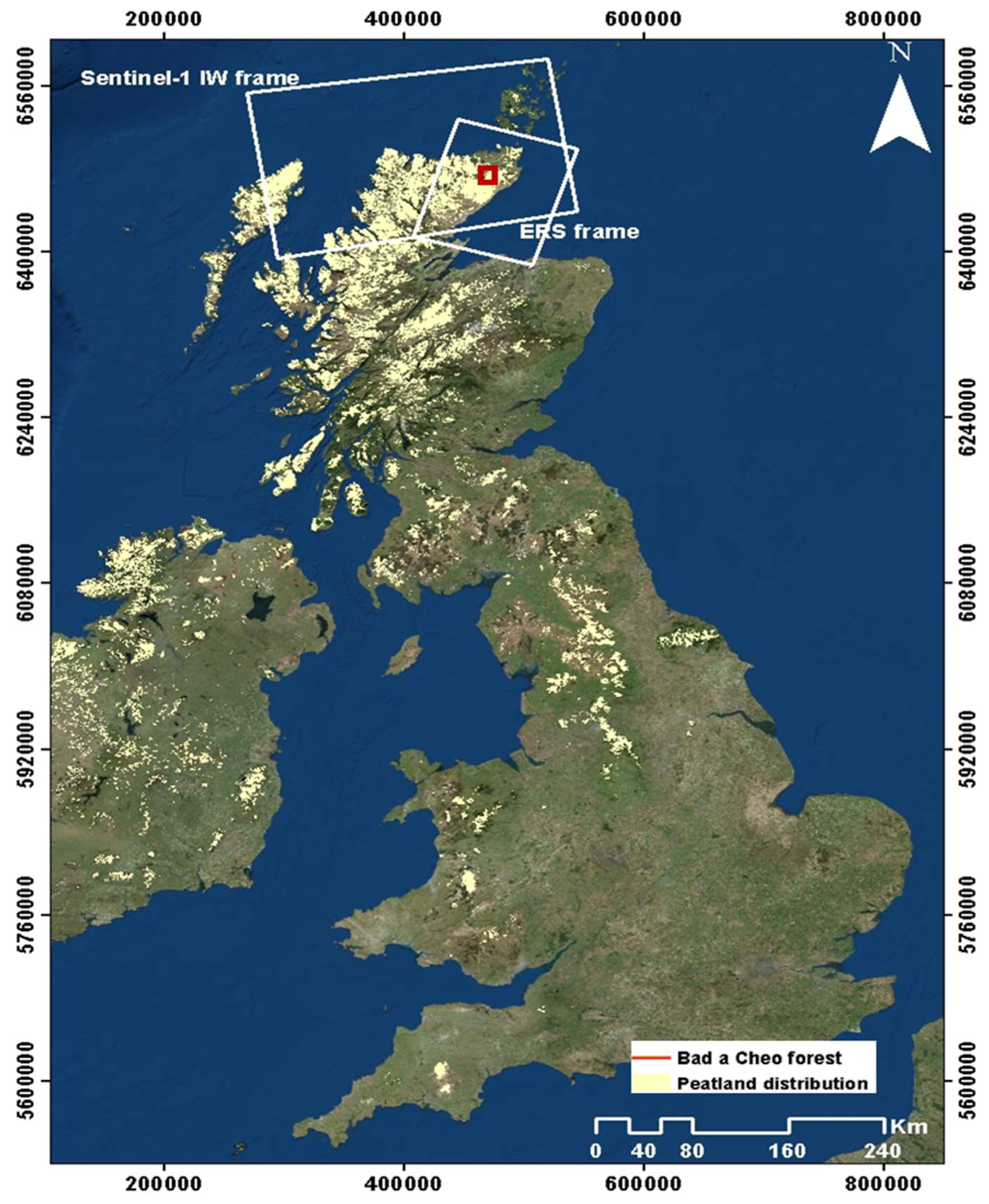
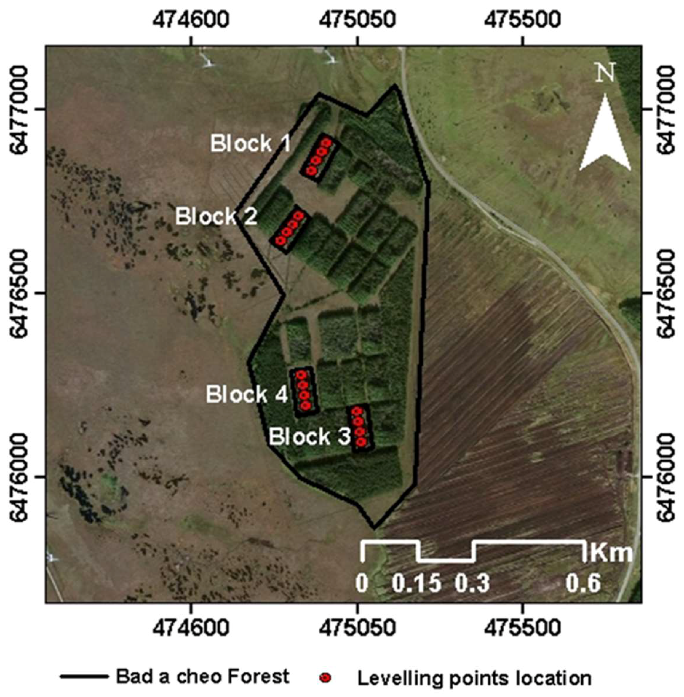
2.1. Site Selection

The Flow Country of Caithness and Sutherland, Northern Scotland, UK is the largest expanse of blanket bog in Europe, covering about 4000 square kilometres (Figure 1a). Peatlands in the UK have developed under peat forming vegetation, and, along with contemporary land management, this has resulted in a myriad of land cover classes and peat depths (and status) across the area [49]. The peat in some areas of the Flow Country was damaged between 1979 and 1987 through the planting of non-native conifer forests and the cutting of thousands of miles of drains. This has now been stopped and the area is under restoration. Indeed, the restoration of 21,000 ha per year of Scottish peatlands is one of the key interventions planned to achieve the 2050 target of 80% emissions reduction within the Climate Change Act (Scotland) 2009 to meet Kyoto Protocol commitments [50]. In the central eastern part of the Flow Country is the UK Forestry Commission’s Research Reserve at Bad a Cheo (475066 E, 6476417 N (WGS-1984-UTM-Zone-30N)), a site situated on wet, infertile blanket bog about 90 m above sea level, with mean annual precipitation of 930 mm [14,16] and featuring afforested plots. The area contains plots afforested in 1968, plots afforested in 1989, a few plots drained in 1989 but otherwise undisturbed and some areas that have been neither drained nor afforested. This reserve was used for the focused quantitative analysis of the ISBAS outputs, with the remaining 4000 km2 of peatland analysed contextually, providing qualitative analyses of the outputs from the processing of the SAR data.

2.2. Data

As determined by data availability over the study area, remotely sensed data from two SAR satellite systems were used in this study; this allowed for a different set of measurement scenarios to be investigated, principally related to the monitoring periods and temporal and orbital baseline constraints [45]. As determined by availability, dataset one was comprised of fifty-one ERS 1/2 C-band VV polarised SAR images from a descending orbit acquired for a long monitoring period between May 1992 and December 2000 (Table A1). All images were from frame 495, which covered the Flow Country AOI and were in single look complex (SLC) format suitable for a DInSAR analysis (Figure 1b). Dataset two (again determined by availability) was comprised of forty-seven Sentinel-1 Interferometric Wide (IW) SLC images (Figure 1b) acquired from satellite A in an ascending orbit over a much shorter monitoring period between March 2015 to December 2016 (Table A2). All IW images were downloaded from the Sentinel-1 scientific data hub (ESA, 2014c) and only the VV polarization mode data were used in the processing. Both datasets were separately processed using the ISBAS DInSAR technique [39,41] to calculate annual surface motion velocities (m/year) and their standard errors during the respective monitoring periods across the Flow Country.
Field data on surface motion had been collected at the UK Forestry Commission’s Bad a Cheo Research Area [14,16] by repeated optical levelling (Anderson et al., in prep). Although temporally concurrent to the SAR data, these field surface motion data were not collected for the purpose of comparison with the InSAR surface motion outputs; however, we use them here in the absence of any other field data on surface motion of the Flow Country. From 1989 to 1994, we repeated the levelling twice per year, once in spring and once in autumn. Then, for 1994–1999, we reduced the frequency to once per year, in the autumn. The next repetition was in spring 2005. Four blocks of a randomised block afforestation experiment had been surveyed here between 1989 and August 2016 (after which the reserve was clear-felled and no further measurements taken) (Figure 2), which more or less covers the same time period as the ERS and Sentinel-1 observations. Each block contains four 42 × 20 m plots; in each case, one of the plots is drained but unplanted and the other three are drained, ploughed and planted. Observations of peat height were made along a longitudinal mid-line transect of each plot with measurements at a fixed set of 85 locations related to the ploughing pattern, including drain bases, bases of furrows, tops of ridges and the original surface mid-way between ridges and beside them. In the drained but unplanted plots, 42 measurements were made including drain bases and the original surface at 1 m intervals along the transects. A local benchmark had been established beside each block in 1988 by pushing a metal rod vertically through the peat and hammering it into the mineral substratum [16]. These benchmarks by each of the four blocks were installed to act as local benchmarks against which to detect changes in the ground surface level due to peat consolidation, shrinkage, compression and oxidation and tree root growth. These were sufficiently well anchored in the mineral substrate to be used for this purpose and our assumption is that (though no measurement made to verify this) any vertical motion of the mineral substrate is negligible compared to vertical motion of the ground surface due to processes in the peat. Before and after surveying the points on each transect, which were all done from a single tripod position, the appropriate local benchmark was surveyed from the same tripod position so that heights on the transect could be expressed as heights relative to these. These measurements of the local datum were also a check to confirm that the automatic level had not inadvertently moved during the transect survey, which it never had. The observations of the heights were surveyed with a Topcon AT-F6 automatic level and rounded to the nearest 1 cm [16]. The mean height change of each transect was then used for comparison with the ERS and Sentinel-1 derived surface motion data sets, estimated by fitting a linear trend through the plot mean levelling heights. Twelve measurements for each levelling transect from 1991 to 2001 were used with the ERS data set (28/04/92–04/12/2000); however, due to the timing of this study, only two measurements were available to compare with the Sentinel-1 data set (28/01/15–03/08/2016). Qualitative comparisons to site condition were made on several sites across the Flow Country as a whole, on the basis of land cover and use (e.g., drained, forested, clear felled, presence of pool systems, bare peat, mineral soil), as delineated via visual interpretation of optical satellite images available from the Google Earth geobrowser [51].

3. Methods

3.1. Data Processing of SAR Data Using ISBAS

All ERS and Sentinel-1 images were processed using the ISBAS DInSAR technique [40,44], using temporal and orbital baseline constraints that allow for the maximisation of spatial coherence and a reduction of the contribution of DEM errors in the generation of the differential interferograms [52]. In order to increase the quality of the phase estimation and reduce the noise of the radar signal in the scene, the interferograms were multi-looked using a window size of 4 × 20 (range × azimuth) pixels for the ERS data and 22 × 5 pixels for the Sentinel-1 data, giving a final pixel dimension of approximately 100 × 100 m in ground range for ERS and 80 × 70 m for Sentinel-1. In both cases, the points that are derived from ISBAS processing are considered coherent when the average coherence is greater than or equal to 0.25, in accordance with the SBAS technique [41,53].
ISBAS processing was then performed only for coherent points as defined above. As reported in [46], areas with sustained coherence over all interferograms, such as in urban areas, have a low standard error; over areas for which coherence is more intermittent, such as in rural areas, the standard error increases. Therefore, care was taken to limit the minimum number of interferograms contributing to a coherent pixel to control the standard error. Differential interferograms were generated through calculating the phase difference between a pair of images and subtracting off a simulated phase calculated using the image geometry and a digital elevation model from the SRTM mission [53]. After generation of the differential interferograms, close attention by way of visual inspection was paid to identify any anomalies (i.e., atmospheric interference). No clear errors were observed or they had been removed through the processing that had been applied.
Phase unwrapping was implemented using a statistical cost network flow algorithm described by Chen and Zebker [54], to individually unwrap all the ISBAS points within each interferogram. Numerous previous studies using ISBAS have used one reference point and this was the case here. The same stable reference point, located in Dounreay on the Northern coast at 58°34′44″N 3°44′23″W, was used for both datasets’ image stacks. The selection of the reference point is extremely important because all the velocity results are relative to this point. Therefore, the reference point is expected to be stable, with zero velocity. The choice of the reference point was made subject to a statistical consideration relating to the coherence of the signal and the minimum standard deviation of the phase in all interferograms (i.e., the reference point has a high coherence and displays a low phase standard deviation across all interferograms). Dounreay is used since this is a stable high-coherence area and thus a low noise, zero-mean, neighbourhood. Through this choice of location of the reference point, any chance of erroneously choosing an unstable point has been minimized and the phase can thus be easily unwrapped and related to other stable areas surrounding it. Note that the resultant reference point is very close to a Thurso (THUS) Global Navigation Satellite System (GNSS) station (less than 1 km distance between them), see Figure 3.
All ISBAS velocity results are in the line of sight (LOS) direction, towards or away from the satellite. In order to enable an equivalent comparison between LOS velocity (VelLOS) results with the field acquired levelling data, all of the velocity results were converted to an equivalent vertical (Velvert) velocity by:
Velvert = VelLOS/cosθ,
where θ is the incidence angle from the surface normal. Here, the incidence angle was explicitly calculated for each coherent point using the satellite and image geometry. It should be noted that the correction that was applied assumes that the ground displacement is wholly in the vertical direction only, which is a reasonable assumption given that analyses of the data from the THUS Global Navigation Satellite System (GNSS) station in Thurso reports a vertical velocity for the period 2007 and 2014 was 0.6 ± 0.5 mm/year using ITRF 2008 reference frame [55]. The vertical velocity for the reference point as measured by the ISBAS technique was −0.17 ± 0.34 mm/year. Given that the geology is the same across the study, this stability should be case for the Bad a Cheo reserve too. However, in cases where horizontal motion is anticipated, it is possible to resolve the vertical and lateral components of motion using a stereo analysis of separate results from ascending and descending orbits, as demonstrated by Lanari et al. [56]. It is useful to note here that all pixel values in a multilooked, unfiltered interferogram are independent of each other and therefore errors in one pixel have no connection to the errors of its neighbours. Phase unwrapping merely adds an integer number of cycles to a pixel value and therefore does not propagate random errors or biases in any individual measurements. A ‘stable’ reference point simply means that its motion is so small that it does not require phase unwrapping (i.e., there are no integer cycle errors). As long as this condition is met, none of its intrinsic motion or noise will be propagated to any other pixels in the unwrapped phase. Note that the GNSS station observations are only used to confirm that the pixel location is stable—at no point is the pixel value adjusted to agree with the GNSS velocity.

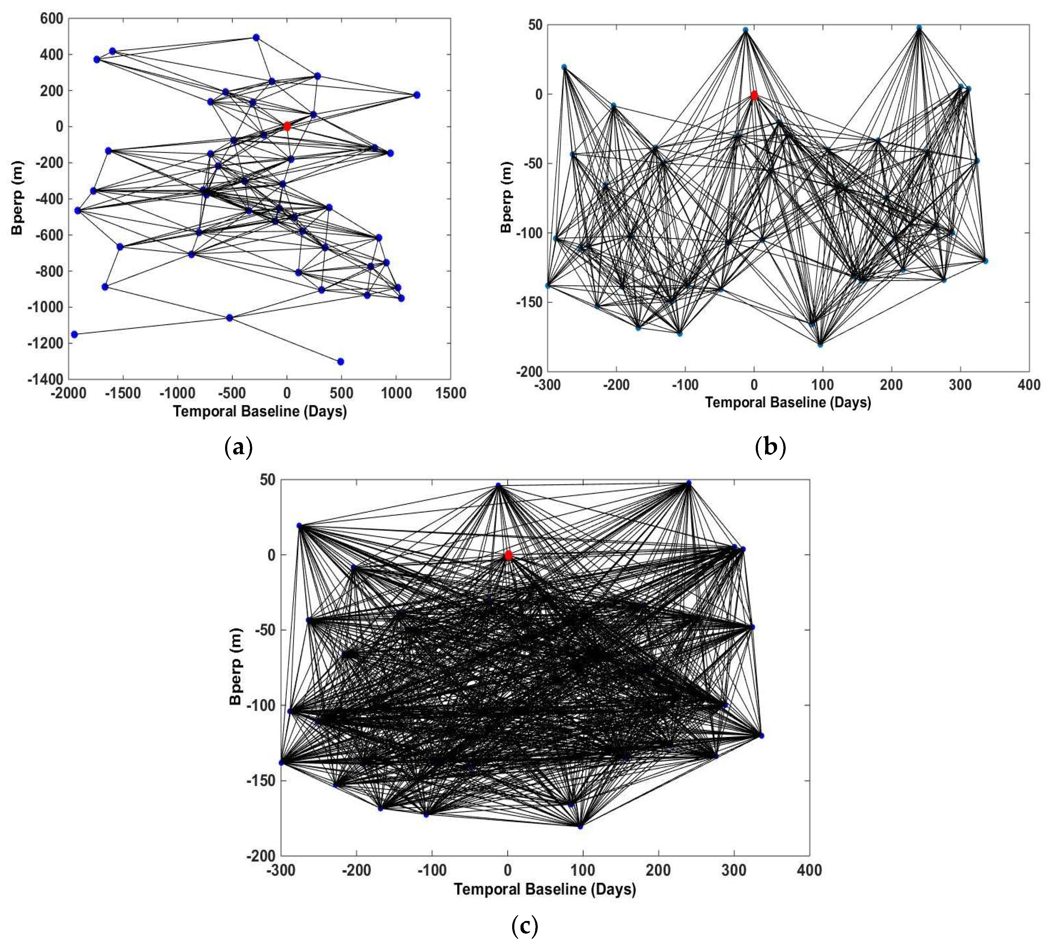
3.1.1. ERS ISBAS Processing

The fifty-one ERS C-band VV polarised SAR images were processed using constraints of a maximum 250 m perpendicular baseline and four-year temporal baseline between any interferometric pair used. This follows previous studies [41,45,53] and ensured limited spatial decorrelation and topographic errors and that interforemetretic coherence was preserved. The resultant interferograms (pairs) are depicted in Figure 4a; the total number of generated interferograms was 249, corresponding approximately to over 19% of the possible pair combinations of the ERS data set. However, a threshold value of 72 interferograms was used as the minimum point threshold. The point threshold is an indication of the minimum number of coherent interferograms that contribute to the analysis of each pixel. As indicated in Cigna and Sowter [45], a high point threshold indicates a low standard error, which is a preferred outcome, but at the cost of poor coverage. For example, if the point threshold is at a maximum, equal to the number of interferograms, the coverage is very close to that of a standard SBAS or PSI survey with most points over hard targets such as buildings or infrastructure and very few points over vegetated peatland areas. Therefore, the approach here was to successively lower the point threshold from its maximum value until an acceptable coverage was reached, but with an acceptable compromise to the standard error. This rule allows the ISBAS algorithm to accept points that may not be high quality in all interferograms (N) (i.e., intermittent coherence pixels), which is a characteristic of vegetated sites such as peatlands.

3.1.2. Sentinel-1 ISBAS Processing

The forty-seven Sentinel-1 Interferometric Wide (IW) SLC images were processed with a maximum normal perpendicular baseline of 200 m. With this perpendicular baseline, two different temporal baselines were used: six months and approximately two years (i.e., the entire period of the observations). The longer baseline was determined by the Sentinel-1 record at the time of data analyses. The shorter baseline of six months was chosen to examine if this had any impact on potential phase ambiguity, particularly in this dynamic peatland environment. With the six-month temporal baseline, 493 differential interferograms were formed, which corresponds to 45% of the possible pair combinations (Figure 4b); with the two-year temporal baseline, the number of resultant differential interferograms was 1071 (Figure 4c), corresponding to over 99% of the possible pair combinations. The point threshold values for the six-month and two-year temporal baselines were 246 and 420 interferograms, respectively. Further details of the ISBAS processing of Sentinel-1 data can be found in [44,46].

3.2. Data Analysis

The resultant vertical velocity maps produced from the processed ERS and Sentinel-1 data were evaluated both qualitatively (i.e., through comparisons with known peat subsidence and accumulation patterns over the study area, mainly related to land cover and site history) and quantitatively (i.e., through comparison with the field levelling data). Prior to evaluation, the vertical velocity outputs from the ERS and Sentinel-1 ISBAS processing were output as raster layers and orthorectified using nearest neighbour interpolation to provide pixels at a uniform 50 m spacing in a UTM map projection.
The fortuitous nature of the availability of the levelling data meant that only general patterns in surface motion were extracted and compared with the InSAR outputs. Although a useful ground dataset, it could not be used for a validation exercise per se—a key issue was that the output spatial resolution of the ISBAS velocity maps is clearly much larger than the individual field levelling transect means (four transect means per block—see Figure 2). As a result, all levelling points from each block and all raster cells of the ERS or Sentinel-1 outputs within each block were extracted for the simultaneous time period and used for further analyses. Moreover, the surface motion outputs for all the raster cells in the reserve as a whole were also extracted. It should be noted that this meant that the measurements for each of the four blocks are from both peatland that had forests for the entire study period but also peatland that had been drained at the same time but not planted. Analysis was undertaken through comparison between the levelling data and the InSAR velocity maps and this took two forms. The first was to plot the mean and standard error of the ground motion graphically for each of the four blocks separately, for each of the four blocks as a whole (i.e., all together) and also for the reserve as a whole. The second was to conduct a Wilcoxon–Mann–Whitney U-test at the scale of the blocks. This non-parametric method tests compare the arithmetic means of two samples (i.e., levelling data and InSAR data) are different or not. For clarity, we should stress that in this comparison the levelling measurements are relative to the relevant separate benchmarks and the InSAR measurements relative to the reference point at Thurso.

4. Results

For both the ERS and Sentinel-1 datasets, the spatial coverage of vertical velocity maps over the peatland area of the Flow Country attained a significant proportion of total coverage (over land). A measure of the coverage provided by the ISBAS method over this predominantly rural area is the solution density: the ratio between the number of pixels providing a solution and the total number of processed pixels over land [44]. On the ERS ISBAS velocity map, ISBAS points cover more than 70% of the total land area; on the Sentinel-1 velocity map, they cover 87% of the area (Figure 5, Figure 6 and Figure 7). The ERS derived vertical velocity maps and histograms (Figure 5) illustrate the spatial and statistical distribution of velocities and their standard errors for the time period 1992 to 2000. Negative LOS velocities indicate subsidence, whilst positive values indicate uplift. The mean vertical velocity of all ERS ISBAS points across the entire scene was −0.0006 ± 0.0012 m/year, with values ranging from −0.0081 ± 0.0024 m/year to 0.0071 ± 0.0015 m/year. Over the open peatland areas the standard error is very low due to the large number of coherent pixels per point. Over agricultural and forested areas, the standard error increases due to the intermittent coherence.
Sentinel-1 derived vertical velocity maps and histograms (Figure 6 and Figure 7) illustrate the spatial and statistical distribution of velocities and their standard errors calculated using temporal baselines of six months (Figure 6) and two years (Figure 7) for the time period 2015 to 2016. These velocity maps overlap with those obtained with the ERS data apart from a transect that dissects the study area along the track direction. This was due to the swaths that made up the IW images not overlapping in all images. Notwithstanding this missing data, the six-month temporal baseline generated a mean vertical velocity of −0.0072 ± 0.003 m/year for the entire scene with values ranging from −0.048 ± 0.005 m/year to 0.019 ± 0.004 m/year. The two-year temporal baseline generated a mean vertical velocity of −0.0048 ± 0.002 m/year with values ranging from −0.0223 ± 0.0017 m/year to 0.008 ± 0.0014 m/year. As was evident with the ERS data, the standard error of the Sentinel-1 velocities also increases over agricultural and forested areas due to intermittent coherence.

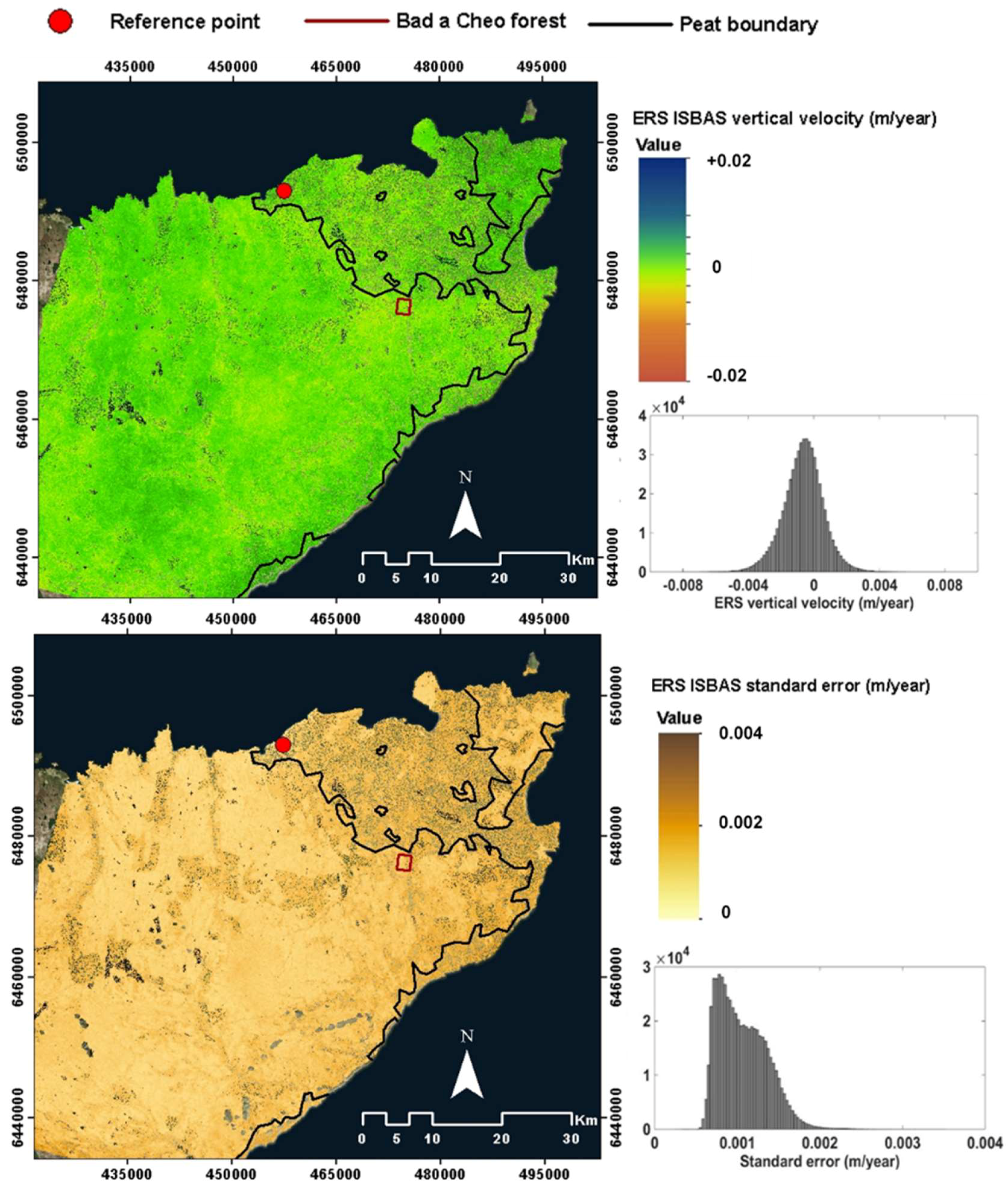
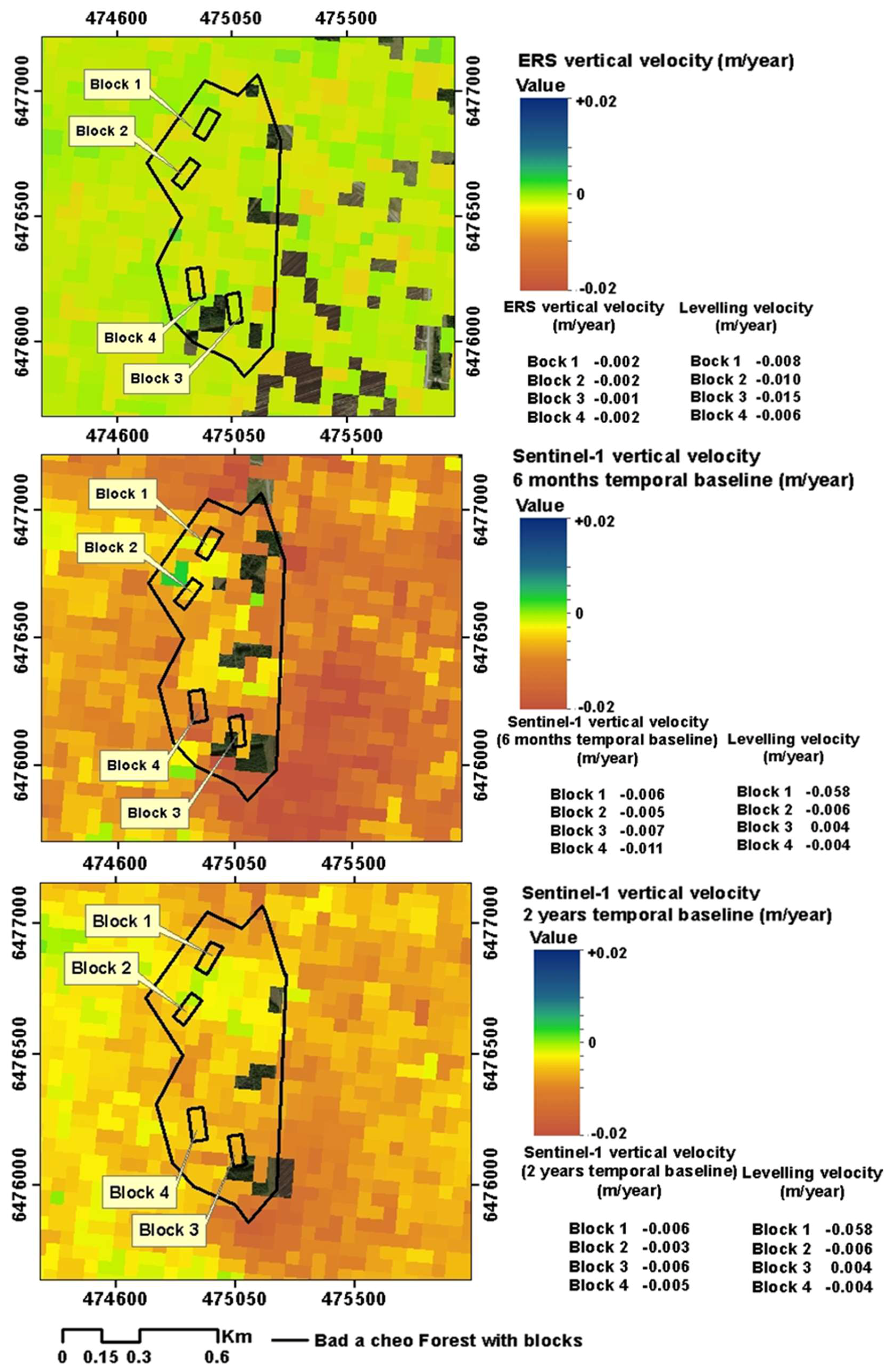
4.1. Qualitative Analysis

At the scale of the whole scene, qualitative analysis indicates that the highest rates of subsidence occur at the margins of the peatlands where the peatland intercalates with agricultural land. This is most obvious along the eastern margin of the Flow Country, which is also the area that receives the lowest precipitation [57]. High values of subsidence are also associated with plantation forestry and, in upland areas, with bare peat. Four areas of interest are highlighted to illustrate the qualitative relationships to land cover/use at higher spatial resolution (Figure 8). These areas show that peatland pool systems are clearly associated with areas of stability or uplift, as are areas of peatland far from lines of drainage. Plantation forest and clear felled forest are clearly associated with subsidence, although, within forested areas, this relationship is not uniform. The main effect of the plantations is to reduce the water content of the underlying peat and thus causes subsidence. The Flow Country extract indicates that the northeast is dominated by subsidence rates of more than 0.005 m/year and this is a forested area. The one stable area of the scene to the southwest is that showing healthy peat as indicated by the pool systems. The Bowside Lodge extract is a classic peatland area—dominated by stability or slight uplift—with minimal drainage and pool systems evident; the one area of high subsidence rates through the centre-left of the scene intersects with forestry. The Loch Sletill extract is one dominated by subsidence and features bare peat, forest and clear felled forest (in the southwest). Lastly the south Westerdale scene is mixed in terms of surface motion. Those areas dominated by stability or uplift (central area and to the southeast) are far from lines of drainage and/or feature a peatland pool system. These described observations between surface motion and land cover/use align entirely with the expected peatland condition of the Flow Country as a landscape and indicate that the InSAR data provides a meaningful qualitative and relative indicator of peatland condition. Further and robust utility of these data would be provided if the velocities obtained had absolute meaning.

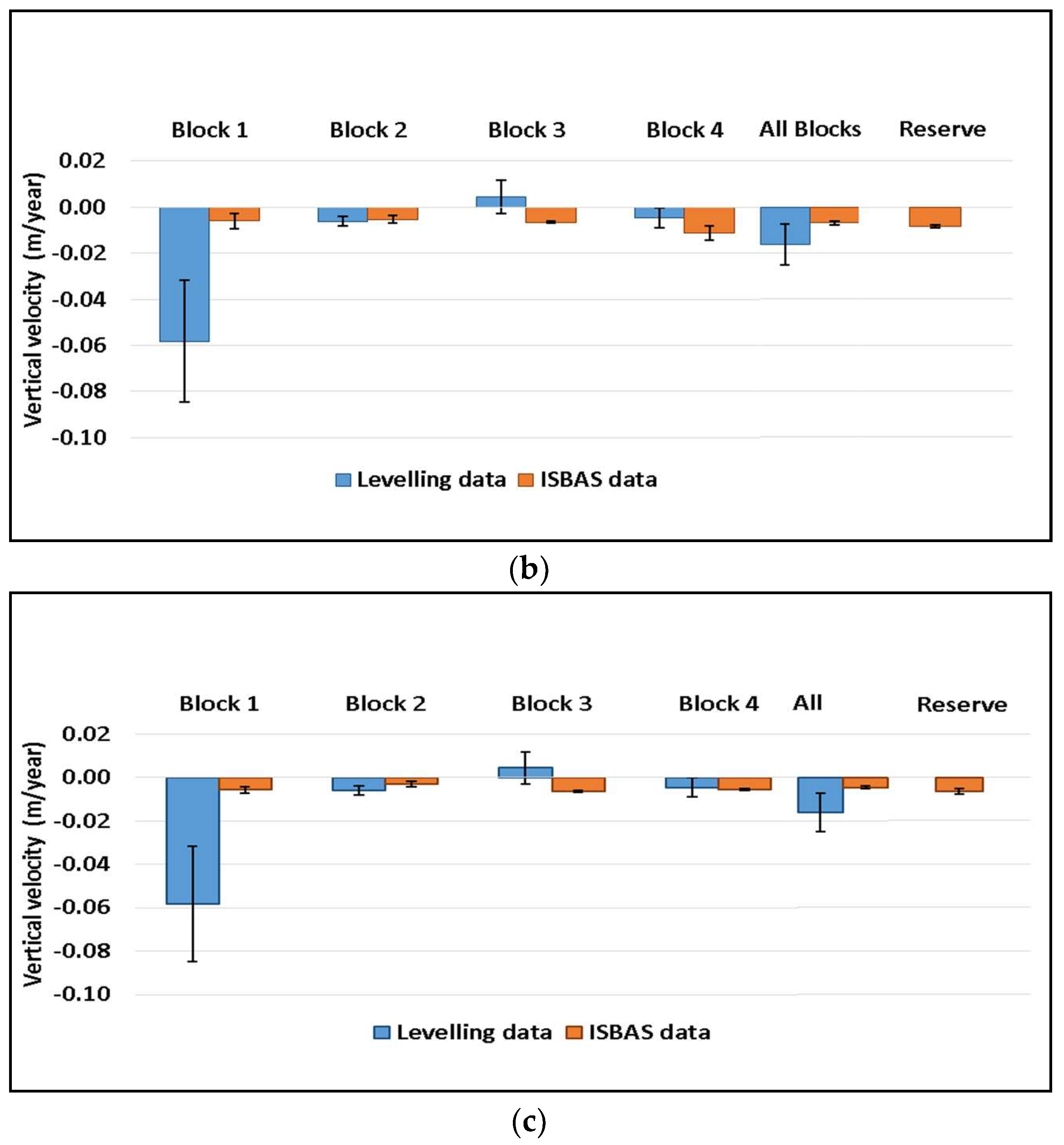
4.2. Quantitative Analyses

At the scale of the whole Bad a Cheo Forest Reserve, the overall trend of motion as captured by the InSAR data was of subsidence; this was the case for the both ERS and Sentinel-1 data (for both six-month and two-year temporal baselines) (Figure 9). The ERS satellite measured a mean rate of subsidence across the period of 1992 to 2000 was −0.0019 m/year with an associated standard error of 0.0001 m/year. For Sentinel-1 ISBAS using six-months and two-year temporal baselines, the mean rates of subsidence across the period March 2015 to December 2016 were −0.009 m/year and −0.006 m/year respectively. The associated mean standard error was 0.001 m/year, respectively. At the scale of the four blocks as a whole within the Reserve, the overall trend of motion as captured by the InSAR was of subsidence; this was the case for the both ERS and Sentinel-1 data for both temporal baselines used across the time period under investigation (Figure 9). The mean rate of subsidence for the blocks as a whole for ERS ISBAS points was −0.002 m/year and the associated mean standard error was 0.0004 m/year. The Mann–Whitney U-test analyses comparing this ERS measure with that measured by the levelling (n1) illustrates that, while the ERS data (n2) correctly predicts the direction of ground motion (i.e., subsidence), its magnitude (Figure 10a and Figure 11a) is different to that measured by the levelling data (at the 95% level of confidence) (n1 = 16; n2 = 12). For the exact same time period, the mean of the levelling measurements was −0.01 m/year and its standard error 0.001 m/year. For the Sentinel-1 data, it was the case that the mean of the levelling measurement for the time period of comparison was −0.016 m/year and its standard error 0.009 m/year. Comparing this (n1) with the Sentinel-1 ISBAS (n2) mean and SE using the Mann–Whitney U test reveals that for both the six-month and two-year temporal baseline, there was no difference at 95% level of confidence in the measurements. The Sentinel-1 data (using a six-month baseline) had a mean rate of movement of −0.007 m/year with a standard error of 0.001 m/year and the Sentinel-1 (using a 2 year baseline) had a mean rate of movement of −0.005 m/year with a standard error of 0.001 m/year.
By looking at Figure 10 and Figure 11, it is evident that, although the general trend of the Reserve measured by both the InSAR ISBAS and the levelling methods is that of subsidence, there is spatial variability within the Reserve with some of the ISBAS output points showing uplift, and the pattern of variability differs between that captured by the ERS and Sentinel-1 satellites. Taking each Block individually, it is the case that the levelling data shows an approximately linear trend of motion in all four blocks (Figure 10a,b); however, the variability of the velocity is greater than the variability in velocity measured with the InSAR ISBAS data. As a case in point, during the two-year period covered by the Sentinel-1 data, the average of the levelling measurements per block indicate that three blocks were subsiding (block 1 with 0.04 m/year, block 2 with 0.004 m/year and block 4 with 0.003 m/year) and one block (block 3) experienced uplift of about 0.003 m/year (Figure 10b). Although caution is required here as levelling measurements were only made on two occasions and also the final measurement made was prior to the end date of the Sentinel-1 acquisitions, it is the case that comparison with the Sentinel-1 measurements (Figure 10b and Figure 11b,c) indicates a mismatch with block 3, with both temporal baseline outputs showing subsidence, albeit at small rates, rather than uplift during this period.

5. Discussion

The ISBAS maps of surface motion output in this paper represent the first contiguous maps of peatland surface motion over the Flow Country of Scotland, UK. Using knowledge of peatland surface motion as provided by ground data, i.e., through expert interpretation of the land cover shown on high spatial resolution optical satellite data and best available levelling measurements, the real potential of using satellite InSAR data processed using the ISBAS method has been demonstrated. This is much needed mapping given the links between peatland condition and ecosystem services and, although we cannot fully explain from this work the exact magnitudes in the differences and uncertainties, the results presented here indicate that further investigation of this methodology should be undertaken. Full validation of this remote sensing method for this application is required, particularly given that the levelling measurements were not designed for the validation of such mapping. Further work could pay dividends and would build upon previous studies that have only alluded to the possibility of peatland surface motion being measured by InSAR/ISBAS but had much less evidence from ground observations to support conclusions e.g., [43,45,58]. This study over temperate peatland is also a useful addition to the literature on INSAR for peatlands. All previous, albeit few InSAR studies undertaken to date have been in very different peatland environments to that of the Flow Country. Moreover, these studies have used different SAR data and processing techniques. Subsidence of up to 7.65 cm/year was reported in Central Kalimantan, Indonesia using the SBAS technique applied to ALOS L-band data [59] and up to 1 cm/year in the Zennare basin in Venice Lagoon Italy using ERS data in Interferometric Point Target Analysis (IPTA).
Qualitatively, the results obtained seem to present a meaningful account of peatland condition in terms of its growth, stability or subsidence across the entire region that would appear to match expectations in areas where the conditions are either known or can be reasonably anticipated. The overall trend of peat surface subsidence for the Flow Country revealed by the InSAR outputs concurs with expectations, based on the fact that much of the area of the peatland is drained, afforested or eroding. It is reasonable to assume that, in the case of drained or eroding ground, there are net greenhouse gas emissions. This assumption cannot be made for afforested ground, which is thought to be a net source initially due to peat disturbance and drainage, becoming a net sink as tree growth sequesters carbon and revert to a net source after 50–200 years as carbon dioxide release from the breakdown of timber products starts to exceed sequestration by the trees [17]. On this basis, the values of the InSAR outputs are considerable in their landscape spatial resolution and this should enable identification of areas undergoing change and more effective monitoring, management and intervention. Thus, the results obtained are encouraging and suggest that, in this era of BigInSAR [45], this study is timely; it indicates the value in using InSAR data to support a monitoring system of peatland at all spatial scales [27]. The need for the increase in InSAR data via higher temporal resolution afforded by constellations is demonstrated by the ERS results here, which were compromised by the gaps in the time series—this meant using a four-year temporal baseline, resulting in the measurement of small deformation rates in comparison with what the Sentinel-1 data measured (due to ambiguity). Regular acquisitions of Sentinel 1 with short repeat cycle of each 12 days made it possible to decrease the temporal baseline and measure greater rates of deformation.
As already stated, there is, however, further work to be conducted to fully understand the value of the InSAR ISBAS outputs, particularly given that the quantitative accuracy of the ISBAS method over peatland is hard to fully establish on the basis of this study. The results of the quantitative analyses come with the caveat that recognises that the levelling data were not collected for the purpose of comparison with the satellite-derived measurement of surface motion. Hence, results are to be treated with some caution, with only general patterns noted. In both the levelling and InSAR measurements, there will be some degree of error propagation that will need to be fully quantified in future studies. For example, an error analysis on the levelling data reveals sources of error during transect reading (e.g., telescope instability, curvature, and rounding error) that could be up to ±18 mm and further that, during local datum level reading, another ±18 mm of error could be introduced. This combined with an estimated error of −0.17 mm/year due to a different reference point being used for the InSAR (i.e., the InSAR vertical velocity at the reference point) and levelling measurements indicate the need for further work, particularly focused on the quantitative validation of the InSAR vertical velocity outputs.
For future validation studies, several issues need to be considered. One issue concerns the temporal mismatch between the levelling measurements and the Sentinel-1 data. There is a need to understand magnitude of short term seasonal or inter-seasonal oscillations relative to long-term trends to determine the sensitivity of InSAR measures to start and end point selection. It is likely, therefore, that the Sentinel-1 comparison could have been biased by any seasonal signal, particularly over the short period of analyses. This could explain the higher vertical motion rates for the Sentinel in comparison to that for the ERS outputs. Unfortunately, we were constrained by the periods for which the levelling results were collected (and the project in the Bad a Cheo reserve ended) so could not extend this time period. Another issue is that the levelling transect, which is typical of peatland studies, lacked the systematic spatial coverage to adequately validate the InSAR. Nevertheless, this has been useful in building upon the qualitative comparisons in demonstrating that forested areas on peatland have an overall trend of subsidence. At the scale of the reserve as a whole, both the levelling measurements and the InSAR ISBAS outputs for both ERS and Sentinel-1 (six-month and two-year temporal baseline) satellites agree that the peatlands of the Bad a Cheo reserve are subsiding. Given that the peatland in this particular area is covered with trees, which lowers water tables and makes the peat compact, this is encouraging. Furthermore, spatial variations seen in the InSAR ISBAS outputs may be explained by the fact that earlier levelling work at the Bad a Cheo Reserve has shown high spatial variability in surface level change related to the layout of the forest plots and other unknown causes [14]. Within the forest plots, variability in surface level change relates to the tree species or species mixture, the different surfaces of the ploughing micro-relief and to the deep drains and associated spoil ridges.
Nonetheless, the accuracy of the InSAR measurements shows differences and uncertainties when compared with the levelling measurements. This could be a result of question around the suitability of levelling measurements made along transects at 42 × 20 m resolution to compare against a pixel size of approximately 100 m × 100 m. Any further validation campaign should adopt calibration and validation methods designed for measuring contiguous mapping (i.e., be randomly located) and consider intra-pixel deployment of levelling measurements. That said, however, peatland is predominantly water (typically about 95% in volume) and surface motion both short and long term is predominantly driven by changes in the mass of water within the peat body (e.g., [60]). Hydraulic continuity operates on scales of much greater than 100 m, the scale of mire units (mesotopes) and mire complexes (macrotopes) [61]. As the mass of water within the peat increases the pressure increases and the surface expands; as water is removed, the peat collapses. Long-term bog growth results from both the accumulation of both carbon (plant matter) and water. Given that hydraulic continuity operates on scales greater than 100 m, it could therefore be a reasonable assumption that independent measures of surface motion should display the same trends and rates over long periods of time.
Notwithstanding these known shortcomings of the levelling measurements, they are indicative of the range of vertical movement that could be present at this site—up to −0.11 m/year. Within the Reserve, neither of the satellites measured motion to that extreme. This is due to the limitation imposed by the radar and the chosen temporal baseline relative to the actual rate of surface motion. The smoothing of displacements when averaging the information present in the SAR data by heavy multi-looking might also explain the findings. Phase unwrapping has the greatest influence on the quantitative measurement of deformation on an individual interferogram. Phase unwrapping is applied to determine the phase ambiguity that occurs whenever there is a fringe in an interferogram (i.e., when the phase jumps from + to − radians, or vice versa). When fringes are well-defined and there is no noise, this can be a simple task; however, when there is noise and coherent pixels are sparse, such as in vegetated areas, this can be very difficult and lead to an underestimation of fringes and, consequently, an underestimation of the deformation. This is the most likely reason for ISBAS underestimating the magnitude of peatland subsidence in the Reserve.
It is possible to improve the measurements of an InSAR survey by reducing the number of fringes in the interferogram and therefore reducing the likelihood of phase unwrapping problems. This would be achieved by simply reducing the time difference between pairs, if possible. For an ISBAS survey, we can attempt this by reducing the maximum temporal baseline possible. However, as made evident in Figure 4, this drastically reduces the number of pairs used for the survey and hence increases the standard error. There are other consequences in reducing the temporal baseline threshold, in that this also reduces the ability to detect smaller rates of deformation. There is clearly more work to be done on selecting a more appropriate temporal baseline for peatland studies, but to do so requires more ground observations to identify what rates to expect. Indeed, as made evident in this study, there are differences in the surface motion outputs from Sentinel 1 by virtue of the different temporal baselines used, with the six-month result showing a larger magnitude of velocities compared to the two-year result. Going forward, our ability to experiment with this parameter will be improved as more Sentinel-1 data is collected in the coming years, which will give us the opportunity to reduce baselines but still retain a high number of observations and doing so will provide more confidence in the surface velocity measurements made—the accuracy of a linear velocity rate is inversely proportional to the time span covered by the measurements. The outcome of this study has highlighted the need to do this. This study also highlights the need to consider the role of corner reflectors. For low coherence areas, such as peatland where the natural reflectors are unavailable, the lack of coherence can be avoided using artificial corner reflectors [62]. These devices can be installed in the AOI, which can provide a strong response in the SAR images and result in good interferometric phases to derive precise deformation estimates for the AOI. However, the ISBAS method used here is entirely different from a persistent scatterer method as each pixel is a summative representation of the motion within a 100 m × 100 m area on the ground, as opposed to the brightest point within it. Therefore, corner reflector methods which produce small bright measurements of only a single point within the resolution cell are not relevant for validation here unless it is certain that the point is representative of the entire cell. Again, further investigation is needed.

6. Conclusions

In this paper we have pointed to a potential satellite-based monitoring system based on C-band SAR images that could operate over peatlands. Specifically, we examined the feasibility of the ISBAS technique for monitoring long term surface motion over peatland areas of the Flow Country, in the North East of Scotland. We conclude that, notwithstanding the shortcomings noted herein and the assumptions made (i.e., there is no horizontal motion in the are—this underpins the conversion from LoS to vertical velocity in the ISBAS method), there is a real potential for using this method and remotely sensed data. There is now a real possibility of observing the entire landscape of the Flow Country peatlands with certainties in measurements that afford the direction of surface motion to be mapped across the area. Further work is required as outlined in the discussion and we conclude the need for a rigorous validation system that will allow one to understand how/if errors propagate through the use of the ISBAS method to process InSAR for peatland monitoring. Such understanding should assist in informing how a synergistic monitoring system between satellite and strategically deployed ground based observations (in locations where ambiguity and/or temporal decorrelation would limit the confidence in the measurements made) fit for validating the InSAR ground motion measurements could operate. Lessons learned from other EO validation campaigns will be invaluable here [63].

Author Contributions

All authors conceived of this work. L.A. and A.S. processed the InSAR data and R.A. acquired and processed the levelling data. D.S.B. and L.A. wrote the paper with editorial inputs from all authors. L.A. is a student of D.S.B. and S.M.

Funding

This work was supported by the Natural Environment Research Council [grant number NE/P014100/1].

Acknowledgments

As well as the UK’s NERC, the authors would like to acknowledge the European Space Agency (ESA) for the provision of ERS1/2 data via the Category_1 project ID: 32049: Monitoring the eroding extent of peatland surface over the Flow Country, Scotland by using ISBAS DInSAR technique, and Sentinel-1 data via Scientific Data Hub (ESA 2014c) and the Forestry Commission Bad a’ Cheo Research Reserve for the provision of the levelling measurements. The authors would like also to acknowledge the financial support of the Higher Education and Scientific Research Ministry in Iraq for the PhD scholarship of the first author. Finally, we would like to thank the reviewers for their constructive comments.

Conflicts of Interest

The authors declare no conflict of interest.

Appendix A

Table A1. ERS images dates and perpendicular baseline B relative to the master image (01/09/1997).
SensorDate B Date B Date B
ERS1/2 SAR (master)01/09/1997019/02/1996192.991504/05/199867.58448
01/05/1992−1150.6724/03/1996−1059.9808/06/1998281.1085
05/06/1992−463.96729/04/1996−74.705413/07/1998−906.11
23/10/1992−354.53812/08/1996−301.13417/08/1998−671.416
27/11/1992373.775516/09/1996−466.29821/09/1998−448.835
05/02/1993−886.40821/10/1996134.423104/01/1999−1303.58
12/03/1993−132.30525/11/1996493.761406/09/1999−931.75
16/04/1993416.457930/12/1996−412.73811/10/1999−775.74
25/06/1993−667.16703/02/1997−47.107515/11/1999−116.601
09/04/1995−705.74310/03/1997−330.68820/12/1999−616.819
18/06/1995−585.93714/04/1997252.114228/02/2000−753.803
19/06/1995−676.69819/05/1997−521.96903/04/2000−145.465
24/07/1995−352.88523/06/1997−450.92712/06/2000−892.831
27/08/1995−359.63728/07/1997−318.95917/07/2000−951.859
28/08/1995−375.16406/10/1997−181.01704/12/2000174.1707
01/10/1995−151.30810/11/1997−500.615
02/10/1995136.210215/12/1997−807.807
11/12/1995−217.74419/01/1998−578.707
Table A2. Sentinel-1A images dates and perpendicular baseline B relative to the master image (06/01/2016).
SensorDate B Date B Date B
Sentinel-1 SAR (master)06/01/2016011/02/2016−20.193417/05/2016−68.1864
12/03/2015−137.86320/09/2015−172.33404/07/2016−33.4788
24/03/2015−103.95602/10/2015−137.91716/07/2016−74.9726
05/04/201519.4311219/11/2015−140.41328/07/2016−103.857
17/04/2015−43.185301/12/2015−106.56109/08/2016−126.395
29/04/2015−110.73313/12/2015−30.401521/08/2016−93.4495
11/05/2015−109.98925/12/201546.0093802/09/201647.7846
23/05/2015−152.89118/01/2016−105.13814/09/2016−41.6521
04/06/2015−66.001330/01/2016−55.194726/09/2016−95.1289
16/06/2015−8.5010223/02/2016−29.21508/10/2016−134.011
28/06/2015−138.54930/03/2016−165.67320/10/2016−99.668
10/07/2015−102.08911/04/2016−180.5401/11/20165.327293
22/07/2015−168.3523/04/2016−40.09513/11/20163.495892
15/08/2015−38.704905/05/2016−67.143325/11/2016−47.841
27/08/2015−49.718629/05/2016−130.99107/12/2016−120.063
08/09/2015−149.4910/06/2016−134.575

References

  1. Zanello, F.; Teatini, P.; Putti, M.; Gambolati, G. Long term peatland subsidence: Experimental study and modeling scenarios in the Venice coastland. J. Geophys. Res. Earth Surf. 2011, 116. [Google Scholar] [CrossRef] [Green Version]
  2. Hooijer, A.; Page, S.; Jauhiainen, J.; Lee, W.; Lu, X.; Idris, A.; Anshari, G. Subsidence and carbon loss in drained tropical peatlands. Biogeosciences 2012, 9, 1053–1071. [Google Scholar] [CrossRef] [Green Version]
  3. Holden, J. Peatland hydrology and carbon release: Why small-scale process matters. Philos. Trans. A Math. Phys. Eng. Sci. 2005, 363, 2891–2913. [Google Scholar] [CrossRef] [PubMed]
  4. Yu, Z.; Loisel, J.; Brosseau, D.P.; Beilman, D.W.; Hunt, S.J. Global peatland dynamics since the last glacial maximum. Geophys. Res. Lett. 2010, 37. [Google Scholar] [CrossRef]
  5. Freeman, C.; Lock, M.A.; Reynolds, B. Climatic change and the release of immobilized nutrients from welsh riparian wetland soils. Ecol. Eng. 1993, 2, 367–373. [Google Scholar] [CrossRef]
  6. Kirschke, S.; Bousquet, P.; Ciais, P.; Saunois, M.; Canadell, J.G.; Dlugokencky, E.J.; Bergamaschi, P.; Bergmann, D.; Blake, D.R.; Bruhwiler, L.; et al. Three decades of global methane sources and sinks. Nat. Geosci. 2013, 6, 813–823. [Google Scholar] [CrossRef]
  7. Nykanen, H.; Alm, J.; Lang, K.; Silvola, J.; Martikainen, P.J. Emissions of CH4, N2O and CO2 from a virgin fen and a fen drained for grassland in finland. J. Biogeogr. 1995, 22, 351–357. [Google Scholar] [CrossRef]
  8. Smith, L.C.; MacDonald, G.M.; Velichko, A.A.; Beilman, D.W.; Borisova, O.K.; Frey, K.E.; Kremenetski, K.V.; Sheng, Y. Siberian peatlands a net carbon sink and global methane source since the early Holocene. Science 2004, 303, 353–356. [Google Scholar] [CrossRef] [PubMed]
  9. Crichton, K.A.; Anderson, K.; Bennie, J.J.; Milton, E.J. Characterizing peatland carbon balance estimates using freely available Landsat ETM+ data. Ecohydrology 2015, 8, 493–503. [Google Scholar] [CrossRef]
  10. Drew, S.; Waldron, S.; Gilvear, D.; Grieve, I.; Armstrong, A.; Bragg, O.; Brewis, F.; Cooper, M.; Dargie, T.; Duncan, C.; et al. The price of knowledge in the knowledge economy: Should development of peatland in the UK support a research levy? Land Use Policy 2013, 32, 50–60. [Google Scholar] [CrossRef]
  11. Lindsay, R.; Charman, D.J.; Everingham, F.; O’Reilly, R.M.; Palmer, M.A.; Rowell, T.A.; Stroud, D.A. The Flow Country: The Peatlands of Caithness and Sutherland; Joint Nature Conservation Committee: Peterborough, UK, 1988.
  12. Baird, A.J.; Belyea, L.R.; Morris, P.J. Upscaling of peatland-atmosphere fluxes of methane: Small-scale heterogeneity in process rates and the pitfalls of “bucket-and-slab” models. Geophys. Monogr. Ser. 2009, 184, 37–53. [Google Scholar]
  13. Bain, C.G.; Bonn, A.; Stoneman, R.; Chapman, S.; Coupar, A.; Evans, M.; Gearey, B.; Howat, M.; Joosten, H.; Keenleyside, C.; et al. IUCN UK Commission of Inquiry on Peatlands; Project Report; IUCN UK Peatland Programme: Edinburgh, UK, 2011. [Google Scholar]
  14. Shotbolt, L.; Anderson, A.; Townend, J. Changes to blanket bog adjoining forest plots at Bad a′ Cheo, Rumster Forest, Caithness. Forestry 1998, 71, 311–324. [Google Scholar] [CrossRef]
  15. Holden, J.; Gascoign, M.; Bosanko, N.R. Erosion and natural revegetation associated with surface land drains in upland peatlands. Earth Surf. Process. Landf. 2007, 32, 1547–1557. [Google Scholar] [CrossRef]
  16. Anderson, A.; Ray, D.; Pyatt, D. Physical and hydrological impacts of blanket bog afforestation at Bad a′ Cheo, Caithness: The first 5 years. Forestry 2000, 73, 467–478. [Google Scholar] [CrossRef]
  17. Cannell, M.G.R.; Dewar, R.C.; Pyatt, D.G. Conifer plantations on drained peatlands in Britain—A net gain or loss of carbon. Forestry 1993, 66, 353–369. [Google Scholar] [CrossRef]
  18. Gambolati, G.; Putti, M.; Teatini, P.; Camporese, M.; Ferraris, S.; Stori, G.G.; Nicoletti, V.; Silvestri, S.; Rizzetto, F.; Tosi, L. Peat land oxidation enhances subsidence in the Venice watershed. EOS Trans. Am. Geophys. Union 2005, 86, 217–220. [Google Scholar] [CrossRef]
  19. Ramchunder, S.J.; Brown, L.E.; Holden, J. Environmental effects of drainage, drain-blocking and prescribed vegetation burning in UK upland peatlands. Prog. Phys. Geogr. 2009, 33, 49–79. [Google Scholar] [CrossRef]
  20. Lindsay, R. The Great Flow—An International Responsibility; New Scientist Publications Expediting Inc.: Elmont, NY, USA, 1987. [Google Scholar]
  21. Parry, L.E.; Holden, J.; Chapman, P.J. Restoration of blanket peatlands. J. Environ. Manag. 2014, 133, 193–205. [Google Scholar] [CrossRef] [PubMed] [Green Version]
  22. Lees, K.J.; Quaife, T.; Artz, R.R.E.; Khomik, M.; Clark, J.M. Potential for using remote sensing to estimate carbon fluxes across northern peatlands—A review. Sci. Total Environ. 2018, 615, 857–874. [Google Scholar] [CrossRef] [PubMed]
  23. Novellino, A.; Cigna, F.; Sowter, A.; Ramondini, M.; Calcaterra, D. Exploitation of the intermittent SBAS (ISBAS) algorithm with cosmo-skymed data for landslide inventory mapping in north-western Sicily, Italy. Geomorphology 2017, 280, 153–166. [Google Scholar] [CrossRef]
  24. Tofani, V.; Del Ventisette, C.; Moretti, S.; Casagli, N. Integration of remote sensing techniques for intensity zonation within a landslide area: A case study in the northern Apennines, Italy. Remote Sens. 2014, 6, 907–924. [Google Scholar] [CrossRef]
  25. Massonnet, D.; Feigl, K.L. Radar interferometry and its application to changes in the Earth’s surface. Rev. Geophys. 1998, 36, 441–500. [Google Scholar] [CrossRef]
  26. Rosen, P.A.; Hensley, S.; Joughin, I.R.; Li, F.K.; Madsen, S.N.; Rodriguez, E.; Goldstein, R.M. Synthetic aperture radar interferometry. Proc. IEEE 2000, 88, 333–382. [Google Scholar] [CrossRef] [Green Version]
  27. Kim, J.-W.; Lu, Z.; Gutenberg, L.; Zhu, Z. Characterizing hydrologic changes of the Great Dismal Swamp using SAR/InSAR. Remote Sens. Environ. 2017, 198, 187–202. [Google Scholar] [CrossRef]
  28. Burgmann, R.; Hilley, G.; Ferretti, A.; Novali, F. Resolving vertical tectonics in the San Francisco bay area from permanent scatterer InSAR and GPS analysis. Geology 2006, 34, 221–224. [Google Scholar] [CrossRef]
  29. Colesanti, C.; Ferretti, A.; Prati, C.; Rocca, F. Monitoring landslides and tectonic motions with the permanent scatterers technique. Eng. Geol. 2003, 68, 3–14. [Google Scholar] [CrossRef]
  30. Canuti, P.; Casagli, N.; Farina, P.; Marks, F.; Ferretti, A.; Menduni, G. Land subsidence in the Arno River Basin studied through SAR Interferometry. In Proceedings of the Seventh International Symposium on Land Subsidence, Shanghai, China, 23–28 October 2005. [Google Scholar]
  31. Osmanoglu, B.; Dixon, T.H.; Wdowinski, S.; Cabral-Cano, E.; Jiang, Y. Mexico City subsidence observed with persistent scatterer InSAR. Int. J. Appl. Earth Observ. Geoinf. 2011, 13, 1–12. [Google Scholar] [CrossRef]
  32. Stramondo, S.; Bozzano, F.; Marra, F.; Wegmuller, U.; Cinti, F.R.; Moro, M.; Saroli, M. Subsidence induced by urbanisation in the city of Rome detected by advanced InSAR technique and geotechnical investigations. Remote Sens. Environ. 2008, 112, 3160–3172. [Google Scholar] [CrossRef]
  33. Cigna, F.; Del Ventisette, C.; Liguori, V.; Casagli, N. Advanced radar-interpretation of insar time series for mapping and characterization of geological processes. Nat. Hazards Earth Syst. Sci. 2011, 11, 865–881. [Google Scholar] [CrossRef] [Green Version]
  34. Cigna, F.; Del Ventisette, C.; Liguori, V.; Casagli, N. Insar Time-Series Analysis for Management and Mitigation of Geological Risk in Urban Area. In Proceedings of the 2010 IEEE International Geoscience and Remote Sensing Symposium, Honolulu, HI, USA, 25–30 July 2010; pp. 1924–1927. [Google Scholar]
  35. Hilley, G.E.; Burgmann, R.; Ferretti, A.; Novali, F.; Rocca, F. Dynamics of slow-moving landslides from permanent scatterer analysis. Science 2004, 304, 1952–1955. [Google Scholar] [CrossRef] [PubMed]
  36. Salvi, S.; Atzori, S.; Tolomei, C.; Allievi, J.; Ferretti, A.; Rocca, F.; Prati, C.; Stramondo, S.; Feuillet, N. Inflation rate of the colli albani volcanic complex retrieved by the permanent scatterers SAR interferometry technique. Geophys. Res. Lett. 2004, 31. [Google Scholar] [CrossRef]
  37. Tizzani, P.; Berardino, P.; Casu, F.; Euillades, P.; Manzo, M.; Ricciardi, G.P.; Zeni, G.; Lanari, R. Surface deformation of Long Valley caldera and mono basin, California, investigated with the ISBAS-InSAR approach. Remote Sens. Environ. 2007, 108, 277–289. [Google Scholar] [CrossRef]
  38. Teatini, P.; Strozzi, T.; Tosi, L.; Wegmüller, U.; Werner, C.; Carbognin, L. Assessing short- and long-time displacements in the Venice coastland by Synthetic Aperture Radar Interferometric point target analysis. J. Geophys. Res. Earth Surf. 2007, 112. [Google Scholar] [CrossRef]
  39. Zhou, X.; Chang, N.B.; Li, S. Applications of SAR Interferometry in Earth and environmental science research. Sensors 2009, 9, 1876–1912. [Google Scholar] [CrossRef] [PubMed]
  40. Sowter, A.; Bateson, L.; Strange, P.; Ambrose, K.; Syafiudin, M.F. DInSAR estimation of land motion using intermittent coherence with application to the south Derbyshire and Leicestershire coalfields. Remote Sens. Lett. 2013, 4, 979–987. [Google Scholar] [CrossRef]
  41. Berardino, P.; Fornaro, G.; Lanari, R.; Sansosti, E. A new algorithm for surface deformation monitoring based on small baseline differential SAR interferograms. IEEE Trans. Geosci. Remote Sens. 2002, 40, 2375–2383. [Google Scholar] [CrossRef]
  42. Bateson, L.; Cigna, F.; Boon, D.; Sowter, A. The application of the Intermittent SBAS (ISBAS) InSAR method to the South Wales Coalfield, UK. Int. J. Appl. Earth Observ. Geoinf. 2015, 34, 249–257. [Google Scholar] [CrossRef] [Green Version]
  43. Cigna, F.; Sowter, A.; Jordan, C.J.; Rawlins, B.G. Intermittent Small BAseline Subset (ISBAS) monitoring of land covers unfavourable for conventional c-band InSAR: Proof-of-concept for peatland environments in North Wales, UK. In Proceedings of the SPIE Remote Sensing, Amsterdam, The Netherlands, 11 November 2014; pp. 924305–924306. [Google Scholar]
  44. Sowter, A.; Amat, M.B.; Cigna, F.; Marsh, S.; Athab, A.; Alshammari, L. Mexico city land subsidence in 2014–2015 with Sentinel-1 IW TOPS: Results using the intermittent SBAS (ISBAS) technique. Int. J. Appl. Earth Observ. Geoinf. 2016, 52, 230–242. [Google Scholar] [CrossRef]
  45. Cigna, F.; Sowter, A. The relationship between intermittent coherence and precision of ISBAS InSAR ground motion velocities: ERS-1/2 case studies in the UK. Remote Sens. Environ. 2017, 202, 177–198. [Google Scholar] [CrossRef]
  46. Sowter, A.; Athab, A.; Novellino, A.; Grebby, S.; Gee, D. Supporting energy regulation by monitoring land motion on a regional and national scale: A case study of Scotland. Proc. Inst. Mech. Eng. Part A J. Power Energy 2017, 232, 85–99. [Google Scholar] [CrossRef] [Green Version]
  47. Gee, D.; Sowter, A.; Novellino, A.; Marsh, S.; Gluyas, J. Monitoring land motion due to natural gas extraction: Validation of the Intermittent SBAS (ISBAS) dinsar algorithm over gas fields of North Holland, The Netherlands. Mar. Pet. Geol. 2016, 77, 1338–1354. [Google Scholar] [CrossRef]
  48. Sowter, A. Phase ambiguity determination for the positioning of interferometric SAR data. Photogramm. Rec. 2003, 18, 308–324. [Google Scholar] [CrossRef]
  49. Climate Change (Scotland) Act 2009. Available online: http://www.Gov.Scot/topics/environment/climatechange/2009climatechangeact (accessed on 1 November 2017).
  50. Bruneau, P.M.C.; Johnson, S.M. Scotland’s Peatland-Definitions & Information Resources; Scottish Natural Heritage Commissioned Report No. 701; Scottish Natural Heritage: Edinburgh, UK, 2014. [Google Scholar]
  51. Gorelick, N.; Hancher, M.; Dixon, M.; Ilyushchenko, S.; Thau, D.; Moore, R. Google Earth engine: Planetary-scale geospatial analysis for everyone. Remote Sens. Environ. 2017, 202, 18–27. [Google Scholar] [CrossRef]
  52. Yan, Y.J.; Doin, M.P.; Lopez-Quiroz, P.; Tupin, F.; Fruneau, B.; Pinel, V.; Trouve, E. Mexico City subsidence measured by InSAR time series: Joint analysis using PS and SBAS approaches. IEEE J. Sel. Top. Appl. Earth Observ. Remote Sens. 2012, 5, 1312–1326. [Google Scholar] [CrossRef] [Green Version]
  53. Casu, F.; Manzo, M.; Lanari, R. A quantitative assessment of the sbas algorithm performance for surface deformation retrieval from DInSAR data. Remote Sens. Environ. 2006, 102, 195–210. [Google Scholar] [CrossRef]
  54. Chen, C.W.; Zebker, H.A. Two-dimensional phase unwrapping with use of statistical models for cost functions in nonlinear optimization. J. Opt. Soc. Am. Opt. Image Sci. Vis. 2001, 18, 338–351. [Google Scholar] [CrossRef]
  55. NERC British Isles continuous GNSS Facility. Available online: http://www.Bigf.Ac.Uk/ (accessed on 1 June 2018).
  56. Lanari, R.; Casu, F.; Manzo, M.; Zeni, G.; Berardino, P.; Manunta, M.; Pepe, A. An overview of the small baseline subset algorithm: A DInSAR technique for surface deformation analysis. Pure Appl. Geophys. 2007, 164, 637–661. [Google Scholar] [CrossRef]
  57. Met Office. Available online: http://metoffice.gov.uk (accessed on 1 June 2018).
  58. Shimada, M.; Watanabe, M.; Motooka, T. Subsidence estimation of the peatland forest in the central Kalimantan using the PALSAR time series differential interferometry. In Proceedings of the IEEE International Geoscience and Remote Sensing Symposium, Melbourne, Australia, 21–26 July 2013; pp. 1846–1849. [Google Scholar]
  59. Zhou, Z.; Li, Z.; Waldron, S.; Tanaka, A. Monitoring peat subsidence and carbon emission in Indonesia peatlands using insar time series. In Proceedings of the 2016 IEEE International Geoscience and Remote Sensing Symposium (IGARSS), Beijing, China, 10–15 July 2016; pp. 6797–6798. [Google Scholar]
  60. Kennedy, G.W.; Price, J.S. A conceptual model of volume-change controls on the hydrology of cutover peats. J. Hydrol. 2005, 302, 13–27. [Google Scholar] [CrossRef]
  61. Lindsay, R.; Birnie, R.; Clough, J. Peat Bog Ecosystems: Peatland Restoration; University of East London: London, UK, 2016. [Google Scholar]
  62. Crosetto, M.; Gili, J.A.; Monserrat, O.; Cuevas-Gonzalez, M.; Corominas, J.; Serral, D. Interferometric SAR monitoring of the Vallcebre landslide (Spain) using corner reflectors. Nat. Hazards Earth Syst. Sci. 2013, 13, 923–933. [Google Scholar] [CrossRef] [Green Version]
  63. Loew, A.; Bell, W.; Brocca, L.; Bulgin, G.E.; Burdanowitz, J.; Calbert, X.; Donner, R.V.; Ghent, D.; Gruber, A.; Kaminski, T.; et al. Validation practices for satellite-based Earth observation data across communities. Rev. Geophys. 2017, 55, 779–817. [Google Scholar] [CrossRef] [Green Version]
Figure 1. The distribution of blanket peat of the United Kingdom and Ireland, adapted from the 2012 CORINE (Co-ordinated Information on the Environment) along with the boundary of Bad a Cheo forest Reserve and the footprints of the ERS and Sentinel-1 SAR image frames. (WGS-1984-UTM-Zone-30N).
Remotesensing 10 01103 g001
Figure 2. A very high resolution RGB image of the UK Forestry Commission’s Bad a’ Cheo Forest Research Reserve (outlined in black, centered on 475066 E, 6476417 N (WGS-1984-UTM-Zone-30N)) showing the mid-point locations of the levelling transects from which the levelling measurements were taken (red dots). Note there are four forest blocks, each with four levelling measurements transects. In the quantitative assessment of the InSAR surface velocity outputs, these levelling measurements are used for comparison and context.
Remotesensing 10 01103 g002
Figure 3. Relative location of ISBAS reference point used and the nearby Thurso (THUS) GNSS station: comparison of the motion data from the two indicates stability of the reference point.
Remotesensing 10 01103 g003
Figure 4. Perpendicular and temporal baselines of the image pairs relative to the master scene (a) ERS SAR (master: 1 September 1997) (b,c) Sentinel-1 SAR six-month and two-year temporal baselines, respectively (master: 6 January 2016). The red point is the master SAR image.
Remotesensing 10 01103 g004
Figure 5. ERS ISBAS vertical velocity (m/year) mapwith standard error (m/year) map and their statistical distribution. The red dot represents the location of the stable reference point (location—Dounreay on the Northern coast at 456984 E, 6493400 N) used in the ISBAS processing. The black line shows the boundary of peatland over Flow Country. The red rectangle represents the location of the Bad a Cheo forest Reserve. Projection: WGS_1984_UTM_Zone 30.
Remotesensing 10 01103 g005
Figure 6. Sentinel-1 ISBAS (six-month temporal baseline) vertical velocity (m/year) map with standard error (m/year)mapand their statistical distribution. The red dot represents the location of the stable reference point (location—Dounreay on the Northern coast at 456984 E, 6493400 N) used in the ISBAS processing. The black line shows the boundary of peatland over Flow Country. The red rectangle represents the location of the Bad a Cheo forest Reserve. Projection: WGS_1984_UTM_Zone 30.
Remotesensing 10 01103 g006
Figure 7. Sentinel-1 ISBAS (2 years temporal baseline) vertical velocity (m/year) mapwith the standard error (m/year) map and their statistical distribution. The red dot represents the location of the stable reference point (location—Dounreay on the Northern coast at 456984 E, 6493400 N) used in the ISBAS processing. The black line shows the boundary of peatland over Flow Country. The red rectangle represents the location of the Bad a Cheo forest Reserve. Projection: WGS_1984_UTM_Zone 30.
Remotesensing 10 01103 g007
Figure 8. Sentinel-1 ISBAS vertical velocity (m/year) maps (i) along with their outputs having undergone unsupervised segmentation (ii) to illustrate three main classes of (stable areas, subsidence at rates less than 0.005 m/year and subsidence at rates of more than 0.005 m/year. Corresponding Google Earth VHR imagery (iii) to aid interpretation over the same area for four different locations (from top to bottom): Flow Country; Bowside Lodge Loch; Sletill and South Westerdale.
Remotesensing 10 01103 g008
Figure 9. (a) The rate of the deformation between ERS ISBAS points and levelling transect block means over Bad a Cheo forest Reserve for each block individually, for the blocks combined and for the Reserve as a whole. The average rates of surface motion with the standard error of the mean are used to plot both levelling (blue bars) and ISBAS measurements of displacement occurring during the relevant time periods (orange bars); (b) the rate of the deformation between Sentinel-1 (with a six-month baseline) ISBAS points and levelling transect block means over Bad a Cheo forest Reserve for each block individually, for the blocks combined and for the Reserve as a whole. The average rates of surface motion with the standard error of the mean are used to plot both levelling (blue bars) and ISBAS measurements of displacement occurring during the relevant time periods (orange bars); (c) the rate of the deformation between Sentinel-1 (2 year baseline) ISBAS points and levelling transect block means over Bad a Cheo forest Reserve for each block individually, for the blocks combined and for the Reserve as a whole. The average rates of surface motion with the standard error of the mean are used to plot both levelling (blue bars) and ISBAS measurements of displacement occurring during the relevant time periods (orange bars).
Remotesensing 10 01103 g009aRemotesensing 10 01103 g009b
Figure 10. (a) The four levelling transect mean heights (m) in each block. The vertical dashed lines represent the start and end of ERS acquisitions; (b) the four levelling transect mean heights (m) in each block. The vertical dashed lines represent the start and end of Sentinel-1 SAR acquisitions.
Remotesensing 10 01103 g010
Figure 11. ISBAS vertical velocities (m/year) maps with levelling benchmarks overlaid. (a) ERS ISBAS vertical velocity map; (b) Sentinel-1 ISBAS vertical velocity map (m/year) (six-month temporal baseline); (c) Sentinel-1 ISBAS vertical velocity map (m/year) (two-year temporal baseline). Projection: WGS_1984_UTM_Zone 30.
Remotesensing 10 01103 g011

