Flow Duration Curve from Satellite: Potential of a Lifetime SWOT Mission
by
 , ,
, ,
Alessio Domeneghetti
1,* ,
,
Angelica Tarpanelli
2,
Luca Grimaldi
1,
Armando Brath
1 and
Guy Schumann
3,4 1
DICAM—University of Bologna, Viale del Risorgimento, 2, 40136 Bologna, Italy
2
Research Institute for Geo-Hydrological Protection, National Research Council, Via Madonna Alta 126, 06128 Perugia, Italy
3
School of Geographical Sciences, University of Bristol, University Road, Bristol BS81SS, UK
4
Remote Sensing Solutions Inc., 248 E. Foothill Blvd, Monrovia, CA 91016, USA
*
Author to whom correspondence should be addressed.
Remote Sens. 2018, 10(7), 1107; https://doi.org/10.3390/rs10071107
Submission received: 1 June 2018
/
Revised: 10 July 2018
/
Accepted: 10 July 2018
/
Published: 11 July 2018
(This article belongs to the Special Issue Remote Sensing for Flood Mapping and Monitoring of Flood Dynamics)
Abstract
:A flow duration curve (FDC) provides a comprehensive description of the hydrological regime of a catchment and its knowledge is fundamental for many water-related applications (e.g., water management and supply, human and irrigation purposes, etc.). However, relying on historical streamflow records, FDCs are constrained to gauged stations and, thus, typically available for a small portion of the world’s rivers. The upcoming Surface Water and Ocean Topography satellite (SWOT; in orbit from 2021) will monitor, worldwide, all rivers larger than 100 m in width (with a goal to observe rivers as small as 50 m) for a period of at least three years, representing a potential groundbreaking source of hydrological data, especially in remote areas. This study refers to the 130 km stretch of the Po River (Northern Italy) to investigate SWOT potential in providing discharge estimation for the construction of FDCs. In particular, this work considers the mission lifetime (three years) and the three satellite orbits (i.e., 211, 489, 560) that will monitor the Po River. The aim is to test the ability to observe the river hydrological regime, which is, for this test case, synthetically reproduced by means of a quasi-2D hydraulic model. We consider different river segmentation lengths for discharge estimation and we build the FDCs at four gauging stations placed along the study area referring to available satellite overpasses (nearly 52 revisits within the mission lifetime). Discharge assessment is performed using the Manning equation, under the assumption of a trapezoidal section, known bathymetry, and roughness coefficient. SWOT observables (i.e., water level, water extent, etc.) are estimated by corrupting the values simulated with the quasi-2D model according to the mission requirements. Remotely-sensed FDCs are compared with those obtained with extended (e.g., 20–70 years) gauge datasets. Results highlight the potential of the mission to provide a realistic reconstruction of the flow regimes at different locations. Higher errors are obtained at the FDC tails, where very low or high flows have lower likelihood of being observed, or might not occur during the mission lifetime period. Among the tested discretizations, 20 km stretches provided the best performances, with root mean absolute errors, on average, lower than 13.3%.
1. Introduction
The flow duration curves (FDCs) graphically represent the relationship between river discharges observed at a given cross-section and the duration (i.e., the percentage of time) they are exceeded, or equal, during a given reference period (e.g., a year, or longer periods; [1,2]). Given historical streamflow records, the FDC can be obtained by ranking, in descending order, the recorded values and assigning them a corresponding exceedance probability; in other words, the FDC represents an empirical cumulative distribution of the river flows at the location where discharges have been recorded.
FDCs provide a general overview of the hydrological regime of a catchment, thus, they are widely and routinely used in many water resource investigations, such as water resource management, hydropower generation, design and management of water supply systems, irrigation planning, and eco-hydrological studies [1,3,4,5]. Despite their wide use and utility, FDCs have some limitations and receive criticism that should not be ignored. For instance, FDCs rely on available streamflow data and their representativeness of the hydrological regime of the river depends on the period of record used for their calculation [2]. The scientific community has investigated these issues and offers a number of different methodologies that are aimed at overcoming the limited availability, or complete lack, of discharge records (see, e.g., [6,7] and the references therein).
River discharge is a hydrological variable of great importance because it determines both the water supply (storage, irrigation, hydroelectric power generation, environmental issues, etc.) and hydraulic risk (inundation). However, its measurement at the global scale is still an issue since the global coverage of the gauging stations is highly heterogeneous and the network density is completely inadequate in many countries, especially in low-density housing areas (e.g., [1,8]). Current traditional monitoring networks often have problems with reliability and continuity of the measured data due to the expansive costs of maintenance, while political and economic reasons often prevent data sharing in the case of transboundary rivers and foster water wars [9,10].
For the reasons outlined above, the interest of a new source of hydrological data from satellites is growing (see, e.g., [11]). Remote sensing from space represents a very useful tool for inland water monitoring, mainly due to its large and continuous spatial coverage. The present literature reports many investigations and methods aimed at converting satellite observations into discharge values. Optical and SAR (synthetic aperture radar) sensors can observe the area, width, and slope of the water surface, while radar and LiDAR altimeters measure the surface water level of rivers (see, e.g., [3]). Referring to those remotely-sensed observations, many studies noted the usage of empirical relationships based on available in situ measurements (e.g., [8,12,13,14]), while others used those variables to solve simplified hydraulic equations (e.g., [15,16,17,18]), or as input values for data assimilation techniques (e.g., [19,20]).
However, the most important limitations of current satellite measurements to this scope are related to the spatial and temporal resolution of the sensors. Regarding satellite altimetry, tracks of the satellite constrain the estimation over specific river cross-sections (i.e., virtual stations), while inter-track of the satellite dictates the information of discharge at some river cross-sections and prevents the spatiotemporal dynamics of the water surface [21,22,23].
These considerations may be overcome with the launch of the new satellite mission, Surface Water and Ocean Topography (SWOT), specifically dedicated to the study of inland water (rivers, lakes, wetlands). As a requirement of the mission, river discharge will be provided based on concurrent SWOT measurements of slope, width, and height for all rivers wider than 100 m (with a goal to observe 50 m wide rivers; (see, e.g., [24,25,26]), and see Section 2.2 for more details). The designed lifetime of the mission is three years (hopefully, extended to five years; [24]).
Assuming the availability of the hydrological variables expected from SWOT (with given resolution and accuracy) the scientific community has proposed several methods to estimate the river discharge, which rely on different assumptions and simplifications. Durand et al. [16] recently compared the performance on flow rate estimation of five different algorithms that use SWOT-like observations in 19 major rivers. Even though in almost each case study (14 out of 19) there is always one approach ensuring appropriate performance (root mean square error lower than 35%), the results highlight how achieving accurate and reliable discharge estimation is still a concern that deserves further investigations.
Due to the lack of long-term record and accuracy/resolution issues of current remote sensing data, to date, to the best of our knowledge, there are no studies that have investigated the potential of the upcoming SWOT mission, as well as of other remotely-sensed products (e.g., satellite altimetry), in providing appropriate FDC estimation. SWOT will represent the state of the art in terms of remote river monitoring, however, its restricted lifetime might constrain the possibility to fully depict the hydrological regime of the observed river, having the possibility to uncover some extreme (drought or flood) events.
Although the mission is still under development, the orbital (i.e., revisit time and mission lifetime) and instrumentation characteristics are known. Thus, this study aims at revealing the potential of the SWOT mission in providing reliable estimates of river discharges and, considering its overall lifetime, FDCs starting from the measurement of slope, width, and height.
Referring to a portion of the Po River (with a total length of nearly 137 km) as a case study, this work (i) considers, for the first time, the temporal coverage ensured by the overall mission lifetime (three years); (ii) provides discharge estimation accordingly to mission requirements and different river discretization; and (iii) evaluates the expected reliability and representativeness of the SWOT-based FDCs at different locations, referring also to traditionally-observed extensive datasets. Referring to this latter aspect, this study evaluates whether or not the designed mission lifetime is suitable for providing a reliable estimate of the hydrological regime of a river, thus trying to answer the underlying question: how much of the hydrologic regime of a river can be detected by a FDC based on three-year mission? This is evidently key to fully understand SWOT potential in ungauged areas, although the answer to this question would require a more extensive analysis, including other case studies with different hydrological regimes. Nonetheless, this study attempts to shed some light on FDC estimation using the upcoming SWOT mission.
The paper is articulated in five sections. Section 2 provides a description of the Po case study, in situ dataset with the areas covered by the satellite orbits, and of the SWOT mission. Section 3 briefly describes the hydraulic model and the methodology used to estimate the streamflows and builds the FDCs. Section 4 analyses and discusses the results, while final considerations are drawn in Section 5.
2. Materials and Datasets
2.1. Study Area and Available Data
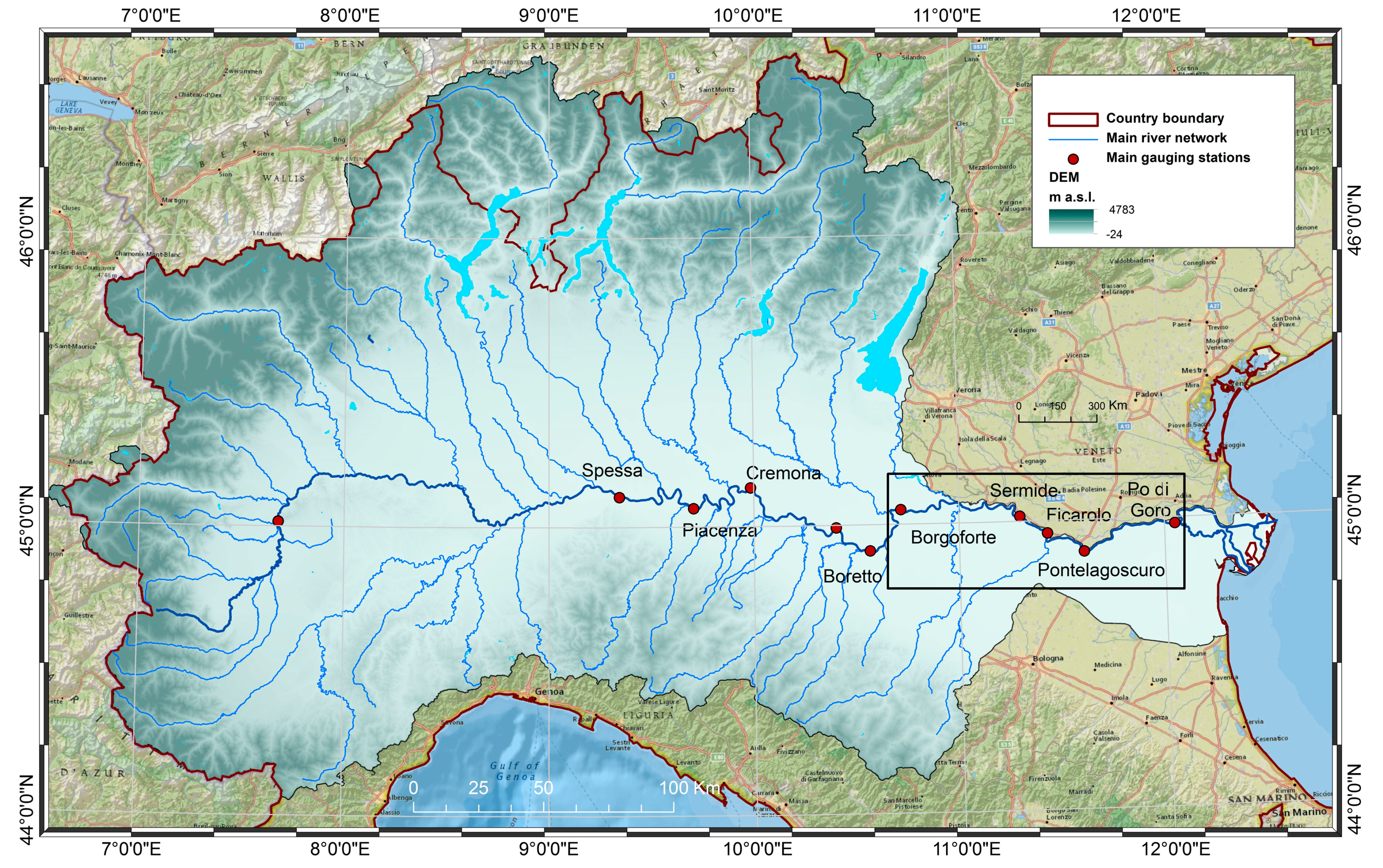
This study focuses on the Po River, the longest and widest Italian river, along which a number of gauged stations, to provide long series of observed water levels and discharge values (see Figure 1). The analysis is carried out for a river reach of 137 km from the gauged station of Borgoforte to Po di Goro, the beginning of the river delta, including also three other gauged stations, Sermide, Ficarolo, and Pontelagoscuro, which we used for comparison purpose (see the box in Figure 1). Along this portion the main river width ranges from 200 m up to nearly 500 m, while the lateral floodplains are delimited by a system of major embankments and may reach an extent of 5 km. In light of its geometrical characteristics and the amount of available hydrological observations, this river portion represents an ideal test case for the satellite mission so that it has been previously considered for the investigation of SWOT potential (see, e.g., [19,25,27]).
Different from previous studies we selected a study period of three years, from January 2008 to December 2010, during which the river experienced both major floods and drier periods. Figure 1 shows the overall Po River Basin, the study area (box) and the gauging stations where mean daily discharge values and water levels have been recorded for many decades.
As an example, Figure 2 reports the daily mean discharge values during the period in interest at the gauging stations of Borgoforte (upstream station) and Sermide as reproduced by the numerical model (see Section 2.3 for more details). As depicted in Figure 2, the Po River in this short period experienced two significant floods (May 2009 and 2010) and a series of minor peaks. This reference period enables the evaluation of all possible flowing conditions along the river.
Table 1 summarizes principal hydrological characteristics of the gauging stations with reference to the three-year period of interest (2008–2010) and the overall historical monitoring period.
2.2. SWOT Mission: Scientific Background and Satellite Coverage
The SWOT mission is led by the National Aeronautics and Space Administration (NASA) and the French space agency (Centre National d’Études Spatiales, CNES), in collaboration with the Canadian and UK space agencies (CSA and UKSA, respectively). The purpose of the mission is to contribute to the fundamental understanding of the Earth system by providing high spatial resolution and global measurements for ocean and inland water. Specifically, for terrestrial water bodies, it will provide a global inventory of lakes, reservoirs, and wetlands, whose surface area exceeds 62,500 m2 and rivers whose width exceeds 100 m (hopefully 50 m). Moreover, it will enable the estimation of river and global storage variation at sub-monthly, seasonal, and annual time scales by providing water extent, water surface elevation, and slope (see, e.g., [24,26] for more details).
The core payload includes a Ka-band radar interferometer (KaRIn, 35.75 GHz, or 8.6 mm wavelength) with a near-nadir incidence angle. Regarding the spatial coverage and the revisit time, the global measurement ranges between 78°S to 78°N, with a revisit time of about 21 days. Starting from radar observations based on pixels having the size of about 6 m in the azimuth direction, and ranging from 10 to 60 m in the direction perpendicular to the azimuth, SWOT products will be the result of averaging procedures aimed at achieving the mission requirements in terms of observation accuracy [24,25,27]. Satellite products will be available within two swaths of 50 km width and separated by a gap of 20 km (“nadir gap”), one on each side of the satellite. For additional technical details on the SWOT mission the reader can refer to [24,26,28], whilst more information concerning SWOT data products are reported in Section 3.1.
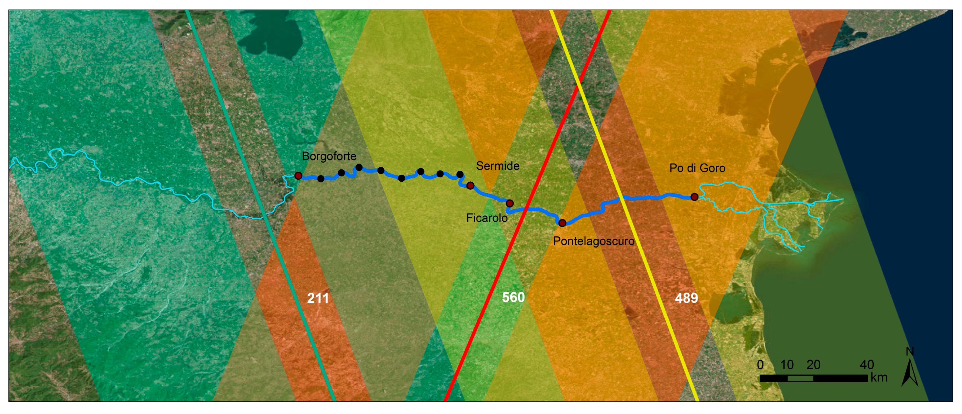
Looking at designed satellite orbits, the Po River reach under investigation is intercepted by three SWOT orbits: 560, 489, and 211. As an example, and referring to Figure 3, orbit 560 observes the study area with both swaths (left and right, or also 560 up and 560 down, respectively; orange surfaces in the figure), except for the 20 km of the nadir gap. Starting from the upstream gauged station of Borgoforte, the upstream swath (560) observes 68.3 km of the river reach. The same river portion is observed from orbit 211 (right swath, green area in Figure 3). The 560′s downstream swath includes the river from Pontelagoscuro up to the final section of the model. The upstream (left) swath of orbit 489 observes 79.3 km of the river, covering the nadir gap of the orbit 560. The downstream (right) swath of 489 observes the eastern part of the reach. However, in light of its small extent, this portion is considered insignificant for the analysis and, thus, neglected. As depicted in Figure 3, the river stretches of about 44.1 km, including the gauged section of Sermide, is monitored by the three orbits, and it would receive three observations within the period of 21 days (i.e., satellite revisit time).
Referring to the flow hydrograph at the gauging stations of Borgoforte and Sermide, Figure 2 shows the satellite coverage of this river portion during the three-year period of interest (vertical lines). Under the hypothesis that orbit 560 overpasses the Po River on 1 January 2008, orbit 211 would cross the river 10 January (nine days later), while the 20th of the same month (19 days later than orbit 560) the Po would be monitored along satellite track 489 (see Figure 2 and Figure 3). This observation sequence is repeated every 21 days, resulting in a total number of satellite overpasses equal to 157, of which 52, 53, and 52 refer to orbit 489, 560, and 211, respectively.
2.3. Hydrodynamic Simulation of the River
In order to mimic remote observations expected from SWOT, we implemented a quasi-two dimensional hydraulic model using UNET code, which solve the one-dimensional Saint Venant equations by means of a classic implicit four-point finite scheme [29]. The model refers to the software Hydrologic Engineering Centre–River Analysis System, HEC-RAS, developed by the United States Army Corps of Engineers. The numerical model is implemented according to a quasi-two dimensional structure that considers the one-dimensional flow in the main channel and schematizes the dike protected floodplains as storage areas connected to the main channel through lateral structures (see, e.g., [30]). In consideration of these structures, the dike-protected floodplains start to be flooded when the water level overtops the minor embankment system, and the water volume of the storage areas is simulated through depth/flood volume curves retrieved by the digital elevation model. The river geometry is described by 107 cross-sections extracted from a 2 m resolution LiDAR survey performed in 2005 and integrated with sonar bathymetry profiles performed by the Po River Basin Authority (AdB-Po). Previous analysis performed on the same area shows the suitability of the quasi-2D model for the simulation of the hydraulic behaviour of the river, enabling the reconstruction of realistic daily flow conditions (the reader is referred to [31,32] for additional details on the model calibration and validation). In this context, it is worth mentioning that the study aims to investigate the potential of SWOT sensors on the estimation of hydraulic variable and river discharges as synthetically generated by the model rather than reproducing the real behaviour of the river. Simulations obtained with the numerical model can be considered as a synthetic reality that represents the river behaviour, thus, we can use them to mimic SWOT observations (see Figure 2). Based on this approach, the comparison of SWOT-derived FDCs with those obtained with three years of simulated data is fair and it is not affected by possible biases introduced by the numerical simulation. Adopting this approach, the numerical model enables us to mimic the spatial coverage of the satellite and provides hydraulic variables that are not available from traditional gauging stations. As a result of the hydrodynamic simulations, daily hydraulic variables, such as the water surface level, water extent, wetted area, discharge, water depth, etc., are available at each river cross-section along the study area (Figure 3; dark blue) for the period of interest. For the numerical simulation, daily streamflow values are used at the gauging station of Borgoforte, whilst the downstream boundary condition is reproduced by imposing the normal flow condition at the beginning of the river delta (see Po di Goro in Figure 3).
3. Methodology
Referring to rivers, SWOT will provide information in terms of water surface width, , water surface elevation, , and slope, . Although the characteristics of SWOT products are still under definition, the results of recent investigations offer useful indications and sustain a cautious optimism regarding the achievement of mission requirements [16,25,27]. This work refers to these latest experiences for the estimation of river discharges along the study area.
3.1. River Reach Discretization
SWOT will provide spatially continuous information along the sensed swath. Radar “raw” measurements retrieved from the sensor will be spatially averaged in order to provide the final products and ensure the achievement of designed accuracy [25,26,28]. Thus, SWOT products, such as water surface elevation, water extent, and water slope, will be delivered with reference to different river stretches. Frasson et al. [25] investigated automated strategies for river discretization, comparing the effect on product accuracy of dividing the river into reaches of arbitrary lengths, with others identified with reference to hydraulic controls (e.g., tributaries, dams, etc.) or changes in river sinuosity. Although the analysis shows better performances on discharge estimation for the two latter approaches (i.e., hydraulic controls and sinuosity), errors on water heights and slope were comparable with those obtained dividing the river into stretches of arbitrary lengths (e.g., lengths varying from 2 km to 25 km). In general, the longer the arbitrary stretch length adopted, the lower the error, or bias, introduced into the SWOT products [25].
Based on these conclusions, and for the sake of simplicity, in this study we adopted constant stretches. However, in order to evaluate if the extent of the stretches has an effect on our application, the analysis is conducted for three different lengths, Δx equal to 5, 10, and 20 km. Table 2 indicates the number of stretches included within each swath. Each of these stretches is identified as a collection of consecutive river cross-sections within a given Δx distance among those considered. Based on these assumptions, simulated variables obtained from the hydraulic modelling (i.e., water elevation, slope, water extent; see Section 2.3) are averaged with reference to those river stretches. As an example, black dots in Figure 3 identify those river stretches identified along one of the satellite swaths (i.e., 560 upstream) adopting a discretization length of 10 km.
3.2. Simulation of SWOT Hydraulic Variables and River Discharge Estimation
Since investigative studies are needed before the planned launch of the satellite in 2021, and in line with previous studies that investigated SWOT potential [10,15,16,33], we reproduce the satellite observations by corrupting the simulated hydraulic variables (such as water level, water surface width, and slope) with errors consistent with the expected performance requirements [26]. In other words, for the scope of the analysis, water levels and other hydraulic variables obtained from the numerical simulations represent the synthetic reality that we refer to in order to simulate SWOT observations.
In this study, the estimation of the river discharge from SWOT observation follows the approach previously used by Frasson et al. [25] and Durand et al. [15], who applied the Manning equation for each day of passage and for each branch. We assumed that the water surface slope () can approximate the friction slope () and that the width of the river is significantly larger of its height, thus reducing the wet perimeter equal to (water extent). Under these assumptions, the Manning equation is:
where denotes the wetted area and (m−1/3s) is the Manning coefficient. Once the day of passage, j is identified, we discretized in i-branches of length ∆x the river portion observed in the satellite swath (see Section 3.1 and Figure 3). The average value of the hydraulic variables, such as wij and Aij, is calculated by averaging, in space, the values observed during the j-th day at all the cross-sections included in the i-branch.
The wet flow area at a given location in a specific day can be written as:
where represents the average value of the minimum wet areas recorded for the i-th branch during the entire period of study. indicates the flow area variation with respect to the minimum value and it is calculated as:
where is the average value of the minimum width recorded for the i-th branch.
The roughness coefficients, n, vary from 0.025 to 0.044 (m−1/3s) moving from downstream to upstream and are derived from previous investigations performed along the study area [32], in accordance with the literature [34]. Since , , cannot be inferred from SWOT we adopted a simplified approach in which those variables are extracted from the hydraulic model with reference to the minimum flow condition experienced in the period of interest.
The water surface slope, S, is evaluated by interpolating the water height values, y, considered for all river cross-sections of each branch, as follows:
where x represents the progressive abscissa along the river. The interpolation to obtain values required in Equation (1) is performed along each i-th river stretch considering every j-th sensing day.
Similarly to the simplifications adopted in previous studies [24,26], errors attributed to remote measurements are simulated by corrupting the values extracted by the hydraulic model with Gaussian random errors, with mean equal to 0 and standard deviation equal to the expected performance requirement specified for each variable. Specifically, = 0.1 m for the height (), = 1.7 × 10⁻⁵ for the slope () and = 0.15 times the water surface extent ([24]).
Based on these assumptions, given a specific orbit overpass, j, and a river discretization length, Δx, we first calculate the spatial mean of the hydraulic variables based on the data simulated at all river cross-sections within a i-th stretch (yij, wij, Aij). Finally, those values are corrupted with random errors and used to solve the Manning equation (Equation (1)) for the calculation of reach-averaged discharge, .
Equation (1) can finally be written as:
where the hat symbol identifies variables estimated from SWOT and, thus, the variable corrupted with random errors.
To consider the uncertainty on the error generation process we refer to a Monte Carlo technique obtaining 1000 values, , of simulated discharge for each branch and for each satellite passage.
The mean of the iterations can be depicted as the following:
where k is the k-th value of simulated discharge.
The benchmark discharge, called , is calculated referring to river flows provided by the hydraulic model, , and spatially averaged considering the adopted river stretches as follows:
where is the number of river cross-section within a given stretch of length Δx (5, 10, or 20 km).
3.3. Flow Duration Curve
Discharge estimated by means of Equation (5) can be used to construct the FDC of a given river stretch and provide information on the percentage of time that a discharge is equally, or exceeded, during a reference period. In particular, the FDC is obtained by sorting the discharge time series in descending order, assigning to them a duration calculated as a percentage, from 0 (higher value) to 100 (minimum value), of the observation period.
Both simulated and estimated discharge time series are represented in terms of FDC. In addition, within the scope to evaluate the representativeness of SWOT lifetime for the estimation of the river flow regime, FDCs based on SWOT-like observations are compared with those based on long observation periods, thus using discharge values recorded at the gauging stations reported in Table 1.
3.4. Performance Indices
We evaluate the performance of the applied approach for the estimation of the river discharge through the calculation of different performance indices: the coefficient of determination, R2, the root mean square error, RMSE, and the mean absolute error, MAE, which have been evaluated both in terms of absolute (m3/s) and relative (rRMSE and rMAE expressed as a percentage) values. Those performance indices have been evaluated referring to each sensed river stretch (RMSEij, MAEij, rRMSEij, rMAEij) for each satellite overpass:
where N represents the number of iterations within the Monte Carlo framework.
4. Results and Discussion
4.1. Discharge Estimation
The scatterplot in Figure 4 illustrates the comparison between the estimated and the simulated, discharge for each discretization Δx, considering all satellite overpasses in the study area during the three years. Referring to discharges estimated with Equation (5), Figure 5 shows the errors in terms of rRMSE and rMAE in relation to the streamflows for the left swath of orbit 560 (also named 560 upstream, 560 up; see Table 2), and orbit 211, which partially monitor the same river portion (see Figure 3). Table 3 summarizes all the errors, reporting the mean performance indices values for each orbit and discretization. For the sake of brevity, plots regarding other SWOT orbits are reported as Supplementary Materials (Figures S1–S4).
Generally, points lie above the bisector, even if, for high discharge values, a larger spread is observed. Larger errors are obtained in the case of Δx equal to 5 km (red points in Figure 4), especially during high flows. The adoption of Δx equal to 10 and 20 km (blue and green points, respectively) provides comparable results, except for high flows, where the longer the averaging length, the lower the expected error. Between these two options, Δx = 20 km is the one associated with better performances, especially in the range of low flows where the difference compared to Δx = 5, 10 km is more evident (see Figure 5). Adopting this discretization, the rRMSE and rMAE always remain lower than 20% for medium to high flows, with the only exception of the swath 560 downstream (see Figure 5 and Figures S2 and S4 in the Supplementary Materials). Determination coefficients (R2) reported in Figure 4 provide a measure of the performance of the applied methodology in estimating the flowrates, with values always higher than 0.9. Δx equal to 10 km ensures the larger R2 value, while a lower performance is obtained in the case of longer discretization (i.e., Δx equal to 20 km) because of the overestimation of low flows (green dots in Figure 4).
Looking at the panels in Figure 5 (and others in the Supplementary Materials) it is evident that large errors on the discharge estimation are expected in the case of adopting short averaging lengths: Δx equal to 5 km. This result is somewhat expected, since the information averaged along a short reach is more affected by local errors than along a longer reach. This appears evident for a small number of river reaches (the lower set of red points in Figure 4) where the limited averaging length adopted does not remove possible local errors introduced by the assumptions of Equation (5). This is confirmed by the values of Table 3, with the only exception of orbit 560 downstream, where the average error is comparable to the one found for Δx = 20 km. Worse results associated to swath 560 downstream are probably related to the hydraulic characteristics of the river near the delta, where the low river slope and its limited width in this portion significantly affect the discharge estimation, especially for low flow values.
Confirming the results of Frasson et al. [25], the larger the streamflow, the lower the expected relative error: in general, both rRMSE and rMAE decrease when discharge increases. Larger errors in the case of low flows are probably due to the effect of hydraulic simplifications adopted in Equation (5), which become more significant when only a small portion of the river section is flooded. This also explains the error peak that is generally observed (at all stations, and for all river discretizations) for discharges between 1000 and 1500 m3/s, when the river flowrates start flooding the lateral floodplains and the assumption of a rectangular river shape appears far from the real conveyance conditions.
4.2. Spatial and Temporal Monitoring of the Study Area
To provide an overview of the spatial and temporal monitoring expected from SWOT Figure 6 reports an example of the river monitoring estimated from one of the satellite overpasses (namely 560, overpasses no. 53) simulated during the three year of mission lifetime. Referring to ∆x = 10 km, red segments in Figure 6 indicate the mean discharge values obtained from the numerical model (i.e., , Equation (7)), while blue triangles report SWOT-based streamflows (; Equation (6)). The spatial distribution of the estimated values (triangles) depicts the coverage of the two satellite swaths (left and right), which are separated by a nadir gap (~20 km) where no data will be observed by the satellite (see also Figure 3).
In order to provide an overall view of the temporal sampling of the flow hydrograph, and corresponding errors, we compared the estimated and simulated discharges at the four gauged stations along the river (Borgoforte, Sermide, Ficarolo, and Pontelagoscuro; see also Figure 1 and Figure 3). The comparison is made referring to river flow values averaged along the river stretch, of length Δx, within which each gauging station falls.
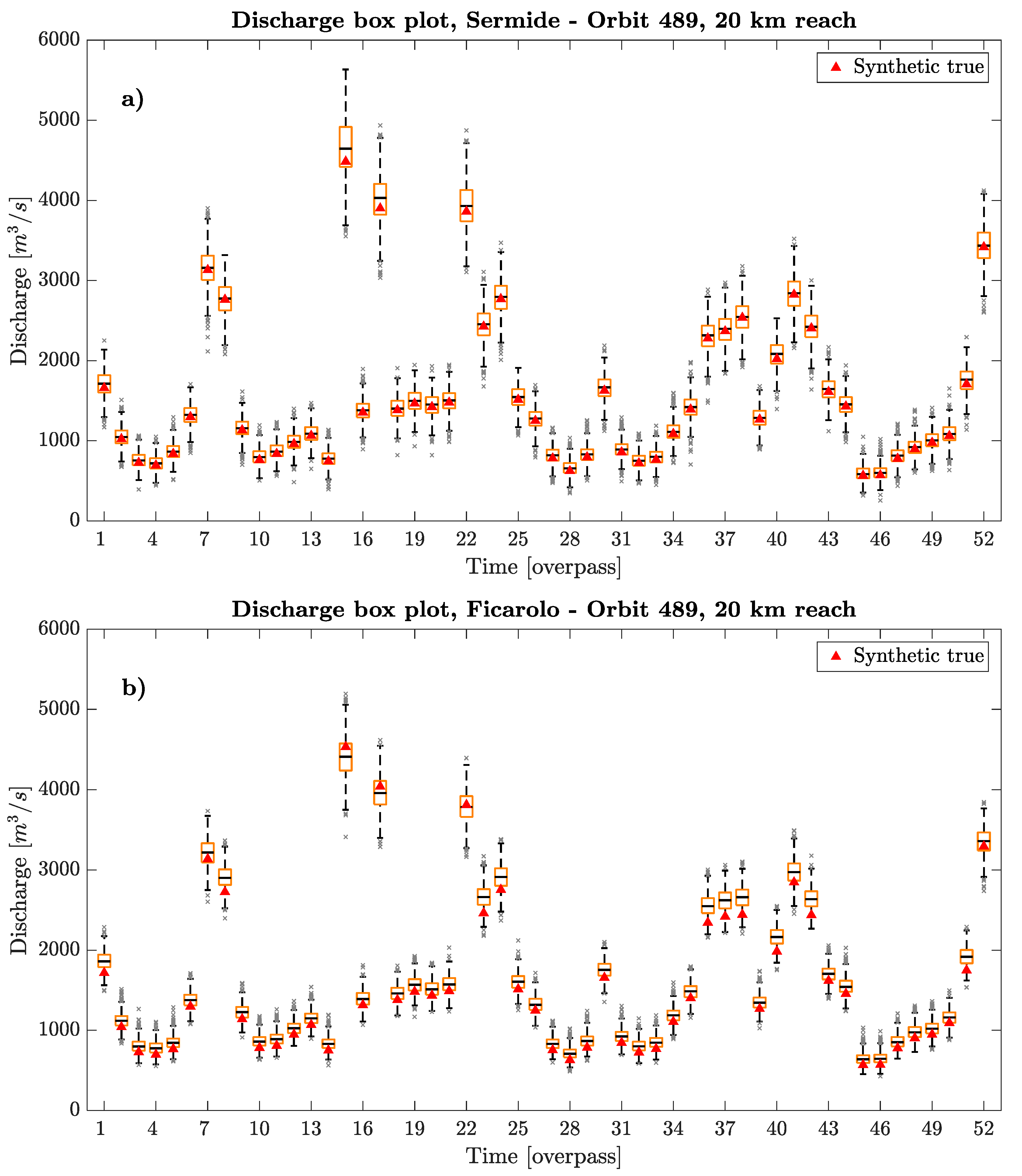
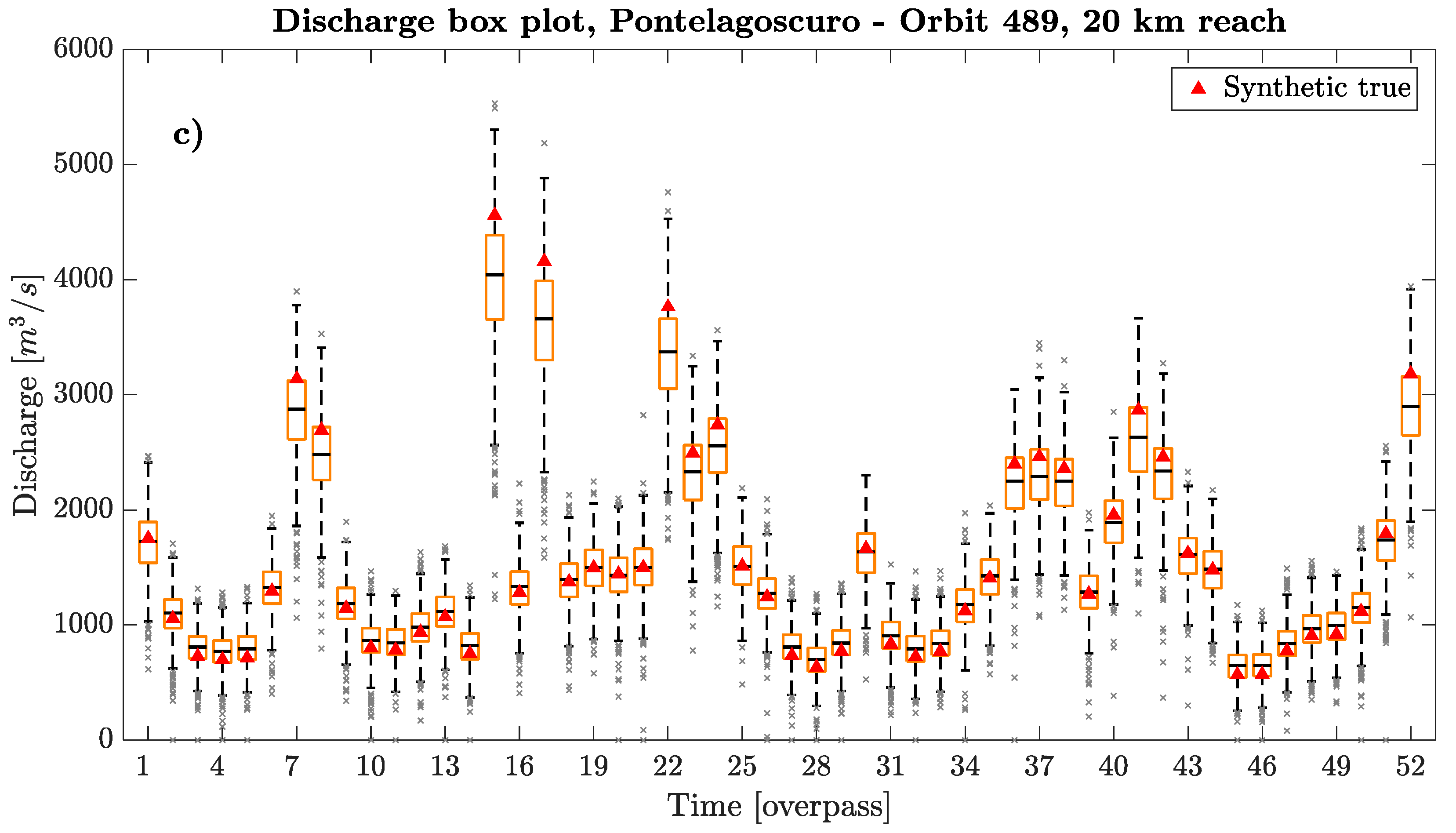
Figure 7 reports the boxplots of the N estimated discharges (; Equation (5)) along with the synthetic values (, Equation (7); red triangular) at the gauging station of Sermide, Ficarolo, and Pontelagoscuro. Similar plots regarding other gauging stations are reported in the Supplementary Materials (Figures S5–S8). Each boxplot gives an idea of the dispersion of the N (1000) discharge values simulated in that specific river stretch during a given SWOT overpass. It is worth highlighting that the total number of boxplots (i.e., x-axes) indicates the number of times the river stretch has been monitored by the satellite during the mission lifetime (see Section 2.2). For brevity, we report here only the discretization of 20 km, but similar results are available for 5 and 10 km in the Supplementary Materials.
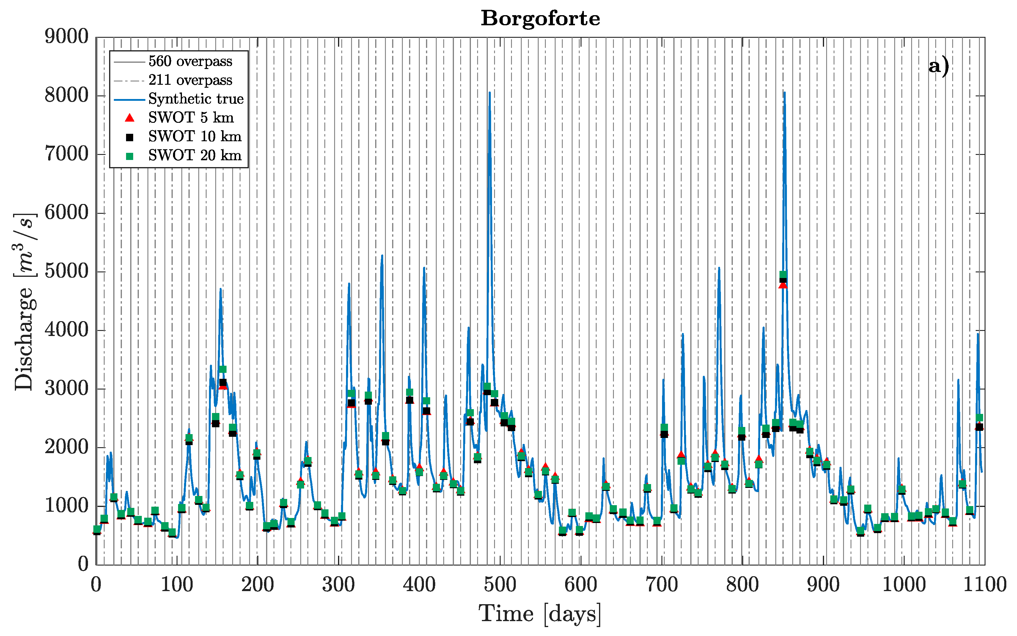
Figure 8 provides a final overview of the temporal sampling overlapping the daily flow hydrograph with discharge estimations considering different discretization lengths (Δx). In particular, referring to the mean discharge value obtained from Equation (6) (), plots of Figure 8 summarize the potential of SWOT in observing the variability of the streamflows during the mission lifetime overlapping the discharge estimation with flow hydrographs observed at the available gauging stations. Vertical lines indicate the satellite overpasses, while different symbols indicate the discharge estimations for the considered Δx.
As depicted in Figure 6, each SWOT overpass will guarantee the monitoring of a large river extent and, although the errors on reproducing the observed values (red segment), the satellite will enable the possibility to spatially monitor the river discharge and detect the rising and decreasing limbs. The availability of this data with a temporal resolution that varies from two to four visits within 21 days (see, e.g., [26]) will ensure a never before experienced knowledge of the river dynamic, with the opportunity to disclose new insights on flow propagation along the sensed rivers.
Results of Figure 7 further confirm that a longer averaging extent typically ensures lower estimation errors. The performances on discharge estimation appear quite variable along the river of interest, with the lower portion of the Po River characterized by larger biases (see, e.g., Pontelagoscuro). This is likely due to the geomorphologic characteristics of this river stretch, which denotes smaller river sections and lateral floodplains compared to the upstream part. Different river geometries may result on different performances on the estimation of the river flows according to the hypothesis introduced in this study (e.g., Equations (1)–(4)). In other terms, the impact of the simplifications introduced for inferring the river flow (e.g., the assumption of uniform flow, or concerning the estimation of the hydraulic radius; see Section 3.2) may not be the same along the overall river, introducing large errors in the same parts of the river. This also explains why, in some cases, a given gauging station experiences different errors in relation to the considered orbit (see, for example, the discharge estimation at Sermide when sensed by orbit 489 or 560). In fact, different swaths entail different river discretizations and, thus, the use of a different set of river cross-sections that fall within the river stretch of length Δx.
Results in Figure 7 highlight how performances are different for low and high flows: the range of variability of the errors is generally wider during floods than for low to medium flow conditions. Considering other gauging stations (see Supplementary Materials), the upstream section of Borgoforte underestimates high flows, whereas the approach at Ficarolo tends to overestimate low flows. This said, it is worth highlighting that observed discharges are generally included between the lower and upper extremes of the boxplot and, very often, they are in the range between the 25th and the 75th percentile.
Referring to the temporal sampling of Figure 8 it is evident how the sampling frequency varies in relation to the location. Ficarolo is monitored only by orbit 489 (52 observations in total during the mission lifetime), whereas the gauging station of Sermide is covered by three orbits (489, 560, and 211) and can rely on more observations during the mission (i.e., 157 in total).
This temporal sampling evidently influences the likelihood of the satellite to observe extreme events. Although peak flows in the Po River has a limited celerity and lasts for few days [35], it is evident from Figure 8 that high streamflows are generally missed by the satellite, even at Sermide, where the temporal sampling is more frequent than in other cases.
4.3. Estimation of Flow Duration Curve (FDC)
Figure 9 shows the results in terms of FDCs at the considered gauging stations, providing the percentage of occurrence of the estimated discharge during the monitoring period: duration values equal to 1% and 100% indicate the maximum and the minimum discharge value monitored during the observation period, respectively.
Black dashed lines indicate the FDCs based on daily discharge data simulated by the model (i.e., synthetic true) along the three-year period and are used as benchmarks for those based on discharge values sensed from the satellite. The comparison with these curves, even though built with synthetic discharge values, provides useful insights into the possible contribution of the future satellite mission in estimating FDCs. Curves of different colours refer to different river discretization lengths (Δx) and are constructed referring to discharge values estimated at the gauging stations at each satellite overpass. Specifically, these FDCs are obtained considering the median of the N discharge values, (see Equation (5)), estimated within the Monte Carlo framework. Adopting a discretization length of 20 km, the grey area in Figure 9 depicts the range of variability (90% of occurrence) of FDCs expected from SWOT in relation to the randomness of errors on the measurements of the water surface width, elevation, and slope (see Section 3). Similar areas can be drawn with reference to Δx = 5, 10 km, but are not shown in order to provide a clearer representation. In order to further investigate the potential of the mission for the characterization of the hydrological regime of the river Figure 9 also provides the comparison of FDCs constructed considering three-year (mission lifetime) data (black dashed lines) with those based on extensive (i.e., from 20 to 70 years) historical data (black solid lines; see also Table 1).
Figure 10 summarizes the variability of the errors between observed (black dashed line) and SWOT-based FDCs reporting the 90% confidence interval of the N errors on discharge values obtained for the different river discretizations (Equation (5)). Lines of different colours indicate the range of variability of the errors (90%) for the different discharge duration, referring to the considered river discretizations. Considering those ranges, Table 4 summarizes the results and reports the mean rMAE and rRMSE relative to the three-year observed FDC (the black dashed line in Figure 9).
Results from Figure 9 show a general overlapping among observed and SWOT-derived FDCs. Among the different discretizations, Δx = 20 km always ensures better performances, with the black dashed line always comprised within the 90% confidence interval (grey areas). This is also proven by the mean rMAE and rRMSE values obtained comparing observed and satellite-based FDCs and reported in Table 4: apart for the exception of Pontelagoscuro, error values associated with Δx equal to 20 km are the lowest. However, in general, mean errors are not significant and lower than 30%, 27%, and 16% for Δx equal to 5, 10, and 20 km, respectively.
Looking at Figure 9 and Figure 10, errors increase considering lower discharge. Results show a general overestimation of the streamflow values, which likely derives from the hypotheses introduced in the estimate of the river discharges. Simplifications on hydraulic radius and wet area estimation appear more robust for high flows while, for higher streamflows durations (i.e., low discharge on the river), the errors become more relevant.
The gauging station of Borgoforte is the one with higher performance, while higher biases are found at the remaining locations of interest. Referring to Sermide, the general discharge overestimation seen in Figure 9 decreases by considering longer river discretization (green curve; rRSME and rMAE equal to 6.6% and 5.7%, respectively). Similar behaviour can be seen at the gauging station of Ficarolo where the sensed FDCs have a similar shape as the observed one, apart from a limited overestimation that is not completely removed by also adopting Δx equal to 20 km.
In general, although the moderate number of observations provided by the satellite, which varies in relation to the location (see Section 3), the sensed FDCs seem able to reproduce the general shape of the ones built on daily data. As expected, the limited temporal sampling of the satellite reduces the likelihood of observing very large or low flows, resulting in large inaccuracies for the extreme values, both for high and low flows. This is evident also referring to Figure 8, which clarifies the sampling of the flow hydrograph at each gauging station. Referring to low flows, SWOT is expected to provide a large number of observations ensuring a significant coverage of streamflows associated with large durations. However, in this range of values, considering the limited river extent, water surface slope, and the possible effect of vegetation and infrastructures (e.g., embankments), the accuracy on streamflow estimation might be lower than for higher flows (e.g., [27]). On the contrary, high flows are rare and typically associated with a low duration in time, which reduce the likelihood of being monitored by the satellite. Figure 8 clearly highlights this aspect: the maximum flow values recorded during the study period would not have been sensed by the satellite. Thus, although high flows can be sensed with considerable accuracy, SWOT would probably not be suitable for the monitoring of low-frequency (i.e., one-day, two-day) streamflows.
While comparing short-period (i.e., three-year data; black dashed lines) with long-period (i.e., based on extensive historical data; black solid line) FDCs (Figure 9) it is worth noting that historical data are compared with discharge values derived from the numerical simulations, which may be affected by inaccuracies. Nonetheless, the representativeness and the performances ensured by the applied numerical model limit this risk (see also [31]). In general, the graphical comparison shows that an observation period of three years might provide a good understanding of the general hydrological behaviour of the catchment. As a matter of fact, the mean relative error calculated considering all possible discharge durations, long- and short-period FDCs (FDCs obtained using all historical datasets, or only a three-year period of data, respectively), is lower than 15%, precisely: 14.6% and 15% for Borgoforte and Sermide, respectively (panels (a) and (b) of Figure 9, respectively); 4.8% and 4.1% for the gauging stations of Ficarolo and Pontelagoscuro, respectively (panels (c) and (d) of Figure 9). Of course, flow over- or underestimation depend on the fact of observing a humid or dry period, while large inaccuracies are generally always expected for very high (low duration) or very low (high frequency) flows. Figure 9 clearly demonstrates these inaccuracies since both maximum and minimum flows historically observed at all the gauging stations are not properly sensed during the period considered in the study.
4.4. Potential and Limitations of the SWOT Mission for FDC Monitoring
Outcomes of this preliminary analysis show optimistic scenarios on the matters of SWOT-based FDCs. This first test case performed along the Po River demonstrates that the temporal sampling ensured by the mission should guarantee a river monitoring that enables a reliable estimation of the hydraulic regime of river. Considering a mission lifetime of three years, two or three overpasses within the satellite revisit time (21 days) appear sufficient to detect the range of variability of the river flows, even though extreme events (e.g., very high or low flows) might never be experienced during the mission lifetime or missed from the satellite. Starting from planned satellite orbits and satellite revisit periods, the scientific community is working on procedures that are aimed to synthetically improve the sampling of the hydrological observations, overcoming both temporal and spatial data sparsity. Amongst these approaches, data assimilation (DA) has been shown capable of providing valuable results for interpolating the flowrates along the river network observed by the satellite (see, e.g., [19,20]). Similar results have been obtained with statistical interpolation methods, such as kriging based approaches (see, e.g., [36,37]) or other spatiotemporal interpolation criteria (e.g., Inverse Streamflow Routing, [38]). These methods, even though they might require additional knowledge of the study area and heavier computational costs, they would allow a larger number of observations, thus enabling a more reliable representation of the hydrological regime of the rivers.
The comparison between observed and remotely-sensed FDCs highlights that the accuracy on the estimation of the river flows is probably the most relevant open issue to deal with for the estimation of FDCs, rather than the temporal sensing or the extent of the mission lifetime. In this context, under the assumption that the mission requirements will be achieved, the limited knowledge of the submerged river portions (i.e., river bathymetry, shape of the main channel) represents a relevant obstacle that strongly constrains the accuracy of the estimation. The lack of this information forces the adoption of simplifications and assumptions that do not always stand for all the river and flow conditions. This study overcomes these problems by using only a few fundamental assumptions, which include the adoption of the Manning equation to estimate the flowrate and the consideration of a rectangular shape with known bathymetry and friction coefficient. Regarding the first assumption, the Manning equation has been tested in previous works and, despite its simplicity, it was shown to provide results comparable with those from other, more complex, methodologies, especially in the case of large rivers, such as the one considered in our study [16,25]. On the other hand, the very limited availability, at the global scale, of high accuracy digital elevation models and river bathymetry data [39,40] would likely represent the most significant aspects confining the potential of the mission. The complexity of estimating river flowrates alongside the bathymetry and friction coefficient have led, up to now, to the development of simplified models based on Saint-Venant equations, as the one adopted in this case study. However, in the near future, DA may provide valuable techniques to overcome some of those constraints. For example, Oubanas et al. [19] have recently proposed a variant of the classical variational DA method (“4D-Var) that solves a nonlinear dynamic system where several variables, e.g., discharge, roughness, and bathymetry are estimated simultaneously. Mimicking SWOT observations over the Sacramento and the Po Rivers they were able to estimate the discharge in ungauged basins using only remote sensing information with promising results (with a relative root mean square error lower than 30%; [19]).
5. Conclusions
This study was aimed at investigating the potential role of the upcoming SWOT satellite mission for the estimation of flow duration curves (FDCs). These curves have a wide range of use in many hydraulic and hydrology-related activities, however, their generation relies on the availability of discharge records measured along the river. Since the progressive decline in stream gauge networks worldwide, the upcoming SWOT mission will definitely ensure a step forward for global freshwater monitoring, offering a proficient opportunity to extend our knowledge about the hydraulic regime of poorly-gauged rivers.
The analysis presented in this work refers to the 137 km portion of the Po River (Northern Italy) in light of the availability of traditionally-observed data and a quasi-2D hydrodynamic model of the river. Considering an artificial mission lifetime (three years, from January 2008 to December 2010) and the three planned satellite orbits (211, 486, and 560; see Figure 3) we mimicked the satellite observations by referring to the water surface width, elevation, and slope obtained from the numerical simulation and corrupted those with random errors according to the mission requirements [24]. Referring to those variables, discharge values have been estimated by adopting three different river stretch resolutions (Δx equal to 5, 10, and 20 km) following the approach of Frasson et al. [25] and Durand et al. [15].
The comparison between synthetic true and SWOT-based FDCs at the gauging stations demonstrates the satellite potential: discharge records expected from the satellite appear suitable to provide a reliable estimation of the flow regime at different locations. Among the tested discretizations, 20 km stretches provide better performances, with mean rMAE and rRMSE lower than 13.3% and 15.7% (see Table 4). Higher errors are expected at FDC tails, where very low or high flows have lower likelihood of being observed or might not occur during a limited mission lifetime period. Future applications will investigate the potential of spatiotemporal interpolation criteria (e.g., DA or statistical approach) that, within the limit of the mission lifetime (i.e., three years), are expected to ensure a denser spatial and temporal coverage of the river network.
Apart from encouraging results obtained with this analysis, it is worth noting here that the reliability and completeness of the acquired information on the hydrological regime will also depend on the hydrologic characteristics of the rivers (i.e., discharge variability, seasonality, etc.). Rivers with a limited variability of discharge will ensure a greater accuracy on the estimation of the FDCs, whereas for rivers characterized by fast flood waves and higher discharge variability, satellite monitoring might fail to capture all the hydraulic conditions. Future analysis will further investigate these aspects focusing on FDC sensitivity to the satellite overpass period, as well as on the importance of the river’s hydrologic regime.
Supplementary Materials
The following are available online at https://www.mdpi.com/2072-4292/10/7/1107/s1, Figures S1–S4: MAE, rMAE, RMSE and rRMSE for all satellite overpasses and swaths considering different discretization lengths (∆x = 5, 10, 20 km), respectively. Figures S5–S8: Boxplots of SWOT-based discharges compared with ones provided by the model (synthetic true; red triangle) at the gauging stations of Borgoforete, Sermide, Ficarolo and Pontelagoscuro, respectively, considering all sensing orbits.
Author Contributions
A.D. conceived and designed the experiments; L.G. performed the experiments; A.T. and G.S. assisted in analysing the data and contributed analysis tools; and all the authors wrote the paper.
Funding
G. Schumann’s time on this work was partially funded under a SWOT Algorithm Development Team (ADT) service contract from the NASA/Caltech Jet Propulsion Laboratory.
Acknowledgments
The authors are extremely grateful to the Interregional Agency for the Po River (AIPo) and the Po River Basin Authority (AdB-Po) for allowing access to their high-resolution DTM of the Po River and GIS layers used in the analysis. Data used for this work regarding the Po River are available upon request from the corresponding author (A. Domeneghetti: [email protected]). The authors are also grateful to the three anonymous reviewers for their meaningful and constructive comments.
Conflicts of Interest
The authors declare no conflict of interest.
References
- Pugliese, A.; Farmer, W.H.; Castellarin, A.; Archfield, S.A.; Vogel, R.M. Regional flow duration curves: Geostatistical techniques versus multivariate regression. Adv. Water Resour. 2016, 96, 11–22. [Google Scholar] [CrossRef]
- Vogel, R.M.; Fennessey, N.M. Flow duration curves II: A review of applications in water resources planning. JAWRA J. Am. Water Resour. Assoc. 1995, 31, 1029–1039. [Google Scholar] [CrossRef]
- Chow, V.T. Handbook of Applied Hydrology; McGraw-Hill Book Company: New York, NY, USA, 1964. [Google Scholar]
- Castellarin, A.; Galeati, G.; Brandimarte, L.; Montanari, A.; Brath, A. Regional flow-duration curves: Reliability for ungauged basins. Adv. Water Resour. 2004, 27, 953–965. [Google Scholar] [CrossRef]
- Ganora, D.; Claps, P.; Laio, F.; Viglione, A. An approach to estimate nonparametric flow duration curves in ungauged basins. Water Resour. Res. 2009, 45, 1–10. [Google Scholar] [CrossRef]
- Singh, K.P. Model Flow Duration and Streamflow Variability. Water Resour. Res. 1971, 7, 1031–1036. [Google Scholar] [CrossRef]
- Castellarin, A. Regional prediction of flow-duration curves using a three-dimensional kriging. J. Hydrol. 2014, 513, 179–191. [Google Scholar] [CrossRef]
- Tourian, M.J.; Sneeuw, N.; Bárdossy, A. A quantile function approach to discharge estimation from satellite altimetry (ENVISAT). Water Resour. Res. 2013, 49, 4174–4186. [Google Scholar] [CrossRef] [Green Version]
- Alsdorf, D.E.; Rodriguez, E.; Lettenmaier, D.P. Measuring surface water from space. Rev. Geophys. 2007, 45, 1–24. [Google Scholar] [CrossRef]
- Wilson, M.D.; Durand, M.; Jung, H.C.; Alsdorf, D. Swath-altimetry measurements of the main stem Amazon River: Measurement errors and hydraulic implications. Hydrol. Earth Syst. Sci. 2015, 19, 1943–1959. [Google Scholar] [CrossRef]
- Schumann, G.J.-P.; Domeneghetti, A. Exploiting the proliferation of current and future satellite observations of rivers. Hydrol. Process. 2016, 30, 2891–2896. [Google Scholar] [CrossRef]
- Bjerklie, D.M.; Dingman, S.L.; Bolster, C.H. Comparison of constitutive flow resistance equations based on the Manning and Chezy equations applied to natural rivers. Water Resour. Res. 2005, 41, 1–7. [Google Scholar] [CrossRef]
- Brakenridge, G.R.; Nghiem, S.V.; Andreson, E.; Chien, S. Space-Based Measurement of River Runoff. EOS Trans. Am. Geophys. Union 2005, 86, 185–192. [Google Scholar] [CrossRef]
- Gleason, C.J.; Smith, L.C. Toward global mapping of river discharge using satellite images and at-many-stations hydraulic geometry. Proc. Natl. Acad. Sci. USA 2014. [Google Scholar] [CrossRef] [PubMed]
- Durand, M.; Neal, J.; Rodríguez, E.; Andreadis, K.M.; Smith, L.C.; Yoon, Y. Estimating reach-averaged discharge for the River Severn from measurements of river water surface elevation and slope. J. Hydrol. 2014, 511, 92–104. [Google Scholar] [CrossRef]
- Durand, M.; Gleason, C.J.; Garambois, P.A.; Bjerklie, D.; Smith, L.C.; Roux, H.; Rodriguez, E.; Bates, P.D.; Pavelsky, T.M.; Monnier, J.; et al. An intercomparison of remote sensing river discharge estimation algorithms frommeasurements of river height, width, and slope. Water Resour. Res. 2016, 52, 4527–4549. [Google Scholar] [CrossRef]
- Birkinshaw, S.J.; Moore, P.; Kilsby, C.G.; O’Donnell, G.M.; Hardy, A.J.; Berry, P.A.M. Daily discharge estimation at ungauged river sites using remote sensing. Hydrol. Process. 2014, 28, 1043–1054. [Google Scholar] [CrossRef]
- Garambois, P.A.; Monnier, J. Inference of effective river properties from remotely sensed observations of water surface. Adv. Water Resour. 2015, 79, 103–120. [Google Scholar] [CrossRef]
- Oubanas, H.; Gejadze, I.; Malaterre, P.; Durand, M.; Wei, R.; Frasson, R.P.M.; Domeneghetti, A. Discharge Estimation in Ungauged Basins Through Variational Data Assimilation: The Potential of the SWOT Mission Water Resources Research. Water Resour. Res. 2018, 54, 2405–2423. [Google Scholar] [CrossRef]
- Andreadis, K.M.; Clark, E.A.; Lettenmaier, D.P.; Alsdorf, D.E. Prospects for river discharge and depth estimation through assimilation of swath-altimetry into a raster-based hydrodynamics model. Geophys. Res. Lett. 2007, 34, 1–5. [Google Scholar] [CrossRef]
- Tarpanelli, A.; Amarnath, G.; Brocca, L.; Massari, C.; Moramarco, T. Remote Sensing of Environment Discharge estimation and forecasting by MODIS and altimetry data in Niger-Benue River. Remote Sens. Environ. 2017, 195, 96–106. [Google Scholar] [CrossRef]
- Tourian, M.J.; Tarpanelli, A.; Elmi, O.; Qin, T.; Brocca, L.; Moramarco, T.; Sneeuw, N. Spatiotemporal densification of river water level time series bymultimission satellite altimetry. Water Resour. Res. 2016, 52, 1140–1159. [Google Scholar] [CrossRef]
- Tourian, M.J.; Schwatke, C.; Sneeuw, N. River discharge estimation at daily resolution from satellite altimetry over an entire river basin. J. Hydrol. 2017, 546, 230–247. [Google Scholar] [CrossRef]
- Rodriguez, E. Surface Water and Ocean Topography Mission (SWOT) Project Science Requirements Document; JPL D-61923; JPL: Pasadena, CA, USA, 2016. [Google Scholar]
- De Frasson, R.P.M.; Wei, R.; Durand, M.; Minear, J.T.; Domeneghetti, A.; Schumann, G.; Williams, B.A.; Rodriguez, E.; Picamilh, C.; Lion, C.; et al. Automated River Reach Definition Strategies: Applications for the Surface Water and Ocean TopographyMission. Water Resour. Res. 2017, 53, 8164–8186. [Google Scholar] [CrossRef]
- Biancamaria, S.; Lettenmaier, D.P.; Pavelsky, T.M. The SWOT Mission and Its Capabilities for Land Hydrology. Surv. Geophys. 2016, 37, 307–337. [Google Scholar] [CrossRef]
- Domeneghetti, A.; Schumann, G.J.; Frasson, R.P.M.; Wei, R.; Pavelsky, T.M.; Castellarin, A.; Brath, A.; Durand, M.T. Characterizing water surface elevation under different flow conditions for the upcoming SWOT mission. J. Hydrol. 2018, 561, 848–861. [Google Scholar] [CrossRef]
- Fjørtoft, R.; Gaudin, J.M.; Pourthié, N.; Lalaurie, J.C.; Mallet, A.; Nouvel, J.F.; Martinot-Lagarde, J.; Oriot, H.; Borderies, P.; Ruiz, C.; et al. KaRIn on SWOT: Characteristics of near-nadir Ka-band interferometric SAR imagery. IEEE Trans. Geosci. Remote Sens. 2014, 52, 2172–2185. [Google Scholar] [CrossRef]
- Preissmann, A. Propagation of translatory waves in channels and rivers. In Proceedings of the First Congress of French Association for Computation (AFCAL), Grenoble, France, 1961; pp. 433–442. [Google Scholar]
- Castellarin, A.; Di Baldassarre, G.; Brath, A. Floodplain management strategies for flood attenuation in the river Po. River Res. Appl. 2011, 27, 1037–1047. [Google Scholar] [CrossRef]
- Castellarin, A.; Domeneghetti, A.; Brath, A. Identifying robust large-scale flood risk mitigation strategies: A quasi-2D hydraulic model as a tool for the Po River. Phys. Chem. Earth Parts A B C 2011, 36, 299–308. [Google Scholar] [CrossRef]
- Domeneghetti, A.; Tarpanelli, A.; Brocca, L.; Barbetta, S.; Moramarco, T.; Castellarin, A.; Brath, A. The use of remote sensing-derived water surface data for hydraulic model calibration. Remote Sens. Environ. 2014, 149, 130–141. [Google Scholar] [CrossRef]
- Durand, M.; Andreadis, K.M.; Alsdorf, D.E.; Lettenmaier, D.P.; Moller, D.; Wilson, M. Estimation of bathymetric depth and slope from data assimilation of swath altimetry into a hydrodynamic model. Geophys. Res. Lett. 2008, 35. [Google Scholar] [CrossRef] [Green Version]
- Chow, V.T. Open-Channel Hydraulics; McGraw-Hill: New York, NY, USA, 1959. [Google Scholar]
- Montanari, A.; Ceola, S.; Baratti, E.; Domeneghetti, A.; Brath, A. Po River Basin. In Handbook of Applied Hydrology, 2nd ed.; Singh, V.P., Ed.; McGraw Hill: New York, NY, USA, 2017; pp. 1–4. [Google Scholar]
- Paiva, R.C.D.; Durand, M.; Hossain, F. Spatiotemporal interpolation of discharge across a river network by using synthetic SWOT satellite data. Water Resour. Res. 2015, 51, 430–449. [Google Scholar] [CrossRef] [Green Version]
- Yoon, Y.; Durand, M.; Merry, C.J.; Rodriguez, E. Improving temporal coverage of the SWOT mission using spatiotemporal kriging. IEEE J. Sel. Top. Appl. Earth Obs. Remote Sens. 2013, 6, 1719–1729. [Google Scholar] [CrossRef]
- Pan, M.; Wood, E.F. Inverse streamflow routing. Hydrol. Earth Syst. Sci. 2013, 17, 4577–4588. [Google Scholar] [CrossRef] [Green Version]
- Schumann, G.J.-P.; Bates, P.; Neal, J.; Andreadis, K. Fight floods on a global scale. Nature 2014, 507, 2014. [Google Scholar] [CrossRef] [PubMed]
- Domeneghetti, A. On the use of SRTM and altimetry data for flood modeling in data-sparse regions. Water Resour. Res. 2016, 52, 2901–2918. [Google Scholar] [CrossRef]
Figure 1.
Po River Basin, showing the main river network, gauging stations (red dots) and the river reach of interest (black box).
Figure 1.
Po River Basin, showing the main river network, gauging stations (red dots) and the river reach of interest (black box).

Figure 2.
Flow hydrograph at the gauging station of (a) Borgoforte and (b) Sermide (blue lines) in the period 2008–2010: vertical lines represent an example of the timing of the SWOT overpasses during a short period (see Section 2.2 for details).
Figure 2.
Flow hydrograph at the gauging station of (a) Borgoforte and (b) Sermide (blue lines) in the period 2008–2010: vertical lines represent an example of the timing of the SWOT overpasses during a short period (see Section 2.2 for details).


Figure 3.
SWOT satellite coverage of the study area: satellite orbits and swaths (different colours) over the river portion of interest (dark blue); red dots represent the gauging stations considered in the study; and black dots present an example of swath discretization (560 upstream) adopting Δx equal to 10 km (see Section 3.1).

Figure 4.
Scatter plot of synthetic (reproduced by the hydraulic model) and estimated (SWOT-based) discharges for each river stretch (Δx = 5, 10, 20 km) and for all satellite overpasses during the study period (2008–2010). The figure also reports the coefficient of determination (R2) between the discharge series for different Δx.

Figure 5.
Example of rRMSE and rMAE for two swaths observed by SWOT: orbit 560 (left swath) and orbit 211 (right swath; see also Figure 2).
Figure 5.
Example of rRMSE and rMAE for two swaths observed by SWOT: orbit 560 (left swath) and orbit 211 (right swath; see also Figure 2).

Figure 6.
Example of the spatial discharge monitoring expected from SWOT: synthetic true (red segments) and SWOT-based (blue triangle) discharges from orbit 560 (overpasses no. 53) considering Δx equal to 10 km.
Figure 6.
Example of the spatial discharge monitoring expected from SWOT: synthetic true (red segments) and SWOT-based (blue triangle) discharges from orbit 560 (overpasses no. 53) considering Δx equal to 10 km.

Figure 7.
Boxplots of SWOT-based discharges compared with ones provided by the model (synthetic true; red triangle) at the gauging stations of (a) Sermide, (b) Ficarolo, and (c) Pontelagoscuro, as sensed by orbit 489 and considering Δx equal to 20 km.
Figure 7.
Boxplots of SWOT-based discharges compared with ones provided by the model (synthetic true; red triangle) at the gauging stations of (a) Sermide, (b) Ficarolo, and (c) Pontelagoscuro, as sensed by orbit 489 and considering Δx equal to 20 km.


Figure 8.
Flow hydrograph sampling of the satellite at the four gauging stations considering all possible orbits and different river discretization lengths.
Figure 8.
Flow hydrograph sampling of the satellite at the four gauging stations considering all possible orbits and different river discretization lengths.


Figure 9.
FDCs at the gauging stations for the three-year period based on observed daily data (black dashed line) and estimated from SWOT-like observations, considering different river discretizations; grey area represents the 90% confidence interval of streamflow estimation with ∆x = 20 km; black solid lines show FDCs based on historical data recorded at the gauging stations.

Figure 10.
The 90% confidence intervals of the errors between FDCs obtained with synthetic true data (black dashed line in Figure 9) and those based on SWOT data at different duration and adopting different river discretizations.
Figure 10.
The 90% confidence intervals of the errors between FDCs obtained with synthetic true data (black dashed line in Figure 9) and those based on SWOT data at different duration and adopting different river discretizations.


Table 1.
Hydrological statistics available at the gauging stations of interest.
| Historical Data | Three-Year Period: 2008–2010 | |||||||
|---|---|---|---|---|---|---|---|---|
| Starting Year of Obs. (-) | Main Channel Width (m) | Min. Q (m3/s) | Mean Q (m3/s) | Max. Q (m3/s) | Min. Q (m3/s) | Mean Q (m3/s) | Max. Q (m3/s) | |
| Borgoforte | 1923 | 326 | 209 | 1312 | 12,047 | 466 | 1591 | 8060 |
| Sermide | 1994 | 485 | 123 | 1422 | 10,100 | 452 | 1661 | 7660 |
| Ficarolo | 1988 | 357 | 245 | 1557 | 11,200 | 560 | 1766 | 7580 |
| Pontelagoscuro | 1922 | 316 | 156 | 1509 | 10,300 | 534 | 1728 | 7090 |
Table 2.
Number of stretches identified for each swath based on the length of the discretization, Δx.
Table 2.
Number of stretches identified for each swath based on the length of the discretization, Δx.
| Δx [km] | 560 Up | 560 Down | 489 | 211 |
|---|---|---|---|---|
| 5 | 14 | 8 | 16 | 14 |
| 10 | 7 | 4 | 8 | 7 |
| 20 | 4 | 2 | 4 | 4 |
Table 3.
Mean values of RMSE and MAE (m3/s), rRMSE and rMAE (%) for each swath considering all overpasses over the Po River during the reference period.
Table 3.
Mean values of RMSE and MAE (m3/s), rRMSE and rMAE (%) for each swath considering all overpasses over the Po River during the reference period.
| MAE (m3/s) | RMSE (m3/s) | |||||
|---|---|---|---|---|---|---|
| Swath | 5 km | 10 km | 20 km | 5 km | 10 km | 20 km |
| 560 upstream | 146 | 144 | 118 | 177 | 173 | 175 |
| 560 downstream | 366 | 274 | 373 | 425 | 333 | 429 |
| 489 | 199 | 167 | 151 | 238 | 206 | 190 |
| 211 | 152 | 145 | 117 | 183 | 176 | 174 |
| rMAE (%) | rRMSE (%) | |||||
| 560 upstream | 10.3 | 10.1 | 8.4 | 12.5 | 12.3 | 12.7 |
| 560 downstream | 31.2 | 23.3 | 33.3 | 35.6 | 27.7 | 37.5 |
| 489 | 13.0 | 11.6 | 10.6 | 15.7 | 14.4 | 13.4 |
| 211 | 10.3 | 10.0 | 8.2 | 12.5 | 12.2 | 12.6 |
Table 4.
Mean rMAE (%) and rRMSE (%) obtained from the comparison of simulated and remotely-sensed FDCs at the gauging stations.
Table 4.
Mean rMAE (%) and rRMSE (%) obtained from the comparison of simulated and remotely-sensed FDCs at the gauging stations.
| rMAE (%) | rRMSE (%) | |||||
|---|---|---|---|---|---|---|
| Station | 5 km | 10 km | 20 km | 5 km | 10 km | 20 km |
| Borgoforte | 4.2 | 4.3 | 4.3 | 6.8 | 6.9 | 6.0 |
| Sermide | 28.3 | 14.6 | 5.7 | 29.2 | 15.2 | 6.6 |
| Ficarolo | 22.4 | 13.3 | 11.9 | 23.8 | 14.1 | 13.0 |
| Pontelagoscuro | 12.3 | 22.0 | 13.3 | 14.5 | 26.3 | 15.7 |
© 2018 by the authors. Licensee MDPI, Basel, Switzerland. This article is an open access article distributed under the terms and conditions of the Creative Commons Attribution (CC BY) license (http://creativecommons.org/licenses/by/4.0/).
Share and Cite
MDPI and ACS Style
Domeneghetti, A.; Tarpanelli, A.; Grimaldi, L.; Brath, A.; Schumann, G. Flow Duration Curve from Satellite: Potential of a Lifetime SWOT Mission. Remote Sens. 2018, 10, 1107. https://doi.org/10.3390/rs10071107
AMA Style
Domeneghetti A, Tarpanelli A, Grimaldi L, Brath A, Schumann G. Flow Duration Curve from Satellite: Potential of a Lifetime SWOT Mission. Remote Sensing. 2018; 10(7):1107. https://doi.org/10.3390/rs10071107
Chicago/Turabian StyleDomeneghetti, Alessio, Angelica Tarpanelli, Luca Grimaldi, Armando Brath, and Guy Schumann. 2018. "Flow Duration Curve from Satellite: Potential of a Lifetime SWOT Mission" Remote Sensing 10, no. 7: 1107. https://doi.org/10.3390/rs10071107
Note that from the first issue of 2016, this journal uses article numbers instead of page numbers. See further details here.