1. Introduction
Precipitation is an essential element of the global hydrological and energy cycles and its measurements are of great importance in a variety of research areas, such as climate studies, management of water resources, natural hazards and hydrology. In spite of its crucial role in many aspects of economic and social life on Earth, precipitation estimation still has many problems to overcome to meet the needs of hydrological and climate research and of operational applications.
Basically, precipitation is one of the most difficult atmospheric parameters to measure accurately as its estimate (from satellite and from the ground) is complicated by several factors: its large spatial and temporal variability; its phase (liquid and solid, mixed phase) and its composition in terms of different hydrometeor types, densities and sizes; problems in the conversion of radiometric measurements into quantitative precipitation estimates [
1,
2,
3,
4].
Rain gauge measurement are the only available direct measurement of precipitation, however they are affected by errors (e.g., effects of wind and evaporation) and suffer from their spatial distribution often too sparse over land to resolve rainfall intensity variability and virtually non-existent over the oceans [
5]. Ground-based weather radars, on the other hand, provide high-resolution indirect measurements of precipitation with uncertainties related to the conversion of reflectivity to rain intensity (calibration, range effects, beam-blocking, clutter, etc.) and their geographic coverage is inadequate for global precipitation monitoring.
These problems have highlighted the need to rely on satellite-based observations, which currently represent the most promising way for obtaining long-term global precipitation records. Although significant developments have been made, since the first measurements in the 1970s, quantitative precipitation estimation still poses several problems as the relation between surface precipitation rate and satellite-based observations is very complex. Remote sensing of precipitation from satellites is largely based on estimates made by observing some cloud top properties (e.g., cloud cover and cloud-top temperatures) in visible or infrared (IR) images, or by analysing the effects (absorption and scattering) of rain drops or large ice particles on microwave (MW) radiation. Since the early 1990s several studies have demonstrated that spaceborne passive microwave (PMW) observations have great potential for quantitative precipitation estimates because of the ability of MW radiation to penetrate the precipitating cloud (e.g., [
2,
6]). However, MW-based precipitation retrieval has to overcome some difficulties, such as: the inability to resolve the extreme variability of precipitation both temporally and spatially; the complex emission and scattering effects by hydrometeors on the upwelling radiation, associated to the extremely variable background surface conditions; the “ambiguity” (or “nonuniqueness”) in the relationships between the satellite observed spectral signatures and the surface precipitation [
7,
8,
9].
The launch of the Tropical Rainfall Measuring Mission (TRMM) (1997) has provided an important opportunity for the development of MW techniques, for the presence onboard of both a Ku-band precipitation radar (PR) and a PMW multi-frequency imaging radiometer (TMI). This has allowed the development of retrieval algorithms that have exploited the combined use of the information of the two sensors [
10,
11,
12]. Moreover, during its operational period the TRMM-PR radar has provided accurate estimates of instantaneous rain rate, as well as calibration for other precipitation-relevant sensors in sun-synchronous orbits [
13,
14,
15].
An important step forward towards the improvement of global precipitation monitoring has been achieved in 2014 with the advent of the Global Precipitation Measurement (GPM) mission, thanks to the availability of the NASA/JAXA GPM Core Observatory (GPM-CO) (equipped with the GPM conical-scanning Microwave Imager (GMI) and the Dual-frequency Precipitation Radar (DPR) (Ku and Ka band). The GPM mission contributes to the constellation of pre-existing and future radiometers onboard Low Earth Orbit (LEO) satellites and equipped with precipitation-sensing channels, ensuring 3-hourly global coverage between 65°S and 65°N [
16]. One of the GPM mission goals is to provide global precipitation products [
16,
17,
18] by harmonizing the different products obtained from the heterogeneous constellation of MW sensors. The Goddard Profiling Algorithm (GPROF), that is the NASA official PMW precipitation retrieval algorithm, is a well-known physically based (Bayesian) algorithm, aimed at this goal. Since its first release by Kummerow and Giglio [
19], it has continuously improved and evolved: Its current parametric approach allows its use in order to provide operational products for all PMW sensors available in TRMM and GPM era (1997 to present) [
7,
20]. In this same direction the EUMETSAT H SAF (Satellite Application Facility on Support to Operational Hydrology and Water Management) program [
21] has evolved to ensure optimal temporal and spatial monitoring of precipitation. This program, established in 2005, was designed to deliver satellite products (precipitation, soil moisture and snow cover parameters) mainly for operational hydrological applications and precipitation monitoring. The scientific collaboration established in 2014 between H SAF and GPM, endorsed by EUMETSAT and approved by the NASA PMM Research Program, has officially promoted a joint research activity towards development and refinement of retrieval techniques and validation strategies. In this context PMW instantaneous precipitation rate products exploiting all radiometers in the GPM constellation are being released within H SAF. These products are designed to be readily available and distributed in near-real time, also to be merged with GEO IR observations to provide high spatial and temporal resolution MW/IR precipitation products for operational applications.
The H SAF PMW precipitation products are based on two different precipitation retrieval approaches [
22]: the physically based Bayesian Cloud Dynamics and Radiation Database (CDRD) algorithm [
23,
24,
25], originally designed for conically scanning radiometers and the Passive microwave Neural network Precipitation Retrieval (PNPR) algorithm primarily developed for cross-track scanning radiometers, AMSU/MHS and ATMS [
26,
27]. In this work, a new algorithm based on the PNPR approach designed for the conically scanning GMI radiometer to provide global rainfall rate estimates for near-real time applications, is presented.
Artificial neural networks (NNs) represent a highly flexible tool alternative to regression and classification techniques, widely applied in an increasing field of environmental sciences for their capability to approximate complex nonlinear and imperfectly known functions to an arbitrary degree of accuracy (e.g., [
28,
29,
30]). The opportunities offered by their ability to learn and generalize and to be quite robust to noise, have encouraged their use in precipitation estimation from satellite and ground measurements, precipitation being, as mentioned, one of the most difficult of all atmospheric variables to measure. NN techniques have proven to be effective in this area of research and have been successfully used in many rainfall estimation and monitoring applications (e.g., [
31,
32,
33,
34]).
While previous versions of PNPR algorithms, developed for cross-track scanning radiometers AMSU/MHS (PNPR v1) and ATMS (PNPR v2) (H SAF precipitation products H02 and H18 respectively), were based on a training database obtained from cloud resolving model (CRM) simulations coupled to a radiative transfer equation (RTE) model, the new PNPR for GMI (hereafter referred to as PNPR v3) is based on an observational database. This database is built from global GMI-DPR observations during a period of 27 months between 2014 and 2016. The purpose was to develop a computationally efficient global precipitation retrieval algorithm able to handle the extremely large and rich observational database available from GPM-CO observations, meeting, at the same time, the H SAF requirement of delivering products useful to near-real time operations. It is worth noting that only liquid precipitation is considered in this work, while a separate module dedicated to snowfall retrieval from GMI measurements has been recently developed [
35] and will be soon incorporated in PNPR v3.
In this paper the design methodology of PNPR v3 algorithm for GMI is described in detail and the results of a verification study using the NASA DPR-GMI combined product [
36] are presented. Two case studies over Italy with a comparison of the PNPR v3 retrieval with co-located ground-based radar observations and with the GPROF (V5) instantaneous precipitation rate estimates, are also analysed.
Section 2 presents a brief description of the GMI radiometer characteristics.
Section 3 presents the relevant features of the observational database. In
Section 4 the design of the NN with the selection of the inputs is described and in
Section 5 the rain-no rain classification methodology is presented. In
Section 6 and
Section 7 the results of the verification study and of the two case studies are presented. Finally,
Section 8 provides the concluding remarks.
2. The GMI Instrument
The GMI aboard the GPM-CO is a multichannel, conical-scanning, total power MW radiometer equipped with 10 dual-polarization (V and H) window channels at 5 frequencies (10.65, 18.70, 36.5, 89.0 and 166.0 GHz) and three single-polarization (V) channels, one at 23.8 GHz and two in the water vapour absorption band at 183.31 GHz (V polarization).
All these frequencies are actually considered as the most appropriate for detecting the wide spectrum (heavy, moderate and light) of precipitation intensities [
16]. The four high frequency, millimetre-wave channels at 166 GHz and 183.31 GHz, can be exploited for light precipitation and snowfall retrieval at higher latitudes (e.g., [
37]). Having a low (407 km) orbital altitude and a 1.22 m diameter antenna, GMI can provide, on a 904 km wide swath, a better spatial resolution than most of the previous radiometers (up to roughly 4 km × 7 km at the high frequency channels and around 11 km × 18 km at 19 GHz). Moreover, compared to other radiometers, GMI has significant improvements in the calibration system [
38]. Because of these features, GMI represents a significant advancement in satellite PMW imagery.
The central portion of the GMI swath overlaps the Ku-band and Ka-band DPR swaths, 245 km and 125 km wide, respectively. The dual-frequency radar observations are beam-matched over the Ka-band swath, with a horizontal resolution of approximately 5 km and a vertical resolution of 250 m in standard observing mode. The measurements within the overlapped swaths of DPR and GMI are used to provide combined DPR-GMI products, besides DPR (dual-frequency and single frequency) and GMI (GPROF) products. These products serve as a precipitation/radiometric standard for the other GPM constellation members and are used to build a priori databases to support MW precipitation retrieval algorithms [
16,
17,
23,
39,
40].
3. The Observational Database
The approach based on NNs requires a “training phase”, that uses a large sample of data representative of the input and output variables of the retrieval process (in this case the TBs with ancillary parameters and the surface precipitation rate, respectively). The performance of the NN is largely dependent on the completeness and representativeness of the database and on its consistency with the actual observations. In this research, an observational database was used to train the NN. It is worth noting that a database derived from observations has various advantages over one provided by simulations of a CRM coupled to a RTE model. There are, in fact, some limitations associated with the use of CRMs, such as uncertainties in surface property characterization (e.g., surface emissivity), single scattering properties of ice or mixed phase hydrometeors, cloud microphysics parameterizations (particle size distributions, bulk densities, conversion processes), vertical and horizontal distribution of solid and liquid hydrometeors [
7,
8,
11,
23].
On the other hand, the use of observational databases is subject to other limitations such as calibration and stability, sensitivity of the instruments and accuracy of the precipitation products used as reference [
41,
42,
43,
44].
Table 1 presents the main characteristics of the observational database used in this research. The period analysed consisted of 27 months between 2014 and 2016, with about 1120 million observations (precipitating and non-precipitating). The GPM 2B-CMB product (version 04D), which combines DPR and GMI measurements, is used as reference [
36,
39]. In particular, the precipitation estimates used in the observational database are provided on the Ku-band radar swath and obtained from DPR Ku-band reflectivity and GMI brightness temperatures (1C-R product). Since only liquid precipitation is considered in this study, only pixels where 2B-CMB liquid fraction is larger than 0.8 are selected. The observational database is made of co-located vectors of GMI brightness temperatures (TBs) and 2B-CMB surface rainfall rate matching the GMI high frequency channel nominal resolution (4.4 × 7.2 km), with over 170 million precipitating and over 945 million non-precipitating elements.
It is important to add that, during the network design, the complete available database is normally divided into three parts: the ground truth (training) database to be used for the actual training (i.e., for estimating the parameters of the model), the validation database to be used for the verification of the performance of the trained NN and the test database, used to check the validity and usefulness of different NN models during the selection of the optimal NN (O-NN) (see
Section 4.2). The use of an independent test sample is generally quite effective in overcoming the overfitting tendency of NN models and for obtaining an unbiased estimate of the NN performance. These three databases are used, in different ways, in the NN design phase. In our study, we have reserved an additional (fourth) part of the database to be used in a verification study once the NN design has been defined.
It should be noted that all the selected databases need to be representative of all the precipitation events within the original complete database. The choice of the size and of the specific members of each database is thus crucial in obtaining an effective evaluation of the final NN performance. Bearing in mind that there are no general guidelines on how to split the complete database into smaller (four, in our case) parts, in our research the sizes of the four obtained databases were defined considering on one side the need to have sufficiently large and representative samples and on the other side the need to reduce the computation time. Considering that in the period chosen for the analysis (27 months), the coincident GMI-DPR pixels are about 170 million globally, in the design phase the sizes of the databases have been set at about 60, 30 and 30 million data for the training, validation and test databases, respectively. The size of the fourth database, reserved for a verification study on the final NN (PNPR v3) performance (
Section 6), has been set at about 50 million data. In order to ensure a homogeneous seasonal and spatial distribution of the GMI/ 2B-CMB pixels among the four datasets, an orbit by orbit selection with different steps depending on the relative size of the various databases was carried out. Moreover, a statistical analysis was made by dividing each dataset into four bins of precipitation rate (0.0001–1, 1–10, 10–30, >30 mm h
−1) and verifying that the percentage of occurrences in each bin was comparable for all the datasets.
4. PNPR v3
The new PNPR algorithm for GMI (PNPR v3) has been developed following the approach used for PNPR v1 and v2, (for AMSU/MHS and ATMS) in the NN design but with some important innovations (besides the use of the observational database): a new selection procedure of channels to be used as input to the NN, to fully exploit GMI capabilities for global precipitation retrieval (as opposed to the sounding capabilities of AMSU/MHS and ATMS [
45]); a reduction of the number of inputs, based on a new principal component analysis (PCA) approach; a new precipitation detection (screening) procedure based on a NN approach. Finally, unlike the previous PNPR algorithms designed for the Meteosat Second Generation (MSG) full disk area (60°S–75°N, 60°W–60°E), PNPR v3 provides precipitation retrieval over the whole globe (between 65°S–65°N).
However, some results of the previous PNPR approaches are retained in the new algorithm. The goal of using a single NN for different types of background surfaces has been preserved in the new version. Usually, the number of NNs used in the precipitation retrieval algorithms is defined so as to optimize the algorithm performance under different operating conditions. For example, distinct NN algorithms are proposed to deal separately with stratiform and convective precipitation (e.g., [
46]), or with different surface types (i.e., land or sea [
31]). However, the use of different networks can often lead to discontinuity of the estimates in correspondence with transitions between different conditions. The approach of a single NN-based algorithm requires a greater effort in the NN design phase and in the input selection but prevents discontinuities or inconsistencies in the retrieved precipitation patterns.
Another heritage of the previous PNPR algorithms is the use of the TB differences in the water vapour absorption band channels at 183.31 GHz as input to the NN. Opaque channels around 183 GHz were originally designed to retrieve water vapour profiles due to their different sensitivity to specific layers of the atmosphere (e.g., [
29,
47]). However, these channels have shown great potential for precipitating cloud characterization and for precipitation retrieval [
48,
49,
50,
51,
52].
4.1. The Neural Network
A detailed description of the neural network design process used in this work can be found in [
26,
27]. Here only a short summary is given, for the sake of clarity. A NN consists of a number of neurons (also called perceptrons) that exchange information with each other. The NN scheme, shown in Figure 2 in Sanò et al. [
26], is characterized by three blocks: (1) the input layer, that receives the input signals, (2) the hidden layer(s) and (3) the output layer, which provides the network response. Each layer holds a number of neurons determined, along with the number of hidden layers, during the design of the network. Each node has its own transfer function and receives, as input, a weighted sum of the outputs of the previous layer. The output of the transfer function corresponds to the output of each node.
The estimation of the weights of each neuron-neuron connection is performed in the NN training phase, during which a training database, providing the network with the inputs (e.g., TBs) and the expected output (e.g., 2B-CMB rainfall rate) is used and the value of each weight is modified to reduce the error between the network and the expected outputs. The training continues in order to minimize the error. At the end of the training, the final values of the weights connecting the neurons of the different layers, store the knowledge of the NN [
53]. The design of the network architecture is normally quite complex. Model selection in neural networks aims at finding as few hidden units and neuron-neuron connections, as necessary for a good approximation of the true function. Unfortunately, this is not a simple problem.
4.2. Input Selection and Design of Optimal Neural Network
An important step in the PNPR v3 development was the identification of the optimal set of inputs to the NN, and, the definition of one optimal NN (O-NN) able to provide global rainfall estimates (for all surface types). To this purpose, different typologies of TB-derived variables have been considered and several test networks were designed. In addition to the use of measured TBs in the different GMI channels, also their differences and their linear combinations to maximize the correlation with rain rate (following the CCA approach) [
23,
27], have been examined. Other TBs derived variables (e.g., Scattering Index (SI) [
54,
55], Polarization Corrected Temperature (PCT) [
32,
46,
56,
57] and TB-space transformation based on Principal Component Analysis (PCA) [
12,
31] were also analysed. For each set of inputs, the optimal NN (O-NN) was designed (in terms of number of hidden layer and perceptrons) following the cross validation procedure [
58,
59]. For a detailed description of the procedure see Sanò et al. [
26,
27].
In the cross validation strategy, the comparison between two models (two different NN for a given set of inputs in this case) is based on the mean square prediction errors (
MSPE) which is obtained applying the two models to different databases. For this purpose, a test database (see
Section 3) is used, divided into M subsets containing n observations each. The model is repeatedly applied to different datasets made of
n(
M − 1) observations, leaving out a different subset each time. The average
MSPE defines the cross-validation error,
CV:
In this procedure, the first step consists in determining the number of hidden layers of the NN for a given set of inputs. Starting from a simple architecture, two NNs are compared, one of which contains an additional hidden layer. For both NNs the CV is evaluated and, if the more complex unit shows a smaller CV error, the additional hidden layer is accepted. The procedure stops when no further hidden layer is able to reduce the CV error. At this point, with a similar procedure, the optimal number of perceptrons in each layer (for the same set of inputs) are found. Considering that there is a trade-off between these steps (the number of layers and the number of perceptrons in each layer are interdependent), the design procedure requires alternately tuning the number of layers, the number of perceptrons for each set of inputs. In order to obtain the O-NN about 100 NNs for each set of inputs were tested. Then the procedure was repeated modifying progressively the number or type of inputs and comparing the CV errors for the different O-NNs. The optimal set of inputs, associated to the O-NN with minimum CV error, was selected.
A preliminary analysis showed that the use of Principal Components (PCs) lead to low CV error compared to other tested input variables. Moreover, by estimating the variance of the signal associated with each component, it is possible to recognize the signal related to precipitation with respect to that of the background surface. Furthermore, the PCs selection procedure allows to reduce the size of the training database, simplifying the NN learning process.
The PCA approach was applied to all the GMI channels and to subsets of channels with similar characteristics, that is, water vapour absorption channels and low or high frequency window channels in double polarization. For each subset and for each surface type (vegetated land, arid land, ocean, coast), the PCs with correlation coefficient greater or equal to 0.7 were selected. Then the
CV approach was used to further reduce the number of PCs and to define four O-NNs (one for each surface type). Following Sanò et al. [
27], additional inputs were also considered in this phase: the TB difference in the 183.31 GHz channels (TB183 ± 3–TB183 ± 7 GHz), the surface height (altitude), the total precipitable water (TPW) derived from ECMWF Era Interim forecast (0.125° × 0.125° resolution). Two subsets, respectively composed of channels 10.6 GHz H/V, 18.7 GHz H/V (subset #1, 4 channels) and channels 36.5 GHz H/V, 89.0 GHz H/V, 166.0 H/V GHz (subset #2, 6 channels), produced the best results.
Table 2 lists the PCs selected for each surface type from subset #1 and subset #2. The different PCs are labelled as PCx.y where x is the subset index and y is the order of the PC in that subset (i.e., PC1.3 is the third order PC corresponding to subset #1).
The seven selected inputs are: the PCs listed in
Table 2 (three different PCs for each surface), the 183 GHz TB difference, the three ancillary variables (surface height, TPW and the surface type flag). The last step consisted in the design and development of one final O-NN able to provide global surface rainfall rate estimates over all the surfaces. As mentioned in
Section 4.1 the NN architecture is composed by three blocks: (1) the input layer, that receives the selected inputs, (2) the hidden layer(s), that contributes to the processing phase and (3) the output layer, that provides the surface rain rate estimate. The resulting NN architecture consists of one input layer with number of perceptrons equal to the number of inputs (seven) and two hidden layers with 23 and 10 perceptrons in the first and in the second layer, respectively. The tan-sigmoid transfer function is used for the input and the hidden layers, while a linear transfer function is used for the output node [
26,
27].
Table 3 shows the performance of the final O-NN compared with those of the O-NNs trained for different surfaces. The correlation coefficient computed on the test database (RCV) in the
CV procedure and the
CV, are indicated. From the table, it turns out that the final O-NN has performance that is on average better than the other NNs optimized for each surface.
It is worth adding that the resulting O-NN is extremely fast, allowing a processing time of about 2 min to retrieve the surface precipitation over a complete orbit using a computer equipped with an Intel-I7 processor and 16 Gb of ram.
5. The Rain/No-Rain Classification
In general, the identification of rain areas, or Rain/No-rain Classification (RNC) of pixels, represents a preliminary step to the MW precipitation retrieval and is considered crucial to obtain good performances of a PMW retrieval algorithm [
54,
60,
61,
62,
63].
In our study, the RNC has been based on the NN approach, designed following the
CV methodology already illustrated in
Section 4 and using the same observational database (
Section 3). However, some changes were made to the database in order to make it suitable for the discrimination between rain and no-rain areas. First, to the database used for the rainfall rate retrieval NN, consisting only of precipitating pixels, an equal number of non-precipitating pixels was added (about 350 million of elements). Secondly, the precipitation values were grouped into three categories labelled with three RNC flag values: 0 in the absence of precipitation (precipitation rate < 0.1 mm h
−1), 1 for precipitation rate between 0.1 mm h
−1 and 1 mm h
−1 and 2 for precipitation rate > 1 mm h
−1.
The RNC algorithm is based on two different NNs used jointly, each based on different input parameters. The use of two separate networks, was more convenient than the use of multiple parameters in a single more complex network, due to the extremely large size of the training database. This approach allowed us to fully exploit the potential offered by the 13 GMI channels. The first NN input selection was based on the PCA, as for the precipitation retrieval, with the addition of two TB-based indexes widely used for the RNC: the SI [
54,
55,
64] and PCT [
56,
65]. For the first resulting NN (SNN1), the inputs selected are: PCs listed in
Table 2, the 183 GHz TB difference, the SI and PCT (at 89 GHz), the surface type (vegetated and arid land, sea, coast) and the 2-m temperature (T2m), provided by the ECMWF forecast (0.125° × 0.125° resolution).
A second NN (SNN2), supporting the previous one (SNN1), was based on the use of polarization signal as input (TB differences between channels with same frequency and different polarization V and H) that can be very useful not only for the RNC itself but also for the surface characterization [
54,
66]. The inputs of SNN2 are: the surface type (vegetated and arid land, sea, coast), the ECMWF T2m and the polarization signal (TBv-TBh) of the 5 window channels at 10.65, 18.70, 36.5, 89.0 and 166.0 GHz.
According to the categorization of the training database (associated to three RNC flag values), the two networks return the outputs in terms of the same flag values (0, 1 and 2). A rain/no-rain classification index (RNCI) was therefore built by combining the outputs from the two NNs as shown in
Table 4. The value of RNCI is 0 when none of the two NNs detects precipitation (output flags equal to 0 for both SSN1 and SSN2). The value is 1 when only one NN detects precipitation (output flags 0 and 1–2 or 1–2 and 0, for SSN1 and SSN2 respectively). The value is 2 when both NNs indicate the presence of very light precipitation (output flags 1 for both SSN1 and SSN2). When the two NNs find precipitation but in different categories (output flags 1 and 2 or 2 and 1), RNCI is equal to 3. Finally, RNCI equals 4 when both NNs indicate precipitation rate greater than 1 mm h
−1 (output flags equal to 2 for both SSN1 and SSN2). With this criterion, in addition to exploiting the information of both networks, the RNC returns a parameter (RNCI) that can be used as a preliminary identification of areas with different rainfall intensity.
Some tests have been done and dichotomous statistical indices have been calculated in order to evaluate the performance of the screening. For this purpose, the new verification database (100 million data not included in the training/validation/test databases) was used and the 2B-CMB rainfall rate (grouped according to the RNC categories) was used as truth. Four cases corresponding to the four RNCI values were analysed and the POD (probability of detection; range 0 to 1, perfect score 1), FAR (false alarm rate; range 0 to 1, perfect score 0), CSI (critical success index; range 0 to 1, perfect score 1) and HSS (Heidke skill score; range −∞ to 1, perfect score 1) were calculated.
Table 5 shows the results obtained. As expected, the POD decreases and FAR decreases as the RNCI increases. CSI and HSS have a maximum value at RNCI equal to 2. The low values of CSI (and HSS) for RNCI ≥ 1, in spite of the POD = 0.96, is due to the high FAR found in this case (FAR = 0.65). Therefore, the best scores are obtained for RNCI ≥ 2 (i.e., when both SSN1 and SSN2 indicate a minimum of 0.1 mm h
−1 rainfall rate) and this threshold has been selected as the optimal rain-no rain flag indication for PNPR v3.
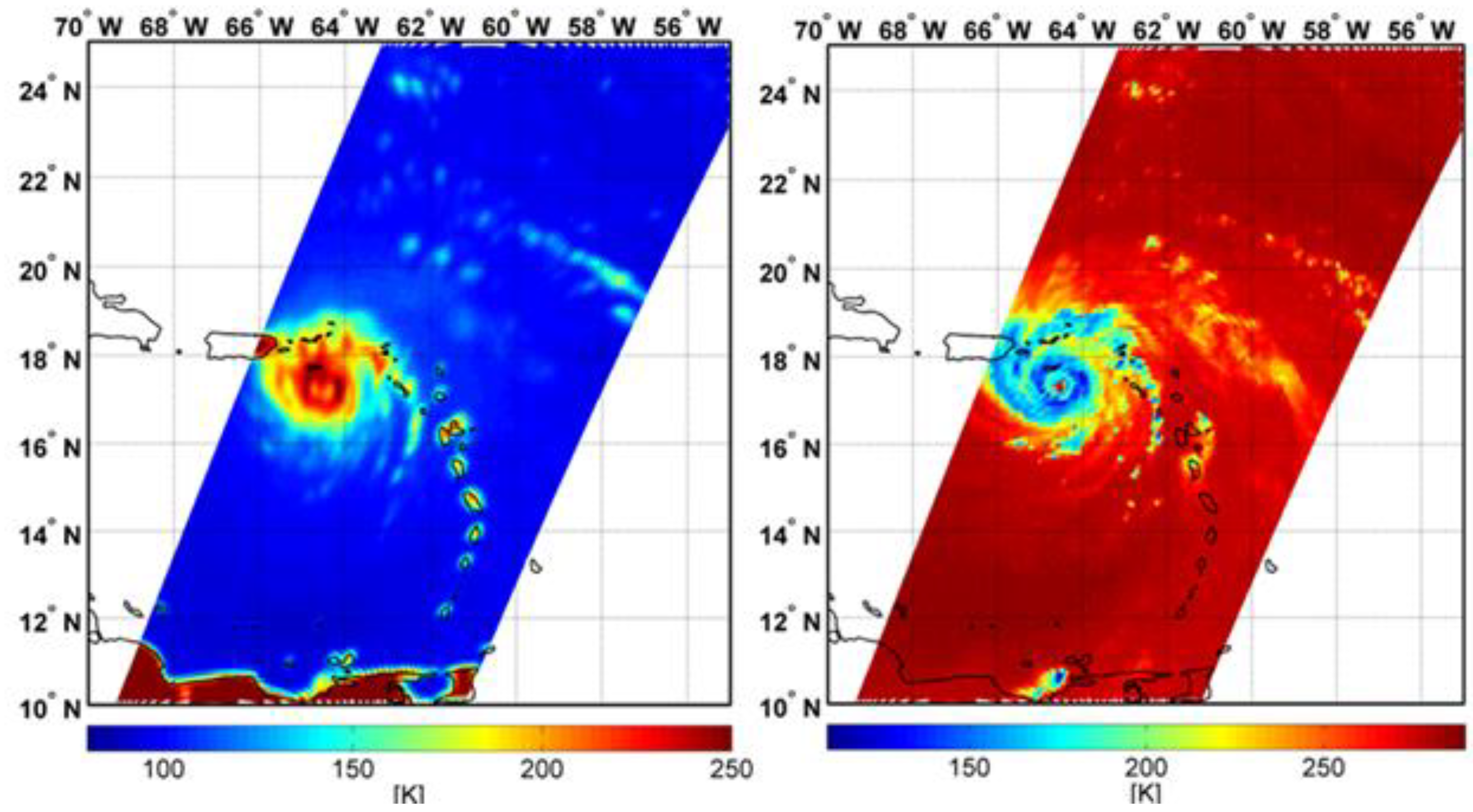
In order to illustrate an example of the effect of the different RNCI flags on the rain/no-rain pattern, the results of the screening scheme applied to one GMI overpass of Hurricane Maria near Puerto Rico on 20 September 2017 at 02:03 UTC are shown. Maria, a category 5 hurricane, was moving toward the west-northwest, over the extreme north-eastern Caribbean Sea. On 20 September, the centre of the hurricane was located southeast of Puerto Rico.
Figure 1 shows the measured TBs in the GMI channels at 10.7 GHz (H-pol) and 166.0 GHz (V-pol). The image clearly shows the structure and the eye of the hurricane, with the eye well defined at 166 GHz thanks to its high spatial resolution (around 5 km). Around the eye, regions of higher TBs at 10.7 GHz correspond to regions with lower TB at 166.0 GHz, likely representing convective precipitation embedded in the eyewall.
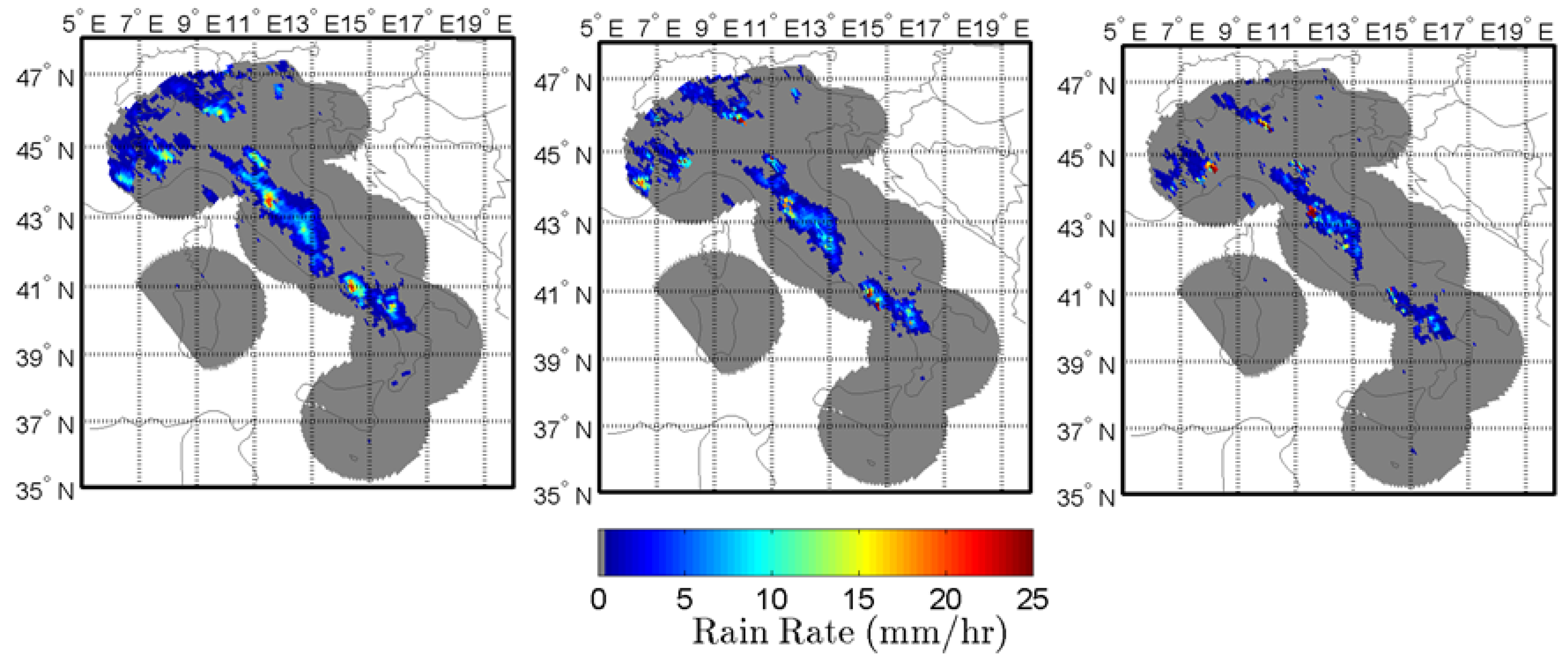
Figure 2 shows the precipitation patterns obtained by the RNC for different RNCI values and the pattern obtained by GPROF V05 with a precipitation threshold of 0.1 mm h
−1.
As RNCI increases, the rainfall region gets smaller and for RNCI = 4 it is more or less coincident with the area with a more distinct rainfall emission signal at 10 GHz (higher TBs). The GPROF V05 pattern obtained for a minimum threshold of 0.1 mm h
−1, results more similar to the PNPR v3 rainfall pattern obtained for RNCI ≥ 1. This example shows that, even if for RNC the best statistical scores globally are obtained for RNCI ≥ 2 (
Table 5), by providing all the RNCI values (0 to 4), PNPR v3 allows to adjust the rain/no rain pattern for specific cases and to perform analysis of the effect of RNC on the results.
6. Verification Study
An assessment of the final PNPR v3 retrieval has been carried out using the verification database (i.e., an independent part of the observational database, based on 2B-CMB V04 product, not used in the training and design phase of the algorithm, see
Section 3).
Figure 3 shows a pixel-based comparison of the surface rain rate estimates by PNPR v3 and the 2B-CMB, for vegetated and arid land, ocean and coast. Only pixels where both products provide rainfall rate ≥0.1 mm h
−1 (hits) were considered. Pixels with 2B-CMB liquid fraction <0.8, or with surface height greater than 2000 m, or with likely presence of ice or snow on the ground (according to the Snow Depth and Sea Ice Cover available from the ECMWF Era Interim re-analysis (0.125° × 0.125° resolution) have been also eliminated. Therefore, in the comparison liquid precipitation only is considered and cases that might likely be affected by larger uncertainty (in both products) are excluded. The figure shows a general good consistency between the two products, with a quite homogeneous trend in all the panels. Most of the points are close to the main diagonal for both vegetated land and ocean, with slight overestimation of very low precipitation (rain rates less than 1 mm h
−1), extending to moderate precipitation (rain rate up to 10 mm h
−1) mostly over ocean. A similar but less marked, trend is also found for arid land and coast.
The agreement between PNPR v3 and 2B-CMB points out the good outcome of the network training, as well as of its optimization and complex input selection procedure, allowing the use of one unique NN over the different surface types. PNPR v3, applied to an independent global dataset, with precipitation rates extending over a wide range of values (up to 80 mm h−1), shows a good ability to retrieve global precipitation without anomalous inhomogeneities in the estimates.
Table 6 shows the contingency table of PNPR v3 versus 2B-CMB. Each column represents the rain rate class for 2B-CMB, while each row represents the rain rate class for the PNPR v3. Four rainfall rate intervals were selected in this comparison, 0.1–1 mm h
−1, 1–10 mm h
−1, 10–30 mm h
−1 and ≥30 mm h
−1. The percentages shown in a given column, provided for the four surface types, represent how PNPR v3 classifies the precipitation assigned to the corresponding 2B-CMB class. There is a general consistency between PNPR v3 and 2B-CMB estimates, as shown by the largest percentages found on the main diagonal for each surface type. In the first column, corresponding to rain rate lower than 1 mm h
−1, where about 84–89% of hits are found (depending on the background surface), the agreement is particularly evident. Also for the second column the percentages of hits are fairly large, between 80% and 89%. For the third and fourth columns, corresponding to higher values of precipitation, the percentages on the main diagonal are lower, highlighting an underestimation (up to 44.5% of cases for vegetated land) and a maximum overestimation of 7.9% (arid land).
Table 7 shows the continuous statistical indexes calculated for the different surfaces (mean error (ME), mean absolute error (MAE), root mean square error (RMSE), standard deviation (SD), adjusted root mean square error (ARMSE) and correlation (CC)) obtained for PNPR v3 in the comparison with 2B-CMB estimates. The adjusted root mean square error is the RMSE corrected removing the bias [
67].
The table confirms the good agreement between the two products, with very low values of the errors (ME ranging from −0.22 to 0.10 mm h−1 and MAE from 0.60 to 0.94 mm h−1), low RMSE (less than 2.75 mm h−1) and a good correlation (≥0.90).
A further test on the performance of PNPR v3 was carried out by analysing the relative fractional standard error percentage (FSE%), that is, the ratio between RMSE and the mean “true” value, as a function of the 2B-CMB mean rainfall rate value computed for different rain rate intervals (0.5 mm h−1 bins):
Figure 4 shows a general agreement in the trends over the four surfaces. For precipitation rates lower than 1 mm h
−1, FSE% drops from 200 to 250% to values below 100% for all surface (with high FSE% for arid land and vegetated land). For rain rates between 1 and 10 mm h
−1, the FSE% varies for the different surface types between 80% and 40% (with overall better scores over ocean), while for higher rain rates FSE% does not vary much across the different surface types, ranging between 30% and 50%.
The results in the verification study were obtained using the same product (2B-CMB NS V04) used in the training phase of the algorithm, although for a completely independent dataset. It should be noted that, given the homogeneity of the (independent) verification database with the databases used in the training and design phase of the algorithm, good results on the performance of PNPR v3 were reasonably expected. In the next section two case studies over Italy are analysed, where ground-based radar precipitation estimates are used for comparison.
7. Case Studies
The first case study is a heavy rainfall storm that struck the Tuscany region, particularly the city of Livorno (Lat 43°32′N, Lon 10°19′E), between 9 and 10 September 2017. The convergence of a flow of warm, moist air of North Atlantic origin, from the Channel of Sicily towards the Tuscan archipelago with cooler winds from the west, gave rise to a condition of great instability, with heavy rainfall enhanced by the orography of the area.
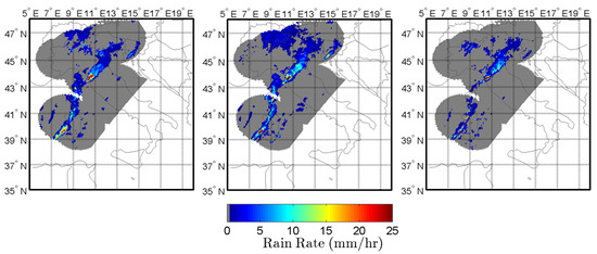
Figure 5 shows the PNPR v3 and GPROF V05 precipitation estimates for the GMI overpass on 10 September 2017 at 01:17 UTC, compared with quality-controlled rainfall rate estimates of national radar network mosaic (at 01:20 UTC), provided by the Department of Civil Protection of Italy, used as reference [
68].
In the figure, the PNPR v3 (left panel) and GPROF V05 (middle panel) precipitation estimates on the area covered by the Italian radar network are shown. Simultaneous radar observations (right panel) were averaged to match the nominal resolution of the corresponding satellite retrievals using a two-dimensional Gaussian function with an elliptic horizontal section (oriented considering the orientation of the satellite orbit with respect to the surface at the time of the overpass, see [
69] for details).
The minimum threshold for the GPROF rainfall rate has been set to 0.1 mm h
−1. Some differences in the rainfall patterns identified by the two GMI products can be noticed, with a larger extension of the GPROF light precipitation area. A good agreement between the two products and with respect to the radar is evident in the heavy precipitation areas (also around Livorno).
Table 8 shows the continuous statistical indexes evaluated for PNPR v3 and GPROF V05 compared with radar estimates (hits only). Both products tend to overestimate the precipitation (ME equal to 1.00 and 0.99 mm h
−1 for PNPR v3 and GPROF V05 respectively). The statistical scores are comparable but with differences in favour of the GPROF product.
Table 9 shows the dichotomous statistical scores for both PNPR v3 and GPROF V05 algorithms, with respect to the radar estimates. For PNPR v3 the statistical scores obtained considering the four different RNCI thresholds are shown. The results obtained confirm that the selection of the rain/no-rain pixels using RNCI ≥ 2 provides the best performance (according to the results showed in
Table 5). These results also confirm a good agreement in the pattern of the precipitation obtained by the two products, with a slightly better performance of PNPR v3 especially in terms of FAR.
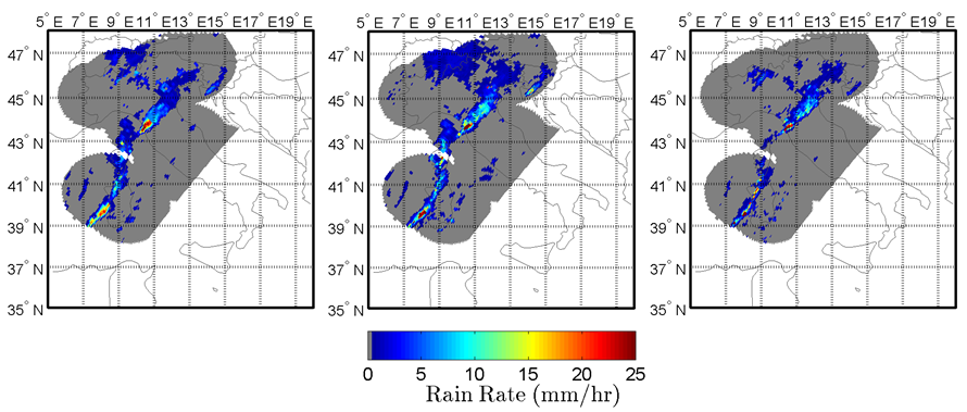
The second case study is a precipitation event that affected a large part of Italy, on 9 August 2015 and that produced some intense and complex rainfall pattern, with scattered limited areas of heavy rainfall (e.g., in Tuscany and Liguria region) and extended areas of light to moderate rainfall. This situation was entirely captured by a GMI overpass at 16:35 UTC (
Figure 6).
Also in this case there is a good agreement between the two products, showing very similar patterns and with respect to the radars, although PNPR v3 shows larger precipitation areas and overestimation of moderate precipitation.
Table 10 shows worse scores than the Livorno case, both for PNPR v3 and for GPROF V05, with larger overestimation (ME equal to 1.48 and 1.17 for PNPR v3 and GPROF V05 respectively). For this case, PNPR v3 shows higher correlation and lower RMSE than GPROF.
Table 11 confirms the good agreement in the pattern of the precipitation obtained by the two products, with a slightly better performance of PNPR v3 also for this case.
It has been evidenced by several authors [
70] that in a validation exercise spatial colocation and horizontal averaging of measurements (both ground-based and satellite-based) are key elements critically affecting the results. We want here to highlight that all the statistical scores in this study have been obtained using pixel-based comparison of instantaneous precipitation rate estimates. The good agreement with ground-based radars in terms of spatial pattern and statistical scores for both PNPRv3 and GPROF confirms the high quality of the two GMI-based algorithms.
8. Summary and Conclusions
In this work, a new algorithm based on the Passive microwave Neural network Precipitation Retrieval approach (PNPR v3), designed to work with the conically scanning GMI radiometer, is thoroughly described and results about its performance are presented and discussed. This algorithm, developed within the EUMETSAT H SAF program, follows the two previous PNPR (v1 and v2) products designed to work with cross-track scanning radiometers, AMSU/MHS and ATMS [
26] and [
27]. Although it benefits from the experience acquired with the development of the previous algorithms, this new version of PNPR presents several innovations with respect to the others.
A fundamental new aspect is that PNPR v3 is a global rainfall rate retrieval algorithm (between 65°N–S), while PNPR v1 and v2 algorithms are designed to work over the MSG full disk area, [60°S–75°N, 60°W–60°E]). As opposed to previous PNPR algorithms, based on a training database obtained from cloud-radiation model simulations, the new PNPR v3 for GMI is completely based on an extremely large observational database (with over 150 million elements with rainfall) built from coincident GMI/DPR global observations during a period of 27 months between 2014 and 2016. In the database, the NASA 2B-CMB V04 rainfall rate product (Normal Scan swath, liquid fraction >0.8) is used as reference. In addition, a new PCA-based input selection procedure has been designed to fully exploit the potentials of GMI channels compared to AMSU/MHS and ATMS. Another difference is a new rain/no-rain classification scheme (RNC), also based on the NN approach, which provides different rainfall masks for different minimum thresholds and degree of reliability. The procedure to design one unique NN for all surface types has been also described.
In order to assess the performance of PNPR v3 over the globe, an independent part of the observational database, composed of about 50 million data distributed globally in 27 months period, not used in the algorithm design phase, is used in a verification study. A good agreement is found between PNPR v3 and 2B-CMB products, with a good CC (greater than 0.90), very low values of the ME (between 0.10 and −0.22 mm h
−1), MAE (between 0.60 and 0.94 mm h
−1) and RMSE (between 1.62 and 2.75 mm h
−1). Also, the FSE% drops below 100% for rainfall rates lower than 1 mm h
−1, ranging around 30–50% for moderate to high rainfall rates, over all surface types. These good results, also compared to previous versions of PNPR v1 and v2 [
26,
27], or other studies [
67], besides demonstrating the good outcome of the input selection procedure, as well as of the training and design phase of the NN, also show how PNPR v3 is able exploit the great capabilities of GMI for rainfall retrieval over the different surface types. It is worth noting, however, that, since the algorithm has been trained for (mostly) liquid precipitation, ancillary variables indicating the possible occurrence of (mostly) frozen precipitation have been used in the PNPR v3 assessment to limit the verification to rainfall cases.
The further verification carried out on two case studies over Italy, showed a good consistency of PNPR v3 retrievals with GPROF V05 estimates and with simultaneous ground-based radar estimates. The dichotomous statistical indexes indicated good rainfall detection skills by PNPR v3 (FAR = 0.37 and 0.36, POD = 0.70 and 0.83 and HSS = 0.59 and 0.70 for the two cases), with consistently better scores than GPROF (especially the lower FAR), except for the higher POD for GPROF in one case. For the rainfall rate retrieval, the continuous statistical scores indicated slight overestimation by the two GMI products (with higher ME and MAE for PNPR v3 than for GPROF), while the other scores indicated better performance of PNPR v3 in one case and of GPROF for the other case. It is worth noticing the ability of PNPR v3 to provide rainfall rate estimates in agreement with the ground-based radar and with the well consolidated GPROF v05 product for these two cases, characterized by extremely variable precipitation intensity across different surface typologies and complex orography.
The new PNPR v3 is a global rainfall retrieval algorithm, able to optimally exploit the GMI multi-channel response to different surface types and precipitation structures found around the globe. The PCA-based input selection procedure, where the precipitation signal is separated from the signal related to the different surfaces types, with minimal use of model-derived ancillary parameters, as well as the training and optimization of one unique NN allow to: (1) handle the extremely rich database based on the GPM-CO measurements and products; (2) provide global rainfall retrieval in a computationally very efficient way, making the product suitable for near-real time operational applications; (3) avoid discontinuities across different background surfaces.
The approach can be easily adapted to new versions of GPM products as they become available (including high quality snowfall rate estimates), or to background surface conditions that have not been considered in this study (e.g., frozen soil, snow cover, sea ice). However, due to the limited sensitivity of GPM DPR to snowfall especially at higher latitudes, separate modules for snowfall detection and retrieval recently developed by Rysman et al. [
35] will be coupled to PNPR v3. These modules are based on the use of observational databases built from GMI and Cloudsat snowfall coincident observations [
37].
In the future, a more extensive independent validation of PNPR v3 precipitation rate product using ground-based radars and rain gauges will be carried out over Europe within the EUMETSAT HSAF program. Moreover, in order to evaluate the PNPR v3 globally and compare it to GPROF (the GPM official PMW product) a more exhaustive analysis of different case studies around the globe will be carried out within the ongoing scientific collaboration between the EUMETSAT HSAF and GPM, on precipitation algorithm development and validation.

 ,
, 


