Consideration of Radiometric Quantization Error in Satellite Sensor Cross-Calibration

1
Science Systems and Applications, Inc., 1 Enterprise Pkwy, Hampton, VA 23666, USA
2
NASA Langley Research Center, Hampton, VA 23666, USA
*
Author to whom correspondence should be addressed.
Remote Sens. 2018, 10(7), 1131; https://doi.org/10.3390/rs10071131
Submission received: 8 June 2018
/
Revised: 9 July 2018
/
Accepted: 9 July 2018
/
Published: 18 July 2018
Abstract
:The radiometric resolution of a satellite sensor refers to the smallest increment in the spectral radiance that can be detected by the imaging sensor. The fewer bits that are used for signal discretization, the larger the quantization error in the measured radiance. In satellite inter-calibration, a difference in radiometric resolution between a reference and a target sensor can induce a calibration bias, if not properly accounted for. The effect is greater for satellites with a quadratic count response, such as the Geostationary Meteorological Satellite-5 (GMS-5) visible imager, where the quantization difference can introduce non-linearity in the inter-comparison datasets, thereby affecting the cross-calibration slope and offset. This paper describes a simulation approach to highlight the importance of considering the radiometric quantization in cross-calibration and presents a correction method for mitigating its impact. The method, when applied to the cross-calibration of GMS-5 and Terra Moderate Resolution Imaging Spectroradiometer (MODIS) sensors, improved the absolute calibration accuracy of the GMS-5 imager. This was validated via radiometric inter-comparison of GMS-5 and Multifunction Transport Satellite-2 (MTSAT-2) imager top-of-atmosphere (TOA) measurements over deep convective clouds (DCC) and Badain Desert invariant targets. The radiometric bias between GMS-5 and MTSAT-2 was reduced from 1.9% to 0.5% for DCC, and from 7.7% to 2.3% for Badain using the proposed correction method.

1. Introduction
The purpose of radiometric calibration is to establish the quantitative relationship between the digital measurements, or raw counts, recorded by a satellite imaging system and the spectral radiance arriving at the imaging sensor. Accurate radiometric calibration is critical for all quantitative applications of remotely-sensed satellite data. Many present-day satellite imagers carry advanced calibration systems for on-orbit calibration. The Moderate Resolution Imaging Spectroradiometer (MODIS) instrument onboard the Aqua and Terra platforms, and Visible Infrared Imaging Radiometer Suite (VIIRS) on the National Polar-orbiting Partnership (NPP) satellite, have sophisticated onboard calibration systems, which utilize a solar diffuser (SD) and an SD stability monitor to perform in-flight radiometric calibration, as well as to monitor the long-term sensor stability [1]. For instruments without onboard calibrators, the radiometric calibration can be accomplished through a vicarious method, or cross-calibration. One approach of cross-calibration is using the coincident measurements from a reference instrument whose calibration is known. By comparing the raw counts from a target instrument (whose calibration is to be determined) with the calibrated radiances (provided by the reference instrument) that are coincident in time and identical in viewing and solar geometry, the radiometric calibration of the target instrument can be established. Such identical measurements from two satellite instruments are not feasible in reality as the two instruments always exhibit sampling differences that introduce an uncertainty in cross-calibration. Similarly, the instrumental differences (spectral, spatial, radiometric resolution, etc.) between the reference and target sensors can also affect the cross-calibration results [2,3].
The Clouds and Earth’s Radiant Energy System (CERES) project [4] at NASA implements “a common reference standard” policy to consistently calibrate the 16 geostationary Earth orbiting (GEO) visible imagers that are used to derive top-of-atmosphere (TOA) broadband fluxes and cloud properties to account for the regional diurnal fluctuations between the Terra and Aqua CERES and MODIS measurements [5]. Each of the 16 GEOs in the CERES Edition 4A (Ed4A) record derives its calibration via cross-calibration with Aqua-MODIS Collection 6 band 1 radiances (or Terra-MODIS band 1 radiances for GEOs that operated before the Aqua-MODIS record) using the all-sky tropical ocean ray-matching (ATO-RM) method [6,7]. The ATO-RM method utilizes the near-coincident, co-located, and co-angled GEO counts and MODIS radiance pairs located over ATO scenes to transfer the MODIS calibration to the GEO imager. The ray-matched datasets are gridded into larger footprints in order to mitigate any navigation uncertainty due to a spatial resolution difference between the two sensors. Similarly, CERES Ed4A implements scene-dependent spectral band adjustment factors (SBAF) to account for the spectral response function (SRF) differences between MODIS and GEO.
Another important instrumental characteristic that can introduce a systematic bias in the cross-calibration of GEO and MODIS is the difference in radiometric quantization, which is not accounted for in the CERES Ed4A GEO calibration. In satellite remote sensing, the radiometric quantization refers to the transform of the continuous Earth-reflected solar radiation reaching the satellite sensor into a finite number of digital counts. The more bits that are employed for quantization, the greater the sensitivity of the satellite imaging system for detecting small changes in the incoming radiance. Lowering the number of bits for quantization results in a larger quantization level, which impairs the radiometric quality of the satellite products. Data quantization for MODIS instruments is 12-bit. The majority of GEO imagers that operated during the CERES record (2000 to the present) implement 10-bit quantization. Because these 10-bit GEO imagers have a linear count response, and the ray-matched data pairs are gridded and averaged, it is assumed that the quantization difference may contribute additional noise to the monthly regression data, but should not bias the GEO calibration slope. It has been found, however, that the impact of quantization error in cross-calibration can be much larger for the visible and infrared spin scan radiometer (VISSR) onboard Geostationary Meteorological Satellite-5 (GMS-5), which has a 6-bit squared count sensor response (at-sensor radiance is proportional to squared raw count) [7].
For sensors with coarse radiometric resolution, it is important to take into account the quantization error (QE) when pixel-level counts or radiances are averaged into a larger area. This is crucial for the GMS-5 VISSR and MODIS ATO-RM cross-calibration, which relies on spatially averaged pixel-level counts and radiances. The objective of this paper is to describe a simulation approach for studying the impact of quantization differences in satellite cross-calibration, and highlight the need for considering the quantization errors for improving the cross-calibration results. Section 2.1 describes the CERES ED4A GMS-5 VISSR and MODIS inter-calibration technique and illustrates the impact of not accounting for the sensor quantization on the resulting GMS-5 calibration coefficients. The impact of quantization difference on the calibration of GMS-5 is non-linear with radiance, and is shown in Section 2.2. Section 2.3 highlights previous studies that have calibrated GMS-5-like sensors. Section 2.4 presents the simulation approach for analyzing the impact of the GMS-5 low-resolution quantization in its cross-calibration with MODIS. A simple correction method based on shifting the GMS-5 squared counts up by a ½ step size is proposed in Section 2.5 in order to mitigate the quantization effect. Section 3 applies the QE corrections to GMS-5 VISSR counts and presents the improved calibration results for this sensor. The results demonstrate that with appropriate handling of quantization noise, the absolute calibration accuracy of GMS-5 VISSR can not only be improved, but also the associated calibration uncertainty can be lowered. Conclusions are contained in Section 4.
2. Methodology
In order to compute or adjust the calibration of a target sensor to that of a reference instrument, cross-calibration requires comparison datasets acquired by the two instruments over a common target. The comparison datasets can be near-coincident, collocated, and co-angled, such as the method implemented by CERES for calibrating GEO imagers [6,7], or they can be completely non-coincident in time as in cross-calibration approaches that utilize Earth invariant targets (deserts, deep convective clouds, etc.) [8,9,10,11,12]. In all cases, the comparison between the reference and target sensor data is rarely performed at the satellite pixel level. Larger cross-calibration target areas are preferred in order to mitigate the effect of spatial mismatch caused by sensor spatial resolution differences, time discrepancies, and imperfect navigation. The quantization error computed for the individual satellite pixels is different than the aggregated quantization effect of a larger area.
2.1. GMS-5 Inter-Calibration with MODIS
The CERES project calibrates the GEO imagers using MODIS as the calibration reference employing the ATO-RM method [6,7]. The CERES Ed4A ATO-RM method utilizes pixel-level GEO counts and MODIS radiances that are averaged on a 0.5° latitude by 0.5° longitude grid located over all-sky tropical ocean scenes. The ray-matching observations are limited to within ±15° of the equator and ±20° in longitude from the sub-satellite point, and must be coincident within 15 min. The viewing and azimuthal angles are matched within 15°. The large gridded calibration footprints mitigate any navigation uncertainty (possibly caused by a spatial resolution difference), parallax errors, and mismatching caused by cloud advection [13]. The GEO imagers have SRFs that are much broader than that of MODIS band 1. CERES Ed4A implements spectral corrections, or SBAF, based on the SCanning Imaging Absorption spectrometer for Atmospheric CHartographY (SCIAMACHY) level-1b version-7.01 hyperspectral footprint radiances acquired over ATO scenes to eliminate any spectrally induced bias due to the SRF differences [2,7]. The spectrally corrected gridded MODIS radiances and GEO counts are regressed on a monthly basis in order to compute the GEO calibration gain, which is tracked over time to derive the temporal radiometric degradation of the GEO imaging sensor.
The VISSR onboard GMS-5 operated by Japan Meteorological Agency (JMA) is the only GEO imager during the CERES record that has a squared count sensor response and a native radiometric resolution of 6-bit (0, 1, 2, 3, …, 63) [14]. The Man computer Interactive Data Access System (McIDAS) servers [15], which are the source for all GEO data used in the CERES project, translates the GMS-5 data to 8-bit (0, 4, 8, 12, …, 252) by simple factor-of-four scaling. The linear regression of the GMS-5 8-bit squared counts and ray-matched MODIS radiances for May of 2000 is shown in Figure 1a. For a perfect ray-matched dataset, the regression x-offset (intercept) should give the GEO space count (SC) value, which is the satellite-recorded residual count for zero input radiance (viewing at space or the dark portion of the Earth).
Note that the regression reveals a negative x-offset (−767 in this case) for GMS-5. At first glance, it appears that the GMS-5 imager cannot measure a zero radiance. However, the SC of GMS-5 was found to be 0 based on satellite pixels covering the unlit portion of the Earth disc. Also, a careful examination of GMS-5 images near terminator regions, where solar zenith angles (SZA) are slightly less than 90°, the satellite records 0 count (See Figure 2). This behavior is understood as a consequence of the large discretization intervals in the GMS-5 raw counts resulting from its poor 6-bit radiometric resolution. These intervals prevent the GMS-5 imager from recording the positive radiances near the terminator regions. The 12-bit MODIS instrument can easily resolve radiances near zero as well as can have a range of radiances in between any two consecutive GMS-5 discretization levels.
2.2. GMS-5 Quantization Error Dependence on Radiance
Figure 1b illustrates how the large radiometric resolution difference affects the linear regression between the ray-matched MODIS and GMS-5 gridded data pairs. The green dashed line represents the true calibration slope of GMS-5. The GMS-5 measured radiance corresponding to a squared count of 64 is shown as y on the green dashed line. Because MODIS can resolve radiances between 64 and its next quantization level, which is 144, the average value of MODIS radiance pixels within the matching 0.5° latitude by 0.5° longitude grid will always be higher (somewhere in between the two consecutive squared count levels as represented by y’) than the expected value based on the dashed green line for the entire range of GMS-5 squared counts. A linear regression (solid red line) fit to the observed MODIS and GMS-5 ray-matched gridded pairs will lie above the true calibration slope of GMS-5, thereby resulting in a negative x-offset. For instruments with a linear count response, the discretization intervals are uniform, and therefore the x-offset tends to be near the −½ quantization step. For GMS-5, which has a quadratic relationship between radiance and count, the quantization step is smaller for lower radiances and becomes greater with increasing input radiance. The value of the x-offset then depends on the distribution of the monthly ray-matched data along the dynamic range. The gridded data points near the higher end of the dynamic range have a tendency to result in a larger magnitude of x-offset. This will be discussed in more detail in Section 2.4.
Because of this varying discretization step size, the magnitude of QE is different at different radiance levels, thereby introducing a non-linearity in the regression data pairs. The regression slope and offset will therefore change depending upon the distribution of the data along the dynamic range. This can be understood better with a hypothetical illustration shown in Figure 3. The x-axis of Figure 3a represents the 64 discretization levels of GMS-5 6-bit counts that are scaled to 8-bit and squared. The blue points are true GMS-5 measured radiances corresponding to these squared count levels, assuming that GMS-5 has 0 SC and a calibration slope of 0.0625 (chosen arbitrarily). The y-axis represents the reference radiance with a much higher quantization resolution than that of GMS-5. For ray-matched gridded data pairs, the matched reference radiance for a gridded GMS-5 squared count is close to 0.0625 × (Count2 + ½ step size), assuming that the scene conditions within the 0.5° grids are fairly uniform. The red points in Figure 3a represent the estimated reference radiances computed by adding an offset radiance equivalent to ½ step size of GMS-5. Because the step size varies along the dynamic range, the curve joining the red points must be non-linear. The slope of the red curve is computed at each point and is shown in Figure 3c. At lower radiance values, the slope is much steeper (highlighted in Figure 3b), and further away from the true calibration slope of GMS-5. On the other hand, the brighter radiances tend to lower the slope of regression, bringing the slope closer to the actual calibration slope.
2.3. Historical VISSR Calibration Efforts
Although QE might seem straightforward to correct, it has often been disregarded. Fraser and Kaufman (1986) remarked that the QE in the Geostationary Operational Environmental Satellites (GOES) VISSR imagers were negligible compared to the uncertainties due to detector-to-detector calibration differences, sub-pixel clouds, and radiative transfer model radiances [16]. Also, the VISSR analog-to-digital converter (ADC) on GOES-5 did not perfectly convert the photo multiplier tubes signal into a 6-bit squared count, thereby contributing to a 7% error in the radiance [17]. Therefore, due to other severe hardware issues in the earlier satellite instruments, these studies did not address the QE. The calibration stability of the GMS-5 VIISR imager, launched in 1995, was improved by replacing the photomultiplier tubes with silicon photo diodes [18,19]. Le Marshal et al. [20] inter-calibrated GMS-5 VIISR and National Oceanic and Atmospheric Administration (NOAA)-14 Advanced Very High-Resolution Radiometer (AVHRR) by ray matching over carefully selected optically thick clouds. Their work used a linear regression forced through the space offset of both instruments and limited the comparison data to very bright and uniform count target areas, which accounted for QE. Minnis et al. [21] also used a linear regression forced through the observed space count in order to inter-calibrate GOES-7 VISSR with the NOAA-11 AVHRR imager.
The QE was probably not considered for later calibration studies because the recent imagers have a much greater radiometric resolution and linear sensor response. The QE of the VISSR imagers for these later calibration studies were more than likely overlooked. Nguyen et al. calibrated GMS-5 with the Visible and Infrared Scanner (VIRS) instrument onboard Tropical Rainfall Measuring Mission (TRMM) using grid-averaged ray-matched radiance pairs and noted a negative SC of –900 Count2 (Table 2 in [22]). Similarly, using 0.5° gridded TRMM-VIRS and GMS-5 ray-matched pairs, the linear regression intercept was found to be negative, prompting Minnis et al. to note that GMS-5 could not measure a zero radiance [23]. Inamdar and Knapp [24] calibrated the suite of International Satellite Cloud Climatology Project (ISCCP) GEO imagers using 50-km grid-averaged AVHRR and GEO data pairs. Most of the calibration offsets (a0 in Table 1 in Reference [24]) are positive for the VISSR imagers onboard GOES-1 through 7 and GMS-1 through 5. A positive offset in this case indicates a negative SC. The other GEO imagers that have a linear sensor response show negative offsets (positive SC). As stated previously, the CERES Ed4 GMS-5 calibration is biased because the QE has not been taken into account.
Ignatov et al. [25] cautions against using linear regression with an unconstrained intercept to determine the SC. Specifying the SC improves the accuracy of the calibration gain, especially for low radiances. The observed impact of the GMS-5 VISSR imager QE on the linear regression offset of the ray-matched data pairs supports an argument to not determine the imager SC using the linear regression intercept, but rather to use a linear regression forced through the SC.
Another imager example of the QE caused by the averaging of pixel-level counts based on a nonlinear sensor response, is the AVHRR-3 imager onboard the NOAA-15 through 19 satellites. The AVHRR-3 imager has a dual-gain response. The lower third of the radiance range has a gain factor of 3 times that of the upper 2/3 range. The nominal AVHRR pixel-resolution is 1.1-km. The global area coverage (GAC) data-set, however, uses averaged 4-pixel counts out of 15 to represent a 3 × 5-km footprint, and does not account for the dual gain nature of the sensor. Doelling et al. [26] reported that the GAC QE affected both the slope and intercept of the linear regression between the AVHRR and MODIS SNO matches. The impact of the QE on AVHRR calibration was mitigated by using a linear regression forced through the SC, and by using a spatial homogeneity filter to reduce the number of GAC footprints containing both low and high gain 1-km pixel counts [26].
2.4. Simulation Method
A simulation method is presented here to estimate the effect of quantization noise in the cross-calibration method that utilizes spatial averaging of pixels over a larger area. The simulation analysis was formulated using one 6-min granule (NPP_VIMD_SS.GRD.A2017014.2330.001.2017015100106.hdf) of the NPP-VIIRS L1B radiance product downloaded from the NASA Langley Atmospheric Science Data Center Distributed Active Archive Center (ASDC DAAC). The granule was located over the tropical Pacific Ocean in order to obtain a complex radiance field that encompassed the entire range of Earth-viewed radiances (see Figure 4). The 12-bit radiances acquired in the M5 band (0.65 μm) were resampled and quantized to lower-bit resolution counts using the following approach: First, the maximum value (Rmax) of the M5 pixel radiance was found to be 627.5 Wm−2 μm−1 sr−1 in the selected granule. Next, the analog to digital conversion resolution (ADCres) was determined for the desired bit count (n) representation using the following equation:
ADCres = Rmax/(2n ‒ 1)
For an n-bit satellite count with a linear response, the conversion of a VIIRS M5 radiance pixels (R) to counts was performed as follows:
Count = Integer(R/ADCres)
Similarly, for an n-bit squared count response, Equations (1) and (2) were modified as follows:
ADCres = √Rmax/(2n ‒ 1)
Count = Integer(√R/ADCres)
Count = Integer(√R/ADCres)
The VIIRS radiance and count image data were then gridded in 0.5° × 0.5° bins in order to derive a simulated version of the ATO-RM dataset. The mean was computed for all bins in terms of both the VIIRS radiance and the simulated count units. For squared count response, the counts were summed in quadrature before computing means. This process formed an ideal dataset for ATO-RM-based cross-calibration, where the binned radiance and count pairs were nearly perfectly matched in wavelength, angle, time, and space. A linear regression of the simulated bin counts against the bin radiances then allowed for the investigation of the sole effect of the discretization interval differences on the inter-calibration results.
2.4.1. Linear Sensor Response
Figure 5 shows the regression plots of the gridded VIIRS radiances (y-axis) and simulated counts (x-axis) for four different cases. Figure 5a,b illustrates the regression analysis for 8-bit and 6-bit satellite counts with a linear sensor response, respectively. In both cases, the y-offset was positive, suggesting a positive VIIRS radiance for 0 satellite count, a behavior similar to what has been seen with GMS-5 to MODIS ATO-RM. This radiance/count relationship was the outcome of regressing the higher radiometric resolution (12-bit in this case) VIIRS radiances against the downgraded discretization raw counts. The positive y-offset caused a negative x-offset. For sensors with a linear response, where the discretization count interval was always 1 count, the maximum value of QE on a pixel level could be anywhere between 0 and 1 count. For gridded datasets, the hypothetical experiment described in Section 2.2 followed the assumption that the scene conditions within the 0.5° × 0.5° grids were uniform such that the variation of MODIS pixel radiance values was confined to within one discretization level of GMS-5, thereby resulting in a grid-average value near the middle of two consecutive GMS-5 discretization levels. In reality, this assumption might not have held, meaning a 0.5° × 0.5° grid from the simulated VIIRS dataset may have contained pixel radiance values that fell into multiple discretization intervals along the dynamic range of GMS-5. The fact, however, that VIIRS could resolve one discretization interval of GMS-5 into 64 levels, and the assumption that 0.5° × 0.5° binning of the 1-km VIIRS data offered adequate random distribution of pixel radiance, still allowed the grid-average radiance value from VIIRS to be positioned close to the mid-value of the two consecutive discretization levels. The x-offset of −0.5 and −0.52 count in Figure 5a,b, respectively, supported this argument. The statistics in Figure 5a,b suggested that the standard error of linear regression for 8-bit representation had been reduced by 85% compared to that for the 6-bit. For sensors with a linear count-radiance relationship, ½ quantization level was always the same across the dynamic range, and therefore, adding 0.5 count to the native raw counts could help eliminate the negative x-offset in cross-calibration.
2.4.2. Squared Sensor Response
The regressions for simulated 6-bit squared count and 6-bit scaled to 8-bit squared count datasets are shown in Figure 5c,d, respectively. Figure 5d represents the case of GMS-5 data from McIDAS that rescaled the native 6-bit resolution of GMS-5 to 8-bit by a simple multiplication of 4. Scaling the 6-bit squared counts to 8-bit squared counts resulted in an x-offset (−156.65 in Figure 5d) that was 16 times the x-offset in Figure 5c. Unlike the previous two linear cases (Figure 5a,b), the discretization interval of the squared counts was not uniform and the step size increased with increasing count value. For example, the discretization of 6-bit squared count went as such: 0, 1, 4, 9, 16, 25, …, 3969. When it was scaled to an 8-bit squared count, the discretization levels were 0, 16, 64, 144, 256, …, 63,504. The step size, which was the difference between two consecutive squared counts, increased with the count. The relative QE, however, was larger for low squared counts because of the lower radiance value.
In order to illustrate how the linearly regressed slope and offset were dependent on the count or radiance value, the simulation dataset used in Figure 5d was divided into three subsets of varying radiance ranges: 0–50, 100–300, and >400 Wm−2 μm−1 sr−1. As such, the discrete ranges represented three different scene types with varying reflectance. The linear regression was now performed with the individual subsets as shown in Figure 6. The results showed that the brighter radiances provided a lower calibration slope, as well as a much larger magnitude of x-offset, as discussed above. This result was consistent with what was described earlier for the GMS-5 calibration using MODIS as a reference (Figure 1a). If the ray-matched MODIS radiances and GMS-5 counts were limited to bright deep convective clouds (DCC) pixels (Figure 6c), the resulting x-offset was found to be much larger than that of ATO-RM.
2.5. Half-Step Offset Correction
A correction method based on the adjustment of the raw counts of a target sensor with inferior radiometric resolution was proposed in order to mitigate the effect of QE in cross-calibration. The correction method was based on the assumption that the reference radiances in cross-calibration datasets were offset higher by an amount that was, on average, approximately equivalent to the radiance value corresponding to ½ the discretization step size of the target sensor. This assumption held fairly true for cross-calibration approaches, such as ATO-RM, where the comparison datasets were gridded over larger footprints and the complex scene conditions within the grids were avoided using a spatial homogeneity filter [6]. This offset in the reference radiance could be, therefore, compensated for by adding a ½ quantization level to the target sensor pixel count. For a squared count sensor, the discretization step sizes increased with counts. Figure 7a shows the quantization steps for 6-bit GMS-5 counts that were scaled to 8-bit and squared. The smallest and largest step sizes of GMS-5 8-bit squared counts were 16 and 2032 Count2, corresponding to the native 6-bit counts 0 and 63, respectively. The relative QE in the measurement of radiance or reflectance was higher at lower counts where the signal strength was low.
Figure 7b shows the regression of the same data as shown in Figure 5d after adjusting the pixel counts by a ½ quantization step size before binning. The new regression slope (0.0099) was lowered by ~2% and the new x-offset (5.54) was closer to zero (before it was −156.65). The standard error of regression was reduced by 40%, which was the result of reduced non-linearity in the new regression datasets. The new calibration slope was the same as in Figure 6c, where the regression data was limited to bright radiances (>400 Wm−2 μm−1 sr−1). The hypothetical example illustrated in Figure 3b had shown that the cross-calibration comparison using observations near the higher end of the dynamic range resulted in a more accurate calibration slope. Based on these arguments, it could be concluded that the proposed half-step offset (HSO) correction method could not only bring the x-offset closer to the true SC of the target sensor, but also improve the accuracy of its calibration slope. The residual x-offset of 5.54 was assumed to be owed to the imperfect assumption that the sample size within the ray-matched grids were adequate and uniform in order to yield a consistent HSO in average radiance values for the entire dynamic range. The same effect was also observed with the real GMS-5 data and will be discussed in Section 3.
After HSO correction, the resulting calibration slope and offset were found to be less dependent upon the dynamic range of the cross-calibration dataset, as illustrated in Figure 8. The dependence of the force-fit slope (left panel) and x-offset (right panel) upon the upper limit of the dynamic range for before and after HSO correction are shown in the top and bottom rows, respectively. Before correction, the calibration slope and offset were found near 0.0104 Wm−2 μm−1 sr−1/Count2 and −125 Count2, respectively, when limiting the brightness of the cross-calibration targets to radiances less than 100 Wm−2 μm−1 sr−1. When the cross-calibration dynamic range was increased to 600 Wm−2 μm−1 sr−1, the force slope reduced by 2.24% (Figure 8a) and the negative x-offset increased in magnitude by ≈34 Count2 (Figure 8b). For the HSO-corrected cross-calibration, the slope and offset remained fairly stable over the entire dynamic range, with the maximum variation of 0.07% for the slope (Figure 8c) and ≈1 count for the x-offset (Figure 8d).
3. Results and Discussion
3.1. GMS-5 HSO Validation
The HSO correction method described in the previous section was implemented to the measured GMS-5 visible counts from McIDAS, and its calibration was re-derived using the ATO-RM with Terra-MODIS C6 band 1 radiances during May 2000. The GMS-5 1.25-km spatial resolution raw pixel squared counts were adjusted for QE by adding a ½ quantization step prior to averaging within the grids. The CERES Ed4A GEO calibration relied on GMS-5 counts that were sub-sampled to 5-km data by sub-sampling in line and element to match the resolution of infrared (IR) pixels. Sub-sampling resulted in the loss of spatial information that was important for effective QE correction using the proposed HSO method. By just switching from the sub-sampled 5-km to the native 1.25-km GMS-5 resolution, the x-offset in Figure 1a was reduced from −767 Count2 to −242 Count2 (not shown). After the HSO correction, the regression x-offset was reduced to −32 (Figure 9a), closer to the space count value of 0. The residual offset was attributed to the added noise in the regression data pairs due to time matching differences between MODIS and GMS-5 acquisitions, tolerances in angular matching, spatial inhomogeneity, and residual QE. The May 2000 standard error of regression was reduced by ≈30% from 5.04% (Figure 1a) to 3.62% (Figure 9a), which suggested that the MODIS and GMS-5 ray-matched datasets exhibited a better linear relationship compared to the points in Figure 1a.
A new time series of GMS-5 visible imager calibration gain was computed for the HSO-corrected GMS-5 data using a force fit through SC = 0 (FFHSO(0)). The monthly gains are shown in Figure 9b with green squares, along with a linear fit to the points. The solid red line is the GMS-5 gain trend used in the CERES Ed4A products (without HSO), and was derived using SC = −650 Count2 (FF(−650)). For GMS-5 (without HSO), the average value of the monthly x-offset was found to be near −650 Count2 (not shown). The mean FFHSO(0) calibration gain after HSO correction was lower by 1.6% as compared to that of FF(−650) (Figure 9b). This was consistent with what was discussed earlier. That is, the QE produced an overestimate of calibration slope in ATO-RM. Furthermore, the temporal standard error was reduced by 25% (Figure 9b) when employing HSO. The monthly radiance dynamic range was not constant with time across the GMS-5 domain due to seasonal cloud pattern shifts, and therefore, the FF(−650) gains exhibited a greater seasonal variation than those of FFHSO(0). Because the CERES Ed4A used a constant negative space count, whereas the new HSO-correction-based GMS-5 gains used a dynamic offset, the radiometric bias between the two sets of GMS-5 gains varied with the magnitude of spectral radiance being measured. This effect is depicted in Figure 10. The x-axis showed the range of 6-bit GMS-5 raw counts, and the right-side y-axis represents the spectral radiance corresponding to these counts. The two sets of GMS-5 calibration curves are shown along with a difference line (red curve). The y-axis for the difference curve is shown on left side. The comparison shows that the expected difference between the two calibrations was reduced at the higher end of the dynamic range, i.e., measurements over bright clouds. The difference became much larger for darker radiances. For bright targets with an at-sensor spectral radiance greater than 100 Wm−2 μm−1 sr−1, the difference was less than 3%. Figure 10 also revealed that FF(−650) could significantly overestimate the radiance for darker targets like vegetation and ocean.
3.2. GMS-5 and MTSAT-2 Comparison
The improvement in the absolute accuracy of GMS-5 calibration after the HSO correction was evaluated by comparing the GMS-5 TOA responses over two Earth invariant targets, namely tropical DCC and the Badain Jaran Desert, with those from the visible imager onboard Multifunctional Transport Satellite-2 (MTSAT-2). If the FFHSO(0) method was an improvement over FF(−650), then the DCC and desert reflectances between GMS-5 and MTSAT-2 should have been more consistent. The MTSAT-2 imager had a 10-bit radiometric resolution and a linear count response; thereby it was minimally impacted by QE. The DCC and desert targets were considered to be pseudo invariant calibration sites (PICS), meaning they should have had about the same reflectance during both the GMS-5 and MTSAT-2 time periods. Because MTSAT-2 was located approximately at the same equatorial longitude position as GMS-5, and employed nearly the same imaging schedule, the two instruments sampled similar DCC conditions over the Tropical Western Pacific (TWP), and also observed the Badain desert with similar viewing and solar conditions. For the comparison study, both the GMS-5 and MTSAT-2 imager radiances were calibrated using the ATO-RM with MODIS, and were therefore on the same radiometric scale. For both the DCC and Badain desert targets, the spectral differences between GMS-5 and MTSAT-2 were accounted for by adjusting the GMS-5 radiances and reflectances to equivalent MTSAT-2 measurements using NASA-Langley’s SCIAMACHY-based spectral difference correction tool [2,27].
3.2.1. Deep Convective Clouds
The DCC response comparison between GMS-5 and MTSAT-2 was performed using the DCC-mode invariant target method as described in the Global Space-based Inter-Calibration System (GSICS) ATBD [12] and previous works [7,28], and is briefly described here. For both GMS-5 and MTSAT-2, DCC pixels over the TWP domain (±20° in latitude and longitude from the geostationary sub-satellite point) were identified using an infrared brightness temperature (IR-BT) < 205 K threshold. The viewing and solar zenith angles were limited to 40° in order to capture the more Lambertian part of the DCC reflectance. Homogeneity filters based on the standard deviation of the surrounding 3 by 3 block of pixels were applied to the IR-BT measurements and the visible radiance values in order to capture the DCC cores and eliminate any cloud edges. If the IR-BT and visible standard deviations were less than 1 K and 3%, respectively, the center pixel was identified as a DCC core. The valid DCC pixels were corrected to nadir conditions using the Hu DCC bidirectional reflectance distribution function (BRDF) [29]. The BRDF-corrected DCC pixel radiances were then compiled into monthly probability distribution functions (PDFs). The mode of the monthly PDFs was found to be stable to within 0.5% for visible channels as reported in previous studies [12,30]. For the GMS-5 and MTSAT-2 comparison, the monthly DCC mode radiances were averaged over the 3-year and 5-year records, respectively, as shown in Figure 11a. The results showed that the mean GMS-5 FF(−650) DCC response was 1.9% greater than the MTSAT-2 DCC response. The similar difference of 2% between GMS-5 FF(−650) and MTSAT-2 DCC mode radiances was also reported by Doelling et al. (Figure 12 in Reference [12]). This difference was reduced to 0.5% using the GMS-5 FFHSO(0) gains.
3.2.2. Badain Jaran Desert
The Badain Jaran Desert is located in central Inner Mongolia of Northern China, and is reported to be the most invariant site within the GEO domain of GMS-5 [31]. Bhatt et al. reported that the long-term temporal stability of the combined desert surface reflectance and the atmospheric column above it is less than 2% based on the 11 years of Aqua-MODIS band 1 observations [10]. Similarly, the inter-annual variability in the desert TOA radiances caused by any seasonal cycle of aerosols and water vapor is also found to be less than 2% [7]. A 0.4° × 0.4° squared region-of-interest (ROI) centered at 40.1°N latitude and 101.8°E longitude was selected over Badain. The desert ROI was viewed by GMS-5 and MTSAT-2 with a viewing zenith angle (VZA) of ≈61° and 64°, respectively. The 3° difference in VZA was the result of slight disparity in the sub-satellite points of GMS-5 (located at 140°E) and MTSAT-2 (located at 145°E). Because the Badain Jaran Desert is located at a higher latitude compared to most desert PICS, it was viewed by GMS-5 at a relatively large VZA, and thus the desert TOA reflectance exhibited a large seasonal cycle. The Badain Jaran Desert reflectance was much lower compared to that of DCC. This low reflectance allowed for performance evaluation of the HSO-corrected GMS-5 gains at the mid to lower end of the dynamic range. Because of the annually repeating imaging schedules of the two GEOs, their TOA reflectances over the Badain Jaran Desert could be compared on a daily basis. For maximum signal-to-noise-ratio, the local noon image for the desert site was selected every day. Clear-sky conditions over the desert were identified based on a spatial homogeneity test [10]. At near local noon, the SZA over the Badain Jaran Desert was found to vary from 18° in summer to 63° during winter. Therefore, the satellite-measured spectral radiances were higher during the summer than during the winter months.
The comparison of daily TOA reflectances between GMS-5 and MTSAT-2 is shown in Figure 11b. It is known that the desert surface reflectance increases with SZA [32]. The mean TOA reflectance bias between GMS-5 FF(−650) (red diamonds) and MTSAT-2 (blue diamonds) was found to be 7.7%, with GMS-5 being higher. The difference was larger during winter months when the solar illumination over the Badain Jaran Desert decreased, resulting in much lower values of satellite-measured counts. This was consistent with Figure 10, in that the use of the constant negative SC for GMS-5 introduced larger QE at the lower end of the sensor dynamic range. The FFHSO(0) calibration is shown with black diamonds. The mean of these reflectance values agreed with MTSAT-2 measurements within 2.3%, which was a significant reduction in the radiometric bias between the two instruments. The remaining 2.3% bias could be attributed to the desert VZA difference observed by GMS-5 and MTSAT-2. A kernel-driven BRDF model of the Badain Jaran Desert based on Aqua-MODIS band 1 reflectance data showed that the desert reflectance decreased by ≈1% when changing the VZA from 61° to 64° at an SZA of 20° [33]. The estimated BRDF difference was found to be ≈3% when the SZA was increased to 60°.
The HSO correction method, therefore, resulted in a linear calibration of GMS-5 that provided a consistent conversion of GMS-5 squared counts to radiance or reflectance units across the entire dynamic range, as demonstrated by looking at DCC and desert targets.
4. Conclusions
In satellite-based remote sensing, the number of digital bits used for radiometric quantization of the onboard imaging sensor determines the discretization interval that is directly associated with the sensor’s ability to detect incremental reflectance differences. Historical satellite imagers, such as GMS-5, used a lower bit-rate for quantization to help reduce the data volume of satellite images at a cost of reduced radiometric resolution. In order to retrieve uniform GEO cloud properties and surface fluxes, the CERES project inter-calibrates all GEO imagers using MODIS as a common reference based on coincident ray-matched pairs. Because the ray-matched pairs are obtained from pixel count averages over a 0.5° × 0.5° latitude by longitude grid, the cross-calibration between MODIS and GMS-5 is impaired by the large quantization difference between the two instruments. In fact, whenever GMS-5 pixel counts are averaged over a spatial domain, the quantization error has to be accounted for. The GMS-5 sensor has 6-bit radiometric resolution, which is much coarser than the 12-bit MODIS sensor, and possesses a quadratic relationship between counts and radiance by design. The large difference in the quantization resolution and the squared count feature of GMS-5 resulted in a biased calibration slope and a negative SC = −650 Count2 for GMS-5. Because many historical calibration studies did not factor in quantization error, it was important to document the impact on the calibration coefficients and provide solutions to mitigate the error.
This paper presented a simulation methodology for analyzing the impact of QE in satellite cross-calibration for both linear- and square-count response sensors. For linear-response sensors, the effect of QE could be mitigated by simply adding 0.5 count to the binned raw counts prior to regression. The simulation results satisfactorily explained the cause of the negative space count for GMS-5 based on the non-linearity introduced by QE in the cross-calibration datasets. A HSO correction method was also presented, in which the simulated squared counts of GMS-5 were adjusted prior to cross-calibration with the reference radiances. Because of the squared count response, the discretization intervals of GMS-5 were not uniform. The HSO correction proposed to add a ½ discretization step size to the squared counts in order to mitigate the effect of QE in cross-calibration. The simulation for the HSO correction method showed that the non-linearity in the cross-calibration dataset was mostly removed and the new GMS-5 SC tended to 0.
The recommended HSO correction was applied to the CERES GMS-5 and Terra-MODIS coincident ray-matched dataset. The results demonstrated that the linearly regressed intercept was very close to the observed SC of 0. In addition to incorporating the HSO, using a linear regression through the observed SC while only matching the more spatially uniform count pairs improved the overall absolute radiometric accuracy. This effect was validated using the DCC and Badain desert Earth-invariant targets. The radiometric bias between GMS-5 and MTSAT-2 DCC radiances, where both GEO imagers were inter-calibrated using the MODIS calibration reference, was reduced from 1.9% to 0.5% by applying the HSO correction. Similarly, the mean TOA GMS-5 and MTSAT-2 Badain desert reflectances were reduced from 7.7% to 2.3% using the improved gains for GMS-5. These results confirmed that the HSO-corrected GMS-5 squared counts were linearly proportional to ray-matched MODIS radiances, and that the data pair regression intersect was close to the SC of 0.
Author Contributions
R.B. and D.D. formulated the simulation methodology and analyzed the results. C.H. generated the simulation data and processed the MTSAT-2 and GMS-5 calibration using ATO-RM. B.S. and A.G. derived the spectral corrections for the sensors used in this study. All authors contributed to the preparation and revision of the manuscript.
Acknowledgments
This work was supported by the National Aeronautics and Space Administration Earth (NASA) Science Enterprise Office through the CERES and Research Announcement (NRA) NNH15ZDA001N, Research Opportunities in Space and Earth Science (ROSES-2015), and Program Element A.34: Satellite Calibration Interconsistency Studies.
Conflicts of Interest
The authors declare no conflict of interest.
Glossary of Acronyms
| ADC | Analog-to-Digital Converter |
| ASDC | Atmospheric Science Data Center |
| ATO-RM | All-sky Tropical Ocean Ray Matching |
| AVHRR | Advanced Very High-Resolution Radiometer |
| BRDF | Bidirectional Reflectance Distribution Function |
| CERES | Clouds and Earth’s Radiant Energy System |
| DAAC | Distributed Active Archive Center |
| DCC | Deep Convective Clouds |
| FF | Force Fit |
| GAC | Global Area Coverage |
| GEO | Geostationary Earth Orbiting |
| GMS-5 | Geostationary Meteorological Satellite-5 |
| GSICS | Global Space-based Inter-Calibration System |
| HSO | Half-Step Offset |
| IR-BT | Infrared Brightness Temperature |
| ISCCP | International Satellite Cloud Climatology Project |
| JMA | Japanese Meteorological Agency |
| McIDAS | Man computer Interactive Data Access System |
| MODIS | Moderate Resolution Imaging Spectroradiometer |
| MTSAT-2 | Multifunction Transport Satellite-2 |
| NASA | National Aeronautics and Space Administration |
| NOAA | National Oceanic and Atmospheric Administration |
| NPP | National Polar-orbiting Partnership |
| Probability Distribution Function | |
| PICS | Pseudo-Invariant Calibration Site |
| QE | Quantization Error |
| ROI | Region of Interest |
| SBAF | Spectral Band Adjustment Factors |
| SC | Space Count |
| SCIAMACHY | SCanning Imaging Absorption spectrometer for Atmospheric CHartographY |
| SRF | Spectral Response Function |
| SZA | Solar Zenith Angle |
| TOA | Top of Atmosphere |
| TRMM | Tropical Rainfall Measuring Mission |
| TWP | Tropical Western Pacific |
| VIIRS | Visible Infrared Imaging Radiometer Suite |
| VIRS | Visible and Infrared Scanner |
| VISSR | Visible and Infrared Spin Scan Radiometer |
| VZA | Viewing Zenith Angle |
References
- Xiong, X.; Angal, A.; Butler, J.; Cao, C.; Doelling, D.R.; Wu, A.; Wu, X. Global Space-based Inter-Calibration System Reflective Solar Calibration Reference: From Aqua MODIS to S-NPP VIIRS. Proc. SPIE 2016, 9881. [Google Scholar] [CrossRef]
- Scarino, B.R.; Doelling, D.R.; Minnis, P.; Gopalan, A.; Chee, T.; Bhatt, R.; Lukashin, C.; Haney, C.O. A web-based tool for calculating spectral band difference adjustment factors derived from SCIAMACHY hyperspectral data. IEEE Trans. Geosci. Remote Sens. 2016, 54, 2529–2542. [Google Scholar] [CrossRef]
- Chander, G.; Hewison, T.J.; Fox, N.; Wu, X.; Xiong, X.; Blackwell, W.J. Overview of Intercalibration of Satellite Instruments. IEEE Trans. Geosci. Remote Sens. 2013, 51, 1056–1080. [Google Scholar] [CrossRef]
- Wielicki, B.A.; Barkstrom, B.R.; Harrison, E.F.; Lee, R.B., III; Smith, G.L.; Cooper, J.E. Clouds and the Earth’s Radiant Energy System (CERES): An Earth Observing System experiment. Bull. Am. Meteorol. Soc. 1996, 77, 853–868. [Google Scholar] [CrossRef]
- Doelling, D.R.; Loeb, N.G.; Keyes, D.F.; Nordeen, M.L.; Morstad, D.; Nguyen, C.; Wielicki, B.A.; Young, D.F.; Sun, M. Geostationary enhanced temporal interpolation for CERES flux products. J. Atmos. Ocean. Technol. 2013, 30, 1072–1090. [Google Scholar] [CrossRef]
- Doelling, D.R.; Haney, C.O.; Scarino, B.R.; Gopalan, A.; Bhatt, R. Improvements to the geostationary visible imager ray-matching calibration algorithm for CERES Edition 4. J. Atmos. Ocean. Technol. 2016, 33, 2679–2698. [Google Scholar] [CrossRef]
- Doelling, D.; Haney, C.; Bhatt, R.; Scarino, B.; Gopalan, A. Geostationary Visible Imager Calibration for the CERES SYN1deg Edition 4 Product. Remote Sens. 2018, 10, 288. [Google Scholar] [CrossRef]
- Uprety, S.; Cao, C. Suomi NPP VIIRS reflective solar band on-orbit radiometric stability and accuracy assessment using desert and Antarctica Dome C sites. Remote Sens. Environ. 2015, 166, 106–115. [Google Scholar] [CrossRef]
- Mishra, N.; Helder, D.; Angal, A.; Choi, J.; Xiong, X. Absolute Calibration of Optical Satellite Sensors Using Libya 4 Pseudo Invariant Calibration Site. Remote Sens. 2014, 6, 1327–1346. [Google Scholar] [CrossRef] [Green Version]
- Bhatt, R.; Doelling, D.R.; Morstad, D.; Scarino, B.R.; Gopalan, A. Desert-based absolute calibration of successive geostationary visible sensors using a daily exoatmospheric radiance model. IEEE Trans. Geosci. Remote Sens. 2014, 52, 3670–3682. [Google Scholar] [CrossRef]
- Bhatt, R.; Doelling, D.R.; Scarino, B.R.; Gopalan, A.; Haney, C.O.; Minnis, P.; Bedka, K.M. A consistent AVHRR visible calibration record based on multiple methods applicable for the NOAA degrading orbits, Part I: Methodology. J. Atmos. Ocean. Technol. 2016, 33, 2517–2534. [Google Scholar] [CrossRef]
- Doelling, D.R.; Morstad, D.L.; Bhatt, R.; Scarino, B. Algorithm Theoretical Basis Document (ATBD) for Deep Convective Cloud (DCC) Technique of Calibrating GEO Sensors with Aqua-MODIS for GSICS. GSICS, 2011. Available online: http://gsics.atmos.umd.edu/pub/Development/AtbdCentral/GSICS_ATBD_DCC_NASA_2011_09.pdf (accessed on 21 April 2018).
- Wielicki, B.A.; Doelling, D.R.; Young, D.F.; Loeb, N.G.; Garber, D.P.; MacDonnell, D.G. Climate quality broadband and narrowband solar reflected radiance calibration between sensors in orbit. In Proceedings of the IGARSS 2008 IEEE International Geoscience and Remote Sensing Symposium, Boston, MA, USA, 7–11 July 2008. [Google Scholar]
- The GMS User’s Guide. Available online: http://www.data.jma.go.jp/mscweb/en/operation/docs/GMS_Users_Guide_3rd_Edition_Rev1.pdf (accessed on 21 April 2018).
- Lazzara, M.A.; Benson, J.M.; Fox, R.J.; Laitsch, D.J.; Rueden, J.P.; Santek, D.A.; Wade, D.M.; Whittaker, T.M.; Young, J.T. The Man computer Interactive Data Access System: 25 years of interactive processing. Bull. Am. Meteorol. Soc. 1999, 80, 271–284. [Google Scholar] [CrossRef]
- Fraser, R.S.; Kaufman, Y.J. Calibration of satellite sensor after launch. Appl. Opt. 1986, 25, 1177–1185. [Google Scholar] [CrossRef] [PubMed]
- Frouin, R.; Gautier, C. Calibration of NOAA-7 AVHRR, GOES-5, and GOES-6 VISSR/VAS Solar Channels. Remote Sens. Environ. 1987, 22, 73–101. [Google Scholar] [CrossRef]
- Tokuno, M.; Itay, H.; Tsuchiya, K.; Kurihara, S. Calibration of VISSR on board GMS-5. Adv. Space Res. 1997, 19, 1297–1306. [Google Scholar] [CrossRef]
- Tsuchiya, K.; Tokuno, M.; Itay, H.; Sasaki, H. Calibration of GMS-VISSR, features of MOS-VTIR and Landsat MSS. Adv. Space Res. 1996, 17, 1–10. [Google Scholar] [CrossRef]
- Le Marshall, J.F.; Simpson, J.J.; Jin, Z. Satellite Calibration Using a Collocated Nadir Observation Technique: Theoretical Basis and Application to the GMS-5 Pathfinder Benchmark Period. IEEE Trans. Geosci. Remote Sens. 1999, 37, 499–507. [Google Scholar] [CrossRef]
- Minnis, P.; Smith, W.L., Jr.; Garber, D.P.; Ayers, J.K.; Doelling, D.R. Cloud Properties Derived from GOES-7 for the Spring 1994 ARM Intensive Observing Period Using Version 1.0.0 of the ARM Satellite Data Analysis Program. NASA Reference Publication 1366, August 1995. Available online: https://ntrs.nasa.gov/archive/nasa/casi.ntrs.nasa.gov/19960021096.pdf (accessed on 16 July 2018).
- Nguyen, L.; Minnis, P.; Ayers, J.K.; Doelling, D.R. Intercalibration of meteorological satellite imagers using VIRS, ATSR-2, and MODIS. In Proceedings of the AMS 11th Conference on Satellite Meteorology and Oceanography, Madison, Wisconsin, 12–16 October 2001; pp. 442–445. Available online: https://ntrs.nasa.gov/archive/nasa/casi.ntrs.nasa.gov/20020023392.pdf (accessed on 21 April 2018).
- Minnis, P.; Nguyen, L.; Doelling, D.R.; Young, D.F.; Miller, W.F.; Kratz, D.P. Rapid calibration of operational and research meteorological satellite imagers, Part I: Evaluation of research satellite visible channels as references. J. Atmos. Ocean. Technol. 2002, 19, 1233–1249. [Google Scholar] [CrossRef]
- Inamdar, A.K.; Knapp, K.R. Intercomparison of independent calibration techniques applied to the visible channel of the ISCCP B1 data. J. Atmos. Ocean. Technol. 2015, 32, 1225–1240. [Google Scholar] [CrossRef]
- Ignatov, A.; Cao, C.; Sullivan, J.; Levin, R.; Wu, X.; Galvin, R. The usefulness of in-flight measurements of space countto improve calibration of the AVHRR solar reflectance bands. J. Atmos. Ocean. Technol. 2005, 22, 180–200. [Google Scholar] [CrossRef]
- Doelling, D.R.; Bhatt, R.; Scarino, B.R.; Gopalan, A.; Haney, C.O.; Minnis, P.; Bedka, K.M. A consistent AVHRR visible calibration record based on multiple methods applicable for the NOAA degrading orbits, Part II: Validation. J. Atmos. Ocean. Technol. 2016, 33, 2517–2534. [Google Scholar] [CrossRef]
- NASA-Langley SCIAMACHY SBAF Tool. Available online: https://satcorps.larc.nasa.gov/SBAF (accessed on 21 April 2018).
- Doelling, D.R.; Morstad, D.L.; Scarino, B.R.; Bhatt, R.; Gopalan, A. The characterization of deep convective clouds as an invariant calibration target and as a visible calibration technique. IEEE Trans. Geosci. Remote Sens. 2013, 51, 1245–1254. [Google Scholar] [CrossRef]
- Hu, Y.B.; Wielicki, B.A.; Yang, P.; Stackhouse, P.W., Jr.; Lin, B.; Young, D.F. Application of deep convective cloud albedo observation to satellite-based study of the terrestrial atmosphere: Monitoring the stability of spaceborne measurements and assessing absorption anomaly. IEEE Trans. Geosci. Remote Sens. 2004, 42, 2594–2599. [Google Scholar]
- Bhatt, R.; Doelling, D.R.; Scarino, B.; Haney, C.; Gopalan, A. Development of Seasonal BRDF Models to Extend the Use of Deep Convective Clouds as Invariant Targets for Satellite SWIR-Band Calibration. Remote Sens. 2017, 9, 1061. [Google Scholar] [CrossRef]
- Zhang, Y.; Zhong, B.; Liu, Q.; Li, H.; Sun, L. BRDF of Badain Jaran Desert retrieval using Landsat TM/ETM+ and ASTER GDEM data. In Proceedings of the IEEE International Geoscience and Remote Sensing Symposium (IGARSS), Vancouver, BC, Canada, 24–29 July 2011; pp. 1818–1821. [Google Scholar]
- Wang, Z.; Barlage, M.; Zeng, X.; Dickinson, R.; Schaaf, C. The solar zenith angle dependence of desert albedo. Geophys. Res. Lett. 2005, 32. [Google Scholar] [CrossRef]
- Roujean, J.L.; Leroy, M.J.; Deschamps, P.Y. A bidirectional reflectance model of the Earth’s surface for the correction of remote sensing data. J. Geophys. Res. 1992, 97, 20455–20468. [Google Scholar] [CrossRef]
Figure 1.
(a) Monthly linear regression plot of MODIS and GMS-5 all-sky tropical ocean ray-matched (ATO-RM) pairs for May 2000. The associated regression statistics are shown in the upper left corner. (b) A schematic showing how the difference in radiometric resolution between MODIS and GMS-5 leads to a negative space count (SC) based on the ATO-RM calibration.

Figure 2.
(a) The GMS-5 full disc visible image acquired on January 1, 2001, at 8:33 GMT. The grayscale portion represents positive pixel count values, where white represents the largest counts and red demarcates pixel count values of 0. (b) Enlarged section of (a) demarcated by the white box, showing the count quantization near the terminator.

Figure 3.
A hypothetical example of the impact of quantization in the calibration of GMS-5 squared counts. (a) The blue line represents the true calibration curve (slope = 0.0625 is chosen arbitrarily), whereas the red curve shows the offset from the true calibration slope due to QE. (b) Same as (a) but zoomed into lower radiance values. The three dashed lines represent the slopes of the curve at 0, 16, and 144 squared counts. (c) Slope computed at each point along the red curve is nonuniform and is a function of count.

Figure 4.
(a) NPP-VIIRS L1B M5 (0.64 µm) pixel (5 km) radiance field located over the tropical Pacific from a 6-min granule during 15 January 2017 at 23:30 GMT. (b) Same as (a) except the radiances have been grid-averaged into a 0.5° latitude by 0.5° longitude array.
Figure 4.
(a) NPP-VIIRS L1B M5 (0.64 µm) pixel (5 km) radiance field located over the tropical Pacific from a 6-min granule during 15 January 2017 at 23:30 GMT. (b) Same as (a) except the radiances have been grid-averaged into a 0.5° latitude by 0.5° longitude array.

Figure 5.
Regression of gridded (0.5° latitude by 0.5° longitude) VIIRS radiances and simulated satellite counts for (a) 8-bit linear, (b) 6-bit linear, and (c) 6-bit quadratic sensor response. The regression for 8-bit quadratic response (derived from 6-bit counts by multiplying by 4) is shown in (d).

Figure 6.
Regression analysis of the VIIRS radiances (y-axis) and simulated 8-bit squared counts at (a) low, (b) mid, and (c) high radiance levels revealed that the linear fit slope and offset vary with dynamic range.
Figure 6.
Regression analysis of the VIIRS radiances (y-axis) and simulated 8-bit squared counts at (a) low, (b) mid, and (c) high radiance levels revealed that the linear fit slope and offset vary with dynamic range.

Figure 7.
(a) Radiometric quantization step sizes for 8-bit (scaled from 6-bit) squared counts. (b) Regression of simulated radiances and 8-bit (scaled from 6-bit) squared counts after the HSO correction yields in lowered standard error and an x-offset closer to 0.
Figure 7.
(a) Radiometric quantization step sizes for 8-bit (scaled from 6-bit) squared counts. (b) Regression of simulated radiances and 8-bit (scaled from 6-bit) squared counts after the HSO correction yields in lowered standard error and an x-offset closer to 0.

Figure 8.
(a) The force-fit slope of the simulated cross-calibration regression varied as a function of the upper range of radiance due to QE. (b) The regression x-offset was negative and varied with the dynamic range of the cross-calibration dataset. (c) The force-fit slope was stable after the HSO correction. (d) The x-offset was fairly stable and close to the desired SC = 0 after the HSO correction. The maximum difference (Max. Diff.) was computed for the force-fit slopes and x-offsets using their corresponding values for the upper radiance range of 100 and 600 Wm−2 μm−1 sr−1.

Figure 9.
(a) GMS-5 ATO-RM gain for May 2000 after HSO correction. The large negative space count was removed and the standard error of the regression was reduced by 30%. (b) Comparison of the FF(−650) (red triangles) and FFHSO(0) (green squares).
Figure 9.
(a) GMS-5 ATO-RM gain for May 2000 after HSO correction. The large negative space count was removed and the standard error of the regression was reduced by 30%. (b) Comparison of the FF(−650) (red triangles) and FFHSO(0) (green squares).
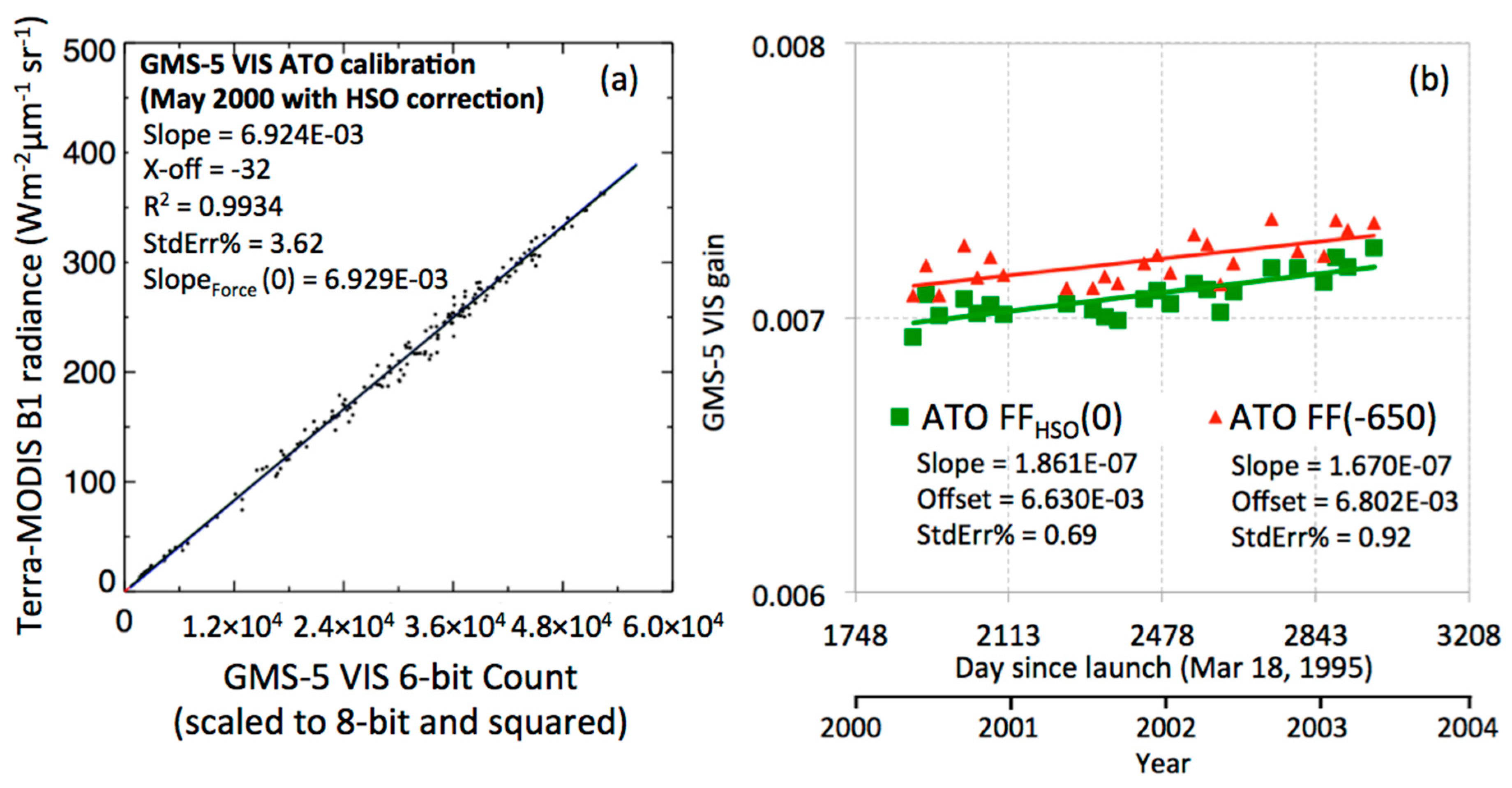
Figure 10.
GMS-5 calibration curves to convert 6-bit count to radiance based on the ATO-RM method using FF(−650) (green) and the FFHSO(0) (black). The difference between the two calibrations was a function of the count and is shown by the red curve.
Figure 10.
GMS-5 calibration curves to convert 6-bit count to radiance based on the ATO-RM method using FF(−650) (green) and the FFHSO(0) (black). The difference between the two calibrations was a function of the count and is shown by the red curve.
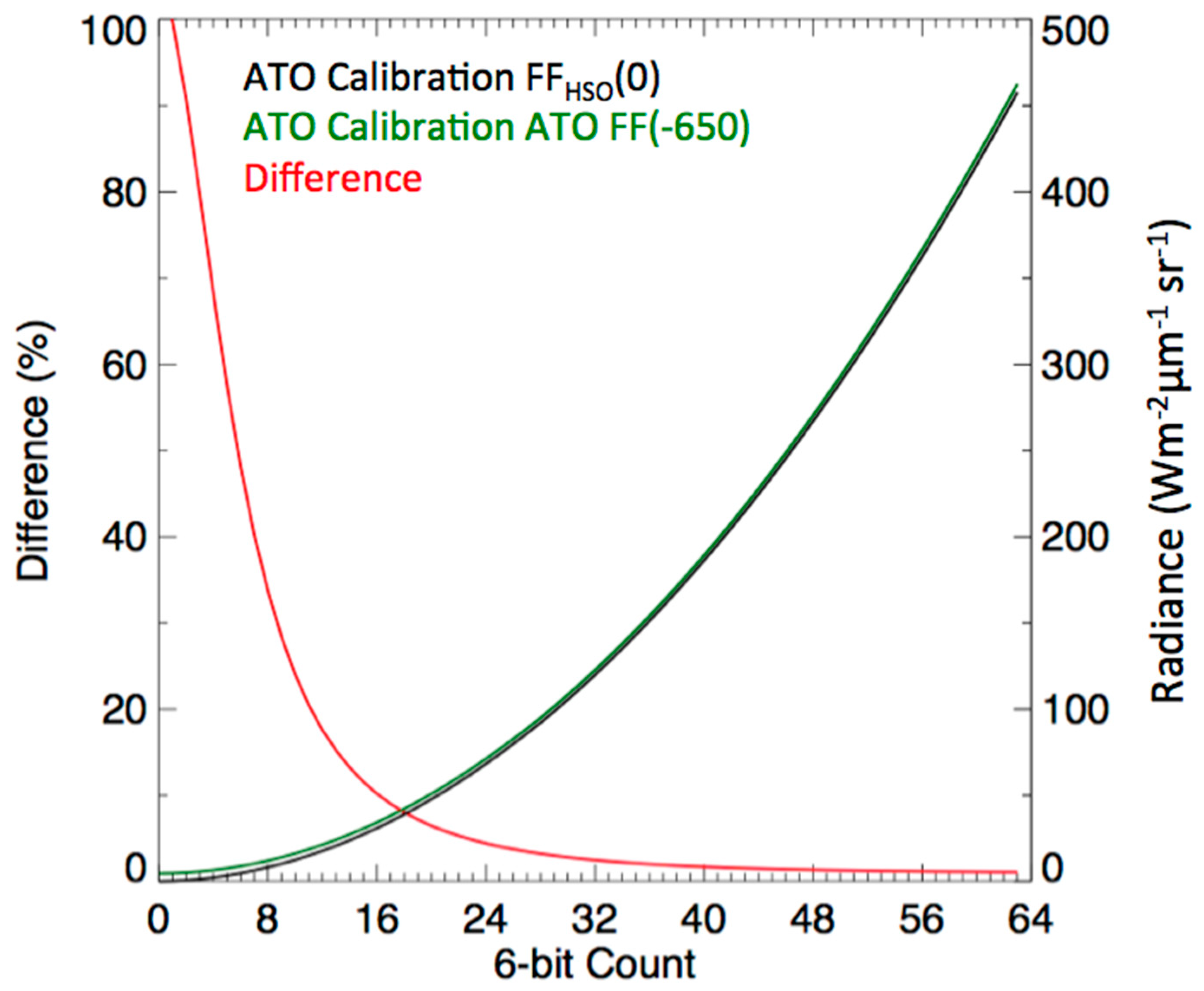
Figure 11.
(a) Comparison of monthly DCC mode radiance values from GMS-5 (red and black squares) and MTSAT-2 (blue squares). Red squares represent GMS-5 FF(−650) DCC mode radiances, whereas the black squares were computed using the FFHSO(0)-based calibration gains. (b) Similar to (a) except the comparison was made using the daily TOA reflectances computed over the Badain Jaran Desert.

© 2018 by the authors. Licensee MDPI, Basel, Switzerland. This article is an open access article distributed under the terms and conditions of the Creative Commons Attribution (CC BY) license (http://creativecommons.org/licenses/by/4.0/).
Share and Cite
MDPI and ACS Style
Bhatt, R.; Doelling, D.; Haney, C.; Scarino, B.; Gopalan, A. Consideration of Radiometric Quantization Error in Satellite Sensor Cross-Calibration. Remote Sens. 2018, 10, 1131. https://doi.org/10.3390/rs10071131
AMA Style
Bhatt R, Doelling D, Haney C, Scarino B, Gopalan A. Consideration of Radiometric Quantization Error in Satellite Sensor Cross-Calibration. Remote Sensing. 2018; 10(7):1131. https://doi.org/10.3390/rs10071131
Chicago/Turabian StyleBhatt, Rajendra, David Doelling, Conor Haney, Benjamin Scarino, and Arun Gopalan. 2018. "Consideration of Radiometric Quantization Error in Satellite Sensor Cross-Calibration" Remote Sensing 10, no. 7: 1131. https://doi.org/10.3390/rs10071131
Note that from the first issue of 2016, this journal uses article numbers instead of page numbers. See further details here.