Abstract
The automatic identification system (AIS) was developed to support the safety of marine traffic. In ice-covered seas, the ship speeds extracted from AIS data vary with ice conditions that are simultaneously reflected by features in synthetic aperture radar (SAR) images. In this study, the speed variation was related to the SAR features and the results were applied to generate a chart of expected speeds from the SAR image. The study was done in the Gulf of Bothnia in March 2013 for ships with ice class IA Super that are able to navigate without icebreaker assistance. The speeds were normalized to dimensionless units ranging from 0 to 10 for each ship. As the matching between AIS and SAR was complicated by ice drift during the time gap (from hours to two days), we calculated a set of local statistical SAR features over several scales. Random forest tree regression was used to estimate the speed. The accuracy was quantified by mean squared error and by the fraction of estimates close to the actual speeds. These depended strongly on the route and the day. The error varied from 0.4 to 2.7 for daily routes. Sixty-five percent of the estimates deviated by less than one speed unit and 82% by less than 1.5 speed units from the AIS speeds. The estimated daily mean speeds were close to the observations. The largest speed decreases were provided by the estimator in a dampened form or not at all. This improved when the ice chart thickness was included as a predictor.
1. Introduction
Ships navigating in ice-covered sea areas need ice information to support their operations. In the Baltic Sea, operative ice information includes daily ice charts, ice model forecasts, and ice thickness charts provided by the national ice services, in our case by the Finnish Ice Service (FIS). The production of the information relies strongly on synthetic aperture radar (SAR) imagery, both Sentinel-1 and Radarsat-2 imagery, typically obtained once or twice a day from each sea area. Experts of the Ice Service prepare the daily ice chart using the chart of the preceding day and other satellite images, in addition to using observations from icebreakers and coastal stations. The charts divide the ice cover into regions characterized by a set of parameters that comprises the concentration; typical, maximum and minimum thicknesses of level ice types; and a five-degree numeral for the degree of ice ridging (DIR). On the other hand, the level ice thickness chart is a supporting operative SAR-based product [1]. The product refines the level ice thickness information of the ice charts using SAR-based segmentation. The product has been operative for several years. It is validated annually using ship reports and more extensively in reference [2].
The difficulty of ice navigation is mainly due to ice ridges. Additionally, when assisted by an icebreaker, the ships must be able to proceed through the thick ice channel rubble that remains from the ridges broken by the icebreaker. The traffic restrictions to Northern Baltic ports are set in terms of the Finnish–Swedish ice classes where class IA ships may navigate to all ports throughout the winter season. Ships in the more powerful subclass IA Super are capable of independent navigation unless the conditions are exceptionally difficult. This may be due to very difficult ridging conditions, brash barriers or ice compression. A brash barrier (windrow) is a band of ice rubble at the ice margin that is typically 2 nautical miles wide and 10 m thick. It is created when thin ice is broken by waves and then compressed by wind against thicker ice. During compression, the ice cover is in a prevailing stress state that may manifest as channel closing, added resistance or even pileup of ice against the ship hull.
During normal conditions, ridge fields complicate the navigation system, especially the icebreaker assistance, by inducing performance variations between ships of different capabilities as well as speed variation for each individual ship. This includes occasional besetting, which, in convoy operations, increases collision risks and causes delays and disorder in port logistics. Better information about the distribution of ridged ice would improve the predictability of arrival times and make the winter navigation system generally more efficient and economical. For this reason, the detection and quantification of ridging from SAR imagery has been investigated from different aspects since the late 1980s. For Baltic Sea studies, see, for example, references [3,4,5,6,7,8].
On the surface, ridge rubble is usually arranged into narrow, elongated sails. The usual surface parameters to describe ridging are the sail height and ridge density, which is the number of ridge sails along a linear transect (e.g., a linear ship track). These surface parameters can be linked to the statistics of the subsurface ridge keels, which can, in turn, be used to estimate ship speed reduction. The ridge sail height and density are related to the horizontal coverage of the fraction of the surface area covered by ridge rubble [9], a parameter which contributes to the magnitude of in SAR images. Consequently, a connection exists between the backscattering intensity and the difficulty of navigation. Field campaigns carried out in the Baltic Sea ice have shown that variation in the C-band is mainly due to large-scale surface roughness (e.g., ridge rubble) [5,10,11,12]. Based on the SAR studies, it has been observed that, on average, the C-band increases when the intensity of ridging increases. Some figures can be found in [11,12]. The relationship is not unambiguous, as small-scale roughness, salinity and the incidence angle also contribute to the backscattering coefficient (e.g., new thin ice types can produce strong backscattering) [13].
Thus, results that are sufficiently reliable for operational implementation are still lacking, and attempts to derive the ridge height or surface rubble volume per unit area have been inconclusive [14], although the coverage of individual sails increases with the sail height. The same surface rubble coverage can result from shallow sails and a high ridge density or from high sails and a low ridge density. If the resolution of SAR imagery is too coarse (like 500 m) to allow ridge sails to be visible, the ridging parameters can barely be obtained from the aggregated contribution of ridges to in the pixel area. Recently, learning methods, such as the random forest classification of feature statistics [8], have shown promise in the determination of DIR from SAR images.
Another line in the utilization of SAR in winter navigation has been to provide the imagery to ships navigating in polar ice-covered seas [15,16,17]. Ships can use the images as an aid in route selection and tactical navigation by identifying leads, areas of low concentration or areas with low degree of ice ridging. The ice conditions ahead can be anticipated from SAR based on what has been experienced in the near past when navigating through ice fields with similar SAR texture. This can be supported by state-of-the-art SAR classifications and other ice information products supplied by the land base. The main problems are a limited communication bandwidth and the fact that in the presence of ice drift, it can be impossible to pinpoint the ship’s location in reference to the image, even when the image is only a few hours old.
Finnish and Swedish icebreakers in the Baltic Sea provide a working example of SAR-based operation planning. The SAR images used to prepare ice charts are also received by a geographic information system–type terminal software on icebreaker bridges and presented with other selectable layers of navigational and environmental information [16].
As the icebreakers may operate for weeks or months in the same sea area, the crew learns to link the SAR texture with degrees of navigational difficulty. This is facilitated by the fact that a large part of the SAR texture remains largely unchanged between two images, and the ice drift patterns are not too complicated in the semi-enclosed Baltic basins. However, this personal understanding is not easily expressed quantitatively or communicated to others (e.g., to the FIS). The two-way communication between the FIS and the icebreakers was discussed in [18].
The idea that a ship’s observed response to an image texture and features is used to interpret the image is inherent in all SAR-assisted navigation. We seek to develop this idea into a consistent methodology of SAR classification that can also be used to complement other methods to extract navigationally-relevant information from the images. The ship response is extracted from the AIS (automatic identification system), which is a messaging system for broadcasting navigational information from a ship to other ships and to onshore authorities. Among other things, the AIS messages report the location and speed of the ships. Since the AIS system became mandatory in 2002, the data has been used extensively to study maritime traffic and its impacts.
AIS data are particularly applicable in the Baltic Sea, with its intense and steadily growing ship traffic. There are approximately 2000 ships for which the AIS is mandatory at sea at any given moment heading to or from its 200 commercial ports. The annual amount of cargo is about 1 billion tonnes, and the ferries carry approximately 100 million passengers. The main research applications have been general spatiotemporal characterization and statistical analyses of the traffic systems in some sea areas [19] and the quantification of ship encounters and associated collision risks (e.g., [20]).
The cargo and passenger flow continue without interruption throughout the ice season, when, on average, half of the Baltic area becomes covered with ice. Icebreakers are also used to keep the ports open in the northernmost parts of the sea. The presence of ice modifies both the traffic patterns and risks, but also introduces traffic system features that are not present in open water conditions—especially icebreaker assistance and speed reduction and besetting due to ice conditions. AIS data have been used to assess the winter navigation system [16], navigation risks [21], icebreakers and convoy operations [22], ship ice performance [23,24], ice resistance modeling [25] and route selection [26].
We widen this domain of applications with a new approach where AIS data are used to interpret the SAR images in terms of attainable ship speed and locations of difficult navigation. As a first-order approach, the speed reductions observed at certain locations of the SAR image are taken to indicate that the location is navigationally difficult, and if several ships show a similar response, this is almost certainly so. As such, this would be valuable information along frequently-operated ice channels, and it is easily obtained if the ice is not drifting. However, we aim for a SAR-based classification of whole sea areas by studying the ship responses to SAR feature vectors constructed for this purpose. The methodology is based on random forest regression, the demonstration is conducted in ice-covered part of the Gulf of Bothia in March 2013, and the response is described in terms of the relative speed of independently navigating IA Super ships.
This paper is organized as follows. The data sets comprising AIS, SAR and ice chart data are described in Section 2. The random forest tree ensemble method to estimate ship speeds using SAR features and sea ice parameters extracted from the manual ice charts is presented in Section 3. Section 4 presents the results and the quantitative analyses of their accuracy, and the concluding Section 5 and Section 6 discuss the results and the future potential of the approach.
2. Data Sets and Processing
2.1. Ice Conditions during the Ice Season and Study Period
The time period of our study was March 2013, and the area studied was the Baltic Sea northward from the latitude of N. This covers the entire Bay of Bothnia and largely, the Sea of Bothnia, and the areal extent is about 92,000 . In the Bay of Bothnia, ice formation in the open sea started during the first week of December and the bay was fully ice-covered on 26 December. After a few days, winds decreased the coverage to 20% of the bay area. Full coverage was attained again on 17 January, after which the pack ice developed in phases of opening, ridging and refreezing. In the Sea of Bothnia, there was ice pack only close to the coast. At the end of February, the temperatures started to decrease and the extent of ice grew rapidly. The whole of March was extremely cold. The maximum ice extent covered 177,000 of the Baltic area of 422,000 , and was attained on 15 March. The extent was close to climatological average, but the date was later than usual. The Sea of Bothnia became fully ice-covered for the first time at the end of the month. In April, the ice retreated rapidly because the ice types formed in March did not have large thicknesses.
During the study period, the maximum average thicknesses of level ice types was greater than 50 cm in the Bay of Bothnia (see Figure 1 (upper panel)). Although the ice pack was mobile throughout the month, the winds were not particularly strong. The wind speeds fluctuated during the first week and settled at around 5 m/s with occasional spikes reaching 10 m/s. However, the wind direction varied greatly. In the Bay of Bothnia, this resulted in the opening of a lead and the formation of new thin ice alternatingly along the Finnish and Swedish coasts. This is shown in Figure 1 as lower monthly averages. The main pack of older and thicker ice suffered few changes, but rather, was shuffled back and forth. In the Sea of Bothnia, the ice cover started to expand more rapidly after the first week of March, and during the last ten days, southward ice drift accelerated the freezing of remaining open water areas. Ice ridging conditions were not difficult. The highest degree of ice ridging (i.e., Ridged 3 in Figure 1 (lower panel)) was atypically not present even in the Bay of Bothnia, and the Sea of Bothnia became only slightly ridged due to the moderate winds.
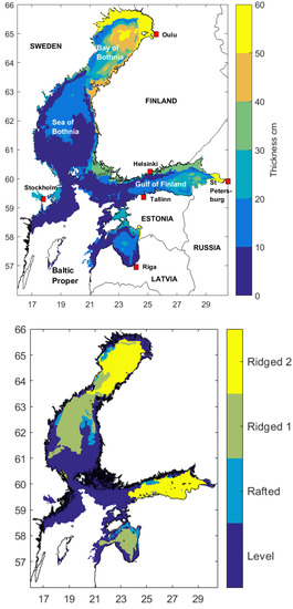
Figure 1.
Mean ice thickness and maximum degree of ridging in March 2013 (upper panel, lower panel). The maps are based on daily ice charts.
2.2. AIS Data
The AIS is a very high frequency system used for broadcasting information on ship state, and it has been mandatory for vessels over 300 gross tonnage and for all passenger vessels since 2002. The Finnish Traffic Administration (FTA) receives Baltic AIS data on terrestrial stations, conducts a quality check and redirects the data to the vessel traffic service (VTS) centers and other civil end users. The AIS data consist of different types of messages, many of which are optional. However, the basic navigational data are automatically coded in position reports (Type 1–3 messages) which include the ship identifier, location, speed, heading and course.
This AIS data stream has been received at the Finnish Meteorological Institute since 2007, arranged into a database and used for research purposes. The database links the position reports with marine environmental data and ship particulars data and provides search utilities that can be conditioned by time, geographic area, environmental parameters and ship particulars. The Type 1–3 message interval for a steaming ship is about 10 s, and the number of position reports for years 2007–2016 amounts to 6 billion. The main use of the database has been winter navigation research, in which the environmental data consists of gridded ice charts and ice model forecasts.
The main shortcoming of the AIS data is that the changes in propulsion power are not known. When studying a ship’s response to ice conditions, there is no guarantee that the observed speed reduction is due to the increased difficulty of ice conditions and not due to a change in the power setting. The power setting may be reduced when a safe encounter with other ships requires a slower speed, increased if the ice conditions ahead pose a besetting risk or changed either way in order to adjust to convoy speed. To minimize this uncertainty, we selected the group of independently navigating ships of the Finnish–Swedish ice class IA Super. The criterion of independency was that there were no ships within 3 nautical miles and none expected to come within 3 miles during the following 10 min. On the other hand, IA Super ships are able to navigate without icebreaker assistance unless the ice conditions are exceptionally difficult. They also usually do not change their power setting much when navigating independently [23].
The range of FTA terrestrial stations is limited. The coverage of the data decreases when moving close to the Western coastline of the Sea of Bothnia. For the Bay of Bothnia, the coverage is complete and the AIS message intensity (Figure 2) is measured by the number of position reports from square nautical miles per day for the IA Super ship class. The concentration of traffic to the main ice channels in the Bay of Bothnia is discernible. Outside these routes, the ships visited almost all locations within the pack ice except for an area in the middle of Bay of Bothnia where the ice was very thick (Figure 1). In the fast ice zone, the traffic is constrained to narrow channels leading to ports. The average traffic speed is the monthly average of speed records from a square nautical miles for the ship class IA Super. It is a summarizing descriptor that also includes ships that have been idling. It was observed that the traffic speed generally increased with a decreasing intensity in the Bay of Bothnia. This is due to powerful ships selecting routes outside the main ice channels occupied by the convoys of weaker ships led by icebreakers.
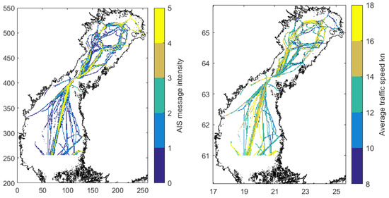
Figure 2.
Intensity of automatic identification system (AIS messages) and average measured speeds of IA Super ships in March 2013 (left, right).
In total, 21 IA Super cargo ships operated in March 2013 in our test area north of latitude 61 N. There were sister ships, and the number of ships with different particulars was 13. They comprised 700,000 position reports of independent navigation, and made up a total of 55 voyages. The size ranged from 4000 to 28,000 gross tonnage, and the length of vessels ranged from 105 to 215 m. We imposed a threshold speed of 1 knot to eliminate data of idling ships drifting in the ice. From the voyages, we further selected continuous test routes that constituted the basic data for our analysis. If a voyage took place on more than one calendar day, the track covered during each different day was regarded as a different route. The data for the ships contained gaps whenever the independency condition did not hold any longer, and less frequently if the AIS messages were not received from the Western part of the Sea of Bothnia. To eliminate short AIS records, it was required that only such transects for which at least 2000 AIS measurements were recorded consecutively during one day were included in the analysis. Finally, there were 139 routes in the data set, with a total length of 38,500 km. The fraction of the data used in the training of the regression model was about 23%, and the rest of the data was used in the testing. The training data were created by randomly selecting 30 routes from the AIS data set.
The ships generally had different icebreaking capabilities and ice transit speeds. It is possible to establish comparability by considering their speed relative to their maximum speed, which is often also their open water speed. Thus, in the analysis, we normalized the speed for each ship to a dimensionless unit of 0–10, where 10 indicates a high speed for each particular vessel. Speeds over 20 knots were considered to be outliers, and their normalised speed was set was set to 10 units. Hence, the formula from knots to units was
where v is the speed of an individual ship in knots and is the maximum speed recorded for the ship during March. We call the unit of the normalized speed simply “unit”. Approximately 2% of all AIS speeds in the training were set to 10 units. After the normalization, the relatively few recorded extreme speeds over 20 knots did not affect the estimation process as outliers.
2.3. RADARSAT-2 SAR Imagery
The SAR imagery used in this study was RADARSAT-2 ScanSAR Wide (RS-2 SCWA) dual-polarized imagery with the HH/HV polarization combination. The nominal size of an RS-2 SCWA image was approximately 500 × 500 km, and the pixel size was 50 m. The spatial resolution was approximately 73–163 m × 100 m (range by azimuth). The incidence angle () varied from to . The equivalent number of looks (ENL) was larger than six. The noise equivalent, , at both HH- and HV-polarizations was around −28 ± 2.5 dB, and the absolute accuracy of was better than 1 dB [27].
The preprocessing of the RS-2 SCWA images consisted of the calibration of and according to information included in the SAR images, georectification with Geospatial Data Abstraction Library (GDAL) software and calculation of the incidence angle, . The incidence angle correction and land masking was performed using in-house-developed software. First, the data were rectified into the Mercator projection with a pixel size of 100 m and a reference latitude of N. This georectification is compatible with the FIS ice charts and the navigation systems of the Finnish and Swedish icebreakers. During HV-polarization, the SAR values are close to the instrument noise floor (around −28 dB for RS-2 SCWA mode), and the noise floor (noise equivalent ) varies along the across-track direction. The calculation of the incidence angle correction was described in detail in reference [28] for the HH channel and in reference [29] for the HV channel.
A SAR mosaic covering the whole Baltic Sea was formed each day by employing enough processed RS-2 SAR images that there were no holes in the coverage of sea areas. The Baltic Sea SAR images were used to update the SAR mosaic twice daily. The number of images used to update the SAR mosaic over the study area varied from 0 to 1 SAR images per day. On average, the study area was partly covered by one new SAR image each day. For a specific location in the study area the SAR imagery was 0–2 days old, depending on the last acquisition time. The daily information from the acquisition of SAR data during the test period is shown in Table 2 in Section 4.6. Due to the large size of the SAR images in the SAR mosaics, the resolution was downsampled to 500 m.
2.4. Ice Charts
In our analysis, we also used the daily manual ice charts provided by the FIS over the Baltic Sea. The ice charting software divides the ice cover into polygons described by quantitative parameters and qualitative characterizations. The polygons and their quantitative parameters in ice charts were also saved as numerical latitude–longitude grids using the ice charting software. The usual grid resolution was degree of latitude and degree of longitude, which is approximately 1 nautical mile in both directions at N. Parameters in the grid format included the typical, minimum and maximum thicknesses of the ice level, ice concentration and the degree of ice ridging. These grids were converted to the Mercator projection used in the rectification of the SAR imagery. When combining the ice chart grids with the SAR mosaic, the nearest neighbor interpolation was used to find the chart value for the SAR pixels.
The information in the FIS ice charts was typically reported for rather large areas (hundreds of square kilometers). The level ice thickness values are based on the observations made by the operating icebreakers. According to the annual surveys where in-situ level ice thicknesses and typical level ice thicknesses by manual ice charts were compared, the mean difference was less than 10 cm (private communication by Alexandru Gegiuc). In the graphic FIS charts, the thickness values are given as a variation range between the minimum and maximum thicknesses. The gridded charts also include the typical thickness, which is the mean of the range. This value is also rounded to the nearest 5 cm if the result is at least 15 cm. We chose to use the mean value without rounding in order to have a denser gradation of thickness. The sea-ice concentration at FIS is based mainly on the SAR imagery, and—if the conditions allow—also optical data. This variable has an uncertainty of approximately 10% according to the ice experts at FIS.
3. Methodology for the Estimation of Ship Speed
A regression model to estimate ship speed from SAR images was constructed. The three principal steps in this process are described in this section: defining the SAR features for the regression model, training the model to estimate speed and evaluating the usefulness and relative importance of the features.
3.1. Features
To each SAR pixel, we attached a feature vector consisting of features that were expected to be relevant for the speed estimation. The SAR features were defined in terms of in some window centered at the pixel. As features external to the SAR image, we included ice thickness and ice concentration from the ice charts. The ship speed was the response variable in the regression, and to every AIS speed was assigned the feature vector pertaining to the pixel where the ship was located.
There was an unavoidable time gap of varying length between the SAR acquisition and the AIS messages. How accurately the ice conditions around the ship correspond to the SAR features at the same location depends on the magnitude of ice drift during the time gap. In the Baltic Sea, if the wind increases an ice concentration that already exceeds 70%, the ice cover is usually static unless the wind speeds exceed 10–15 m/s. If the concentration is lower, or the wind decreases its concentration, the onset of ice drift may occur at any wind speed. As a general rule, the ice drift speed after drift onset is 1–2% of the wind speed, and speeds exceeding 50 cm/s may be observed [30]. Thus, the ice may drift as much as 2 km per hour, although 100–300 m per hour is typical.
The backtracking of SAR information can be attempted by ice drift models or through the analysis of the SAR time series itself. It is mostly applicable at scales of tens of kilometers long (e.g., [31]). Drift is also partly compensated by the fact that the ice surface can remain statistically rather similar over relatively large areas. Hence, for the present study, we adopted an approach where the statistics were calculated in sliding windows of four different sizes: pixels (3.5 km scale), pixels (2.5 km scale), pixels (1.5 km scale) and the pixel itself (0.5 km scale) The features attached to the window or the pixel itself were in both polarizations. For the other windows, we selected the basic statistical measures of —the mean, the standard deviation (std), the maximum and the minimum, which were all calculated in both polarizations. In the feature vector level, we also included the ice thickness and ice concentration from the ice charts. This has the advantage of allowing us to discriminate between open water and ice cover without a separate classification phase.
We also tested the usefulness of some textural features. In our earlier studies, we observed that spatial autocorrelation ([32,33]) and entropy ([8,34,35]) are effective in SAR classification. Here, we computed them in a window size at a scale of 5.5 km in both polarizations. We also tested the coefficient of variation at scales of 3.5 km and 2.5 km in both polarizations.
Thus, the initial feature vector had, in total, 30 different SAR feature candidates: , two basic statistics (mean, std) for three window sizes, two statistics (maximum and minimum) for one window size, two textural features in one window size, and a coefficient of variation in two window sizes, for both polarizations. To these were added the ice thickness and concentration. In the final analysis, we reduced the size of the feature vector to 16 components. This is described after the regression model is presented in Section 3.2.
3.2. Random Forest Regression Model
As indicated earlier, the time gap between the AIS messages and the SAR data acquisition made estimation difficult. Our first attempt was to fit a feedforward neural network to the data to make predictions (e.g., [36]). This approach gave ship speed v estimates where the mean speeds along an individual route were close to the measured one. The weakness of the method was that the values of v were concentrated within a very narrow range—the high ship speeds (>8 units) were missing, as were the low speeds (<6 units).
We noted that the random forest regression (RFR) [37] yielded a larger spread for the estimated speed values, v. Hence, it was selected. Random forest is an ensemble learning method which can be applied to classifications and regressions. It is currently a rather popular method in data analysis (e.g., [8,38,39,40]). In RFR, several artificial training sets are generated from the original training set using bootstrapping, and then a regression tree is grown for each individual training set. Regression is performed for each tree, and finally, the results are aggregated. This is called bagging or bootstrap aggregation [37,41]. For the analysis, our data were divided into training and test data sets (see Section 2.2).
To gain an intuitive understanding of how a regression tree is grown, the basic principles underlying these trees are briefly discussed. The feature space is a p-dimensional rectangle, X. Using recursive binary partition, the regression tree divides X into M disjoint rectangles , which are represented by the terminal nodes of the tree. In each p-dimensional rectangle, , the response is modeled as a constant, . The training data consists of N observations with a p-dimensional feature vector, , and a response, . That is, the regression is performed using pairs, , where , with . We denote the tree’s prediction at input vector, x, with . The residual sum of squares (RSS) was adopted as the criterion function in the automatic splitting of a node in a regression tree and also in the selection of the splitting variable. The minimization of implies that the best estimate of in Equation (2) is the average of all in region —that is, [41]. The regression tree is
Hence, the structure of the regression function is a step function. The parameter characterizes the tree, T, in terms of split variables, split points at each node and terminal node values.
3.3. Random Forest Regression Algorithm
One of the advantages of RFR is that the feature vector can consist of many kinds of variables (e.g., continuous, discrete or categorical). An example of a categorical variable is the level ice thickness, which had six possible categories in our data set. In the previous section, the structure of a single regression tree was explained. Here, the algorithm is outlined to calculate the regression tree ensemble. A bootstrap sample from training set Z is denoted by . The bootstrap sample, , is of the same size as the original sample, so, on average, 63% of the original samples of Z belong to it, the rest being duplicates [42]. The samples of Z left out from (∼37% of the samples) are called out-of-bag samples.
B bootstrapped training sets, , are generated, and relying on every training set, a regression tree is grown . Hence, an ensemble of trees with is obtained, where for every tree a regression estimate is computed, as in Equation (2). The regression estimate of depends on the feature vector x which is used as input for the tree. This is denoted by . A regression tree often achieves a rather low bias if it is grown deep with many nodes without pruning [41]. On the other hand, a single tree has large variance.
In the regression, we recorded all the regression estimates provided by the ensemble of B trees for a specific feature vector (i.e., B regression estimates were acquired). If these regression estimates are averaged, then the ensemble estimate has a smaller uncertainty than a single regression tree, because an average has a smaller variance than a single variable. This is also true for the correlated variables. The problem with the presented bagging approach is that the grown trees are correlated. To reduce this correlation, RFR has a randomization step [37]. When building a tree, each time a split in a tree is considered, a random sample of m predictors is chosen as split candidates from the full set of p predictors. A new sample of m predictors is taken at each split. This step prevents the same features from dominating the ensemble. The flow of the random forest algorithm is presented below.
| Random forest algorithm for regression |
|
| Regression estimate for a new feature vector, : |
| Let be the ensemble of all of the regression trees constructed as described in the steps i to . Then, the random forest predictor is |
In the presented algorithm, the average of all regression estimates is taken. It is also possible to use other statistics. In fact, in the estimation we applied the quantiles computed from the set of regression estimates.
We ran all of our random forest regressions with the same set of tuning parameters using the routine TreeBagger [43]. From the set of sixteen () features, we randomly chose features to be used in a single split. The number of feature components and the value of m were selected on the basis of our pilot runs. If B is large enough, then the random forest algorithm avoids the tendency of overfitting the model, which often occurs in the context of decision trees. In our analysis, we used trees. We did not observe any notable improvement in the results when the number of trees was greater.
3.4. Importance of the Features
The selection of the final feature vector was based on both the accuracy of the estimation and the relative importance of the features. The out-of-bag samples were used to evaluate the features with respect to their relative importance. All out-of-bag feature vectors, about vectors per tree, were run through each tree of the ensemble. The following method was used to quantify the importance of a feature. For a single tree, all splits involving the feature were considered. The quantification was in terms of the change of the residual sum of squares before and after each split. The results were finally accumulated over the ensemble of all trees.
We note that none of the tested textural features were included in the Table 1. Note also that the standard deviations (std) of the values in all scales were excluded due to their negligible importance and negative impact on the estimation. Hence, the 14 final SAR features consisted of the very basic statistics: the mean, standard deviation, maximum and minimum.

Table 1.
The selected features presented in decreasing order of importance.
We remark that the importance of a feature depends on the other features selected to the feature vector in Table 1. We performed an experimental regression run using only the ten most important features. However, the estimation results were more erroneous than the ones obtained using all 16 components presented in Table 1. Note that the scales of 2.5 km and 3.5 km yielded the best results. This is a reasonable result, because the AIS locations with respect to SAR feature locations had uncertainty. We also observed that the maximum and minimum values in the HH-channel in the 2.5 km scale were highly important.
4. Results
4.1. Estimation Accuracy
The main statistic used to measure the estimation accuracy was the mean squared error (MSE):
where we denote the response variable by , its estimate by and the sample size by n.
The mean absolute percentage error (MAPE), also known as the mean absolute percentage deviation (MAPD), is a measure of the prediction accuracy that is used often in forecasting. It usually expresses accuracy as a percentage and is defined by the formula
where the symbols are the same as in Equation (4). The interesting feature of MAPE is that it gives a large weight to a situation where is small and the prediction is essentially greater. These kinds of situations are of particular interest to us because they identify the harshest ice conditions for a ship.
4.2. Estimation Accuracy in General
Figure 3 shows the distributions of the estimated and AIS speeds for the whole data set. The mean speeds of the distributions were almost equal: 7.57 units for AIS speeds and 7.55 units for estimates. Of significance is that the estimated values were concentrated in a narrower range than the AIS speed values. Approximately 6% of the AIS speeds were below 5 units, while this was true for only 1% of the estimates. Estimates below 3.5 units did not appear at all. In the upper tail of the distribution, 16% of the estimates and 27% of the AIS speeds exceeded 8.5 units. No estimated speed value was above 9 units, but 11% of the AIS speeds were. This limited range of the estimates compared to the actual speeds is a typical limitation of this kind of model.
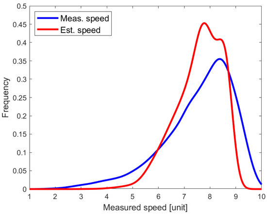
Figure 3.
The AIS (blue line) and estimated (red line) speed distributions.
In Figure 4, the assessment of the estimation accuracy is based on pointwise (pixelwise) differences between individual AIS speeds and their estimates. We note that in the 0.5 km pixel scale, 65% of all estimates were within 1 unit, 75% were within 1.25 units, and 82% were within 1.5 units from the correct value (colored blue in Figure 4). If we label all the errors with the absolute deviation value over 2 units in the 0.5 km scale as severe, then the amount of severe errors was 9%.
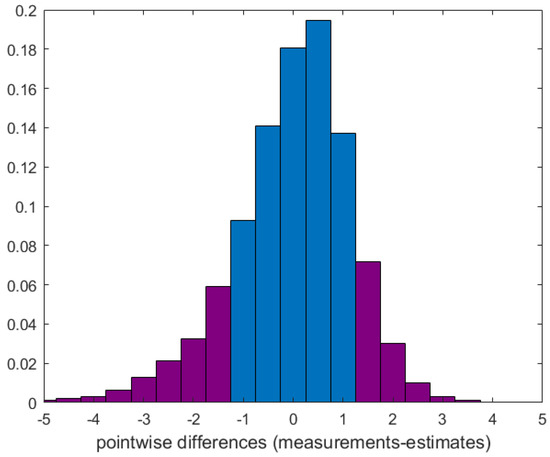
Figure 4.
The pointwise differences in the 0.5 km scale between AIS speeds and estimates for the whole test data set.
On average, the mean of the random forest regression slightly underestimated the routewise mean speeds. We corrected this by first calculating the quantile regression estimates for quantiles 0.2 and 0.85 and then taking the mean of those two speed estimates. This improved the accuracy of the results and was used in all reported results. This also includes the results shown in Figure 3 and Figure 4.
4.3. Estimation Accuracy in Different Ice Categories
In Figure 5 and Figure 6, we show the estimated and measured daily mean speeds plotted around the identity line. The parallel green lines deviate from the central line by one unit. The quantile regression can also be used to create an approximative confidence band for the estimates. However, this property was not utilized because the width of the estimated confidence band did not clearly indicate whether or not the prediction was close to the measured value.
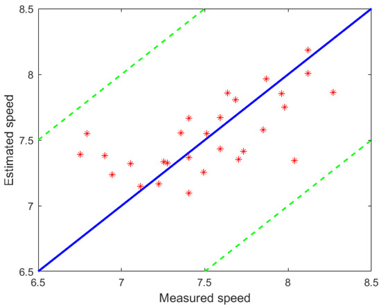
Figure 5.
The AIS and estimated mean speeds for the daily routes. The blue line is the identity line. The parallel green lines deviate from the central line by one unit.
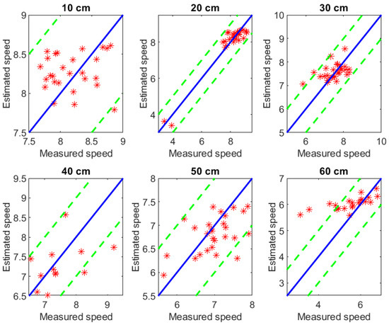
Figure 6.
The AIS and estimated mean speeds for each ice class. The blue line is the identity line. The parallel green lines deviate from the central line by one unit.
We also note that the mean speed error exceeded 0.5 units in only three out of 29 daily routes (see Figure 5 or Table 2). The maximum mean speed error was units (i.e., the estimated speed was larger). When taking the average over all daily routes, the estimated mean speed was only 0.013 units higher than the AIS-based mean speed.
Table 2.
Estimation results in March. M = AIS speed, E = estimated speed, MSE = Equation (4), MAPE = Equation (5), KL-d. = Equation (6), Estimates* = percentage of the pixelwise estimates that deviate from the AIS speeds less than one unit. Symbols for the SAR update: 2 = totally updated SAR coverage, 1 = partly updated, 0 = no updates.
To obtain a better understanding of how the ice thickness affected the accuracy of the daily mean speeds, we generated similar scatter plots for the following ice thickness classes: cl10 (1–10 cm), cl20 (11–20 cm), cl30 (21–30 cm), cl40 (31–40 cm), cl50 (41–50 cm), and cl60 (51–60 cm). Figure 6 shows that for the cl10 and cl20 thin ice categories, almost all of the estimation results were within 1 unit of the measured means. In cl30, the mean measured speeds and estimates were quite close to each other, except for some cases of lower measured speeds when overestimation took place. In two of the cl40 cases, a high measured speed (>8 units) resulted in underestimation. As discussed earlier, our regression procedure could not reproduce the very low speeds which occurred in thicker ice classes. The measured mean speeds in cl50 were mostly below the mean speed of the whole data set (7.5 units), and all the measured mean speeds were less than 8 units in cl60. On the other hand, very small mean speeds (<5 units) in cl50 and cl60 resulted in overestimation.
If the ships use channels made by the icebreakers, their speed in thick ice can be rather high in comparison with the icebreaking mode. The presence of open channels made speed estimations less accurate in thick ice than in thin ice in the Bay of Bothnia, manifesting as underestimations in the cl50 and cl60 categories. In cl60, over half of the cases were such that RFR overestimated the mean speed. If the regression model underestimated the mean speed, the recorded speed was rather high (>6 units) considering the ice thickness. It is likely that the ships used the existing channels in these cases, although the exact information is lacking.
4.4. Estimation of Speed Variation
Much of the information of the ice conditions is contained within the speed variation. One index for the navigability of a certain route is the standard deviation of its speed. Hence, it is of interest to look at how well the variation was preserved in the estimated speeds along the route. The estimated speed variation was significantly smoother than the recorded speeds. Over all routes, the mean std of AIS speed variation was 1.31 units, but the mean std of the estimated speed was only 0.83 units over all routes (i.e., only 63% of the measured variation). The respective ranges for the standard deviations were from 0.86 units to 1.78 units for AIS speeds and from 0.52 units to 1.13 units for estimates.
Another measure for the preservation of the speed variation is how close the histograms of the AIS speeds and the estimates are to each other. We investigated their relationship using the Kullback–Leibler distance (KL-distance) which, for discrete distributions, P (AIS speeds), and Q (estimates) is defined as follows [44]:
Hence, the KL-distance is the average difference in log probability between the true (P) and estimated (Q) distributions (i.e., its value tells how much information is lost when Q is used instead of P. If we have a pair of estimated distributions, then the candidate that minimizes KL-distance will be closer to the true distribution [45]. The KL-distance is not symmetric (i.e., ). The daily KL-distance values can be found in Table 2.
Figure 7 (left panel) shows evidence of the fact that, on average, the estimation accuracy decreased when the standard deviation of AIS speeds increased. For this data set, the prediction uncertainty according to MAPE increased from 6% to 24%. There was no such clear connection between the KL-distance and MAPE, except for very large KL-distance values. The likely reason for the lack of the correspondence between the KL-distance and MAPE is that no spatial information is incorporated in the KL-distance value, unlike in the MAPE measure.
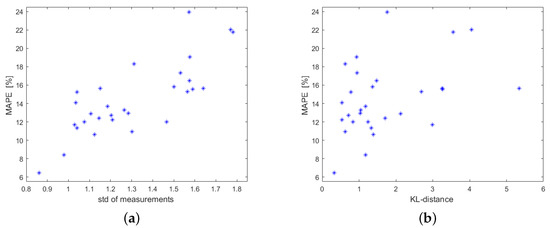
Figure 7.
The routewise std of the AIS speeds and MAPE (panel (a)). The KL-distance and MAPE (panel (b)).
4.5. Speed Charts
The major goal in this study was to create an estimated speed chart over the test area where every pixel value represents a typical speed for the specific ship class IA Super. We will now discuss two examples of such charts—one successful and one less successful.
In Figure 8 we present the results from March 8, 2013. The SAR imagery of the test area is in the upper-left panel and the histograms of the estimated speeds for the daily route and their AIS speeds are in the upper-right panel. The corresponding speed chart created by estimating every SAR pixel using the RFR method is in the lower-left panel, where the speed range is restricted from 5.5 to 10 units for sharper visualization. The daily route from 8 March, 2013 is overlaid on top of the chart with their AIS speeds in the lower-left panel. The speeds along the route are divided into three categories which are indicated by colors: red indicates AIS speeds from 8 to 10 units, purple indicates speeds from 6 to 8 units, and black indicates speeds less than 6 units. Upon the speed chart in the lower-right panel is marked how close the regression estimates were to the AIS speeds. If the difference is less than 1.5 units, the corresponding pixel is colored red. Otherwise it is marked black. We note that the MSE was 0.95 on 8 March 2013, which is considered a good result because the speed variation along the route was large (see Table 2). The AIS histogram in upper-left panel showed that the speeds were distributed rather evenly for a wide range, from 5.5 to 9.5 units. Additionally, lower AIS speeds were recorded. The estimated histogram also showed a wide spread with two peaks, at 6 units and at 8–8.5 units. The std of the estimated speed was close to the std of the AIS speeds, the values being 1.13 units and 1.47 units, respectively. The Kullback–Leibler distance describing the similarity of histogram had a value of 1.24.
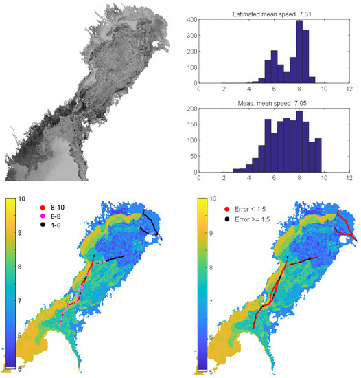
Figure 8.
Results from 8 March 2013. (Upper right): SAR image; (upper left) histograms (estimated and AIS speeds); (lower left) estimated speed chart and AIS speeds for the daily route; (lower right) estimated speed chart and estimation accuracy for the daily route. All speeds are in units.
In the panels of Figure 9, three different lines are drawn. The black line represents the level of ice thickness. It is scaled so that the actual thickness value in centimeters is divided by 10. Hence, a value of 2 refers to a thickness of 20 cm and likewise for the other values. The blue color represents the AIS speeds and red represents the estimates. The estimated and AIS speeds along the daily route of length 750 km in Figure 9 show that these two speed values were usually close to each other. Most of the differences occurred in rather thin ice areas (panels (c) and (d)) when the level ice thickness was either 10 cm (c) or 20 cm (d). Otherwise, the agreement was very good. For example, in panel (a), the speed estimates also exhibited variation in thin ice, as the AIS speeds did, due to the SAR statistics. The speed variation often increased when the ship moved from one ice regime to another. This can be seen clearly in Figure 9 and means that transitions from one ice category to another were often accompanied with a speed change. The most problematic areas from the point of view of estimation were thick ice areas (see Figure 6).
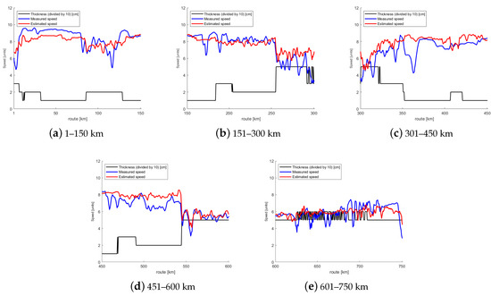
Figure 9.
The daily route recorded on 8 March 2013. Each panel (a–e) comprises a transect of 250 km. For an explanation of the used coloring, see the text.
Figure 10 shows a similar panel to Figure 8 with identical ordering, but for 20 March 2013. It illustrates a case where the estimation was less successful. The AIS speed variation was high with a large number of AIS speeds exceeding 9 units. Additionally, very low AIS speeds (less than 5 units) were recorded. The estimated speeds had a more limited range, from 6 to 9 units. The std of the AIS speeds was 1.78 units, and the std of the estimates was significantly lower, just 0.93 units. Hence the measured std was almost twice as large than the estimated std. The Kullback–Leibler distance had a very large value (KL–distance = 3.55), indicating a large discrepancy between the measured and estimated histograms. We see from Figure 10 that large estimation errors (black color) occurred both in thin and thick ice areas (lower-right panel).
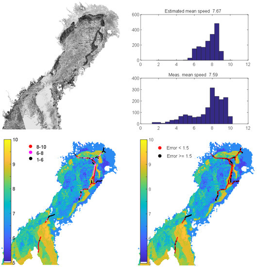
Figure 10.
Results from 20 March 2013. (Upper right) SAR image; (upper left) histograms (estimated and AIS speeds); (lower left) estimated speed chart and AIS speeds for the daily route; (lower right) estimated speed chart and estimation accuracy for the daily route. All speeds are in units.
The total length of the daily transects was again about 750 km (Figure 11). We will now inspect, in more detail, where the estimation failed. In transect (a), the agreement was relatively good in both thin and thick ice. In transect (b), both large and low ship speeds were recorded in thick ice (cl50). This initially led to an underestimation of ship speed in cl50 and later, an overestimation. The AIS recordings showed speeds close to 10 units in part of the cl50 transects (b,c). These panels are an example of the ambiguous nature of ship speed in thick ice. In the lower panels(d,e), the largest differences between the measured and estimated speeds took place in cl40 and cl30 (i.e., in thinner ice). The occurrence of short cl50 intervals in (d) did not have an effect on the ship speed but had some effect on the estimated ship speed. Instead, the somewhat thinner ice (cl40) slowed the ship speed, although this was not reflected in the estimated speed. The discrepancy between the AIS speeds and estimates continued in transect (e) in thin ice areas. Finally, we note that the average speeds taken over the daily data were quite close to each other: 7.59 for the AIS speeds and 7.67 for the estimates. Additionally the black segments (speed error over 1.5 units) are in the minority in the lower-right panel in Figure 10.
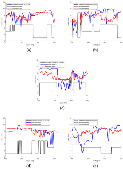
Figure 11.
The daily route recorded on 20 March 2013. Each panel (a–e) comprises a transect of 250 km. The coloring and lines are as described in Figure 9.
4.6. Collected Results
Table 2 presents several different daily statistics. We have already discussed the mean speed estimation and its accuracy. Here, those values are given for each day. Another measure of the estimation accuracy is how large a fraction of the speed estimates were close to the respective AIS speeds. We defined that the estimate was close to the AIS speed if their difference was less than 1 unit. The daily fluctuation of this fraction was large, ranging from 41% to 87%. The mean for the whole month was 64%. The spatial information is incorporated in this concept. If we consider estimates with an allowed deviation of 1.5 units from the correct value, the fraction of the included estimates varied from 63% to 96% per route, the average being 81%.
We also looked at how the presence/lack of fresh SAR data affected the estimation. In Table 2, the SAR updates are divided into three different categories, as follows: new SAR imagery over the study area was acquired (number 2), a small fraction of the study area in the northernmost part of the Bay of Bothnia was covered with fresh SAR imagery (number 1), no new SAR data was acquired over the study area (number 0). The impact of fresh SAR imagery varied (see Table 2) depending on the ice conditions. As noted in Section 2.1, in March, the winds were weak or moderate after the first week of the month (usually around 5 m/s with occasional spikes reaching 10 m/s). The acquisition time affected the estimation accuracy results somewhat (e.g., the mean KL-distance in the SAR acquisition category 2 was 1.4 and in categories 1 and 0, it was about 2.0).
5. Discussion
5.1. Uncertainties
Our approach was developed from the basic idea that ship speeds change with ce conditions in a consistent manner. The starting assumption was that average speed and speed variation correlate with the average ice thickness and thickness variation. However, there are missing pieces that make the implementation of this idea problematic when relying on AIS data alone. Firstly, without propulsion power it is not known for sure what speed changes are due to ice conditions. There are also engineering models that derive speeds for specific ship types from propulsion power, hull particulars, and ice conditions. These would provide a basis for predicting the ice performance of some ship types from the observed performance of another ship type. The lacking uniformity of icegoing capabilities of ships is the second missing piece in an approach relying solely on AIS data. The third is that most ships follow frequently navigated ice channels. For the channels, not only the ice resistance but also dynamic and thermal evolution are different from the surrounding intact ice cover.
We sought to minimize these problems by restricting the analysis to independently navigating IA Super ships. These are mostly able to make steady progress in Baltic Sea ice conditions and do not change their power setting much. For the IA Super class, the ice performance also varies much less between different ship types than is the case for lower ice classes. Finally, the IA Super ships often select routes outside the main channels in order to bypass convoys. On the other hand, although the progress in the channels is easier, they still display thickness variation in the surrounding ice cover; in particular, there are thick channel rubble sections remaining from broken ridges.
The uncertainties from channel navigation, a lack of propulsion power and different performance capabilities could be further reduced by also considering the variation in speed over short time scales corresponding to few ship lengths of transit. As such, variation is induced by the ridges. The speed should drop at the same locations for all ships. Adding the speed variation to the present approach could not only improve the results, but provide a method to quantify ice ridging from SAR images.
The inclusion of lower ice classes generally greatly increases the amount of data. The present results intended to demonstrate the soundness of the approach using a limited dataset, scratching the surface of the data comprising billions of AIS position reports from ten years and covering a wide range of ice conditions. Apart from increasing the amount of data, there are several possible future lines of research that are addressed in the next section.
5.2. Future Prospects of the Approach
To the best knowledge of the authors, this is the first attempt to generate ice navigation information from the direct classification of SAR imagery with ship data. Similar methods have great application potential. Approaches seeking to generate navigationally relevant information by linking SAR signatures with ship performance can be divided into three types: data-driven, classification-oriented and hybrid. In the Baltic Sea, more than 60 million position reports from ice-going ships are obtained every month, and it is perfectly feasible to generate maps of navigational difficulty from this data alone. A primitive approach would simply identify the SAR locations where several ships have difficulty. This cumulating information could be transferred to the next image for the part that has remained similar. In the first instance, this could be done by the charting experts of the Finnish Ice Service, as a similar task is already a daily routine for standard ice chart variables. This is helped by the fact that most traffic is constrained to ice channels which are rather easily identified. Channels also make the problem essentially one-dimensional, as along-track conditions are sufficient. Although navigation outside the main channels is common (see Figure 2), providing SAR-based navigability indices for them would be very useful for ships.
On the other hand, our approach is oriented towards SAR classification. Such methods seek to extrapolate the information gained from ship responses to certain SAR features to the whole image area. The extrapolated parameter can be speed (as in the present case), some numeral for navigational difficulty, or the load level experienced by the ship. There are also options for partial but more reliable extrapolation. The areas with difficult ice conditions are often discernible band-like formations created by previous stormy periods. The difficulty experienced when transsecting the band is likely to be close to the truth when extrapolated to the whole band. This is especially true for brash barriers (windrows) which usually have homogeneous properties in the along-band direction.
The present approach also has application potential in ice routing, where the objective is to optimize the route with respect to travel time or fuel consumption. The bottleneck has been that ice information has lacked the necessary detail for the calculation of ship speed from ice conditions. Our approach, in fact, indirectly demonstrates that routing is feasible in the Baltic Sea. Approximately one-quarter of the AIS speeds in our data set were used for training, and the rest were used for validation. In a similar manner, the ship data collected during the first quarter of some time period could be used to generate a speed map used in routing during the remaining period. The data from the routed ships could, in turn, be used to update the speed maps for the ships arriving later. The applied regression method works better the more comprehensive its training data set is. Therefore, such an incremental increase of the training data set should constantly improve the estimates.
In a hybrid approach, the AIS-based SAR classification is combined with other classification methods, especially those seeking to retrieve ice thickness, ice concentration and ridging parameters. Our approach applied the thickness and concentration from ice charts, but it could also have used parameters from SAR-based products that are used in FIS ice charting [1]. A promising direction of research is integrating AIS-based SAR classification with methods seeking to retrieve ridging for SAR. In reference [8], we introduced a method to retrieve the degree of ice ridging used in ice charts. Thus, one evident step would be to add the degree of ice ridging as one categorical variable to the current regression model. Further developments could also utilize ice forecast models and kinematic algorithms for ice drift. Additionally, engineering models describing how ship performance depends on ice conditions could be used to theoretically connect the AIS-based SAR methods with the existing methods of ice parameter retrieval from SAR.
6. Conclusions
We presented an approach that uses position and speed data from the AIS messages of ice-going ships to translate SAR images over ice cover to ship speed maps. The methods were demonstrated for Baltic Sea SAR mosaics for March 2013, for a ship class with good ice performance. When developed further, the approach has the potential to address various needs of the ice navigation community. This includes improved ice information and route optimization. It also has relevance for maritime engineering research seeking to model ship ice performance. The method relies on the random forest regression. The applicability of this advanced and recently much-used method was demonstrated in the present context. It was able to generate useful speed maps from a limited training set, although there are several uncertainties involved in the use of AIS data. Several possible lines of future research have been recognised.
7. Data Availability
All Matlab programs to analyze the data can be obtained by contacting the first author. The access to the AIS data is restricted. It requires acceptance by the Finnish Traffic Administration. The SAR data can be delivered only for research purposes and requires approval by FMI.
Author Contributions
Formal analysis, M.S. and M.L.; Funding acquisition, M.L.; Investigation, M.S. and M.L.; Methodology, M.S.; Software, M.S.; Writing—original draft, M.S. and M.L.; Writing—review & editing, M.S. and M.L.
Funding
Markku Similä and Mikko Lensu were supported by the BONUS STORMWINDS project funded jointly by the EU and the Academy of Finland (contract 291683).
Acknowledgments
We thank Alexandru Gegiuc and Juha Karvonen for the processing of the SAR mosaics and making valuable comments.
Conflicts of Interest
The authors declare no conflict of interest.
References
- Karvonen, J.; Similä, M.; Heiler, I. Ice Thickness Estimation Using SAR Data and Ice Thickness History. In Proceedings of the 2003 IEEE International Geoscience and Remote Sensing Symposium, Toulouse, France, 21–25 July 2003. [Google Scholar]
- Karvonen, J.; Similä, M.; Haapala, J.; Haas, C.; Mäkynen, M. Comparison of SAR Data and Operational Sea Ice Products to EM Ice Thickness Measurements in the Baltic Sea. In Proceedings of the 2004 IEEE International Geoscience and Remote Sensing Symposium, Anchorage, AK, USA, 20–24 September 2004. [Google Scholar]
- Johansson, R.; Askne, J. Modelling of radar backscattering from low-salinity ice with ice ridges. Int. J. Remote Sens. 1987, 8, 1667–1677. [Google Scholar] [CrossRef]
- Similä, M.; Leppäranta, M.; Granberg, H.B.; Lewis, J.E. The relation between SAR imagery and regional sea ice ridging characteristics from BEPERS-88. Int. J. Remote Sens. 1992, 13, 2415–2432. [Google Scholar] [CrossRef]
- Calström, A.; Ulander, L.M.H. Validation of backscatter models for level and deformed sea ice in ERS-1 SAR images. Int. J. Remote Sens. 1995, 16, 3245–3266. [Google Scholar] [CrossRef]
- Manninen, A. Surface morphology and backscattering of ice-ridge sails in the Baltic Sea. J. Glaciol. 1996, 42, 141–156. [Google Scholar] [CrossRef]
- Dierking, W.; Dall, J. Sea-Ice Deformation State From Synthetic Aperture Radar Imagery—Part I: Comparison of C- and L-Band and Different Polarization. IEEE Trans. Geosci. Remote Sens. 2006, 54, 3610–3622. [Google Scholar] [CrossRef]
- Gegiuc, A.; Similä, M.; Karvonen, J.; Lensu, M.; Mäkynen, M.; Vainio, J. Estimation of degree of sea ice ridging based on dual-polarized C-band SAR data. Cryosphere 2018, 12, 343–364. [Google Scholar] [CrossRef]
- Lensu, M. The Evolution of Ridged Ice Fields. Ph.D. Thesis, Ship Laboratory Report Series M-280, Helsinki University of Technology, Helsinki, Finland, 2003; 140p. [Google Scholar]
- Dierking, W.; Pettersson, M.I.; Askne, J. Multifrequency scatterometer measurements of Baltic Sea ice during EMAC-95. Int. J. Remote Sens. 1999, 20, 349–372. [Google Scholar] [CrossRef]
- Mäkynen, M.; Hallikainen, M. Investigation of C- and X-band backscattering signatures of the Baltic Sea ice. Int. J. Remote Sens. 2004, 25, 2061–2086. [Google Scholar] [CrossRef]
- Similä, M.; Mäkynen, M.; Heiler, I. Comparison between C band synthetic aperture radar and 3-D laser scanner statistics for the Baltic Sea ice. J. Geophys. Res. Oceans 2010, 115, C10056. [Google Scholar] [CrossRef]
- Lundhaug, M. ERS SAR studies of sea ice signatures in the Pechora Sea and Kara Sea region. Can. J. Remote Sens. 2002, 28, 114–127. [Google Scholar] [CrossRef]
- Dierking, W.; Lang, O.; Busche, T. Sea ice local surface topography from single-pass satellite InSAR measurements: A feasibility study. Cryosphere 2017, 11, 1967–1985. [Google Scholar] [CrossRef]
- Johannessen, O.M.; Alexandrov, V.Y.; Frolov, I.Y.; Sandven, S.; Pettersson, L.H.; Bobylev, L.P.; Kloster, K.; Smirnov, V.G.; Mironov, Y.U.; Babich, N.G. Application of SAR for ice navigation in the Northern Sea Route. In Remote Sensing of Sea Ice in the Northern Sea Route: Studies and Applications; Springer: Heidelberg/Berlin, Germany, 2007; pp. 323–396. [Google Scholar]
- Kotovirta, V.; Jalonen, R.; Axell, L.; Riska, K.; Berglund, R. A system for route optimization in ice-covered waters. Cold Reg. Sci. Technol. 2009, 55, 52–62. [Google Scholar] [CrossRef]
- Hui, F.; Zhao, T.; Li, X.; Shokr, M.; Heil, P.; Zhao, J.; Zhang, L.; Cheng, X. Satellite-Based Sea Ice Navigation for Prydz Bay, East Antarctica. Remote Sens. 2017, 9, 518. [Google Scholar] [CrossRef]
- Eriksson, P.B.; Majaniemi, S.; Lensu, M.; Karvonen, J. Met-Ocean Services by FMI for Ice Management and Shipping in Ice. In Proceedings of the OTC Offshore Technology Conference, Houston, TX, USA, 5–8 May 2014. [Google Scholar]
- Arguedas, V.F.; Pallotta, G.; Vespe, M. Maritime Traffic Networks: From Historical Positioning Data to Unsupervised Maritime Traffic Monitoring. IEEE Trans. Intell. Transp. Syst. 2018, 19, 722–732. [Google Scholar] [CrossRef]
- Zhang, W.; Goerlandt, F.; Montewka, J.; Kujala, P. A method for detecting possible near miss ship collisions from AIS data. Ocean Eng. 2015, 107, 60–69. [Google Scholar] [CrossRef]
- Goerlandt, F.; Goite, H.; Banda, O.A.V.; Höglund, A.; Ahonen-Rainio, P.; Lensu, M. An analysis of wintertime navigational accidents in the Northern Baltic Sea. Saf. Sci. 2017, 92, 66–84. [Google Scholar] [CrossRef]
- Goerlandt, F.; Montewka, J.; Zhang, W.; Kujala, P. An analysis of ship escort and convoy operations in ice conditions. Saf. Sci. 2017, 95, 198–209. [Google Scholar] [CrossRef]
- Lensu, M. Assessing the ice performance of ships in terms of AIS data. In Proceedings of the International Conference on Port and Ocean Engineering under Arctic Conditions, Trondheim, Norway, 14–16 June 2015. [Google Scholar]
- Montewka, J.; Goerlandt, F.; Kujala, P.; Lensu, M. Towards probabilistic models for the prediction of a ship performance in dynamic ice. Cold Reg. Sci. Technol. 2015, 112, 14–28. [Google Scholar] [CrossRef]
- Kuuliala, L.; Kujala, P.; Suominen, M.; Montewka, J. Estimating operability of ships in ridged ice fields. Cold Reg. Sci. Technol. 2017, 135, 51–61. [Google Scholar] [CrossRef]
- Montewka, J.; Goerlandt, F.; Lensu, M.; Kuuliala, L.; Guinness, R. Toward a hybrid model of ship performance in ice suitable for route planning purpose. SAGE J. 2018. [Google Scholar] [CrossRef]
- MDA (MacDonald, Dettwiler and Associates, Ltd.). Radarsat-2 Product Description; MacDonald, Dettwiler and Associates, Ltd.: Richmond, VA, USA, 2014; p. 84. [Google Scholar]
- Mäkynen, M.; Manninen, A.; Similä, M.; Karvonen, J.; Hallikainen, M. Incidence Angle dependence of the statistical properties of the C-Band HH-polarization backscattering signatures of the Baltic sea ice. IEEE Trans. Geosci. Remote Sens. 2002, 40, 2593–2605. [Google Scholar] [CrossRef]
- Karvonen, J. Evaluation of the operational SAR based Baltic Sea ice concentration products. Adv. Space Res. 2015, 56, 119–132. [Google Scholar] [CrossRef]
- Leppäranta, M. The Drift of Sea Ice, 2nd ed.; Springer: Heidelberg/Berlin, Germany, 2011. [Google Scholar]
- Williams, J.; Tremblay, B.; Newton, R.; Allard, R. Dynamic preconditioning of the minimum September sea-ice extent. J. Clim. 2016, 29, 5879–5891. [Google Scholar] [CrossRef]
- Similä, M. SAR image segmentation by a two-scale contextual classifier. SPIE 1994, 2315, 434–444. [Google Scholar]
- Karvonen, J.; Similä, M.; Mäkynen, M. Open Water Detection from Baltic Sea Ice Radarsat-1 SAR Imagery. IEEE Geosci. Remote Sens. 2005, 2, 275–279. [Google Scholar] [CrossRef]
- Cover, T.M.; Thomas, J.A. Elements of Information Theory, 2nd ed.; John Wiley & Sons: Hoboken, NJ, USA, 2006. [Google Scholar]
- Karvonen, J.; Shi, L.; Cheng, B.; Similä, M.; Mäkynen, M.; Vihma, T. Bohai Sea Ice Parameter Estimation Based on Thermodynamic Ice Model and Earth Observation Data. Remote Sens. 2017, 9, 234. [Google Scholar] [CrossRef]
- Bishop, C.M. Pattern Recognition and Machine Learning; Springer: Heidelberg/Berlin, Germany, 2006. [Google Scholar]
- Breiman, L. Random forests. Mach. Learn. 2001, 45, 5–32. [Google Scholar] [CrossRef]
- Zhang, H.; Li, Q.; Liu, J.; Shang, J.; Du, X. Image Classification Using RapidEye Data: Integration of Spectral and Textual Features in a Random Forest Classifier. IEEE J. Sel. Top. Appl. Earth Observ. Remote Sens. 2017, 10, 5334–5349. [Google Scholar] [CrossRef]
- Ruescas, A.B.; Hieronymi, M.; Mateo-Garcia, G.; Koponen, S.; Kallio, K.; Camps-Valls, G. Machine Learning Regression Approaches for Colored Dissolved Organic Matter (CDOM) Retrieval with S2-MSI and S3-OLCI Simulated Data. Remote Sens. 2018, 10, 786. [Google Scholar] [CrossRef]
- Hu, S.; Liu, H.; Zhao, W.; Shi, T.; Hu, Z.; Li, Q.; Wu, G. Comparison of Machine Learning Techniques in Inferring Phytoplankton Size Classes. Remote Sens. 2018, 10, 191. [Google Scholar] [CrossRef]
- Hastie, T.; Tibshirani, R.; Friedman, J. The Elements of Statistical Learning, 2nd ed.; Springer: Heidelberg/Berlin, Germany, 2011. [Google Scholar]
- Efron, B.; Tibshirani, R.J. An Introduction to the Bootstrap; Chapman & Hall/CRC Monographs on Statistics & Applied Probability; CRC Press: Boca Raton, FL, USA, 1993. [Google Scholar]
- MATLAB and Statistics Toolbox Release; The MathWorks, Inc.: Natick, MA, USA, 2016.
- Kullback, S. Information Theory and Statistics; John Wiley & Sons: New York, NY, USA, 1959. [Google Scholar]
- McElreath, R. Statistical Rethinking: A Bayesian Course with Examples in R and Stan; Chapman and Hall/CRC Press: Boca Raton, FL, USA, 2016. [Google Scholar]
© 2018 by the authors. Licensee MDPI, Basel, Switzerland. This article is an open access article distributed under the terms and conditions of the Creative Commons Attribution (CC BY) license (http://creativecommons.org/licenses/by/4.0/).