Growth of Retrogressive Thaw Slumps in the Noatak Valley, Alaska, 2010–2016, Measured by Airborne Photogrammetry


1
National Park Service, Arctic Inventory and Monitoring Network, Fairbanks, AK 99709, USA
2
Fairbanks Fodar, Fairbanks, AK, USA
*
Author to whom correspondence should be addressed.
Remote Sens. 2018, 10(7), 983; https://doi.org/10.3390/rs10070983
Submission received: 2 May 2018
/
Revised: 24 May 2018
/
Accepted: 8 June 2018
/
Published: 21 June 2018
(This article belongs to the Special Issue Remote Sensing of Dynamic Permafrost Regions)
Abstract
:We monitored the growth of 22 retrogressive thaw slumps (RTS), dramatic erosion features associated with thaw of permafrost, in the Noatak Valley of northern Alaska using high-resolution structure-from-motion digital photogrammetry. We created time-series of 3–6 Digital Elevation Models (DEMs) and orthophoto mosaics during the time period from 2010–2016 at each slump, using high-resolution digital single-lens reflex (SLR) photographs taken from airplanes or helicopters. DEMs created using airborne GPS camera locations were adequate to detect elevations changes as small as 10 to 15 cm. Measurements made on these DEMs and orthophotographs showed slump growth rates of up to 38 m yr−1, with the fastest rates on slumps with scarps of moderate height (1 to 4 m) exposing Pleistocene glacial ice. Most of the slumps grew at constant or declining rates during the study, apparently as a result of the slumps encountering more gentle topography as they expanded upslope. Sedimentation was predominantly on the slump floor within 40 m of the active scarp, and the zone of accumulation migrated upslope with the scarp, away from adjacent water bodies. This study demonstrates that low-cost cameras coupled with airborne GPS and no ground control are suitable for monitoring geomorphic change on the order of decimeters and are a powerful tool for monitoring in remote settings.
1. Introduction
Among the most dramatic erosion features associated with permafrost thaw in northern Alaska are retrogressive thaw slumps [1] (RTS; Figure 1). Retrogressive thaw slumps occur where an escarpment retreats by thaw of ice-rich permafrost [2]. Ice-rich material of substantial thickness (e.g., a meter or more) and lateral extent is needed to produce an RTS [3]. The escarpment typically migrates up a gentle slope; material falls or slides onto the adjacent slump floor, and then is transported further downslope by flow or water erosion. RTSs often occur near rivers, lakes, or the ocean and can shed large amounts of sediment into the adjacent water body [4,5]. Disturbance of the vegetation and organic surface soil layers by slumping results in increased soil temperatures, soil pH, and shrub productivity [6,7]. Warming temperatures of recent decades in the arctic have been linked to increased activity of RTS [3,8,9,10,11].
Numerous RTS have been identified in the National Parks of northern Alaska [12,13]. The National Park Service (NPS) has selected a set of relatively large and high-impact RTS for intensive monitoring by detailed three-dimensional (3D) modeling and analysis of changes over time [14,15,16]. This monitoring is a part of the long-term permafrost monitoring program of the NPS the Arctic Inventory and Monitoring Network (ARCN) [17,18].
Structure-from-motion (SfM) digital photogrammetry has been used with great success in topographic studies in recent years [19,20,21,22]. The vast majority of SfM studies to date have relied on ground control points to scale and georeference the digital elevation models (DEMs) and orthophotographs obtained from SfM processing. In our remote study area, ground control can only be obtained with expensive helicopter landings, leading us to seek an alternative method, based on airborne GPS, that was developed over the course of this study.
We monitored the 3D form of 22 RTS by creating time-series of photogrammetric digital elevation models (DEMs) and orthophotomosaics. Our time-series starts with high resolution satellite images (IKONOS) taken in 2008. Our earliest DEMs were made in 2010 by taking hand-held oblique photographs from a helicopter or fixed-wing aircraft with no onboard GPS, by the first author. The resulting SfM models were scaled by helicopter landings and placement of aerial targets and total station survey of the targets, in one year, and other years were registered to the resulting model using natural landmarks [14,15,16]. Beginning in 2013, we began using fixed-wing aircraft with a vertically mounted camera coupled to a survey-grade GPS with precise timing, operated by the second author, at first through the University of Alaska Fairbanks and then commercially starting in 2016 [23,24]. The development of software that could georeference a 3D model from camera GPS locations alone made it possible to forego helicopter landings, making our operations less expensive and less time-consuming. We used natural landmarks visible on our pre-2013 oblique photographs and the 2013–2016 georeferenced models to register DEMs and orthophotos from the earlier oblique photos. These oblique photo-derived DEMs were less accurate but still useful for extending our time series.
While previous studies have investigated the distribution and growth of RTS in relation to environmental factors [3,8,9,10,25,26,27,28,29,30,31], our methods provide greater spatial and temporal resolution in 3D than previous studies. Here we use this unique data set to increase our understanding of the growth rates and factors that influence them in the RTS of the Noatak Valley of northern Alaska.
In this report we refer to the steep, migrating face of an RTS as the “main scarp,” in keeping with the geological literature on landslides and mass movements [32], rather than the “headwall,” a glaciological term with another meaning that has become widespread in the RTS literature.
2. Materials and Methods
2.1. Study Area
We monitored the growth of 22 retrogressive thaw slumps located in the Noatak River basin of northern Alaska (Figure 2; slump coordinates are given in the Supplementary Online Materials Table S1). This is a region of continuous permafrost [33] and arctic tundra vegetation of cotton sedge (Eriophorum), sedges (Carex), and various low to mid-sized shrubs (Betula, Salix, Vaccinium, and Dryas sp.) [34].
The study area was glaciated during the late Pleistocene, and the study slumps are mostly in glacial deposits from the Itkillik I and Itkillik II glaciations [35]. The Itkillik II glaciation coincided with the last worldwide glacial maximum (marine isotope stage II). The Itkillik I glaciations are older than the Itkillik II but occurred after the previous interglacial [35,36]. Relict glacial ice from these advances has been observed in escarpments of retrogressive thaw slumps [13,14].
The mean annual, mean July, and mean January temperatures at the nearest long-term weather station, the Noatak Remote Automated Weather Station (RAWS; Figure 2) for the period of record (1990–2016) were −7.0, +12.8, and −23.7 °C, respectively [37]. The thaw season (daily means above 0 °C) typically runs from mid-May through mid-September. The annual total thaw degree-days (TDD; degree-days with base temperature of 0 °C) at Noatak RAWS averaged 1237 degree-days for 2008–2016 (the time interval for most of our data). Trends in TDDs over the period of record (Figure S1) were weak; linear regression and a Mann-Kendall test for monotonic trend for the period 1990–2016 both show positive slopes but non-significant p-values of 0.37 and 0.43, respectively. Trends in TDDs for the period of most of our slump monitoring (2008–2016) were clearly non-significant, with p-values of 0.99 and 1.00 for linear regression and the Mann-Kendall test. Permafrost temperatures in the study area are mostly −4 to −7 °C, based on modeling by Panda et al. [38] (Table S2). Active-layer thicknesses under undisturbed vegetation in the study area are currently approximately 0.5 m (Table S2) [33,38,39].
Precipitation data are available from Noatak RAWS for the summer season; precipitation is important in slump growth processes [30]. For the period of record 1990–2016, precipitation data for June, July, and August were available for all years except 1991, 1999, 2003, and 2016. The mean June–August precipitation was 129 mm, and trends with time for the period of record were weak: a linear regression and Mann-Kendall trend tests have p-values of 0.79 and 0.77, respectively (Figure S2). For the time period of most of our slump observations (2008–2016), the weak upward trend suggested by inspection of Figure S2 is not supported by linear regression or Mann-Kendall test: p-values were 0.36 and 0.39, respectively.
2.2. Imagery and Analytical Methods
Most of our measurements were based on the analysis of DEMs and orthophotos that we created by SfM digital photogrammetry. Our main image sources were oblique aerial photos from 2010 to 2012 and vertical aerial photos from 2013 to 2016 (Table S1). The oblique photos were taken by D. Swanson from the window of a helicopter or fixed-wing aircraft with a Nikon D700 digital SLR camera and 50 mm lens, on multiple linear passes near the slump. All 22 study slumps have two or three years of these images. The scale of oblique photos varies greatly across any given frame, but the photo centers were generally 200 to 400 m from the camera, yielding a ground resolution at the center of 4 to 7 cm. In one of the years with helicopter access we landed at each of these slumps and marked 5 to 11 ground points in or near each RTS with temporary 1.5 m by 1.5 m square targets that we could identify on the photographs from that date. We then measured the targets’ relative positions using a Topcon GTS-235W total station. In one to three years during 2013–2016, M. Nolan took vertical aerial photographs from a fixed-wing aircraft of all of the study slumps except one (NOAT172) using a Nikon D800 digital SLR camera and 24 mm lens at 300 to 600 m above ground level, for an average ground resolution of 6 to 12 cm. Photo centers were located with accuracy of about 10 cm measured by on-board GPS [23]. These photos were taken along pre-determined flight lines to optimize overlap and the photogrammetric bundle adjustment within the processing software (Agisoft Photoscan [40]). The use of precise coordinates in the photo’s exterior orientation eliminated the need for ground control, a major cost and time savings for remote work like this, conducted hundreds of miles from the nearest logistical hubs. Prior studies using this technique [23,24] have found a geolocational accuracy of 30 cm and a repeatability of 10–20 cm; that is, two maps may have a misfit of up to 30 cm in any direction, but once this mean is removed the random and systematic noise is on the order of 10–20 cm at the 95% RMSE level, depending on acquisition details. This was the first application of modern (SfM) photogrammetry applied to the study of RTS using air control rather than ground control to produce maps that could resolve change at the decimeter to centimeter level.
The pre-2013 photos were georeferenced using the 2013–2016 models by selecting multiple points on landmarks around the slump perimeters on the 2013–2016 models; these points were then located on the earlier (unregistered) 3D models. We used these landmarks as pseudo-ground control points in the photogrammetric bundle adjustment in Photoscan to produced georeferenced models for 2010–2012. The final orthophotographs were resampled to 10 cm and DEMs to 20 cm in most cases. All of the slumps also had two-dimensional (2D) data from IKONOS satellite images (1-m pan sharpened resolution) from 2007 or 2008. Three of the slumps also had vertical digital photos from 2006 or 2008 taken by Tom George with a Nikon D2X camera and 24 mm lens. The slumps thus had data from 4–7 years, of which 3–6 years were 3D data.
We used the ground surveys from 2010 to 2011 as a check on the accuracy of the models created from the 2010–2012 oblique photos. We compared our measurements of distance and elevation change between the targets in the field to those same measurements derived from the DEMs and orthophotos.
For NOAT172, which lacked the aerial georeferencing in any year, and GAAR008, which had just a single flight pass of vertical photos and lower resolution (about 0.4 m), we georeferenced the year 2010 model using the ground survey points and registered other years to this model by landmarks as described above.
The time intervals between photography of any given slump varied: image dates ranged from 21 June through 25 September, and not all slumps were photographed every year. As a result, photos from consecutive years in some cases were separated by the better part of two thaw seasons (e.g., photos from July of year 1 and September of year 2). For this reason, simply dividing the change in slump area or scarp position by the number of calendar days or years separating these visits would be misleading. To correct for the irregular temporal spacing of samples and the fact that growth only occurred during the thaw season, we analyzed slump change in relation to accumulated thaw degree-days (TDDs). Slump growth rates are controlled by complex energy balance conditions at the slump scarp [41], but TDDs are a convenient integrator of the energy available for slump growth in the absence of detailed energy-balance measurements. We computed the change in slump area and linear change in position of the slump scarp per accumulated TDD using temperature data from the Noatak RAWS ([37] Figure 2). The resulting rates are in unfamiliar units of change in area or distance per TDD. Thus we converted them back to the more familiar units of area or distance per year using the mean value of 1237 TDD yr−1 for the Noatak RAWS (2008–2016). We used the mean value for TDD yr−1 because, as noted previously, the annual sum of TDD exhibited year-to-year variation but no consistent trend during the study time interval. Furthermore, because the time intervals between measurements were unique to each slump and incorporated portions of multiple thaw seasons, there was no straightforward way to define what the unique value for TDD yr−1 was for each interval between measurements.
As justification for normalizing growth rates using data from the Noatak RAWS, we note all of the slumps are within about 100 km of the Noatak RAWS and have annual average TDD sums (based on gridded monthly means from [42] similar to the Noatak RAWS (Table S2). In addition, our use of thaw degree-days to normalize the time between samples requires only that the annual pattern of TDD, not the absolute values, be similar between sites. For example, we observed 50.75 m of scarp retreat on slump NOAT069 between consecutive visits on 19 July 2011 and 10 September 2012. During this time interval, 1780 TDD accumulated at Noatak RAWS, which was 1780/1237 = 1.44 times the average annual total TDD. The 1780 TDD sum exceeded the average annual value not because of unusual weather, but because significant parts of two thaw seasons separated the sample dates. If we assume that the annual pattern of TDD at slump NOAT069 is similar to the Noatak RAWS, then 1.44 times the annual average TDD should have accumulated between 19 July 2011 and 10 September 2012 at slump NOAT069 also, and the normalized annual growth rate at NOAT069 would be 50.75 × 1237/1780 = 35.3 m yr−1.
The Noatak RAWS had missing temperature data for about 10% of the days in May–September (i.e., the thaw season) of 2000–2016. We filled missing temperature data at Noatak RAWS with predicted values from a linear regression between thaw season mean daily temperatures at Noatak RAWS and the next closest weather station with data for our period of observation, Kelly RAWS (Figure 2) [37]. Details of this process are in the Supplementary Materials and Tables S3 and S4.
We digitized slump perimeters by hand on the orthophotographs. In some cases the main scarp retreated by formation of long fissures parallel to the scarp, separated by elongate turf blocks [15]. Here, we defined the perimeter of the slump at the uppermost fissure. These features were not readily located by automated means, hence our choice to use manual digitizing. To compute the rates of scarp migration (in linear units per TDD), we manually digitized a baseline up the approximate centerline of the slump and measured linear distance along the centerline from the lower perimeter of the slump to the main scarp. We computed scarp heights along the centerlines at the intersections of the hand-digitized centerlines and slump perimeters as follows. The elevation along the centerline 1 m from the digitized scarp position on the undisturbed side of the scarp was taken as the top of the scarp. The foot of the scarp was found by locating the best fit of two lines to the elevations along the centerline below the scarp (Figure 3).
Our georeferenced orthophotographs from different years displayed sub-meter x-y agreement and were not adjusted further. DEMs from different years also generally showed sub-meter elevation agreement in areas expected to be unchanged (i.e., outside of the slumps). The agreement between DEMs from different dates was evaluated as follows. We created a buffer zone extending from 10 to 50 m outside of the digitized outer perimeter of the slump on the flanks and uphill side. This area was expected to have been unchanged between the two DEM dates. We computed zonal statistics (mean and standard deviation) for the difference between the two DEMs in this buffer zone
Because the slope of the slump below the scarp was constantly changing (due to deposition of material) and often irregular, we related slump growth to the original (undisturbed) slope along the centerline. The slope was computed by differencing the original (undisturbed) elevations between scarp positions from consecutive samples and dividing by the distance along the centerline between them. We used scarp elevations from the earliest topographic model (2010 in most cases), because this provided undisturbed elevations for the future scarp positions. To reconstruct the undisturbed elevation at the escarpments in 2008 (satellite data from prior to our first models), we interpolated the 2010 contour lines from outside the slump across the disturbed area where this appeared reasonable (i.e., where the slump was narrow and had matching contour lines on either side).We used a linear model [43] to study the relationship between slump growth rate per TDD and slope steepness at the active scarp.
We estimated the dates of inception of slumps from inspection of historical aerial photographs and satellite imagery. These consisted of c. 1955 panchromatic aerial photographs, the Alaska High-Altitude Photography (AHAP) color-infrared photographs from c. 1980, and Landsat images from the 1980s up to the present. We compared these to slump initiation dates for many of the slumps from synthetic aperture radar image analysis in the literature [13].
3. Results and Discussion
3.1. DEM Agreement
The differences between DEMs from two dates created using vertical photos with airborne GPS were very consistent in the buffer zones (10 to 50 m outside the slump perimeter): standard deviations for the difference between 2013 and 2016 DEMs ranged from 5.0 to 7.6 cm (Table 1). These results are comparable to previous results with our mapping system [23,24]. These low standard deviations allowed us to correct the difference DEMs by simply subtracting a constant correction factor, the mean difference between the DEMs for the buffer zone, which ranged from 0.254 to 0.487 m (Table 1). Since two standard deviations encompass over 95% of a normal distribution, we can say with better than 95% confidence that any difference between the two DEMs of more than 10 to 15 cm represents a true elevation difference. Note also that the scale of our topographic changes (meters) is an order of magnitude greater than the noise (decimeter). The photo texture was sufficient for image correlation and point cloud generation everywhere on our images except water bodies. DEM differences were noisier in areas of tall shrubs, where SfM point clouds represented both canopy and ground surface. Tall shrub vegetation was present only outside of slump perimeters and thus we did not attempt to filter out canopy points before DEM creation. Similar DEMs may be obtained using LIDAR [23,44], but at greater cost due to the much more complex technology involved. Satellite synthetic aperture radar (SAR) data is capable of centimeter-scale elevation measurements, but as yet cannot match the spatial resolution of low-altitude aerial photographs [45,46].
The DEMs created from 2010 to 2012 oblique photos, registered to the GPS-georeferenced DEMs from 2013 to 2016 vertical photos, displayed systematic variation in the elevation difference of up to a meter or more between two DEM dates in areas outside of the slump. In other words, the DEMs created from the 2010 to 2012 oblique photos showed tilting or warping relative to the DEMs from the 2013 to 2016 vertical photos and to one another. The resulting statistics for the 10–50 m buffer zone showed low mean differences between the DEMs (because the DEMs from the oblique photos were created using pseudo ground-control points from 2013 to 2016) but high standard deviations due to warping. For example, at slump NOAT148 the mean difference between the 2010 and 2013 DEMs was 0.046 m and the standard deviation was 0.870 m. The distortion of the models based on oblique photos is probably due to a variety of causes including (1) the highly variable scale of these photos (ranging from less than 10 cm in the near foreground to more than a meter in the distant background); (2) the minimal parallax between adjacent photos for more distant background objects, equivalent to a very low photogrammetric base-height ratio; (3) the difficulty for the software in recognizing common features from oblique photos on flight lines of different orientations, which forced us to use single flight passes in some models; and (4) the difficulty in finding precise natural features to use as tie points to the georeferenced models in our study landscape.
Because of this result, we limit our DEM difference analysis to comparisons among the 2013–2016 DEMs. However, comparison of the distances and elevations separating aerial targets on the models created from pre-2013 oblique photos with measurements obtained by total station survey indicate that the internal dimensions of these models are fairly accurate (Table S5). The individual distances between survey targets as measured on the models differed from those obtained by total station survey by maximum of 2.5% in the horizontal distance and 1.5% vertical (i.e., 1.5 m elevation error over 100 m of horizontal distance). However, the average error across all 80 test points was just −0.06% horizontally and +0.02 m vertically, which indicates good overall dimensional accuracy of the models (Table S5). Thus we were able to use the less accurate 2010–2012 models to digitize slump perimeters, and compute slopes and scarp heights.
3.2. Ground Ice and Geologic Setting
Exposures in slump main scarps were adequate to observe ground ice characteristics in 16 of the 22 slumps (Table 2). Ground ice in these exposures was of three main types. (1) Ten of the 16 slumps with good exposures lacked ice wedges but had a laterally continuous body of glacial ice under 1.5 to 2 m of glacial till (Figure 4). This overburden thickness greatly exceeds the typical active-layer thicknesses in the area under undisturbed vegetation (about 0.5 m). Glacial ice fit the criteria of Murton et al. [47]: laterally continuous, massive, aggregate-poor ice containing a range of suspended mineral particles from sand and silt to occasional pebbles and cobbles, and a sharp thaw or erosion upper contact with overlying poorly sorted sediment identified as glacial till. The majority of these slumps were in material mapped as glacial drift from the last glacial maximum (LGM), though four were in sediments mapped as older glacial drift or glaciolacustrine sediments (Table 2) [35]; (2) Five of the 16 slumps with good exposures had large, dark-colored ice wedges in glacial till or in loess over glacial till (Figure 5). These were the typical late Pleistocene ice wedges that are common in Alaska in frozen sediments that were exposed during the last glacial maximum (e.g., Kanevskiy et al. [48]). They suggest that the till is from a pre-LGM glacial advance. Of the five slumps with exposed ice wedges, we observed glacial ice under the till in four of the five slumps, and we do not discount the possibility that glacial ice was present but obscured in the remaining one. These spectacular exposures revealed ice wedges penetrating the loess and till and, in a few cases, the underlying glacial ice (Figure 5). Four of the five slumps with ice wedges were, as would be expected, in areas mapped as pre-LGM glacial drift [35] (Table 2). These drifts were exposed to ice-wedge accumulation during the LGM; (3) Finally, one slump (NOAT265) had a very high escarpment with sediments well exposed that lacked visible massive ice (Figure 6). This area was mapped as possible Quaternary terrace gravel [35], though observations of poorly sorted, weakly stratified material in the scarp suggest glacial drift. Though lacking visible massive ice, this material was obviously ice-rich, as shown by its liquefaction with thaw.
Relict Pleistocene glacial ice has been observed in thaw slump escarpments at multiple locations in the Noatak Valley [13,14]. The total area of Pleistocene glacial drift mapped in the Noatak Valley [35,49] is about 2900 km2. Ice-cored glacial terrain is particularly vulnerable to change as a result of permafrost thaw [11,50]. Permafrost temperatures in the upper Noatak Valley are expected to rise from their current levels of −4 to −7 °C up to 0 to −3 °C by the end of the current century (Table S2) [38]. Active layers are expected to increase during the same time interval to be near 1 m under undisturbed vegetation [38], which is less than the 1.5 to 2 m of till overburden that we observed in most slump scarps. Thus we expect that disturbance of the vegetation and organic surface soil, and/or removal of some of the overburden by other erosion processes, will still be required to trigger RTS in the upcoming decades. However, increasing permafrost temperatures and thickening active layers in the future are likely to greatly increase the amount of RTS activity triggered by such local disturbance.
3.3. Growth Rates and Environmental Factors
The scarp height and slump growth-rate characteristics were closely related to the slump ground ice characteristics. In an example year (Table 2), the scarp heights in slumps with exposed ice wedges (3.9 to 8.6 m) were generally taller than the slumps with glacial ice but no ice wedges (1.3 to 3.9 m). The anomalous slump NOAT265, with little exposed ice, had the highest scarp (12.2 m on the centerline). The fastest scarp retreat rates, up to 35 m yr−1 in the example year, were observed in the slumps with glacial ice and no ice wedges. The range of scarp retreat rates for the example year in the slumps with ice wedges (1 to 13 m yr−1) overlapped the lower half of the range for slumps with glacial ice only (1 to 35 m yr−1). The slumps with poor exposures had slumped material obscuring their escarpments and slow scarp migration rates (less than 2 m yr−1). The single most rapid centerline retreat rate was 38 m yr−1 by slump NOAT070 in 2010–2011.
Most of the study slumps grew throughout the study time period, with growth rates steady or declining over time as measured both on an area basis (Figure 7) and as the distance of scarp retreat along the centerline (Figure 8). Growth was closely related to the accumulated sum of TDD. Simple quadratic curves fit to area vs. accumulated TDD had regression r2 values of 0.98 or better in all cases (Table S6), while quadratic curves fit to scarp position along the centerline vs. accumulated TDD had regression r2 values of 0.97 or better (Table S7). The negative values of the coefficient a (the squared term in the equation) in all except one case in each of Tables S6 and S7 indicate a concave downward curve, i.e., a slowing growth rate per thaw-degree-day over time.
Slump growth studies with multiple observations within a single thaw season show slump growth rates to be slower early in the season that would be expected from energy balance measurements [41,45]. This is probably one source of the error between individual points and the fitted curves of slump growth vs. TDD in Figure 7 and Figure 8, and we would caution against assuming that slump growth at multiple points within a thaw season will correlate closely with TDD. The good fits between slump growth and TDD we observed support the utility of TDD as a way to normalize measurements taken at irregular intervals of a year or more.
A plot of scarp retreat rate along the centerline vs. topographic slope (of the undisturbed surface above the scarp) for all the study slumps and available time intervals (Figure 9) suggests that very fast scarp movement (e.g., more than 20 m yr−1) can occur only on slopes of 5% or more. The blank area in the upper left of Figure 9 probably represents the region where rate of retreat was limited by slope. However, inactive scarps (retreat rates near zero) also occurred on slopes up to 10% (Figure 9).
The topographic slopes of the undisturbed surface along the future slump centerline prior to slumping were concave downward in most cases (Table S8, Figure 10), i.e., the slope declined over time as the slumps grew uphill; this suggests that decreasing slope could explain the decreasing growth rates per TDD of the slumps over time. To test the hypothesis that declining slope was responsible for the declining rate of slump growth over time, we fit this linear model
where g is the growth rate of the slump in m per TDD between all consecutive pairs of samples, a and b are regression coefficients, i is the slump identifier, s is the topographic slope of the undisturbed surface, and “:” signifies the interaction of the slump identifier and the topographic slope, i.e., the slope-growth rate relationship was fit separately for each slump. This model was highly significant (p < 0.001) overall, but the relationship between slump growth rate and topographic slope was highly significant (p < 0.05) for just 9 of the 22 slumps. The remainder either had large error or were missing because the topographic slopes were near zero (NA in Table S9). All of the slumps with significant growth rate-topographic slope relationships showed the expected positive effect of slope on growth rate. The r-squared value indicates that topographic slope and slump together explain 68% of the variance in slump growth rate per TDD.
g = a + b(i:s)
The fastest linear growth rates were not associated with the tallest escarpments (the largest circles in Figure 9). As mentioned above, the tallest scarp was observed on slump NOAT265 (the two large, black circles on the right in Figure 9); this slump was on the steepest slope and had intermediate rates of scarp retreat. The slumps with ice wedges (green in Figure 9) had tall scarps, and slow to intermediate scarp retreat rates on a wide range of slopes.
Slump growth rates along the centerline were not closely related to the compass orientation of the scarp (Figure 11). The orientation of the scarp centerline changed little as the slumps grew, but a wide range of orientations were present in the different slumps in our data set. The fastest growth rates were observed on slumps that had west- or north-facing scarps (Figure 11). Slumps with maximum growth rates greater than 20 m yr−1 were observed on slopes facing all four cardinal directions (north 315–45°, east 45–135°, south 135–225°, and west 225–315°).
Intuition suggests that greater radiation due to direct sunlight on south-facing slumps should result in faster growth rates, and in one study in northwestern Canada slumps grew faster on south- and west-facing slopes [31]. However, energy balance measurements show that other terms in the energy budget, notably sensible and latent heat from the air, can dominate and allow the energy expenditure for ice ablation to greatly exceed net radiation [51]. Indeed, our maximum overall slump growth of 218 m over 7.8 thaw seasons (8 September 2008 to 7 November 2016, 9663 TDD), or about 28 m yr−1, was on the north-facing slump NOAT069; this shows what ablation can be accomplished with little direct solar radiation. Ice-cliffs on debris-covered glaciers (which are, in essence, escarpments of retrogressive thaw slumps) are more common, steeper, and less debris-covered on north-facing than other aspects, probably as a result of differences in the radiation balance between the upper and lower parts of the scarp [52,53]. Similar processes may allow our north-facing RTS to maintain growth rates as high or higher than south-facing RTS.
The rates of scarp retreat in this study are similar to those reported in other studies [6,9,25,27,29,31,54]. Correlations between rates of RTS scarp retreat and environmental factors in the literature are somewhat contradictory. Lacelle et al. [31] compared growth rates of RTS in northwestern Canada over 20 years as determined from Landsat images (30 m resolution) with topographic factors (from a DEM of similar resolution) and climatic factors, and found only scarp aspect had a significant correlation. Wang et al. [27,29] tracked growth rates of 18 RTS for three seasons in northwestern Canada with on-the-ground measurements and found a positive relationship with scarp height, but not aspect. Wang et al.’s plot of scarp retreat rates vs. slope was similar to ours: inactive slumps were present across a range of slopes; the fastest retreat rates were on moderate slopes (about 14%), with declining maximum growth rates on steeper and gentler slopes. Slopes of at least 7% were needed for growth of coastal RTS in northwestern Canada [55]. Our view is that the factors of topographic slope, scarp aspect (and related measures of solar radiation), summer warmth, and scarp height should all have some effect on slump growth rate, but that these effects can easily be overwhelmed by the unique effects of ground ice and sediment characteristics of each individual slump. Within the lifespan of a single slump, aspect varies little but slope at the scarp can vary as the scarp migrates. Thus, in the growth of a particular slump, the slope and ground ice conditions are likely to control the rate of growth.
3.4. Reconstructing Initiation Dates and Predicting Future Slump Growth
Disturbed, bare soil from the current episode of slump activity was first visible at many of the study slumps in the mid-2000s (Table 3). The initiation of these slumps probably resulted from the unusual weather of 2004, which had a very early and wet spring followed by a warm summer [13].
The slumps that started in the mid-2000s decade appear to have grown at rates since their inception that are roughly predictable from what we observed 2008–2016. If we extrapolate back in time the quadratic curves fit to the observed area growth, most of the curves for slumps that started in the mid-2000s intersect the x-axis (the point where the slump area was zero) within a few years of their observed initiation dates (Table 3). These extrapolations are most accurate for slumps where our data encompasses most of the growth, and not for slumps such as NOAT247 and NOAT248, which grew little since our monitoring began in 2008. Clearly, to understand the early growth of a new slump requires timely acquisition of imagery. The ability to mobilize quickly and target a specific area is an advantage of digital aerial photographs. Once located, slumps are long-lived features that can be readily resampled with digital aerial photographs.
The close fit of quadratic models to the slump growth rates vs. TDD (Figure 7 and Figure 8) suggests that the growth rate for an individual slump is predictable in the near future (e.g., the next one or two thaw seasons). As a test of our ability to predict growth in the near future from our data, we omitted the last observation, fit quadratic curves to the remaining 3 to 6 years of slump growth data, and used the fitted curve to predict the last observation. For the 22 slumps the mean percent error in predicting slump area at the last observation was −0.2% of the final area (standard deviation 7.2%); for linear growth along the centerline, the mean prediction error was 1.4% of the final length (standard deviation 5.8%).
3.5. Prior Slumping and Active-Layer Detachments
Fourteen of the 22 slumps occurred on ground undisturbed by previous slumping, based on interpretation of aerial photographs from about 1980, the Alaska High-Altitude Photography (AHAP) photo set (Table 3). In the other eight cases, the current slumps overlapped areas that had previously slumped, but all had expanded outside of previous slump boundaries to varying degrees. Five of these 8 slumps had visibly stabilized and revegetated prior to the re-activation in 2004–2005, and thus only three were clearly active prior to the 2004–2005 initiation event. Re-occurrence of RTS on the footprint of earlier slumps is common [3,8,10,26,56]. Repeated slumping shows that the prior pass by the main scarp of an RTS did not exhaust the supply of ground ice. Relict glacial ice provides particularly favorable conditions for repeated slumping, because many meters of nearly pure ice may be present. We observed about 1.5 m of reworked glacial till over glacial ice in main scarps cutting previously slumped areas (Figure 12). This indicates that 1.5 m of sediment was enough to accommodate the active layer on the previous slump floor, and allowed the ice below to be preserved in permafrost. As discussed below, most of the sediment released by thaw at the scarp in our slumps was deposited on the slump floor nearby, which presumably facilitates re-establishment of the active-layer in the sediment overburden and preservation of the remaining ice in permafrost, though locally some subsidence continues.
Active-layer detachments (ALD) immediately preceded the RTS at two of our locations. ALD are shallow mass movements that typically occur over the course of a few weeks in one thaw season [57]. In slump NOAT265, ALDs that developed around 2004 were visible extending uphill from the slump (Figure 13). Removal of the insulating vegetation and soil by the ALD probably triggered the slump [15]. In slump NOAT172, the debris fan consisted of a wrinkled mass of material, typical of an ALD, that was nearly completely vegetated at our earliest sample dates (2008 and 2010), soon after this slump’s inception in 2005. In NOAT172, growth of the RTS has apparently completely obscured the initial ALD footprint. ALD triggering of RTS activity has been observed elsewhere [8,12,58]. Removal of vegetation and a meter or so of the insulating surface soil by an ALD clearly could trigger melt of underlying massive ice. One factor limiting this effect is that ALD typically occur on somewhat steeper slopes than most of our RTS. The optimal slope range for ALD, based on DEM analysis of hundreds of ALD in the vicinity of our study area, was estimated to be 10 to 33% [12] or 9 to 38% [13]. Only two of our slumps (NOAT172 and NOAT265, the two with ALD precursors) had slopes that fell completely within this optimal range.
3.6. Sediment Movement
DEM differencing and examination of orthophotographs indicate that most of the sediment mobilized by RTS is retained near the active scarp. The five slumps for which we have repeat years (2013 and 2016) of precisely georeferenced DEMs from vertical aerial photographs all show a zone of deep subsidence near the active scarp (shown in red Figure 1, Figure 14, Figure 15 and Figure 16). Four of the five slumps also show a zone of accumulation (shown in blue) immediately below the subsidence zone. The zone of accumulation formed as the sediment-water slurry freed by thaw at the scarp flowed downslope, and become more solid as it de-watered until it stopped within about 40 m of the active scarp. As the main scarp migrated uphill, so did the zone of sediment accumulation. Examination of orthophotographs for all slumps except NOAT265 (discussed further below) show little change in the lower parts of the slump floors beyond slow growth of vegetation. The cross-sections of slump NOAT070 (Figure 10) through time also illustrate the stability of the lower part of the slump floor. Slump NOAT148 (Figure 15) during the 2013–2016 period was growing slowly and mainly by subsidence, without obvious downslope sediment transport; the scattered blue patches indicating elevation increase on this slump’s floor probably represent vegetation growth, not land surface change. Slumps NOAT070 and NOAT151 (Figure 14 and Figure 16) also show continued minor subsidence between 2013 and 2016 at various places on the floor of the slumps.
All of the study slumps terminated within about 100 m or less of a lake, small stream, or river (Table 2). In five of the 22 slumps, the fan or lobe of sediment originating in the slump failed to reach the nearby water body, though some sediment from these slumps probably reached the water body in runoff. In the remaining 17 slumps, disturbed ground from the slump proper, or its debris fan, directly contacted the water body, indicating active sediment supply to the water body initially. However, the results in the previous paragraph suggest that the amount of sediment reaching the adjacent water bodies declined greatly as the scarps migrated away from the water body.
The sediment gains in Figure 1, Figure 14, Figure 15 and Figure 16 amounted to just a quarter to a third of the volume loss near the scarp. The missing volume was probably mostly ground ice that melted and ran off as liquid water.
Slump NOAT265, a steep slump located directly on the Noatak River, was an exception to the rule that most of the sediment was deposited near the active scarp during the study time interval. This slump had a typical viscous, water-saturated sediment zone near the active scarp and drier, stable sediment below. But orthophotographs reveal that in NOAT265, active downslope movement was not restricted to the viscous zone near the scarp: narrow earth flows and sediment-charged runoff channels transported sediment all the way to the Noatak River (Figure 17). NOAT265 was the only slump where earth flows were observed, which was undoubtedly related to the steeper slope (17–19%) of this slump (Figure 9; NOAT265 is colored black).
4. Conclusions
We studied the growth of 22 retrogressive thaw slumps in the Noatak River valley from 2010 to 2016 using novel airborne photogrammetric methods. Our airborne photogrammetry using DSLR cameras dates back to the infancy of the structure-from-motion airborne photogrammetric movement and is, to our knowledge, the longest such time-series in the study of RTS. We used two main photogrammetric systems, which proved to have different capabilities. Our post-2013 dense collections of vertical aerial photographs coupled with camera GPS locations accurate to about 10 cm yielded DEMs with noise of less than ±15 cm. These DEMs could be differenced to discover subtle topographic changes over large areas without requiring any ground control, an essential cost-cutting feature to a sustainable monitoring program in such a remote location. Our earlier DEMs and orthophotographs created mostly from oblique aerial photographs without accurate camera locations (and then registered to the post-2013 models) proved useful for measuring two-dimensional slump growth, ground slopes, and scarp heights but were difficult to use for DEM differencing and related computations of volume. Thus, in the future, vertical photos with accurate camera GPS locations are preferred, but oblique digital aerial photos taken opportunistically without accurate camera locations could still be used to obtain some useful 3D information.
Measurements made on DEMs and orthophotographs showed that slumps with a thin layer of glacial till (1.5 to 2 m) over glacial ice had moderate scarp heights (generally 1–4 m) and the highest rates of scarp migration, up to about 38 m yr−1. Slumps with large Pleistocene ice wedges exposed in their main scarps had thicker overburdens over glacial ice and higher scarps (up to about 10 m), but moderate scarp migration rates of up to about 15 m yr−1.
The lower portions of the slumps stabilized as the scarps retreated, and sedimentation was predominantly on the slump floor within 40 m of the active scarp. The zone of active sedimentation shifted uphill in parallel with retreat of the scarp. Thus sedimentation in water bodies adjacent to the slumps declined greatly as the slumps retreated uphill. The volume of sediment deposited in the zone of accumulation was a third or less than the sediment volume lost by scarp retreat, as a result of ground ice melt and runoff.
One slump (NOAT265) did not fit the generalizations described above. It had the highest main scarp (up to 16 m), the steepest slope (17% to 19%), and it lacked visible massive ice in the scarp exposure. This slump shed sediment onto the full length of its debris fan and into the adjacent Noatak River through the duration of the study. Thus slope may be useful to predict whether or not a slump will continue to cause sedimentation of an adjacent water body.
Most of the study slumps were reactivated or initiated in 2004–2005 and grew at steady or gradually declining rates since that time. The declining growth rates were probably due mainly to the slumps encountering more gentle slopes as they expanded uphill. The growth of individual slumps as measured at intervals of one to three years was closely related to the sum of TDD, and this relationship could be used to extrapolate into the past or the near future.
Supplementary Materials
The following are available online at https://www.mdpi.com/2072-4292/10/7/983/s1. Figure S1: Annual sum of thaw degree-days (TDDs) at Noatak RAWS, 1990–2016. Figure S2: Sum of June–August precipitation at the Noatak RAWS, 1990–2015. Table S1: Slump locations and sample events. Table S2: Slump climate and elevation data. Table S3: Days of missing temperature data from the Noatak RAWS, May–September, 1990–2016. Table S4: Missing data from both the Noatak and Kelly RAWS, May–September 1990–2016. Table S5: Summary of differences between dimensions measured on georeferenced models and by a total station on the ground. Table S6: Regression Coefficients for Curves of Slump Area Growth vs. Cumulative Thaw Degree-Days. Table S7: Regression Coefficients for Curves of Slump Centerline Scarp Position vs. Cumulative Thaw Degree-Days. Table S8: Regressions Coefficients for Topographic Slope. Table S9: Linear model of slump growth rate (in m per TDD) vs. topographic slope.
Author Contributions
D.K.S. and M.N. shared in project conceptualization, methodology, investigation (data acquisition), and formal analysis. D.K.S. wrote the original draft, with review and editing by M.N.
Funding
This project was funded by the National Park Service, Inventory and Monitoring program, Arctic Inventory and Monitoring Network.
Acknowledgments
Thanks to Ken Hill and Cody Priest for help in the field and Josh Schmidt for helpful discussions.
Conflicts of Interest
The authors declare no conflict of interest. The funding sponsors had no role in the design of the study; in the collection, analyses, or interpretation of data; in the writing of the manuscript, and in the decision to publish the results.
References
- Kokelj, S.V.; Jorgenson, M.T. Advances in Thermokarst Research. Permafr. Periglac. Process. 2013, 24, 108–119. [Google Scholar] [CrossRef]
- Burn, C.R.; Lewkowicz, A.G. Canadian landform examples—17 Retrogressive thaw slumps. Can. Geogr. 1990, 34, 273–276. [Google Scholar] [CrossRef]
- Lacelle, D.; Bjornson, J.; Lauriol, B. Climatic and geomorphic factors affecting contemporary (1950–2004) activity of retrogressive thaw slumps on the Aklavik Plateau, Richardson Mountains, NWT, Canada. Permafr. Periglac. Process. 2010, 21, 1–15. [Google Scholar] [CrossRef]
- Kokelj, S.V.; Jenkins, R.E.; Milburn, D.; Burn, C.R.; Snow, N. The influence of thermokarst disturbance on the water quality of small upland lakes, Mackenzie Delta region, Northwest Territories, Canada. Permafr. Periglac. Process. 2005, 16, 343–353. [Google Scholar] [CrossRef]
- Bowden, W.B.; Gooseff, M.N.; Balser, A.; Green, A.; Peterson, B.J.; Bradford, J. Sediment and nutrient delivery from thermokarst features in the foothills of the North Slope, Alaska: Potential impacts on headwater stream ecosystems. J. Geophys. Res. Biogeosci. 2008, 113, G02026. [Google Scholar] [CrossRef]
- Burn, C.R. The thermal regime of a retrogressive thaw slump near Mayo, Yukon Territory. Can. J. Earth Sci. 2000, 37, 967–981. [Google Scholar] [CrossRef]
- Lantz, T.C.; Kokelj, S.V.; Gergel, S.E.; Henry, G.H.R. Relative impacts of disturbance and temperature: Persistent changes in microenvironment and vegetation in retrogressive thaw slumps. Glob. Chang. Biol. 2009, 15, 1664–1675. [Google Scholar] [CrossRef]
- Lantuit, H.; Pollard, W.H. Fifty years of coastal erosion and retrogressive thaw slump activity on Herschel Island, southern Beaufort Sea, Yukon Territory, Canada. Geomorphology 2008, 95, 84–102. [Google Scholar] [CrossRef]
- Lantz, T.C.; Kokelj, S.V. Increasing rates of retrogressive thaw slump activity in the Mackenzie Delta region, NWT, Canada. Geophys. Res. Lett. 2008, 35. [Google Scholar] [CrossRef]
- Lantuit, H.; Pollard, W.H.; Couture, N.; Fritz, M.; Schirrmeister, L.; Meyer, H.; Hubberten, H.-W. Modern and late Holocene retrogressive thaw slump activity on the Yukon coastal plain and Herschel Island, Yukon Territory, Canada. Permafr. Periglac. Process. 2012, 23, 39–51. [Google Scholar] [CrossRef]
- Segal, R.A.; Lantz, T.C.; Kokelj, S.V. Acceleration of thaw slump activity in glaciated landscapes of the Western Canadian Arctic. Environ. Res. Lett. 2016, 11, 034025. [Google Scholar] [CrossRef] [Green Version]
- Swanson, D.K. Mapping of Erosion Features Related to Thaw of Permafrost in the NPS Arctic Inventory and Monitoring Network, Alaska; National Park Service: Fort Collins, CO, USA, 2014. [Google Scholar]
- Balser, A.W. Retrogressive Thaw Slumps and Active Layer Detachment Slides in the Brooks Range and Foothills of Northern Alaska: Terrain and Timing. Ph.D. Thesis, University of Alaska Fairbanks, Fairbanks, AK, USA, 2015. [Google Scholar]
- Swanson, D.K.; Hill, K. Monitoring of Retrogressive Thaw Slumps in the Arctic Network: 2010 Baseline Data: Three-Dimensional Modeling with Small-Format Aerial Photographs; National Park Service: Fort Collins, CO, USA, 2010. [Google Scholar]
- Swanson, D.K. Monitoring of Retrogressive Thaw Slumps in the Arctic Network, 2011: Three-Dimensional Modeling of Landform Change; National Park Service: Fort Collins, CO, USA, 2012. [Google Scholar]
- Swanson, D.K. Monitoring of Retrogressive Thaw Slumps in the Arctic Network, 2012; National Park Service: Fort Collins, CO, USA, 2013. [Google Scholar]
- Swanson, D.K. Permafrost Monitoring Protocol for the Arctic Network: Narrative; National Park Service: Fort Collins, CO, USA, 2017. [Google Scholar]
- Swanson, D.K. Permafrost Monitoring Protocol for the Arctic Network: Standard Operating Procedures; National Park Service: Fort Collins, CO, USA, 2017. [Google Scholar]
- Westoby, M.J.; Brasington, J.; Glasser, N.F.; Hambrey, M.J.; Reynolds, J.M. ‘Structure-from-Motion’ photogrammetry: A low-cost, effective tool for geoscience applications. Geomorphology 2012, 179, 300–314. [Google Scholar] [CrossRef] [Green Version]
- James, M.R.; Robson, S. Straightforward reconstruction of 3D surfaces and topography with a camera: Accuracy and geoscience application. J. Geophys. Res. Earth Surf. 2012, 117. [Google Scholar] [CrossRef] [Green Version]
- Fonstad, M.A.; Dietrich, J.T.; Courville, B.C.; Jensen, J.L.; Carbonneau, P.E. Topographic structure from motion: A new development in photogrammetric measurement. Earth Surf. Process. Landf. 2013, 38, 421–430. [Google Scholar] [CrossRef]
- Smith, M.W.; Carrivick, J.L.; Quincey, D.J. Structure from motion photogrammetry in physical geography. Prog. Phys. Geogr. 2016, 40, 247–275. [Google Scholar] [CrossRef]
- Nolan, M.; Larsen, C.; Sturm, M. Mapping snow depth from manned aircraft on landscape scales at centimeter resolution using structure-from-motion photogrammetry. Cryosphere 2015, 9, 1445–1463. [Google Scholar] [CrossRef]
- Nolan, M.; DesLauriers, K. Which are the highest peaks in the US Arctic? Fodar settles the debate. Cryosphere 2016, 10, 1245–1257. [Google Scholar] [CrossRef] [Green Version]
- McRoberts, E.C.; Morgenstern, N.R. The stability of thawing slopes. Can. Geotech. J. 1974, 11, 447–469. [Google Scholar] [CrossRef]
- Lantuit, H.; Pollard, W.H. Temporal stereophotogrammetric analysis of retrogressive thaw slumps on Herschel Island, Yukon Territory. Nat. Hazards Earth Syst. Sci. 2005, 5, 413–423. [Google Scholar] [CrossRef] [Green Version]
- Wang, B.; Paudel, B.; Li, H. Retrogression characteristics of landslides in fine-grained permafrost soils, Mackenzie Valley, Canada. Landslides 2009, 6, 121–127. [Google Scholar] [CrossRef]
- Grom, J.D.; Pollard, W.H. A study of high Arctic retrogressive thaw slump dynamics, Eureka Sound Lowlands, Ellesmere Island. In Proceedings of the Ninth International Conference on Permafrost, Fairbanks, AK, USA; 2008; Volume 1, pp. 545–550. [Google Scholar]
- Wang, B.; Paudel, B.; Li, H. Behaviour of retrogressive thaw slumps in northern Canada—Three-year monitoring results from 18 sites. Landslides 2016, 13, 1–8. [Google Scholar] [CrossRef]
- Kokelj, S.V.; Tunnicliffe, J.; Lacelle, D.; Lantz, T.C.; Chin, K.S.; Fraser, R. Increased precipitation drives mega slump development and destabilization of ice-rich permafrost terrain, northwestern Canada. Glob. Planet. Chang. 2015, 129, 56–68. [Google Scholar] [CrossRef]
- Lacelle, D.; Brooker, A.; Fraser, R.H.; Kokelj, S.V. Distribution and growth of thaw slumps in the Richardson Mountains–Peel Plateau region, northwestern Canada. Geomorphology 2015, 235, 40–51. [Google Scholar] [CrossRef]
- Beltran, L.; Cruden, D.M.; Krauter, E.; Lefèbvre, G.; Ter-Stepanian, G.I.; Zhouyuan, Z. Multilingual Landslide Glossary; Canadian Geotechnical Society: Richmond, BC, Canada, 1993; ISBN 0-920 505-10-4. [Google Scholar]
- Jorgenson, M.T.; Yoshikawa, K.; Kanevskiy, M.; Shur, Y.; Romanovsky, V.; Marchenko, S.; Grosse, G.; Brown, J.; Jones, B. Permafrost characteristics of Alaska. In Proceedings of the Ninth International Conference on Permafrost, Fairbanks, AK, USA, 29 June–3 July 2008. [Google Scholar]
- Jorgenson, M.T.; Roth, J.E.; Miller, P.F.; Macander, M.J.; Duffy, M.S.; Wells, A.F.; Frost, G.V.; Pullman, E.R. An Ecological Land Survey and Landcover Map of the Arctic Network; National Park Service: Fort Collins, CO, USA, 2009. [Google Scholar]
- Hamilton, T.D. Surficial Geologic Map of the Noatak National Preserve, Alaska; Scientific Investigations Map 3036, US Department of the Interior, Geological Survey: Denver, CO, USA, 2010.
- Hamilton, T.D. Guide to Surficial Geology and River-Bluff Exposures, Noatak National Preserve, Northwestern Alaska; US Department, of the Interior, US Geological Survey: Denver, CO, USA, 2009. [Google Scholar]
- NOAA Northeast Regional Climate Center. xmACIS Version 1.0.38. Available online: http://xmacis.rcc-acis.org/ (accessed on 4 April 2017).
- Panda, S.K.; Marchenko, S.S.; Romanovsky, V.E. High-Resolution Permafrost Modeling in the Arctic Network of National Parks, Preserves and Monuments; National Park Service: Fort Collins, CO, USA, 2016. [Google Scholar]
- Swanson, D.K.; Neitlich, P.N. Terrestrial Vegetation Monitoring Protocol for the Arctic Alaska Network: Establishment, Sampling, and Analysis of Permanent Monitoring Plots; National Park Service: Fort Collins, CO, USA, 2016. [Google Scholar]
- Agisoft Photoscan Agisoft PhotoScan. Available online: http://www.agisoft.com/ (accessed on 20 December 2017).
- Lewkowicz, A.G. Headwall retreat of ground-ice slumps, Banks Island, Northwest Territories. Can. J. Earth Sci. 1987, 24, 1077–1085. [Google Scholar] [CrossRef]
- PRISM Climate Group Mean Monthly Temperature for Alaska 1971–2000; Annual Mean Average Temperature for Alaska 1971–2000; 2009; Oregon State University: Corvallis, OR, USA; Available online: http://prism.oregonstate.edu (accessed on 8 September 2014).
- R Core Team. R: A Language and Environment for Statistical Computing; R Foundation for Statistical Computing: Vienna, Austria, 2017. [Google Scholar]
- Jones, B.M.; Stoker, J.M.; Gibbs, A.E.; Grosse, G.; Romanovsky, V.E.; Douglas, T.A.; Kinsman, N.E.; Richmond, B.M. Quantifying landscape change in an arctic coastal lowland using repeat airborne LiDAR. Environ. Res. Lett. 2013, 8, 045025. [Google Scholar] [CrossRef]
- Zwieback, S.; Kokelj, S.; Günther, F.; Boike, J.; Grosse, G.; Hajnsek, I. Sub-seasonal thaw slump mass wasting is not consistently energy limited at the landscape scale. Cryosphere 2018, 12, 549–564. [Google Scholar] [CrossRef] [Green Version]
- Antonova, S.; Sudhaus, H.; Strozzi, T.; Zwieback, S.; Kääb, A.; Heim, B.; Langer, M.; Bornemann, N.; Boike, J. Thaw Subsidence of a Yedoma Landscape in Northern Siberia, Measured In Situ and Estimated from TerraSAR-X Interferometry. Remote Sens. 2018, 10, 494. [Google Scholar] [CrossRef]
- Murton, J.B.; Whiteman, C.A.; Waller, R.I.; Pollard, W.H.; Clark, I.D.; Dallimore, S.R. Basal ice facies and supraglacial melt-out till of the Laurentide Ice Sheet, Tuktoyaktuk Coastlands, western Arctic Canada. Quat. Sci. Rev. 2005, 24, 681–708. [Google Scholar] [CrossRef]
- Kanevskiy, M.; Shur, Y.; Fortier, D.; Jorgenson, M.T.; Stephani, E. Cryostratigraphy of late Pleistocene syngenetic permafrost (yedoma) in northern Alaska, Itkillik River exposure. Quat. Res. 2011, 75, 584–596. [Google Scholar] [CrossRef]
- Hamilton, T.D.; Labay, K. Surficial Geologic Map of the Gates of the Arctic National Park and Preserve, Alaska; US Department of the Interior, US Geological Survey: Denver, CO, USA, 2011.
- Kokelj, S.V.; Tunnicliffe, J.F.; Lacelle, D. The Peel Plateau of Northwestern Canada: An Ice-Rich Hummocky Moraine Landscape in Transition. In Landscapes and Landforms of Western Canada; Slaymaker, O., Ed.; World Geomorphological Landscapes; Springer International Publishing: Basel, Switzerland, 2017; pp. 109–122. ISBN 978-3-319-44593-9. [Google Scholar]
- Pufahl, D.E.; Morgenstern, N.R. The energetics of an ablating headscarp in permafrost. Can. Geotech. J. 1980, 17, 487–497. [Google Scholar] [CrossRef]
- Sakai, A.; Nakawo, M.; Fujita, K. Distribution characteristics and energy balance of ice cliffs on debris-covered glaciers, Nepal Himalaya. Arct. Antarct. Alp. Res. 2002, 12–19. [Google Scholar] [CrossRef]
- Thompson, S.; Benn, D.I.; Mertes, J.; Luckman, A. Stagnation and mass loss on a Himalayan debris-covered glacier: Processes, patterns and rates. J. Glaciol. 2016, 62, 467–485. [Google Scholar] [CrossRef]
- Burn, C.R.; Friele, P.A. Geomorphology, vegetation succession, soil characteristics and permafrost in retrogressive thaw slumps near Mayo, Yukon Territory. Arctic 1989, 42, 31–40. [Google Scholar] [CrossRef]
- Ramage, J.L.; Irrgang, A.M.; Herzschuh, U.; Morgenstern, A.; Couture, N.; Lantuit, H. Terrain controls on the occurrence of coastal retrogressive thaw slumps along the Yukon Coast, Canada. J. Geophys. Res. Earth Surf. 2017, 122, 1619–1634. [Google Scholar] [CrossRef]
- Kokelj, S.V.; Lantz, T.C.; Kanigan, J.; Smith, S.L.; Coutts, R. Origin and polycyclic behaviour of tundra thaw slumps, Mackenzie Delta region, Northwest Territories, Canada. Permafr. Periglac. Process. 2009, 20, 173–184. [Google Scholar] [CrossRef]
- Lewkowicz, A.G. Dynamics of active-layer detachment failures, Fosheim Peninsula, Ellesmere Island, Nunavut, Canada. Permafr. Periglac. Process. 2007, 18, 89–103. [Google Scholar] [CrossRef]
- Lewkowicz, A.G. Morphology, frequency and magnitude of active-layer detachment slides, Fosheim Peninsula, Ellesmere Island, NWT. In Proceedings of the 5th Canadian Permafrost Conference, Quebec, QC, Canada, 6–8 June 1990; Volume 54, pp. 111–118. [Google Scholar]
Figure 1.
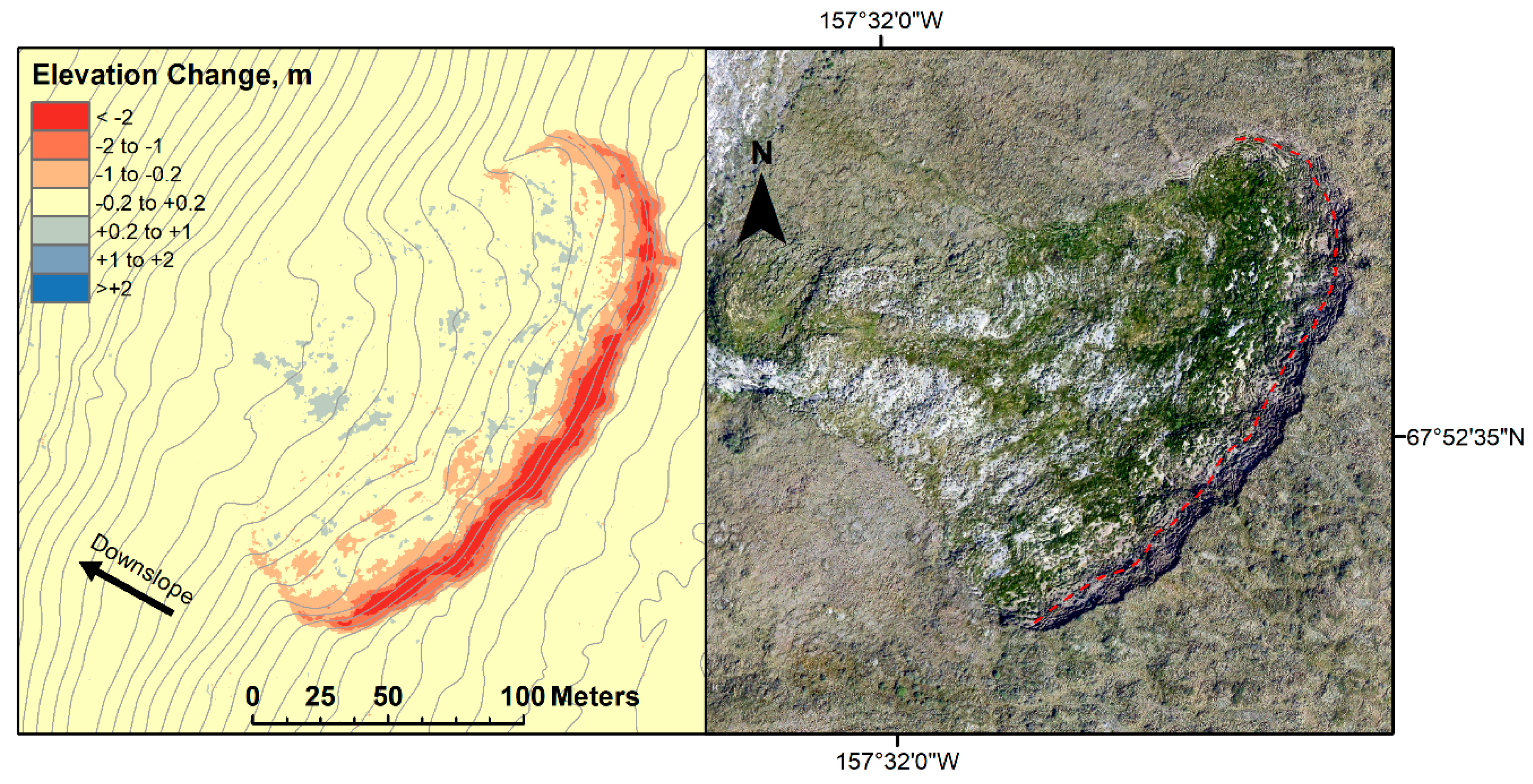
Retrogressive thaw slumps (RTS) in the Noatak National Preserve, Alaska. The contour map on the left (1 m contour interval), a result of this study, shows elevations in 2016 and the elevation change from 16 September 2013 to 11 July 2016. The orthophotograph on the right is from 2016, with the 2013 scarp position noted as a dashed red line. The volume changes in the upper subsidence zone (red, −) and nearby deposition zone (blue, +) were, for slump NOAT068: −19,216 m3 and +5959 m3 (31% of the subsidence volume); and for slump NOAT069: −7759 m3 and +2623 m3 (34% of the subsidence volume).
Figure 1.
Retrogressive thaw slumps (RTS) in the Noatak National Preserve, Alaska. The contour map on the left (1 m contour interval), a result of this study, shows elevations in 2016 and the elevation change from 16 September 2013 to 11 July 2016. The orthophotograph on the right is from 2016, with the 2013 scarp position noted as a dashed red line. The volume changes in the upper subsidence zone (red, −) and nearby deposition zone (blue, +) were, for slump NOAT068: −19,216 m3 and +5959 m3 (31% of the subsidence volume); and for slump NOAT069: −7759 m3 and +2623 m3 (34% of the subsidence volume).

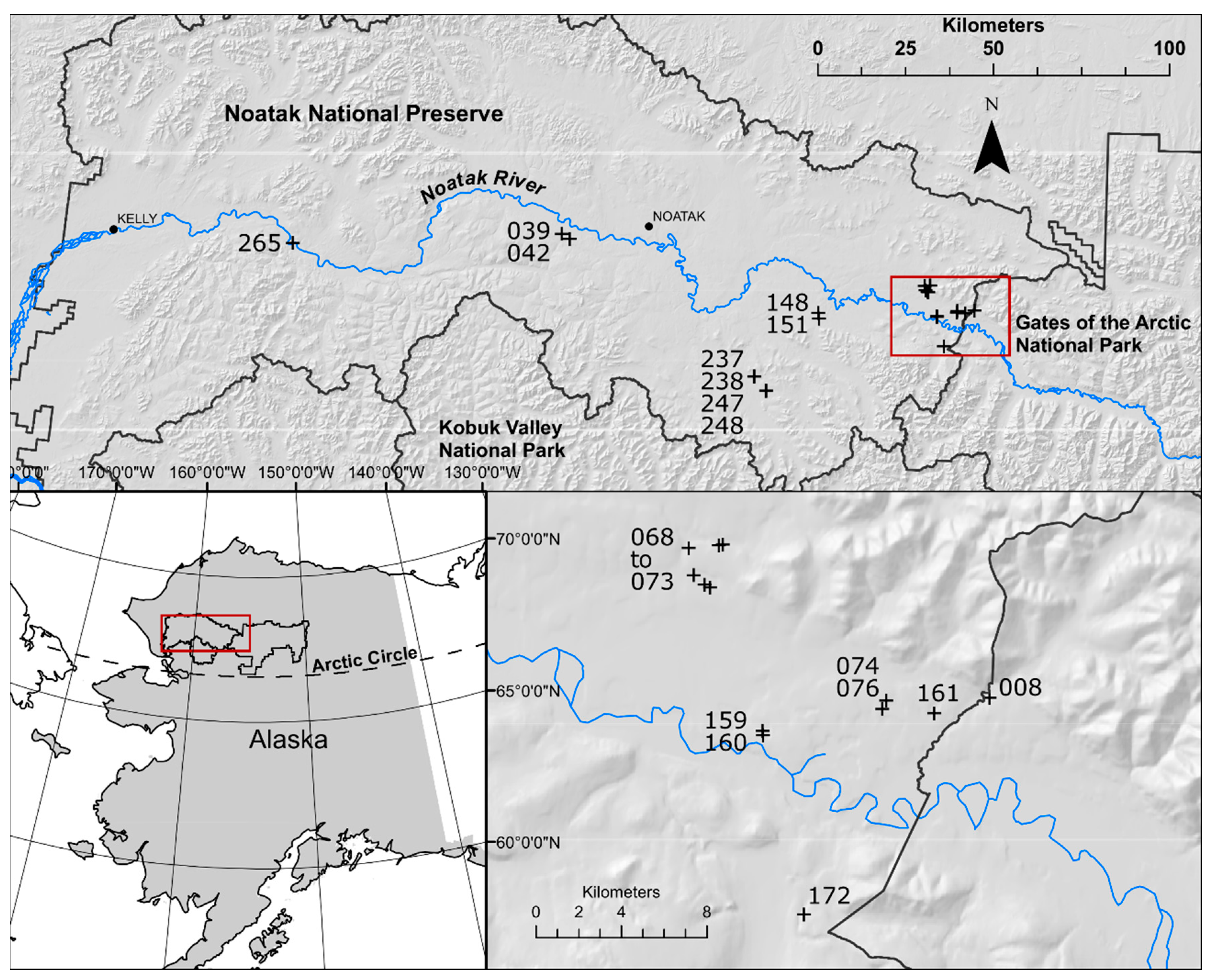
Figure 2.
Location of the study area. The study slumps are marked with a plus sign (+) and labeled with the three digits from the slump identifiers used in the text and tables. The inset maps show the overall location (lower left) and detail of the slump-rich portion of the eastern Noatak Valley (lower right). Locations of the Kelly and Noatak RAWS (weather stations) are also shown.

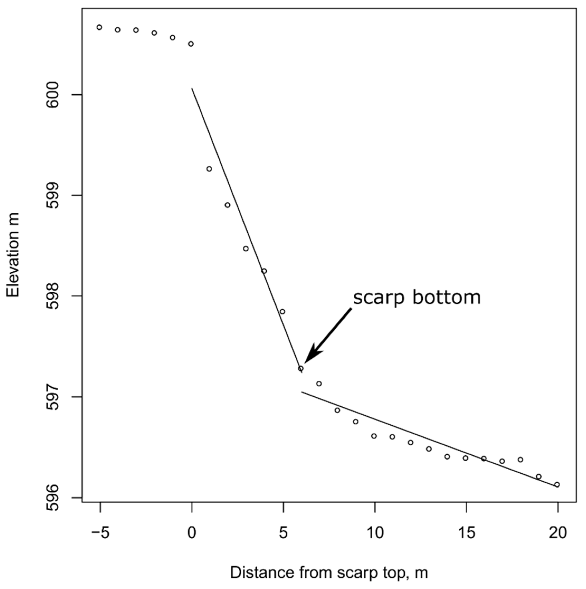
Figure 3.
Extraction of scarp height from a Digital Elevation Model (DEM). Elevations were extracted at 1-m intervals from a DEM along the slump centerline. The top of the scarp was located from the manually digitized slump perimeter. The bottom of the scarp was located by sequentially selecting trial breakpoints and fitting linear regressions to the elevations above and below. The breakpoint (labeled “scarp bottom”) resulting in the lowest combined mean square deviation for the two lines was accepted as the bottom of the scarp (data from slump NOAT070 in 2013).

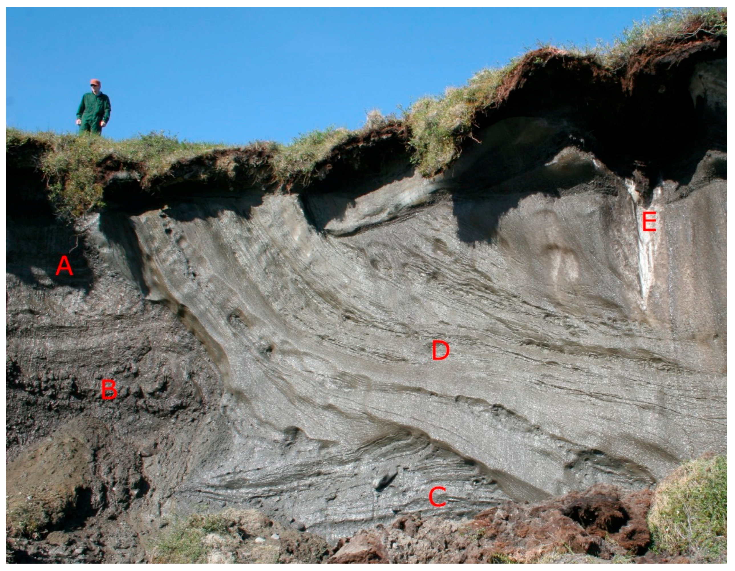
Figure 4.
Oblique aerial photograph of the main scarp and adjacent slump floor of slump NOAT070 on 19 July 2011. The main scarp was 4 to 5 m high and exposed about 1.5 m of dark glacial till (A) over light gray glacial ice (B). The shiny zone below the scarp (C) was viscous, water-saturated mud, while the dull-colored material (E) was compact sediment that would support a person’s weight. The main scarp position at the previous visit (22 June 2010) was just below the small ridge (D) that separates the liquid and solid zones of the floor.

Figure 5.
Exposure of ground ice from slump NOAT039. A—frozen loess, B—frozen glacial till, C—Pleistocene glacial ice (note the cobbles), D—Pleistocene ice wedge, E—Holocene ice wedge.
Figure 5.
Exposure of ground ice from slump NOAT039. A—frozen loess, B—frozen glacial till, C—Pleistocene glacial ice (note the cobbles), D—Pleistocene ice wedge, E—Holocene ice wedge.

Figure 6.
Exposure of the main scarp in slump NOAT265. The poorly sorted sediment in this exposure lacked obvious massive ice, but it contained enough ice to produce a zone of saturated mud at its base.
Figure 6.
Exposure of the main scarp in slump NOAT265. The poorly sorted sediment in this exposure lacked obvious massive ice, but it contained enough ice to produce a zone of saturated mud at its base.

Figure 7.
Slump areas vs. cumulative thaw degree-days (TDDs), (left) for large slumps with final areas greater than 2 to 7 ha; and (right) for small slumps with final areas of 0.5 to 2 ha. TDDs were measured at the Noatak RAWS and accumulated from an arbitrary start date of 1 January 2004. The vertical dashed lines mark winters (when TDD did not accumulate for multiple months), and the intervening thaw-season years are labeled. Curves are quadratic with regression coefficients in Table S6. The 3-digit numbers, coded by color, identify the slumps (Figure 2).

Figure 8.
Scarp position along the centerline vs. cumulative TDDs. TDDs were measured at the Noatak RAWS and accumulated from an arbitrary start date of 1 January 2004. The vertical dashed lines mark winters (when TDD did not accumulate for multiple months), and the intervening thaw-season years are labeled. Curves are quadratic with regression coefficients in Table S7. The 3-digit numbers, coded by color, identify the slumps (Figure 2).

Figure 9.
Scarp migration rate along the centerline vs. topographic slope at the scarp. The circle symbols are scaled to the escarpment height, with examples labeled with height in meters to illustrate the scale. Symbols are colored by the type of ground ice observed in the scarp exposures: blue—glacial ice; green—wedge ice, with or without glacial ice below; black—no massive ice observed in the exposure (slump NOAT265); and brown—poor exposures prevented examination of ground ice.

Figure 10.
Topographic cross-sections of slump NOAT070, 2010–2016.

Figure 11.
Scarp migration rate vs. orientation of the scarp. Scarp migration rates for sequential observation dates of a single slump are connected by lines of a single color.
Figure 11.
Scarp migration rate vs. orientation of the scarp. Scarp migration rates for sequential observation dates of a single slump are connected by lines of a single color.

Figure 12.
Main scarp of slump NOAT151 in an area that had previously slumped and revegetated. About 1.5 m of reworked glacial till (A) was over debris-rich glacial ice (B). The mud-water slurry formed by melt at the scarp is below (C).
Figure 12.
Main scarp of slump NOAT151 in an area that had previously slumped and revegetated. About 1.5 m of reworked glacial till (A) was over debris-rich glacial ice (B). The mud-water slurry formed by melt at the scarp is below (C).

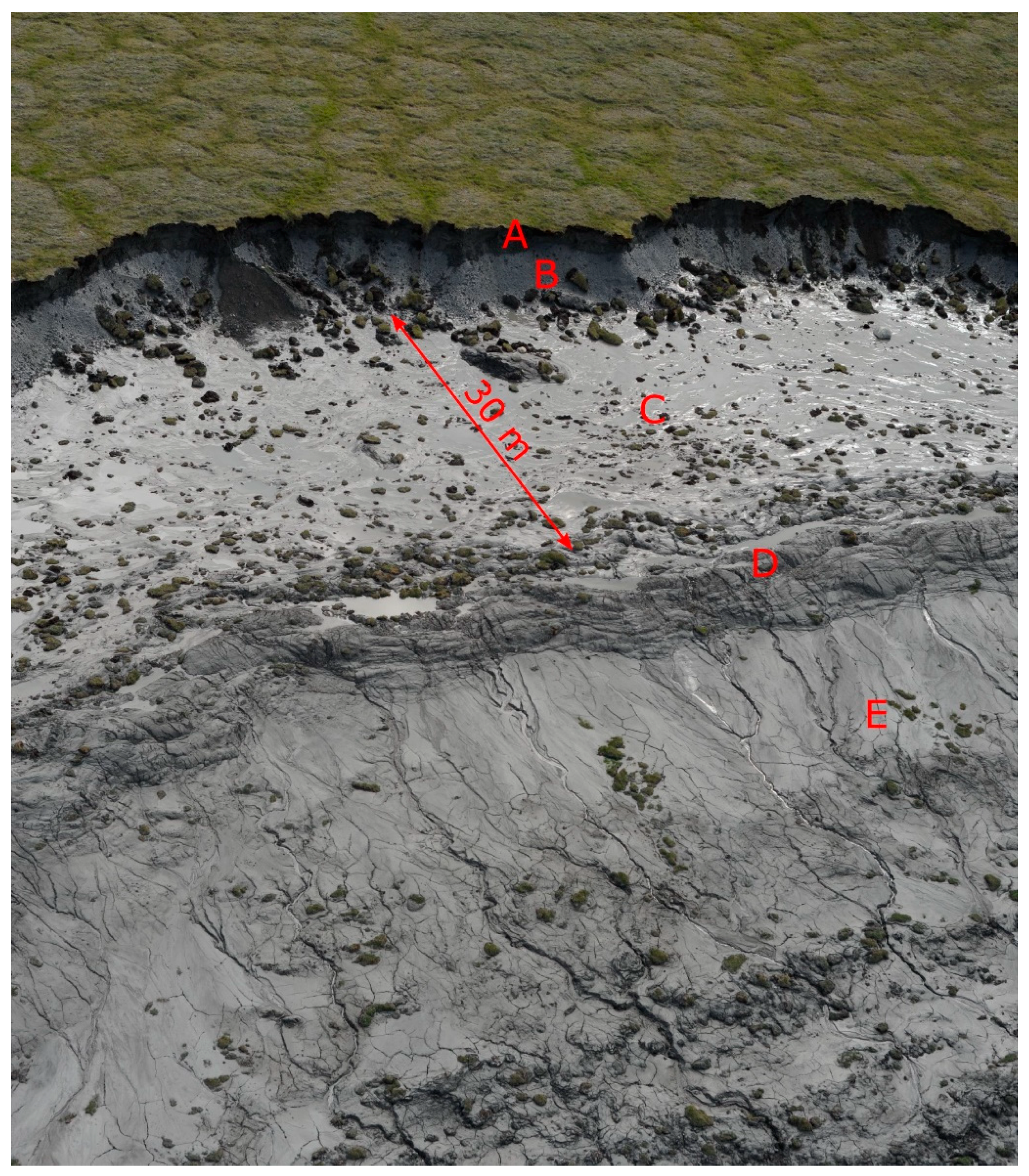
Figure 13.
Orthophotograph of retrogressive thaw slump (RTS) NOAT265 and associated scars from the preceding active-layer detachments (ALD); photograph from 19 August 2008 by Tom George. The slump was expanding up the two ALD on the left. The dashed lines show the position of the main scarp in the ALD scars. The photograph is natural color; the reddish tones are due to early fall vegetation senescence.

Figure 14.
Retrogressive thaw slump NOAT070. The contour map on the left (1 m contour interval) shows elevations in 2016 and the elevation change from 16 September 2013 to 11 July 2016. The orthophotograph on the right is from 2016, with the 2013 scarp position noted. The volume change in the upper subsidence zone (red) was −15062 m3 and in the nearby deposition zone (blue) +4951 m3 (33% of the subsidence volume).
Figure 15.
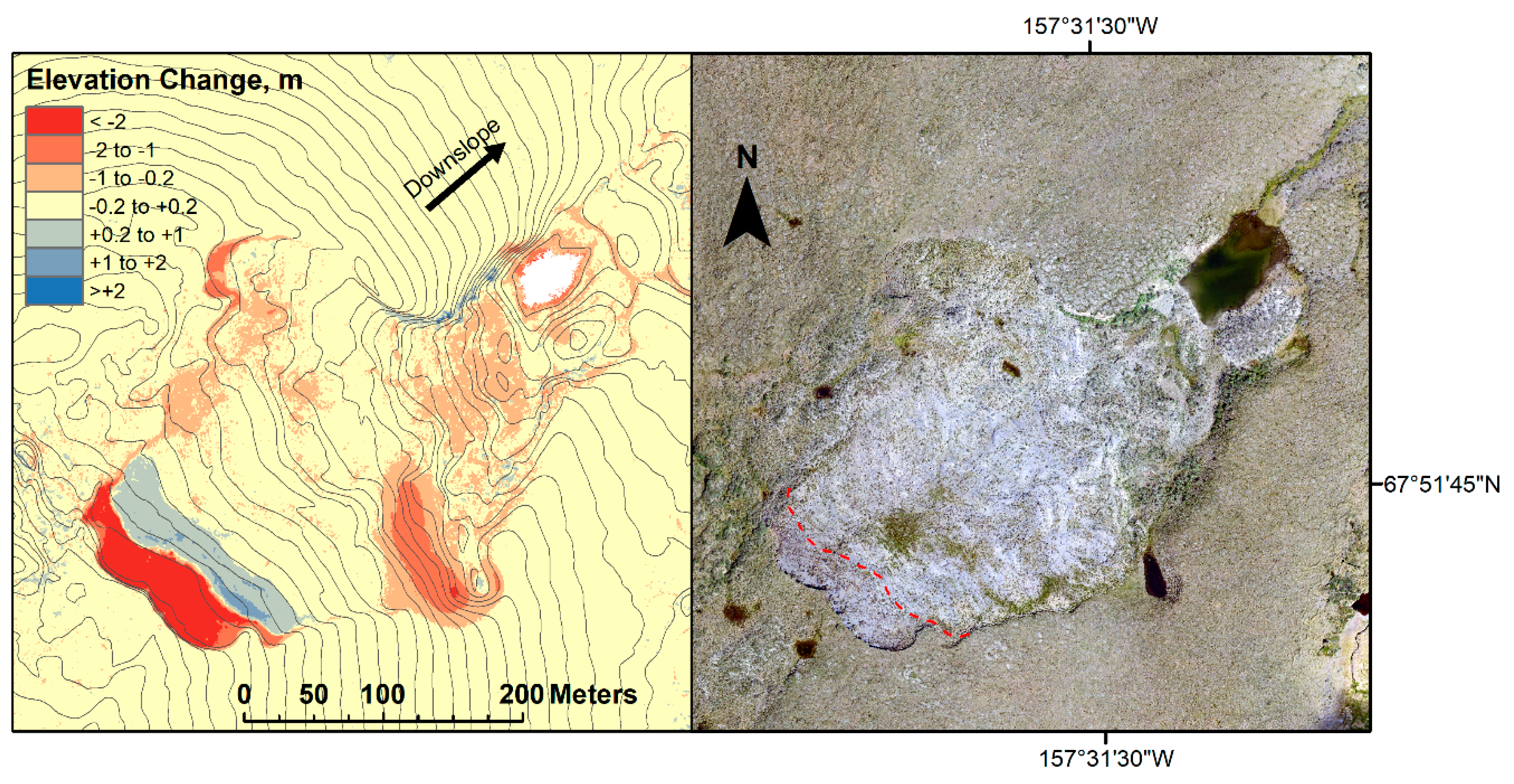
Retrogressive thaw slump NOAT148. The contour map on the left (1 m contour interval) shows elevations in 2016 and the elevation change from 16 September 2013 to 11 July 2016. The orthophotograph on the right is from 2016, with the 2013 scarp position noted. The volume change in the upper subsidence zone (red) was −6529 m3.
Figure 15.
Retrogressive thaw slump NOAT148. The contour map on the left (1 m contour interval) shows elevations in 2016 and the elevation change from 16 September 2013 to 11 July 2016. The orthophotograph on the right is from 2016, with the 2013 scarp position noted. The volume change in the upper subsidence zone (red) was −6529 m3.

Figure 16.
Retrogressive thaw slump NOAT151. The contour map on the left (1 m contour interval) shows elevations in 2016 and the elevation change from 16 September 2013 to 11 July 2016. The orthophotograph on the right is from 2016, with the 2013 scarp position noted. The volume changes in the upper subsidence zone (red) −12732 m3 and nearby deposition zone (blue) +3308 m3 (26% of the subsidence volume).

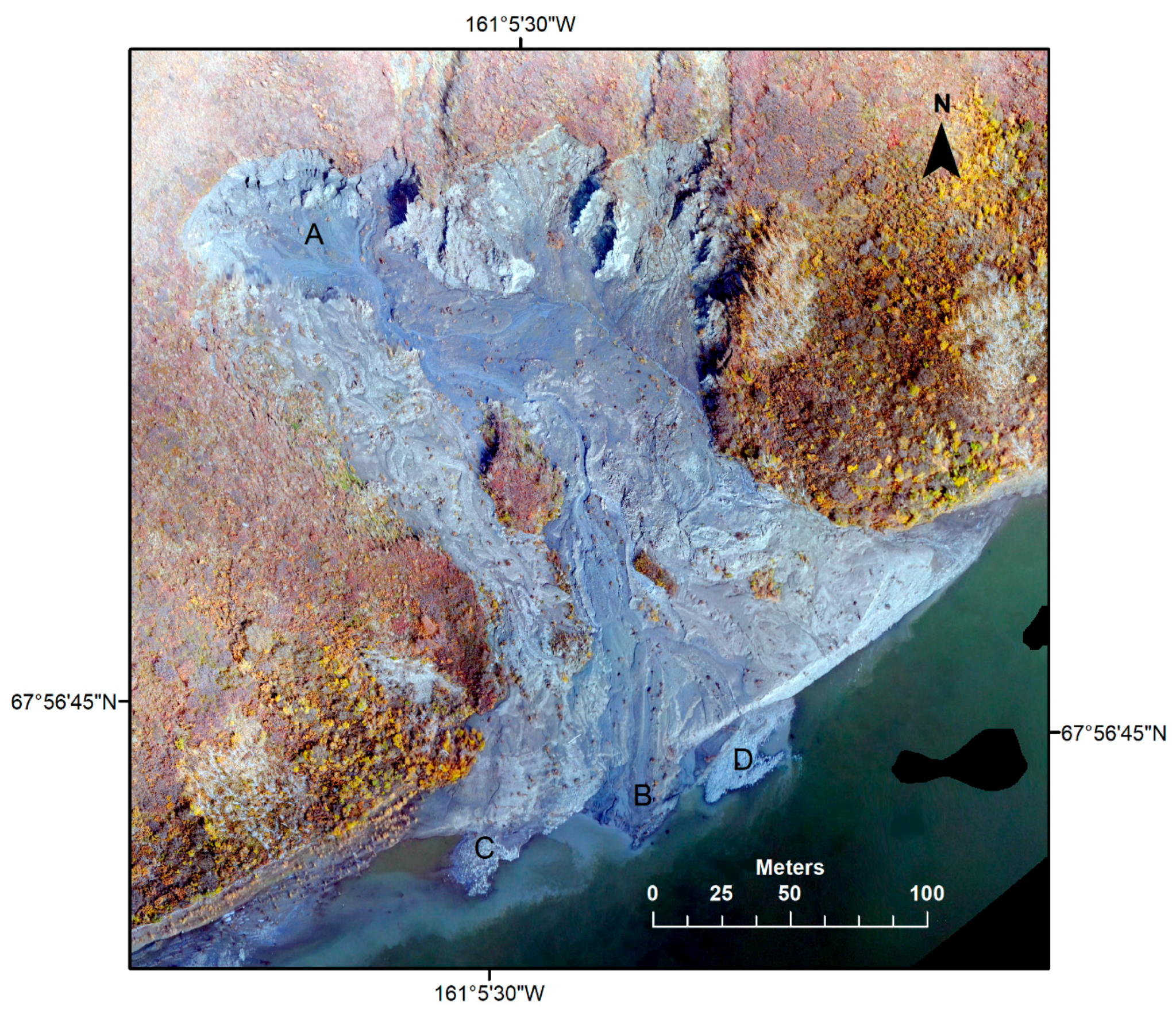
Figure 17.
Orthophotograph of slump NOAT265 from photographs taken on 11 September 2012. Note the active channels transporting sediment from the wet area near the main scarp (A) to an active depositional fan in the Noatak River (B). Inactive fans at (C) and (D) mark the terminations of previous channels.


Table 1.
Statistics for difference between 2013 and 2016 DEMs in a buffer zone outside the slump 1.
| Slump ID | Pixel Count | Mean Difference, m | Std Deviation of Difference, m |
|---|---|---|---|
| NOAT068-69 | 1837835 | −0.415 | 0.052 |
| NOAT070 | 1018278 | −0.487 | 0.069 |
| NOAT148 | 753154 | −0.254 | 0.050 |
| NOAT151 | 822979 | −0.286 | 0.076 |
1 DEMs were created using vertical aerial photographs, with airborne GPS for georeferencing. The buffer zones were 10 to 50 m outside of the slump perimeters and presumed to have been unchanged.
Table 2.
Slump ground ice, geologic setting, and growth rate characteristics along the centerline for an example year. 1
Table 2.
Slump ground ice, geologic setting, and growth rate characteristics along the centerline for an example year. 1
| Ground Ice 2 | Slump | Surficial Geology 3 | Neighboring Waterbody 4 | Year 1 | Year 2 | Area, ha | Centerline Scarp Retreat Rate, m yr−1 | Scarp Height at Centerline, m |
|---|---|---|---|---|---|---|---|---|
| g | GAAR008 | id2 | Stream, 100 m | 2011 | 2012 | 1.3 | 5.3 | 1.8 |
| g | NOAT068 | id1 | Stream | 2011 | 2013 | 3.7 | 23.6 | 3.9 |
| g | NOAT069 | id1 | Stream, 3 m | 2011 | 2012 | 1.7 | 35.3 | 2.8 |
| g | NOAT070 | id1 | Stream | 2011 | 2012 | 5.1 | 28.5 | 3.6 |
| g | NOAT074 | id2 | Lake | 2011 | 2012 | 1.4 | 14.2 | 2.0 |
| g | NOAT076 | id2 | Lake | 2011 | 2012 | 1.3 | 11.4 | 2.5 |
| g | NOAT159 | id2 | Lake | 2011 | 2012 | 0.8 | 1.6 | 1.3 |
| g | NOAT160 | id2 | Lake | 2011 | 2012 | 1.0 | 1.3 | 1.3 |
| g | NOAT161 | id2 | Lake | 2011 | 2012 | 1.6 | 11.6 | 2.3 |
| g | NOAT237 | igl1 | Lake | 2011 | 2012 | 1.5 | 18.6 | 2.0 |
| n | NOAT265 | tg? | Stream | 2011 | 2012 | 3.4 | 20.3 | 12.2 |
| p | NOAT071 | id1 | Lake | 2012 | 2013 | 0.9 | 1.6 | 2.1 |
| p | NOAT072 | id1 | Lake | 2012 | 2013 | 0.7 | 0.9 | 1.7 |
| p | NOAT073 | id1 | Lake | 2012 | 2013 | 0.7 | 1.1 | 1.3 |
| p | NOAT238 | igl1 | Lake | 2011 | 2012 | 0.6 | 1.2 | 2.6 |
| p | NOAT247 | igl1 | Lake | 2011 | 2013 | 0.9 | 0.9 | 3.4 |
| p | NOAT248 | igl1 | Lake | 2011 | 2013 | 1.0 | 1.9 | 1.4 |
| w | NOAT172 | id2 | Stream, 100 m | 2011 | 2012 | 1.3 | 5.8 | 7.2 |
| wg | NOAT039 | id1 | Lake | 2011 | 2012 | 4.8 | 3 | 8.6 |
| wg | NOAT042 | id1 | Lake | 2011 | 2012 | 1.9 | 5.3 | 4.9 |
| wg | NOAT148 | id1 | Stream, 10 m | 2012 | 2013 | 2.3 | 7.3 | 5.1 |
| wg | NOAT151 | id1 | Stream, 100 m | 2011 | 2012 | 5.2 | 13.3 | 3.9 |
1 Data beginning in 2011 if available, otherwise 2012. 2 g—glacial ice, w—wedge ice, wg—wedge and glacial ice, n—massive ice not visible, p—poor exposure. 3 From Hamilton [35]. id1—Itkillik phase I glacial drift, id2—Itkillik phase II glacial drift, igl1—Itkillik phase I glaciolacustrine deposits, tg?—possible Pleistocene terrace gravel. 4 Type of water body at the foot of the slope. The distance from the end of the area obviously disturbed by the slump to the water body is given; where the distance is omitted, the disturbed area contacted the water body directly.
Table 3.
Initiation years and previous slumping activity on the study slumps.
| Slump | Year of First Detection | Year of Area Growth Curve X-Intercept 3 | Observed Area Change, % of Final 4 | |
|---|---|---|---|---|
| by SAR 1 | by Landsat and Aerial Photo 2 | |||
| GAAR008 | ND | 2005 | 2005 | 39 |
| NOAT039 | pre-1980 | pre-1980 | 2003 | 49 |
| NOAT042 | 2004 | pre-1980; 2005 | 2003 | 54 |
| NOAT068 | 2005 | 2005 | 2005 | 64 |
| NOAT069 | 2005 | 2006 | 2006 | 72 |
| NOAT070 | 2004 | pre-1980; 2005 | 2006 | 62 |
| NOAT071 | 1978–1997 | 1995 | pre-2000 | 7 |
| NOAT072 | 2005 | 2006 | 2004 | 35 |
| NOAT073 | 2004 | 2007 | 2003 | 26 |
| NOAT074 | 2004 | 2008 | 2007 | 69 |
| NOAT076 | 2004 | 2006 | 2006 | 44 |
| NOAT148 | 2004 | 2005 | 2004 | 46 |
| NOAT151 | 1998 | pre-1980; 2004 | 2002 | 39 |
| NOAT159 | 2004 | 2007 | 2007 | 45 |
| NOAT160 | 2004 | 2006 | 2005 | 31 |
| NOAT161 | ND | 2005 | 2005 | 36 |
| NOAT172 | ND | 2005 | 2004 | 35 |
| NOAT237 | ND | pre-1980; 2006 | 2006 | 67 |
| NOAT238 | ND | pre-1980; 2004 | 2004 | 29 |
| NOAT247 | ND | pre-1980; 2005 | pre-2000 | 9 |
| NOAT248 | 2004 | pre-1980; 2005 | pre-2000 | 11 |
| NOAT265 | ND | 2005 | 2005 | 60 |
1 From Balser [13], who used synthetic aperture radar images with approximately 25 m resolution to identify the timing of slump initiation. ND—no data. 2 Based on Landsat images, c. 1980 Alaska High-Altitude (AHAP) color-infrared aerial photographs, and c. 1955 panchromatic aerial photographs (this study). The second date refers to the time of reactivation after a period of stability prior to 2004. 3 X-intercept of quadratic curves fit to area vs. thaw degree-day plot (Figure 7 and Table S6). 4 Change in area between the first and last samples in this study (2008–2016 for most slumps), as a percentage of the area at the last sample.
© 2018 by the authors. Licensee MDPI, Basel, Switzerland. This article is an open access article distributed under the terms and conditions of the Creative Commons Attribution (CC BY) license (http://creativecommons.org/licenses/by/4.0/).
Share and Cite
MDPI and ACS Style
Swanson, D.K.; Nolan, M. Growth of Retrogressive Thaw Slumps in the Noatak Valley, Alaska, 2010–2016, Measured by Airborne Photogrammetry. Remote Sens. 2018, 10, 983. https://doi.org/10.3390/rs10070983
AMA Style
Swanson DK, Nolan M. Growth of Retrogressive Thaw Slumps in the Noatak Valley, Alaska, 2010–2016, Measured by Airborne Photogrammetry. Remote Sensing. 2018; 10(7):983. https://doi.org/10.3390/rs10070983
Chicago/Turabian StyleSwanson, David K., and Matt Nolan. 2018. "Growth of Retrogressive Thaw Slumps in the Noatak Valley, Alaska, 2010–2016, Measured by Airborne Photogrammetry" Remote Sensing 10, no. 7: 983. https://doi.org/10.3390/rs10070983
Note that from the first issue of 2016, this journal uses article numbers instead of page numbers. See further details here.