Article

High-Spatial Resolution Monitoring of Phycocyanin and Chlorophyll-a Using Airborne Hyperspectral Imagery

1
School of Urban and Environmental Engineering, Ulsan National Institute of Science and Technology, Ulsan 689-798, Korea
2
Department of Atmospheric Science and Engineering, Ewha Womans University, Ewha-Yeodae-Gil 52, Seodaemoon-Gu, Seoul 03760, Korea
3
Yeongsan River Environmental Research Center, National Institute of Environmental Research, Gwangju 61011, Korea
4
Water Quality Assessment Research Division, National Institute of Environmental Research, Environmental Research Complex, Incheon 22689, Korea
5
GEOSTROY Inc., Hwa-gok-lo 68-82, Gangseo-Gu, Seoul 07566, Korea
6
School of Civil and Environmental Engineering, Konkuk University, Neumgdong-Ro 120, Gangjin-Gu, Seoul 05029, Korea
*
Authors to whom correspondence should be addressed.
Remote Sens. 2018, 10(8), 1180; https://doi.org/10.3390/rs10081180
Submission received: 14 June 2018 / Revised: 20 July 2018 / Accepted: 21 July 2018 / Published: 26 July 2018

Abstract

:
Hyperspectral imagery (HSI) provides substantial information on optical features of water bodies that is usually applicable to water quality monitoring. However, it generates considerable uncertainties in assessments of spatial and temporal variation in water quality. Thus, this study explored the influence of different optical methods on the spatial distribution and concentration of phycocyanin (PC), chlorophyll-a (Chl-a), and total suspended solids (TSSs) and evaluated the dependence of algal distribution on flow velocity. Four ground-based and airborne monitoring campaigns were conducted to measure water surface reflectance. The actual concentrations of PC, Chl-a, and TSSs were also determined, while four bio-optical algorithms were calibrated to estimate the PC and Chl-a concentrations. Artificial neural network atmospheric correction achieved Nash-Sutcliffe Efficiency (NSE) values of 0.80 and 0.76 for the training and validation steps, respectively. Moderate resolution atmospheric transmission 6 (MODTRAN 6) showed an NSE value >0.8; whereas, atmospheric and topographic correction 4 (ATCOR 4) yielded a negative NSE value. The MODTRAN 6 correction led to the highest R2 values and lowest root mean square error values for all algorithms in terms of PC and Chl-a. The PC:Chl-a distribution generated using HSI proved to be negatively dependent on flow velocity (p-value = 0.003) and successfully indicated cyanobacteria risk regions in the study area.

Graphical Abstract

1. Introduction

Severe algal blooms, mainly caused by anthropogenic effects, are an ongoing cause of water quality problems in inland waters globally [1,2,3,4,5,6]. Massive nutrient loads from both point and non-point sources accelerate the growth and biomass production of algae [7]. In Korea, increases in water retention times because of the construction of multi-functional weirs contributes to the frequent formation of cyanobacterial blooms [8,9,10]. Baekje Weir along the Geum River, for example, has recently received increased attention because of water quality issues caused by frequent outbreaks of severe cyanobacterial blooms [11,12]. These have caused water quality degradation in the weir, which can lead to adverse effects on human health [13,14].
Remote-sensing techniques are useful in the detection of algal blooms because they can detect algae over large areas at a high time resolution [15,16,17,18,19,20,21,22,23,24,25,26,27]. Specifically, many bio-optical algorithms that use remotely sensed data have been developed to estimate the concentrations of algal pigments such as chlorophyll-a (Chl-a) and phycocyanin (PC) [28,29,30,31,32]. PC and Chl-a concentrations have been estimated using various apparent optical property (AOP) algorithms [33,34,35,36] and inherent optical property (IOP) algorithms [30,31,37,38,39]. AOP algorithms utilize water surface reflectance to estimate the algal concentration using multiple reflectance bands. The authors of [17] and [28] introduced a two-band ratio algorithm and three-band ratio algorithm for Chl-a and PC estimation, respectively. IOP algorithms use absorption and the back scattering coefficient for estimation of algal pigments. The authors of [29,30] estimated Chl-a and PC concentration using the ratio of the absorption coefficient and specific absorption coefficient.
Hyperspectral imagery (HSI) provides a spatially detailed information map of high spectral resolution. This high resolution allows hyperspectral images to be used for the identification and analysis of sophisticated spatial and spectral information [40,41,42,43,44]. Accurate retrieval of algal biomass from a hyperspectral image requires an atmospheric correction to remove atmospheric interference. Commercial atmospheric software packages such as atmospheric and topographic correction (ATCOR) [45] are often used to correct the images. Thiemann and Kaufmann [46] implemented atmospheric correction of hyperspectral images using ATCOR to generate maps of Secchi disk transparency and Chl-a concentration. Alternatively, users can perform the atmospheric correction themselves using the Moderate resolution atmospheric transmission (MODTRAN) software, which provides atmospheric correction parameters [47]. Giardino et al. [48] used MODTRAN to perform atmospheric correction of HSI to retrieve the Chl-a of an inland water. Furthermore, machine learning techniques have been introduced to correct atmospheric effects using observed atmospheric parameters [49,50,51].
Previous studies have used various atmospheric correction methods either to achieve good correction performance [22,52,53,54,55,56] or simply to estimate the target [44,57,58,59,60]. However, few studies have quantitatively analyzed the dependence of the atmospheric correction performance on the correction method [61]. In particular, algal detection studies, which consider the effect of atmospheric correction on PC and Chl-a concentration estimates, have been rarely completed. Moreover, when preprocessed hyperspectral images provide an algal distribution map, the concentration level and spatial distribution of algae are influenced by environmental factors such as water temperature, nutrients, and water retention time. The authors of [9,62,63] showed the distribution of algae is mainly affected by influencing factors such as hydrodynamic patterns. Thus, identifying the cause of an algal bloom is important after producing an algal distribution map.
Therefore, the objectives of this study were to (1) implement atmospheric correction of hyperspectral images using MODTRAN 6, ATCOR 4, and Artificial Neural Network (ANN); (2) develop bio-optical algorithms to estimate PC and Chl-a concentration using the corrected hyperspectral images; (3) identify the influence of the atmospheric correction on PC and Chl-a quantification; and (4) evaluate the algal distribution with hydrodynamic patterns.

2. Materials and Methods
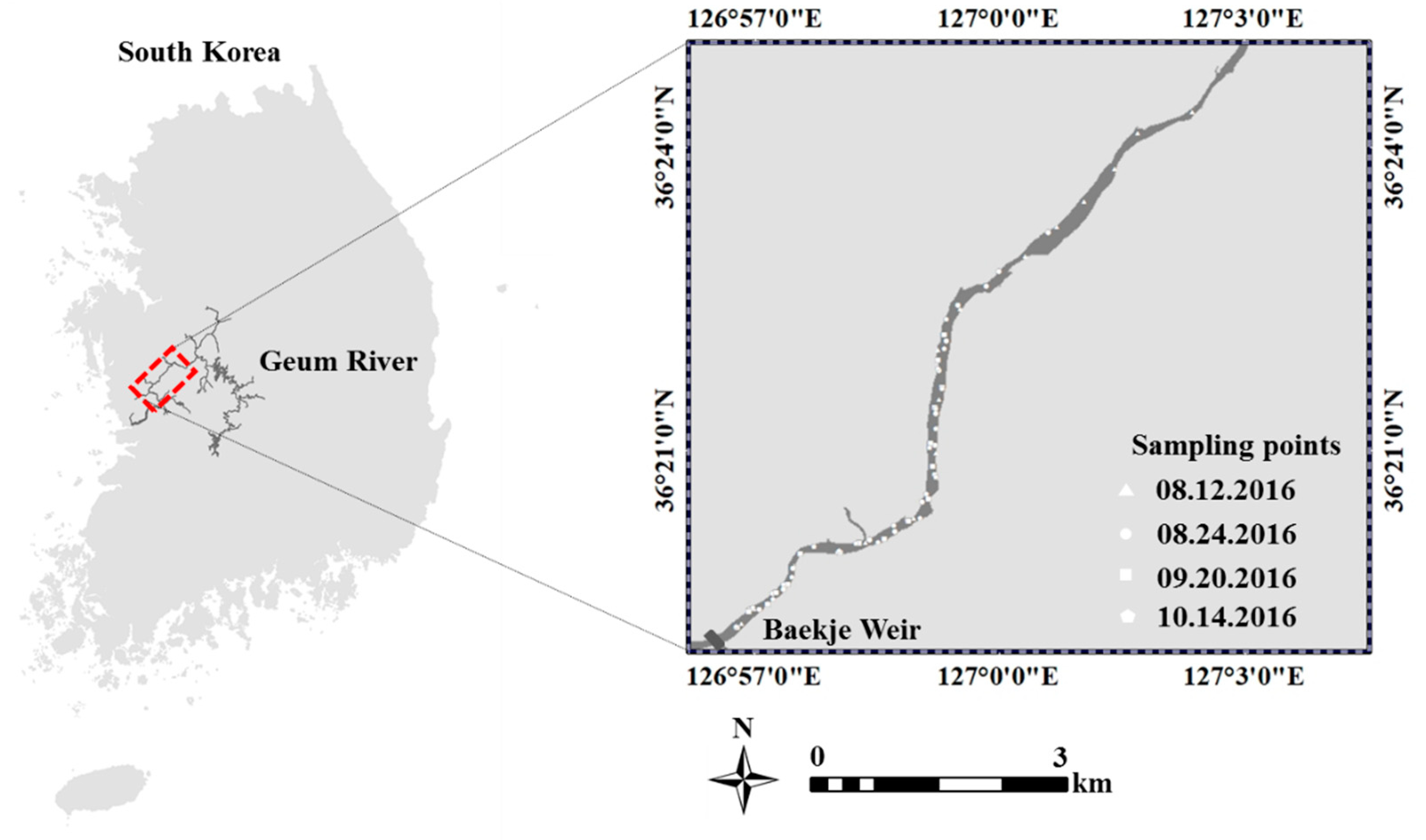
2.1. Study Area

The Baekje Reservoir (36°32′N 126°94′E) is an artificial weir in the Geum River in South Korea (Figure 1). The Geum River has a total length of 395 km. It has three man-made weirs (the Baekje, Gongju, and Saejong reservoirs) and one dam (the Daechung dam). The distance between the Baekje and Gongju weirs along the river is 23 km, over which the width is 50 m and the average water depth is 4 m. The Baekje Weir has a length of 331 m and height of 5.3 m, and a total storage capacity of 24 × 106 m3. The stored water is used for both domestic and agricultural purposes.

2.2. Remote Sensing of PC and Chl-a Pigment

Figure 2 shows the research scheme employed in this study. The diagram is divided into four parts: (a) data collection from field and laboratory measurements were conducted; (b) atmospheric correction of hyperspectral images was performed using MODTRAN 6 and ATCOR 4 software; (c) atmospheric correction parameters generated by MODTRAN 6 were used in an ANN-simulated atmospheric correction; and (d) the corrected reflectance values from MODTRAN 6, ATCOR 4, and ANN were applied to build bio-optical algorithms for the estimation of PC and Chl-a concentrations. Finally, the bio-optical algorithms were used to generate the spatial and temporal distribution of the PC and Chl-a concentrations and identify the influence of the atmospheric correction on the PC and Chl-a quantification.

2.2.1. Water Sampling and Experimental Work

Field campaigns were conducted on 12 August, 24 August, 20 September, and 14 October 2016 (Table 1). During the sampling period, optical data and water samples were collected at 74 monitoring stations.
The measured radiance and irradiance data were used to calculate the remote-sensing reflectance while the PC and Chl-a were quantified in the water samples. Cyanobacteria contain the PC pigment, which harvests light through photosynthesis [64]. The representative absorption band for PC is around 620 nm [65]. For PC extraction, water samples were concentrated using a phytoplankton net with a 20-μm mesh size. The pre-concentration water volume varied from 10 L to 45 L. The concentrated water was stored in a 100-mL wide-necked bottle and kept cool in a box with ice. The water samples were analyzed within 24 h in the laboratory. PC was extracted by applying the freezing and thawing method [66]. The detailed experimental procedures of PC extraction are described in [38]. Two liters of water samples were collected for Chl-a analysis and analyzed within 24 h. The extraction of Chl-a followed a standard method [67]. Specific information regarding Chl-a analysis is presented in [38]. A standard method was used for the analysis of total suspended solid (TSS) concentration. A glass microfiber filter (GF/C, WHATMAN Inc., Piscataway, NJ, USA) was preferentially washed with deionized water and dried in a desiccator. Before filtration, the weight of the filter was measured using an analytical balance (EX224, OHAUS Inc., Parsippany, NJ, USA). After the filtration of the water samples, the used filter papers were placed in a drying oven (DO-150, HYSC Inc., Seoul, Korea) for 2 h. Finally, the dried filters were weighed using the analytical balance. The TSS concentration was calculated using the following equation:
  Total   Suspended   Solid   ( mg   L 1 ) = ( F a F b ) × 1000 V      
where, Fa is the weight of the filter after filtration (mg), Fb is the weight of the filter before filtration (mg), and V is the volume (mL) of the sample.
The absorption coefficient of phytoplankton was measured using light transmission measurement. This measurement was able to obtain the phytoplankton absorption coefficient without the signal of a non-algal particle by performing bleaching processing. A more detailed method of absorption coefficient measurement was followed by [38].

2.2.2. Field Optical and Hyperspectral Reflectance Data

A FieldSpec HandHeld2 hand-held spectroradiometer (ASD, Inc., Longmont, CO, USA) was used to collect radiance and irradiance data. The spectroradiometer has a band range of 325 nm to 1075 nm and a 3-nm spectral resolution. The device has a 25-degree field-of-view. This spectroradiometer collects sky irradiance (Er) using a cosine detector fore-optic, and water surface radiance (Lw) and sky radiance (Ls) using a bare fiber fore-optic. Optical sampling requires a specific position of the spectroradiometer with 130–135 degrees of azimuth angle and 40–45 degrees of zenith angle. This position minimizes ambient interferences such as the sun glint and shading effects [29]. The remote-sensing reflectance uses the ratio of irradiance to radiance as follows:
  R rs ( λ , 0 + ) = L w ( λ , 0 + ) 0.025 L s ( λ ) E r ( λ )      
where L w ( λ , 0 + ) is the water leaving radiance, L s ( λ ) is the downwelling sky radiance, E r ( λ ) is the downwelling sky irradiance, R rs ( λ , 0 + ) is the remote-sensing reflectance, and 0+ denotes the water surface. Detailed information on the remote-sensing spectra is presented in [38].
Table 1 presents a summary of the field campaigns. Four airborne monitoring campaigns along the Geum River were implemented simultaneously with the ground-based monitoring. The airborne campaigns were performed by ASIA Aero Survey co., Ltd. (Seoul, Korea) using an AISA Dual airborne hyperspectral sensor. The sensor direction is perpendicular to the ground. The altitude of the aircraft was 3 km and the flying time was between two and three hours, beginning at 8:30 a.m. The hyperspectral image has 127 wavelength bands from 404 nm to 996 nm. The image has a spectral resolution of 4 nm to 5 nm and a spatial resolution of 2 m × 2 m. This study applied atmospheric correction using ATCOR 4, MODTRAN 6, and an ANN.

2.2.3. Atmospheric Correction

ATCOR is a commercial software package that was developed during the 1990s [45,68]. The main features of this software are correction of the topographic and adjacency effect and spectral smoothing [45]. ATCOR 4 is a user-friendly software for atmospheric correction of HSI. Its ease of use stems from the straightforward and fast simulation [69].
MODTRAN was developed by Spectral Science, Inc. (Burlington, MA, USA) and the Air Force Research Laboratory (AFRL) [47]. The MODTRAN code solves the radiative transfer function to generate physical parameters related to atmospheric correction such as transmittance and spherical albedo. MODTRAN version 6 has a graphical user interface (GUI), making this software user friendly.
This study implemented atmospheric correction using the ANN to simulate ρ surf . Detailed descriptions of the atmospheric correction using ATCOR 4, MODTRAN 6, and ANN are presented in Appendix A in the Supplementary Material.

2.2.4. Bio-Optical Algorithms for Determination of PC and Chl-a Concentration

This study estimated PC and Chl-a concertation using four bio-optical algorithms, two AOP algorithms, and two IOP algorithms, as follows.

AOP Algorithm

The AOP algorithm is based on the following remote-sensing reflectance:
  R r s ( λ ) = 0.54 ( f q b ( λ ) a ( λ ) + b ( λ ) )    
where R r s ( λ ) is the remote-sensing reflectance on the water surface, f is the geometric light factor, q is the light distribution factor, b ( λ ) is the backscattering coefficient, and a ( λ ) is the absorption coefficient.
This study used either two or three bands to estimate PC and Chl-a concentration. The first algorithm used was the two-band ratio algorithm [17,37,70,71,72], which is referred to as band ratio (2) in this text. Band ratio (2) estimates the PC concentration as follows:
  P C   ( mg   m 3 ) R r s ( 708 ) R r s ( 622 )  
  C h l a   ( mg   m 3 ) R r s ( 708 ) R r s ( 660 )    
where R r s ( 708 ) is the reflectance at 708 nm, R r s ( 660 ) is the reflectance at 660 nm, and R r s ( 622 ) is the reflectance at 622 nm.
The second algorithm used was the three-band ratio algorithm [28], which is referred to as the band ratio (3) in this manuscript. PC concentration was estimated by band ratio (3) using the following equations:
  P C   ( mg   m 3 ) ( 1 R r s ( 622 ) 1 R r s ( 708 ) ) · R r s ( 755 )    
  C h l a   ( mg   m 3 ) ( 1 R r s ( 660 ) 1 R r s ( 708 ) ) · R r s ( 755 )    
where R r s ( 755 ) is the reflectance at 755 nm.

IOP Algorithm

The IOP algorithm mainly uses absorption and b ( λ ) by rearranging Equation (4) in terms of a ( λ ) . Many studies have used the ratio form to retrieve a ( λ ) because this allows the removal of geometric and ambient light effects, assuming these effects are independent of wavelength [29]. The a ( λ ) equation is classified according to whether b ( λ ) is wavelength-dependent or not. Simis et al. [31] and Duan et al. [37] suggested the following formulation for the a ( λ ) equation with a wavelength-independent b ( λ ) :
  a ( λ a ) = R r s ( λ w ) R r s ( λ a ) ( a ( λ ) b ) b    
where λ a is the wavelength for the phytoplankton pigment (i.e., Chl-a or PC) and λ w is the wavelength for water.
Li et al. [29,30] introduced the following definition of a ( λ ) with a wavelength-dependent absorption coefficient:
  a ( λ a ) = ( R r s ( λ w ) b ( λ a ) ( a w ( λ w ) + b ( λ w ) ) R r s ( λ a ) b ( λ w ) ) b ( λ a ) a w ( λ a )    
where a w is the absorption coefficient of water referred to by [73]. The expression for the PC and Chl-a concentrations uses both the absorption coefficient and the specific absorption coefficient as follows:
  P C   ( mg   m 3 ) = a ( λ p c ) a * ( λ p c )  
  C h l a   ( mg   m 3 ) = a ( λ c h l a ) a * ( λ C h l a )    
where λ p c is the PC wavelength, a * ( λ p c ) is the specific absorption coefficient of PC (m2 mg−1), λ c h l a is the Chl-a wavelength, and a * ( λ c h l a ) is the specific absorption coefficient of Chl-a (m2 mg−1). A more detailed description of the IOP algorithm for the determination of PC and Chl-a can be found in [29,30,31,32].
The IOP algorithm requires many empirical parameters as well as wavelength bands that accurately reflect optical properties of the water body. This study optimized the Simis algorithm and Li algorithm using the multi-objective optimization, resulting in 622 nm for PC and 660 nm for Chl-a [38]. The band ratio (2), band ratio (3), Simis, and Li algorithms were applied to images which had atmospheric correction completed by MODTRAN 6, ATCOR 4, or ANN.

2.3. Performance Evaluation

Nash-Sutcliffe efficiency (NSE) and the root mean square error (RMSE) were used to evaluate the performances of the atmospheric correction, optimized bio-optical algorithm, and ANN simulation following Equations (12) and (13),
  NSE x = 1 ( X x , p r e X x ,   o b s ) 2 ( X x ,   o b s X x ,   o b s a v g ) 2    
  RMSE x =   ( X x , p r e X x ,   o b s ) 2 n    
  Bias x = ( X x , p r e X x ,   o b s ) n    
where X x , p r e is the predicted value, X x ,   o b s is the observed value, X x ,   o b s a v g is the average observed value, and x represents either the reflectance (sr−1) value or PC and Chl-a concentrations (mg m−3).

3. Results

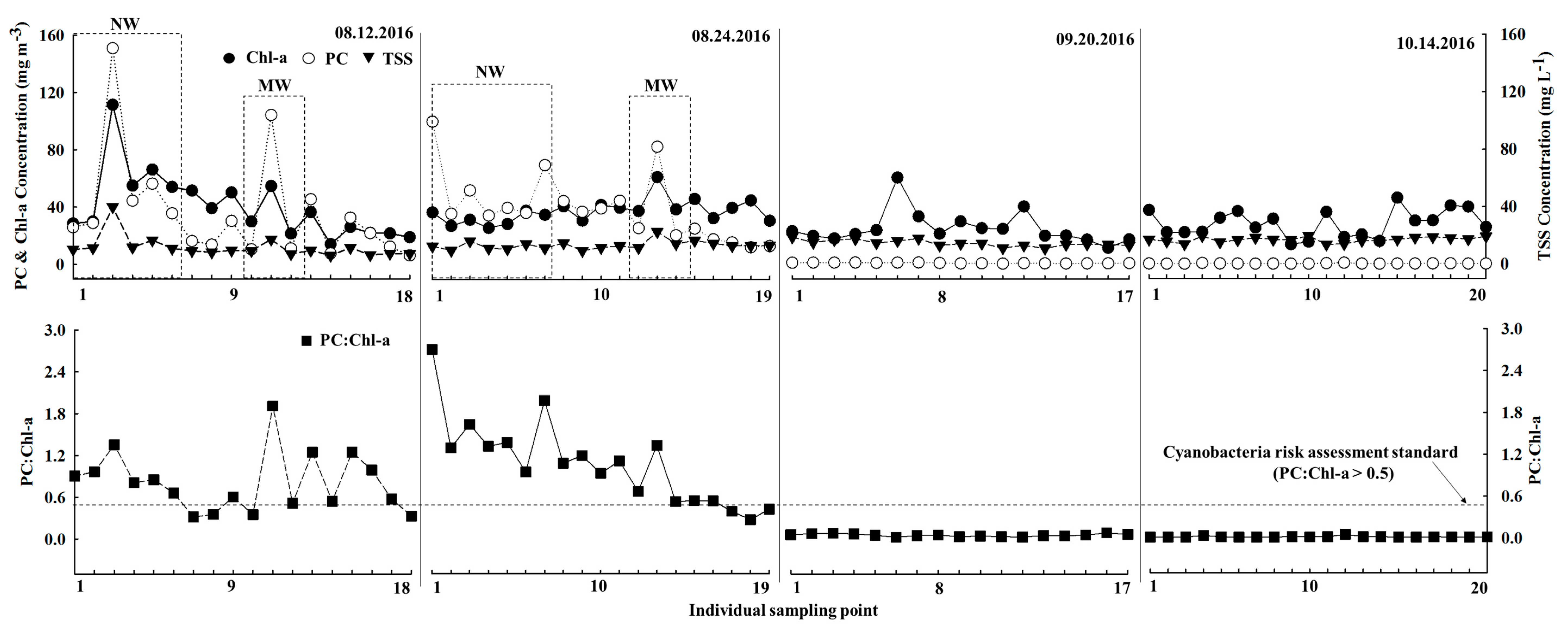
3.1. Algal Variation in the Baekje Weir

Figure 3 shows the temporal variation in PC, Chl-a, PC:Chl-a values, and TSS during the sampling period. The measured PC and Chl-a ranged from 0.19 to 150.90 mg m−3 and from 11.85 to 111.40 mg m−3, respectively (Table 1). Thus, the PC:Chl-a value ranged from 0.0062 to 2.72. The high PC concentration resulted in a high PC:Chl-a value (Figure 3). In addition, the observed concentration of TSS measured from 6.27 to 40.14 mg L−1.
On 12 and 24 August 2016, the PC, Chl-a, and TSS concentrations were relatively high compared to those of the other sampling events. On 14 September and 20 October 2016, the PC concentration was near 0, but Chl-a maintained a relatively high concentration ranging from 11.85 to 60.88 mg m−3. The TSS concentration was also maintained between 11.36 mg L−1 and 19.60 mg L−1.

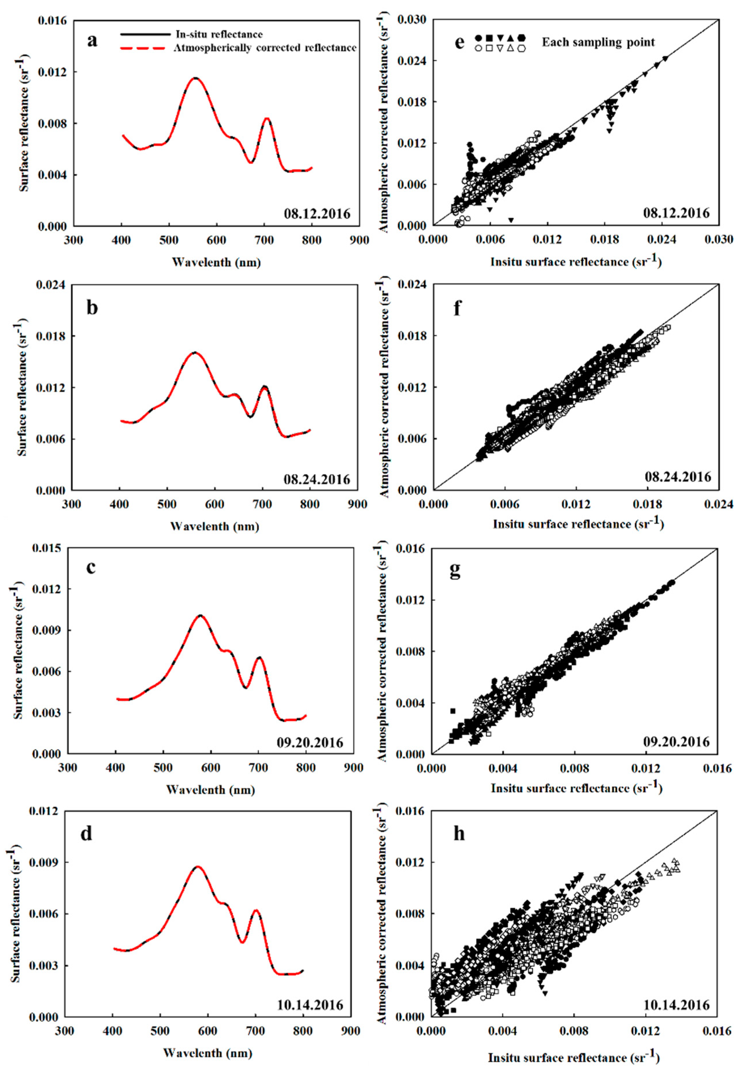
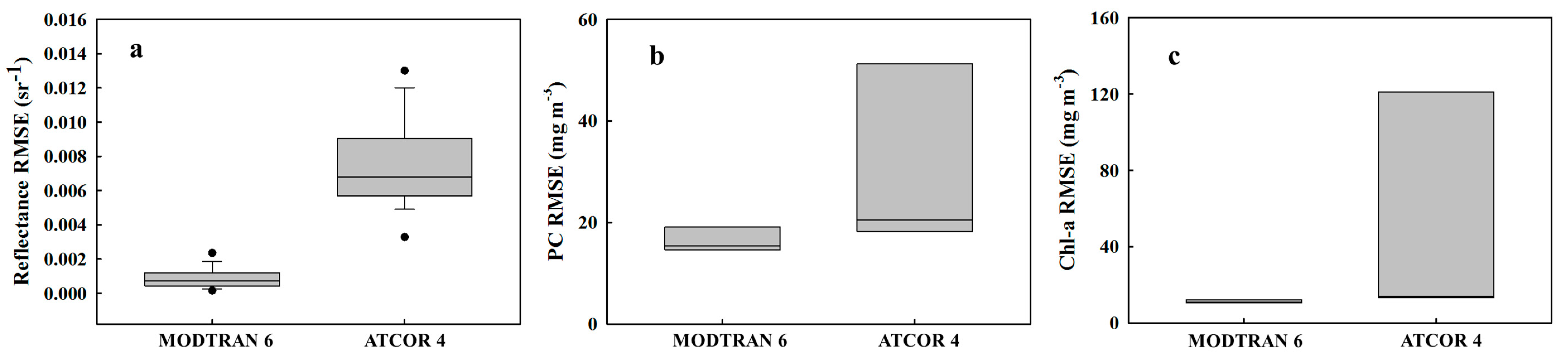
3.2. Performance of Atmospheric Correction Techniques

Figure 4 and Figure S1 show the atmospheric correction results achieved using MODTRAN 6 and ATCOR 4. The averaged spectra showed good agreement with in-situ reflectance (Figure 4a–d) while the correlation between the corrected reflectance of the individual bands and the in-situ reflectance was concentrated along the 1:1 line (Figure 4e–h). In contrast, the reflectance spectra corrected using ATCOR 4, shown in Figure S1, are four orders of magnitude smaller than the in-situ reflectance and are less correlated with the observed reflectance. The overall atmospheric correction performance of both models is presented in Table S4. Most NSE values of MODTRAN 6 were higher than 0.8. In addition, the RMSE values for the MODTRAN 6 results were smaller than 0.0034 sr−1.
All reflectance corrected by the ATCOR 4 values had negative NSE values (Table S4) while their RMSE values were higher than those of the MODTRAN 6 results. The average error of the MODTRAN 6 and ATCOR 4 reflectance across all four sampling events is shown in Figure S3. The reflectance error of MODTRAN 6 was less than 30%. However, the errors in the wavelength ranges of λ < 500 nm and λ > 700 nm were higher than the errors in the other wavelength bands (Figure S3a–d, Table 2). In particular, the corrected reflectance at 439 nm, 445 nm, 755 nm, and 779 nm had higher errors than the other bands. Similar to MODTRAN 6, the errors of ATCOR 4 increased when the wavelength was less than 500 nm and greater than 700 nm (Figure S3e–h). The error of the ATCOR 4 correction was between 99% and 100%, which was three times higher than that of the MODTRAN 6 correction results. The simulated reflectance from the ANN model is shown in Figure S2. The simulation has an NSE value of 0.79 while the error was largely between 10% and 50% (Table 2). The reflectance error of the ANN simulation was greater than that of the MODTRAN 6 simulation but was less than that of the ATCOR 4. In addition, all three different methods did not show good performance for the imagery taken on 14 October 2016.

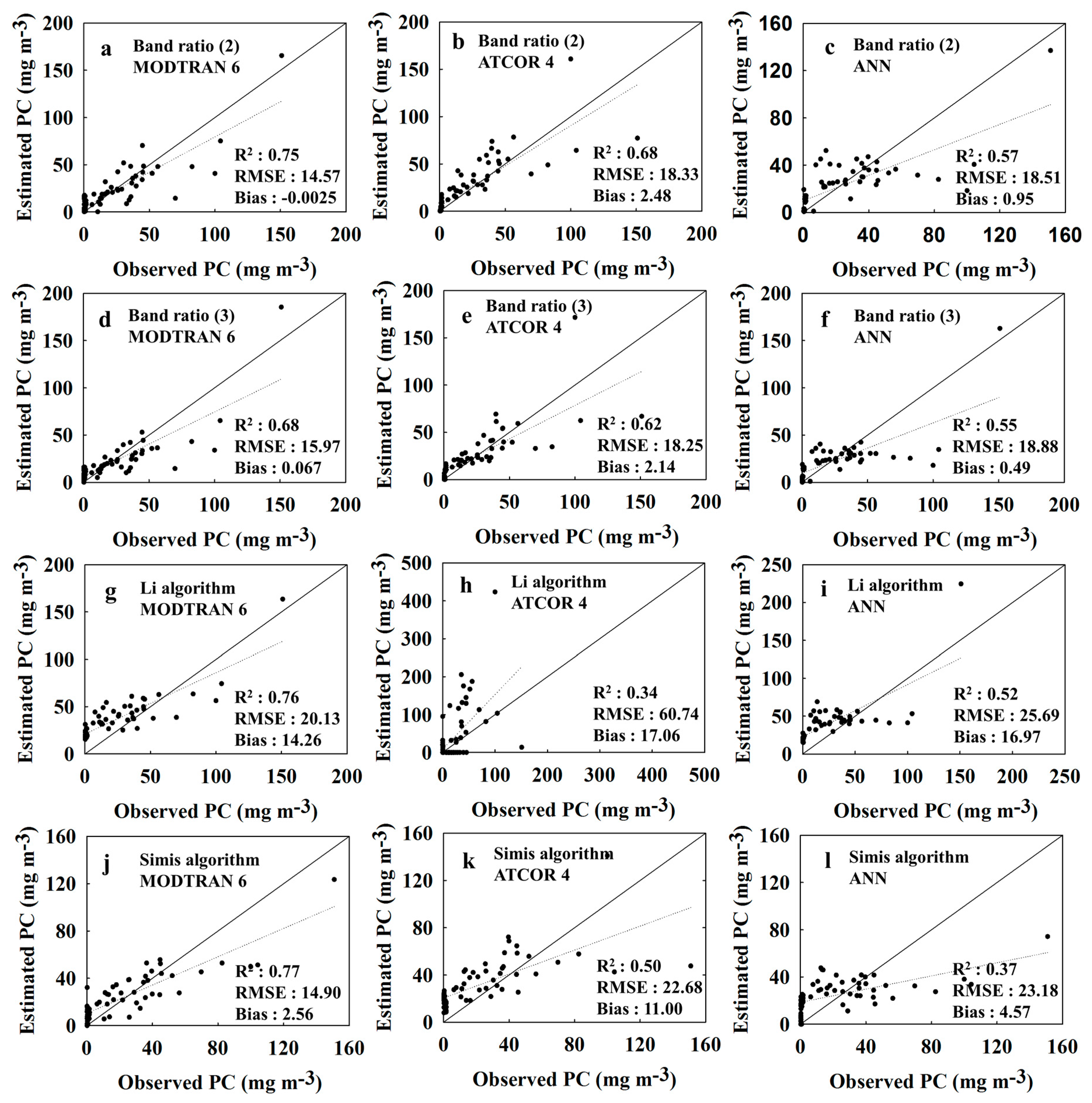
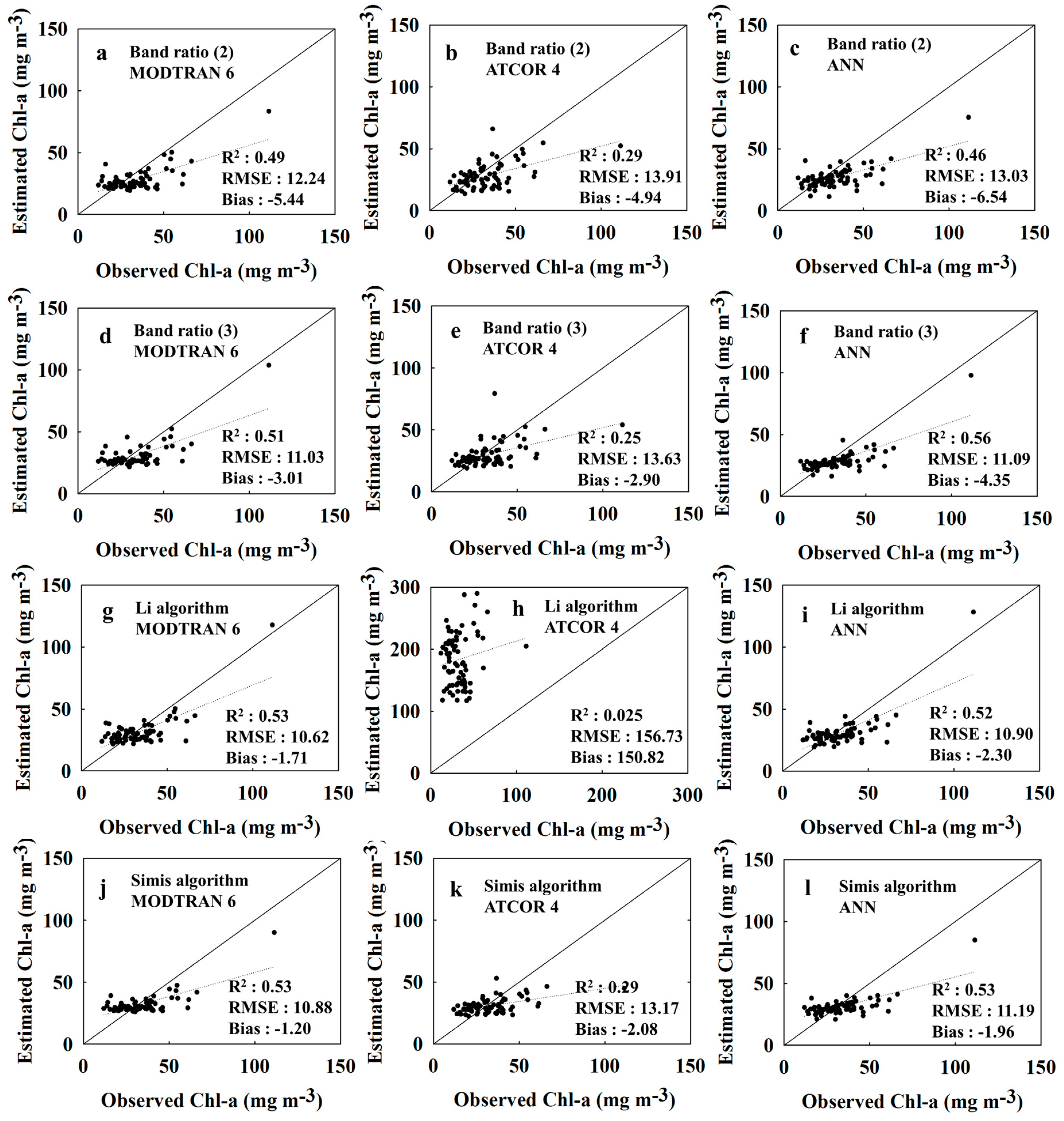
3.3. Performance of the Bio-Optical Algorithm

Figure 5 and Figure 6 show the results of the bio-optical algorithm for estimating PC and Chl-a, respectively. Figures S4 and S5 show the performance of the absorption coefficient with respect to PC and Chl-a estimation, respectively. Multi-objective optimization of the IOP algorithm was conducted using the observed reflectance data. The optimized parameters were applied to build the IOP algorithm using the reflectance data that had been atmospherically corrected using MODTRAN 6, ATCOR 4, or the ANN simulation (Table 3). The reflectance corrected by MODTRAN 6 showed good agreement with the observed PC concentration with R2 values ranging from 0.68 to 0.77. The R2 values of the Chl-a algorithms ranged from 0.49 to 0.53.
The PC and Chl-a algorithm results from ATCOR 4 showed a lower accuracy than MODTRAN 6-based results in terms of R2 and RMSE (second column in Figure 5 and Figure 6). Based on the ANN simulation (fourth column in Figure 5 and Figure 6), the R2 values of the PC and Chl-a algorithms ranged from 0.37 to 0.57 and 0.46 to 0.56, respectively.
Among the PC algorithms, the Simis algorithm with MODTRAN 6 correction showed the highest accuracy with an R2 value of 0.77, an RMSE of 14.90 mg m−3, and a bias of 2.56 mg m−3 (Figure 5j). This resulted from a good agreement of the estimated absorption coefficient with the observed coefficient (Figure S4a). For Chl-a estimation, the Simis algorithm with MODTRAN correction showed the highest performance with an R2 value of 0.53, an RMSE of 10.88 mg m−3, and a bias of −1.20 mg m−3 (Figure 6g). This proved the accurate estimation of the absorption coefficient (Figure S5d). Both the Li and Simis algorithms overestimated the PC and Chl-a concentrations when both concentrations were below 25 mg m−3 (third and fourth row in Figure 5 and Figure 6). Under atmospheric correction by ATCOR 4, the Li algorithm was not responsive to PC and Chl-a concentration. This resulted in the lowest R2 values of 0.34 and 0.025 and the highest RMSE values of 60.74 mg m−3 and 156.73 mg m−3, as well as the highest biases of 17.06 mg m−3 and 150.82 mg m−3, respectively.

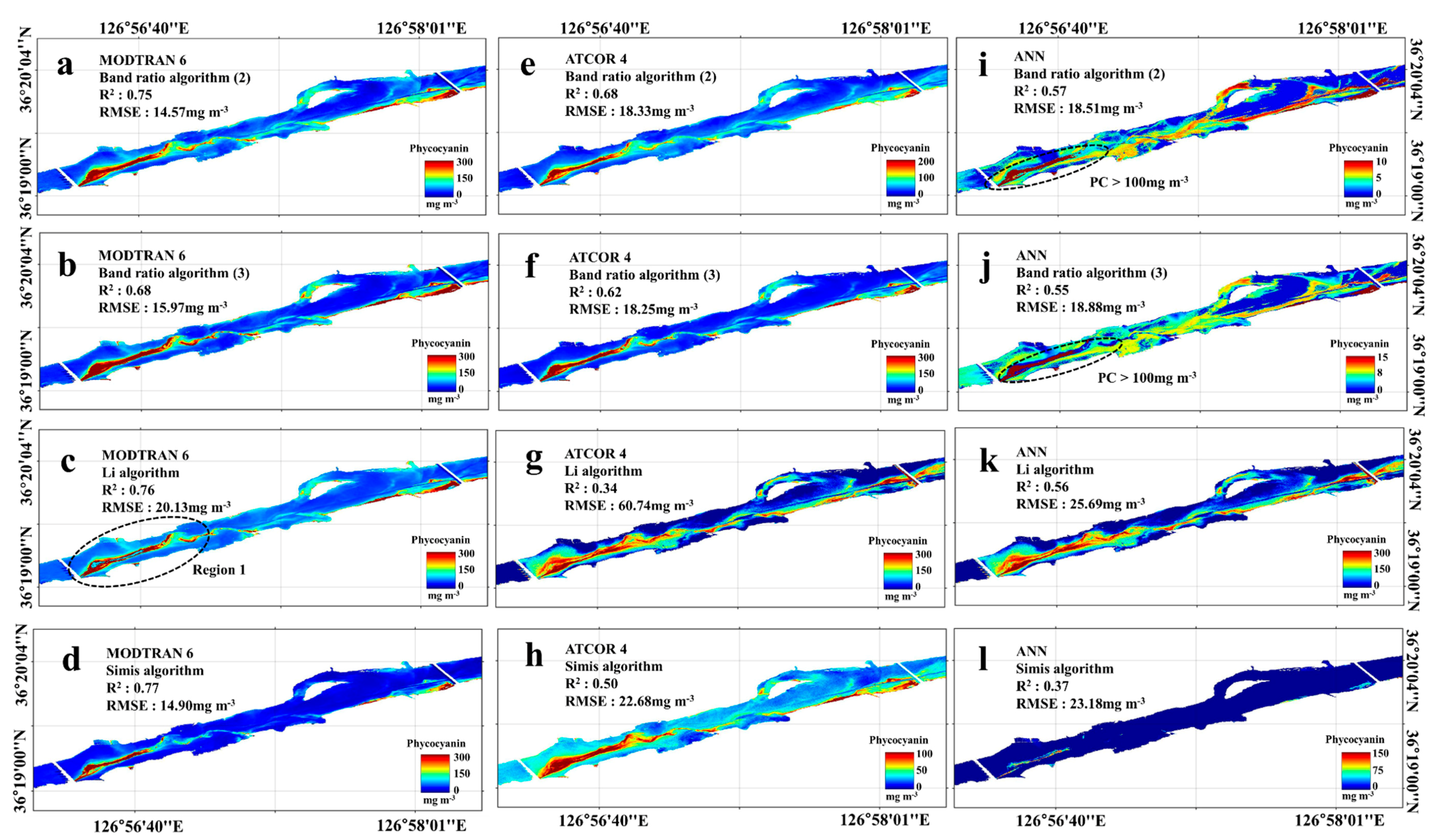
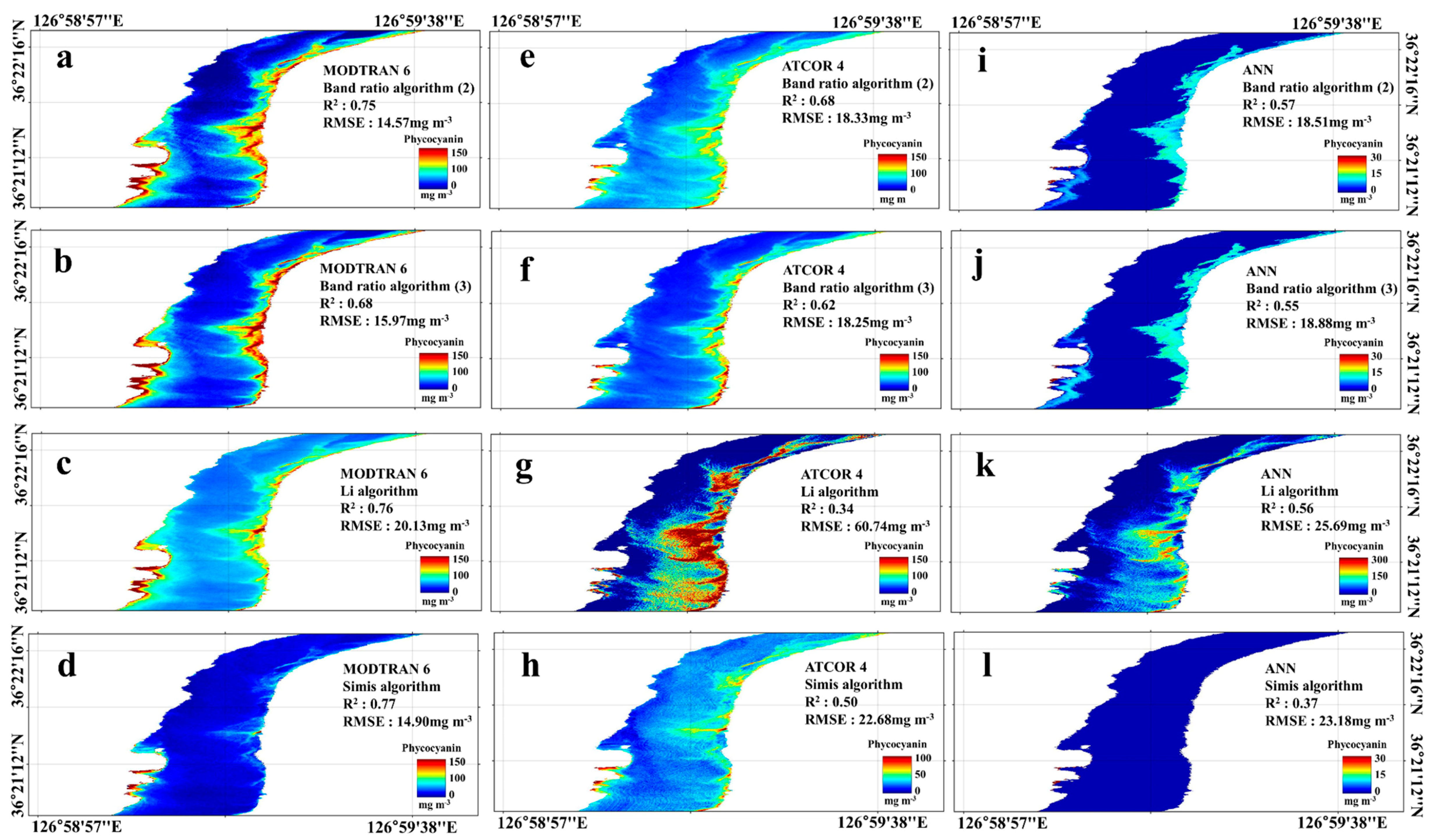
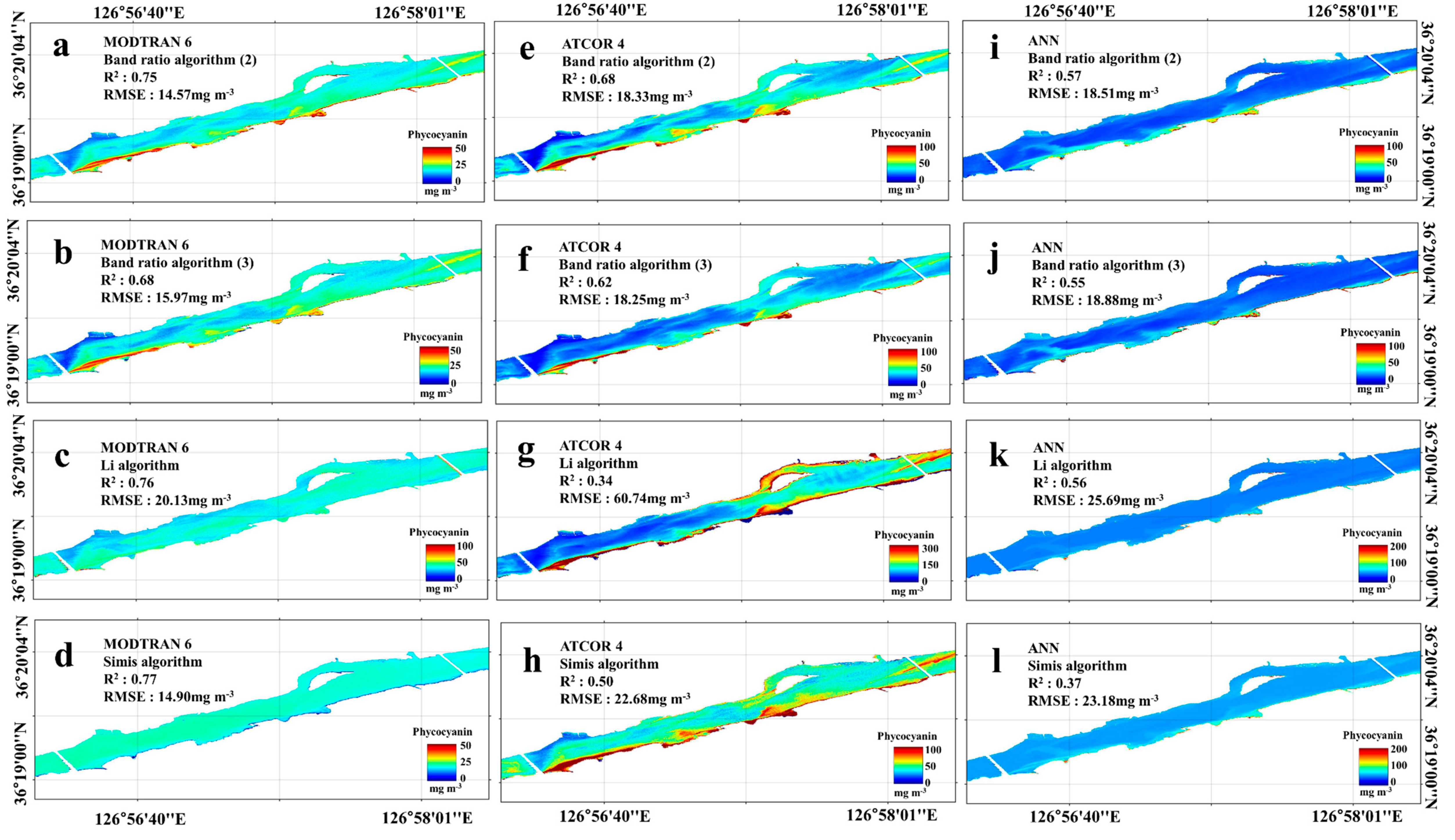
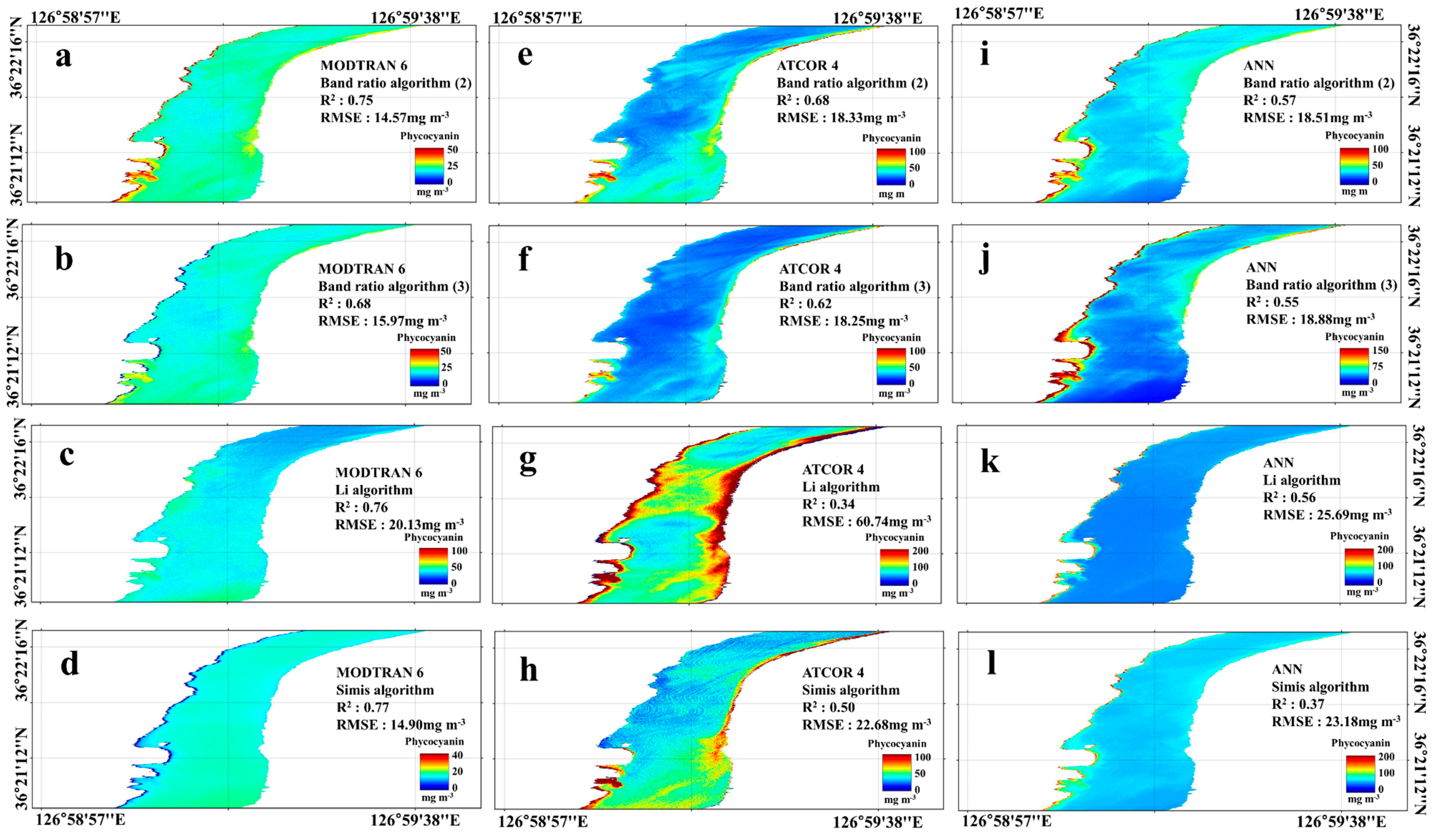
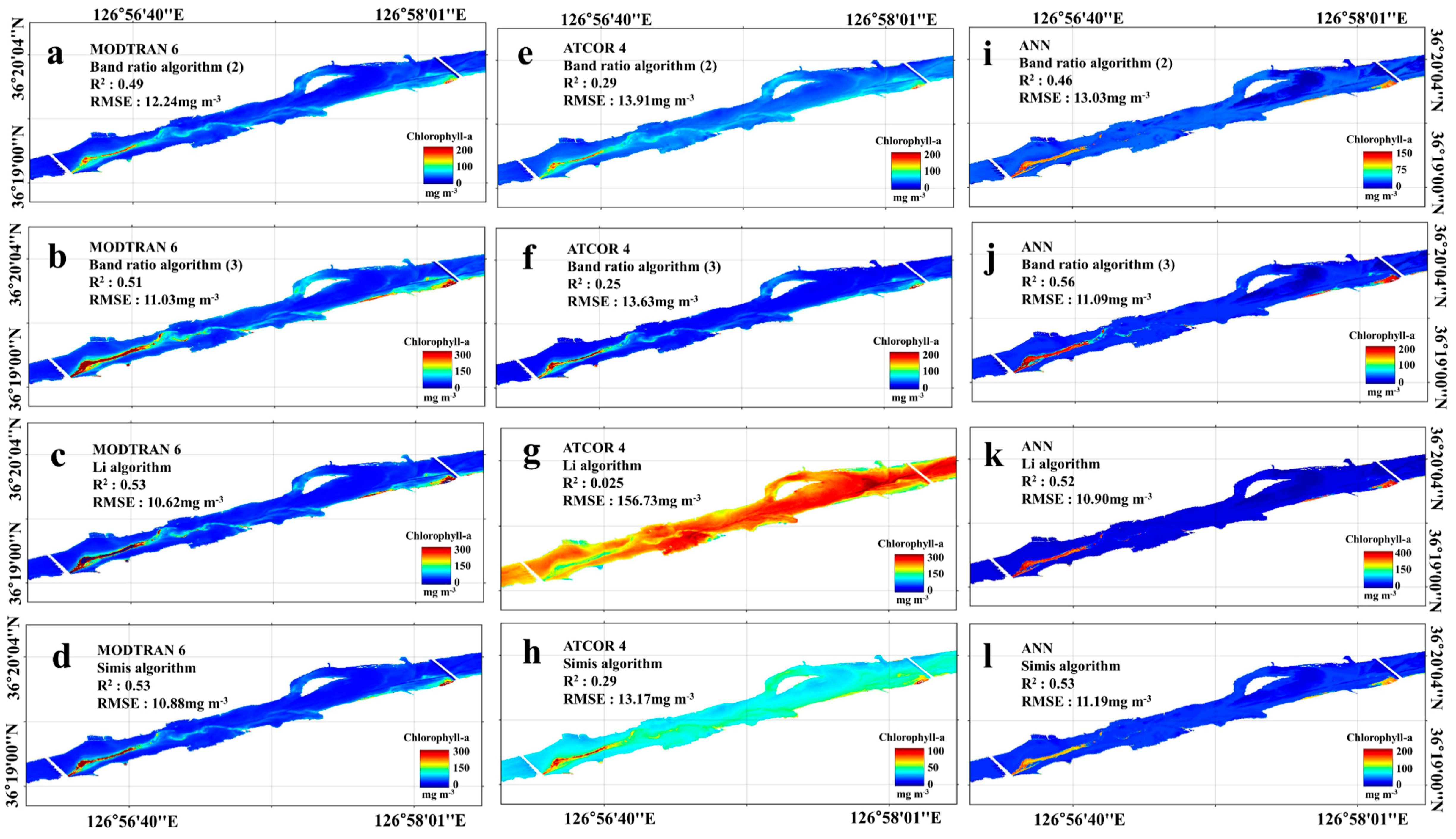
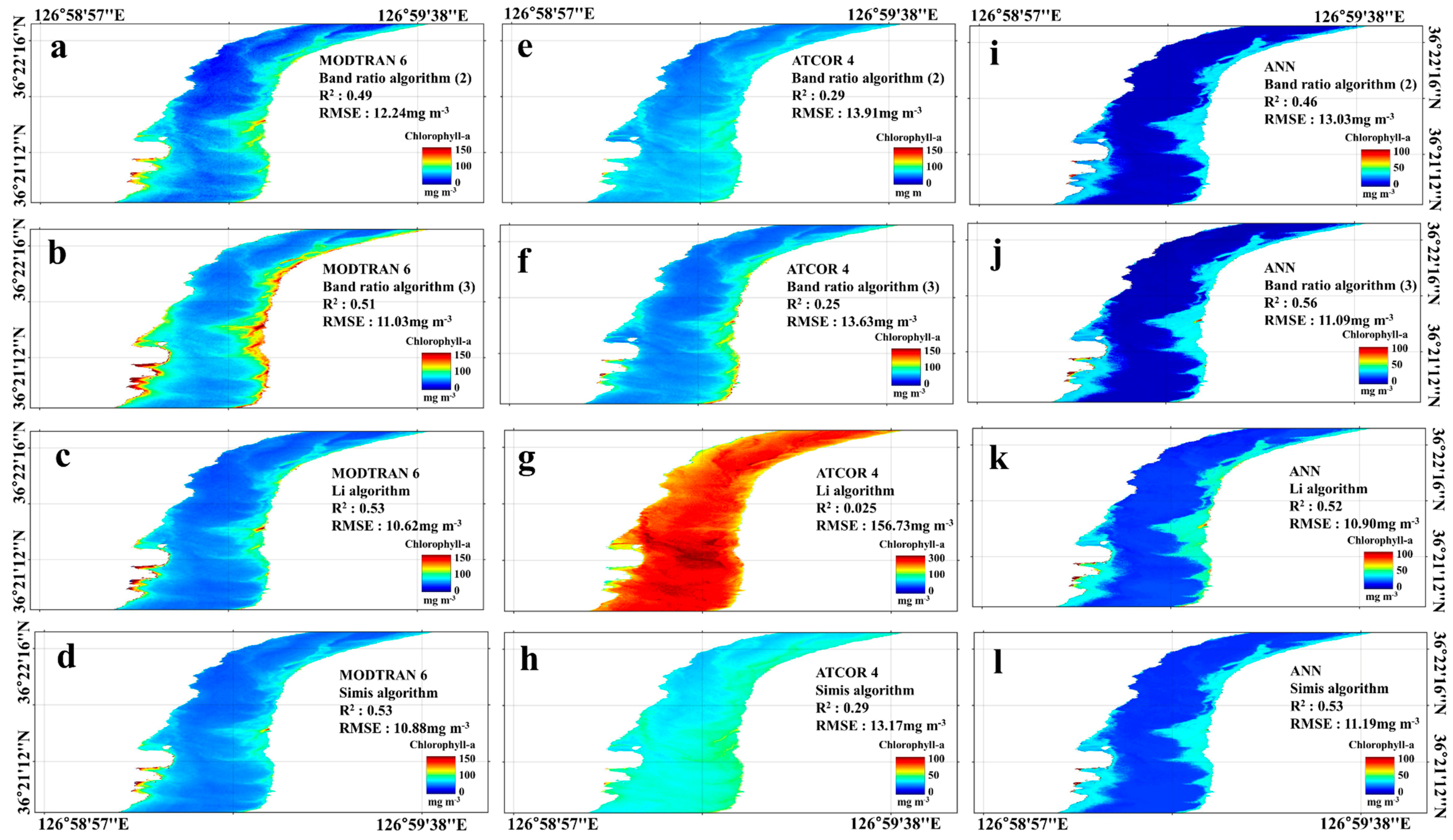
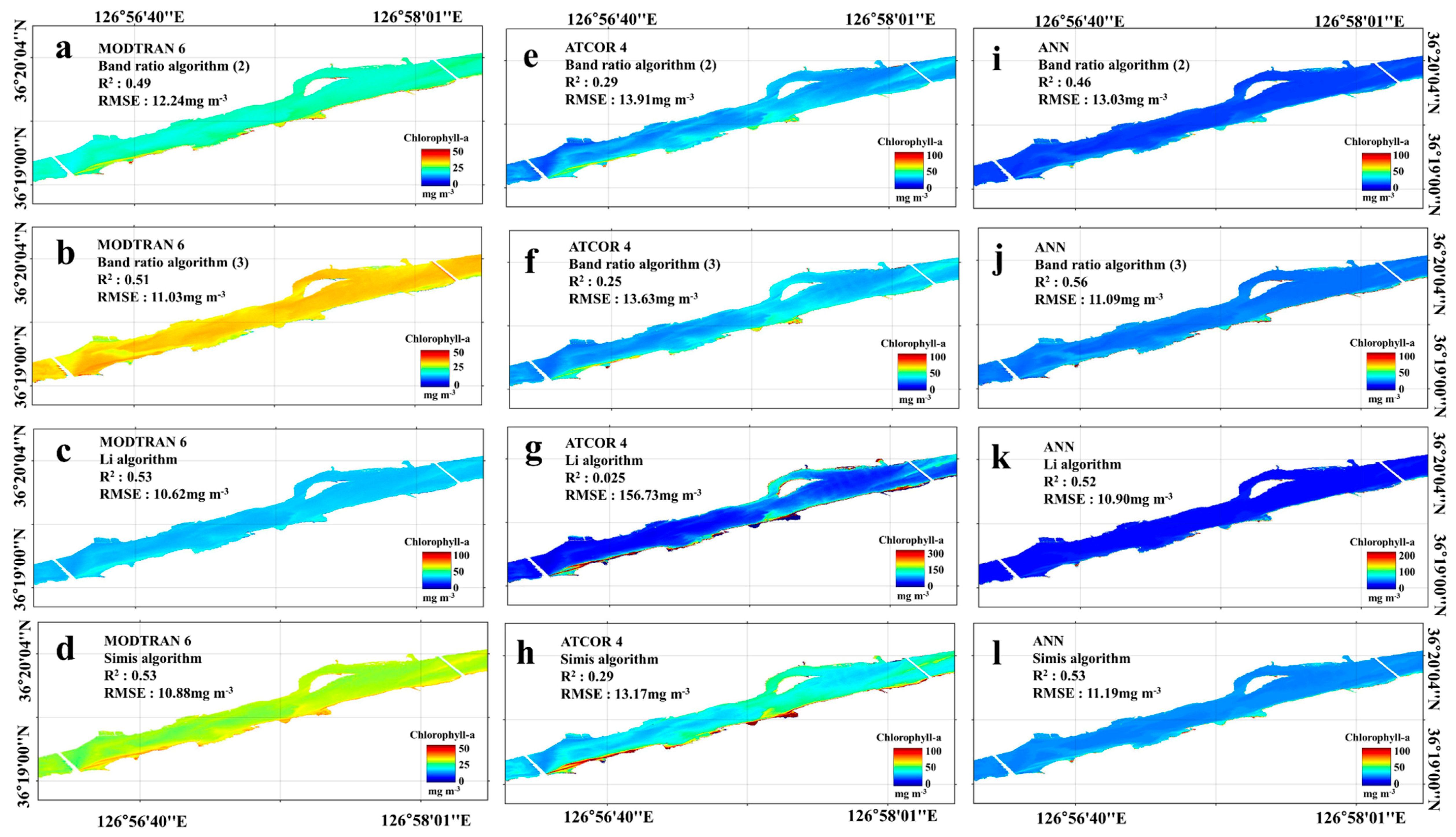
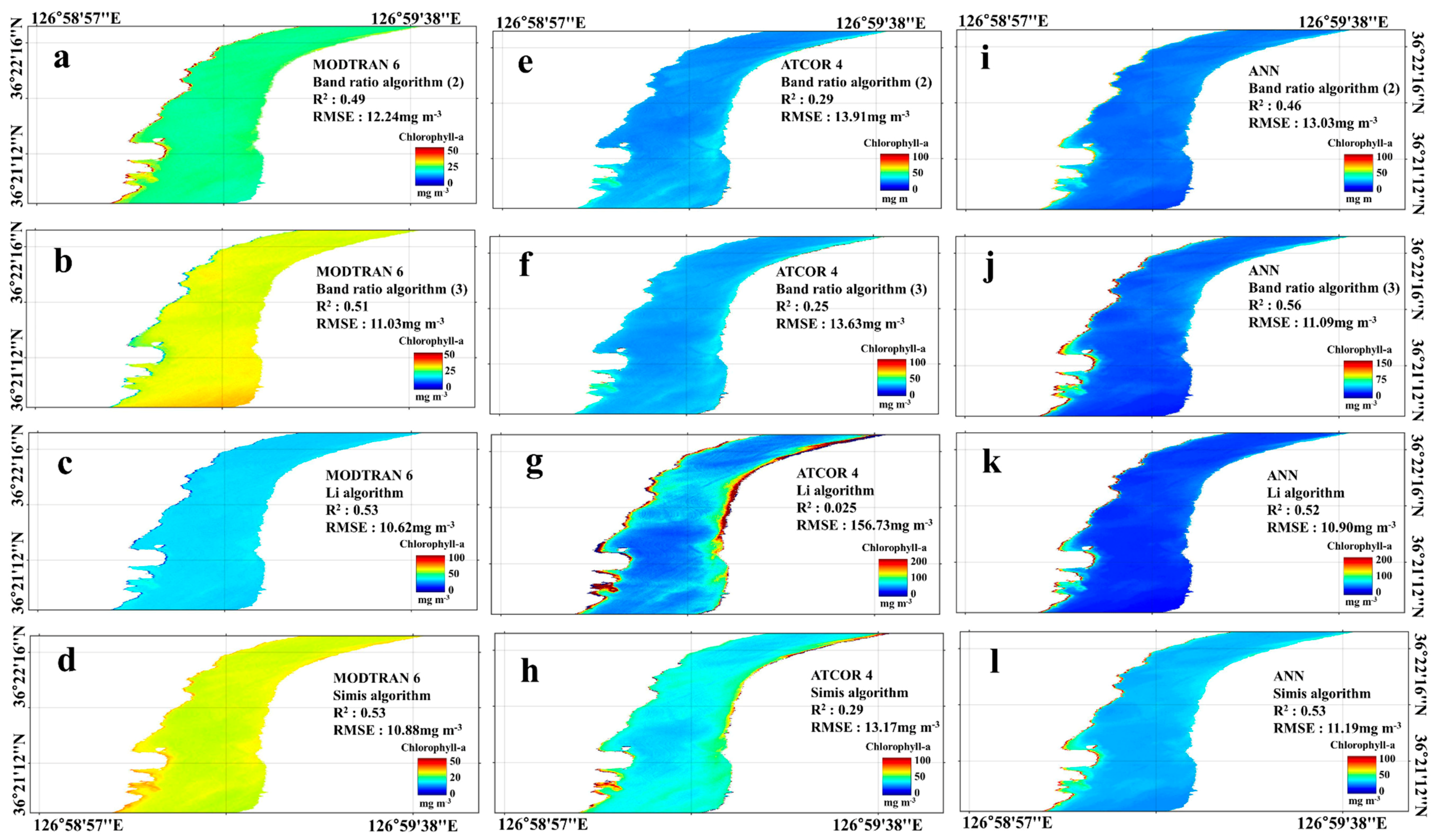
3.4. PC and Chl-a Distribution Map

Following MODTRAN 6, ATCOR 4, and ANN correction, the spatial distribution of PC and Chl-a showed a similar pattern (Figure 7, Figure 8, Figure 9, Figure 10, Figure 11, Figure 12, Figure 13 and Figure 14). However, the PC and Chl-a concentration obtained from the reflectance data corrected using MODTRAN 6 was relatively high compared to the concentration obtained from reflectance data corrected using ATCOR 4 and ANN. A distinctive spatial distribution of high PC and Chl-a concentration was observed in Section 1 on 12 August 2016. In addition, a high PC and Chl-a concentration level was distributed along the left edge of the river on 12 and 24 August 2016.
The IOP algorithms showed higher concentrations of PC and Chl-a than those of the AOP algorithm in terms of MODTRAN 6, ATCOR 4, and ANN correction. However, the Simis algorithm with ANN correction did not correctly estimate the PC distribution (Figures 7k and 8k). The PC concentrations of the Li algorithm with MODTRAN 6 correction were underestimated in the area highlighted by the dotted circle (i.e., region 1 in Figure 7c); however, the Li algorithm with ATCOR 4 correction showed the opposite Chl-a concentration pattern compared to the other results (Figures 11g and 12g). On the other sampling dates (20 September and 14 October 2016), the PC and Chl-a concentrations and spatial distribution were fairly constant (Figures S6–S13). The band ratio (2) algorithm produced a reasonable concentration range of spatial distributions for PC during these sampling events. In contrast, the IOP algorithms using reflectance data corrected by MODTRAN 6, ATCOR 4, and ANN showed higher PC and Chl-a concentrations than those of the AOP algorithms. Most algorithms showed concentrations ranging from 10 to 40 mg m−3 for the Chl-a estimations.

4. Discussion

4.1. Variation in Algae in the Baekje Reservoir

The HSI images taken on 12 and 24 August 2016 succinctly identified a cyanobacteria-dominant bloom in the reservoir. Most of the PC:Chl-a values on 12 and 24 August 2016 were observed to be greater than 0.5, which is a standard for assessing whether the cyanobacteria bloom is at risk. In particular, the PC:Chl-a of 12 and 24 August 2016 could be classified as medium risk because of the relatively high Chl-a concentrations [60].
The low PC concentration and relatively high Chl-a concentration on 20 September and 14 October 2016 signified an algal species succession from cyanobacteria to diatoms and green algae. This occurrence was mainly because of the observed water temperature between 18 °C and 22 °C, which is not a preferred growth condition for cyanobacteria [9]. The total number of cyanobacteria cells significantly decreased from 105,840 cells mL−1 to 23,840 cells mL−1 on 20 September and 14 October 2016, respectively, while the total cells of green algae and diatoms did not change substantially: 116,512 cells mL−1 (i.e., 30% green algae and 70% diatoms) on 20 September and 110,816 cells mL−1 (i.e., 30% green algae and 70% diatoms) on 14 October 2016.

4.2. Atmospheric Correction Performance

Overall, the atmospheric correction performance of MODTRAN 6 was acceptable, with an NSE value greater than 0.80. Although the averaged reflectance spectra of the MODTRAN 6 atmospheric correction was in good agreement with the in-situ spectra, the corrected reflectance result had 20–30% error in the blue and green bands (i.e., λ < 500 nm) and the near infrared bands (i.e., λ > 700 nm) (Figure S3). In addition to the uncertainty of the in-situ measurement, the reflectance errors caused by atmospheric correction have been documented by several authors. Bernstein et al. [52] reported that reflectance corrected using MODTRAN differed from the observations because of the lack of in-situ reflectance data as well as difficulties in the elimination of absorption and scattering properties in the atmospheric correction. Gao et al. [53] emphasized that retrieval of aerosol information allowed description of the absorption and scattering properties, which could be used to reduce the reflectance error in wavelength regions where λ < 500 nm and λ > 700 nm. Adler-Golden et al. [74] highlighted that the poor performance of the atmospheric correction method was driven by the high water column which increased the fractional error of the reflectance bands because of the combined effects of atmospheric absorption and scattering. Hunter et al. [33] noted that intensive scattering of aerosol and water vapor resulted in poor correction performance in the wavelength regions of λ < 500 nm and λ > 750 nm.
Similarly, the atmospheric correction performance of ATCOR 4 in this study may have been affected by the limited available data on the atmospheric conditions during the measurement campaigns. Hadjimitsis et al. [75] insisted that given sufficient data on the atmospheric conditions at the time of measurement, molecular absorption and scattering in the atmosphere could be described, resulting in accurate atmospheric correction using a physically based model such as ATCOR. In this study, the inaccuracy of the MODTRAN 6 atmospheric correction in certain reflectance bands and the poor performance of ATCOR 4 may have been caused by the lack of available data on important atmospheric conditions such as water vapor column and aerosol optical depth, as L path and S depend on the water vapor column, which might not have been well defined in this study (see Appendix A in the Supplementary Material). Uncertainty in the atmospheric parameters would have led to uncertainty being distributed throughout the image [22]. Another possible cause of the correction error was suggested by Matthews et al. [22], who insisted that the absence of Lambertian bidirectional reflectance distribution functions could negatively affect the accuracy of the corrected reflectance.
In addition, imperfect time-matching between ground-based and airborne monitoring may have caused distortion of the corrected reflectance because of changes in water vapor over time [33]. The outliers of the corrected reflectance were observed on 12 August 2016, because of the phytoplankton influence on the in-situ reflectance. When the massive phytoplankton occurred on the water surface, the reflectance spectra had higher values greater than 700 nm because of the increased scattering of the phytoplankton and lower values less than 500 nm because of the increased absorption of the phytoplankton [76]. Then, averaged atmospheric parameters might not consider this abnormal circumstance to estimate the surface reflectance. The corrected reflectance on 14 October 2016 was less concentrated along the 1:1 line than the reflectance results of the other sampling periods. A haze effect on the water surface might be a cause of the uncertainty of the in-situ reflectance measurement [77,78]. This might increase the scattering, which results in distorted measurement of in-situ reflectance.
The atmospheric correction using the ANN model in this study showed satisfactory performance during both the training and validation steps, which had NSE values of 0.80 and 0.76, respectively. Compared to previous studies, the authors of [51] applied an ANN to the atmospheric correction of Medium Resolution Imaging Spectrometer (MERIS) imagery to retrieve remote-sensing reflectance under the water conditions in case 2. Their model showed a high correlation between the in-situ and corrected reflectance. Schroeder et al. [50] atmospherically corrected a MERIS image in the water in case 1 that had a low RMSE value for the at-sensor radiance by using top-of-atmosphere radiance, humidity, and angle data. Goyens et al. [49] corrected atmospheric effects in a MODIS-Aqua image using an ANN model which achieved an R2 value greater than 0.8.

4.3. Bio-Optical Algorithm Application

The MODTRAN 6 correction led to the higher performance of the AOP and IOP algorithms compared to that of the ATCOR 4 correction in both PC and Chl-a estimation (Figure 15 and Figure S14). However, the AOP algorithm with ATCOR 4 correction resulted in an acceptable estimation (Figure 5b,e) as it can compensate for magnitude differences by using simple ratios [79]. The low performance of the ANN simulation might have been because of an insufficient number of reflectance input data points. Goyens et al. [49] and Schroeder et al. [51] used over 10,000 and 30,000 data points, respectively, to construct an ANN model. They showed an acceptable correction accuracy with R2 and RMSE values of 0.8 and ± 1.1 W m−2 μ m−1 sr−1, respectively. The IOP algorithms were directly influenced by the correction performance, because these algorithms directly use the corrected reflectance in various wavelength bands. This could be caused by monitoring uncertainty in remote-sensing reflectance data [30,80]. Thus, the IOP algorithms were more significantly affected by the performance of the atmospheric correction than the AOP algorithms because of the intervention of the various reflectance bands (Figure S14). IOP algorithms commonly overestimate low PC concentrations because of the difficulty in accurately measuring the optical intensity at low PC concentrations. Li et al. [30] found degraded performance for the Li and Simis algorithms in low PC conditions because of optical interference, for example, from colored dissolved organic matter.
Although Li et al. [30] improved the algorithmic results at low PC concentrations by considering the interference effect in the algorithm, the Li algorithm still overestimated the PC concentration under those conditions. This implies that, in the case of IOP algorithms, it might be difficult to correctly estimate lower PC concentrations using the combination of various reflectance bands. Thus, AOP algorithms would be a straightforward means to describe low PC concentrations and their spatial distribution.
Even though Chl-a estimates showed lower precision than those of the PC estimates, the MODTRAN 6 correction showed more accurate results of the bio-optical algorithms than those using reflectance data corrected by ATCOR 4 and ANN (first column in Figure 6). The poor performance of the Chl-a algorithms was mainly from the relatively low level of Chl-a concentrations on 20 September and 14 October 2016. During these sampling events, the influence of interference such as TSSs might have increased as the TSS concentration was maintained from 12 mg L−1 to 20 mg L−1 (Figure 3). This was proven by the nonlinear relationship between the particulate matter and Chl-a as suggested by Bricaud et al. [81], Garver et al. [82], and Yentsch and Phinney [83]. They found that as Chl-a concentration decreased, the particulate optical properties increased. The particulate interference eventually resulted in poor performance of the Chl-a algorithms.

4.4. Spatial Distribution Map of Algal Concentration

Under the MODTRAN 6 correction, the Li algorithm was able to describe the spatial distribution of PC appropriately on 12 August 2016. However, it still underestimated the PC concentration in the middle of region 1 because of the unstably corrected reflectance in bands greater than 700 nm (Figure 7c). In addition, the Chl-a distribution of the Li algorithm showed reverse concentration pattern because low reflectance values greater than 700 nm decreased b ( λ w ) , which resulted in an abnormally high Chl-a estimation (Equation (9)).
In the middle of the river in Section 1 on 12 August (Figure 7 and Figure 11), the gate operation for the hydropower plant caused a tailed shape of the PC and Chl-a distribution [9]. In this near-Baekje Weir region, high concentrations of PC and Chl-a were observed. This resulted in a high PC:Chl-a value, which resulted in a caution index for the cyanobacteria dominant bloom (first row in Figure S15). Likewise, the PC:Chl-a value on 24 August 2016 was high near the Baekje Weir region (second row in Figure S15). Thus, this near-Baekje Weir region could be classified as a medium risk zone on 12 and 24 August 2016 [33,60]. PC concentrations tended to be high along the edge of the river because the water flow was slower there than in the middle of the river, leading to longer water retention times. Figure 16 shows the negative relationship between flow velocity and PC:Chl-a on 12 and 24 August 2016 (p-value = 0.003). This proved that the cyanobacteria favor a long water retention time to form a dominant cyanobacteria bloom. Previous studies are in agreement with cyanobacteria blooms occurring when the water retention time is long [10,84,85,86]. Further, Park et al. [9] reported that a flow velocity less than 0.06 m s−1 was a suitable physical condition for cyanobacteria growth. In addition, a high water temperature and stable nutrient concentration were proven as dominant environmental factors for PC distribution on 12 and 24 August 2016 [9]. Overall, atmospheric correction using the ANN simulation resulted in a similar PC and Chl-a distribution as that using MODTRAN 6 or ATCOR 4. Sufficient input datasets are required to obtain a reasonable performance using the ANN model. If there is not sufficient input data, the results are often observed to have a single simulation value with various observed values on the dotted line as shown in Figure S2 [87]. Therefore, it is assumed that the scarcity of the input data for the ANN simulation resulted in relatively poor performance in developing the PC and Chl-a concentration map.

5. Conclusions

This study estimated the spatial distribution of PC and Chl-a concentrations using hyperspectral image data and identified how the performance of bio-optical algorithms depended on which atmospheric correction method was used. In addition, how the algae were distributed by influence factors such as flow velocity was also analyzed. The atmospheric correction methods investigated in this study were MODTRAN 6, ATCOR 4, and ANN. Field monitoring and experimental analysis were conducted, after which, bio-optical algorithms were built to quantify PC and Chl-a concentrations using hyperspectral image data. IOP algorithms were optimized using multi-objective optimization. MODTRAN 6, ATCOR 4, and ANN all succeeded in correcting for atmospheric effects on the hyperspectral image obtained from airborne monitoring. Both AOP and IOP algorithms generated maps of the spatial distribution of PC and Chl-a concentrations using the corrected images. The major findings of this study are as follows:
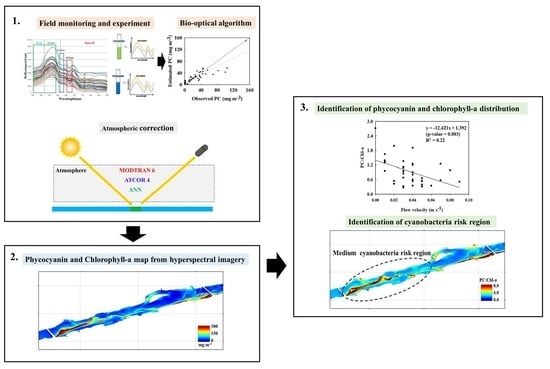
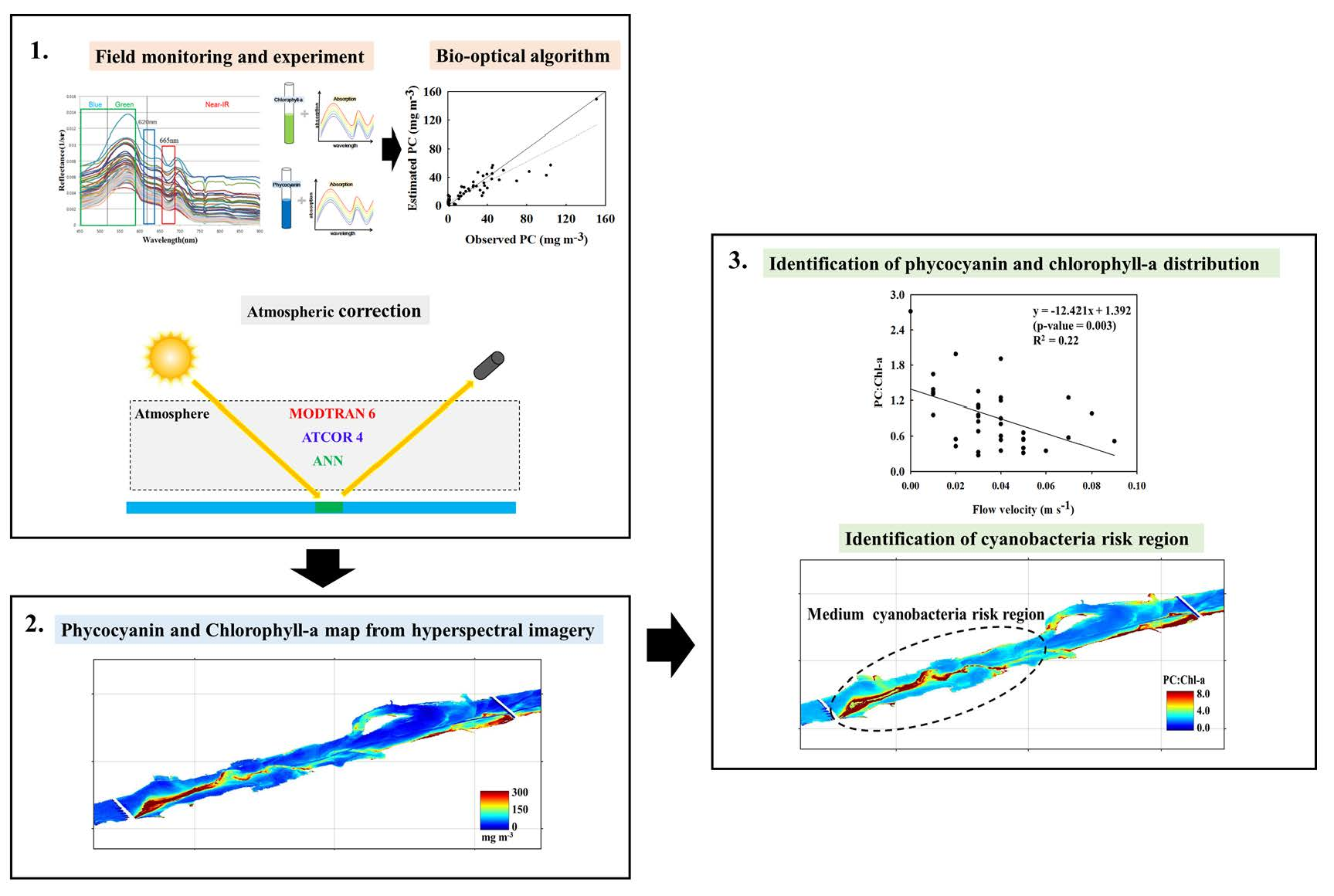
  • The cyanobacteria bloom on 12 and 24 August 2016 occurred as the PC:Chl-a value was greater than 0.5. A succession of algal species from cyanobacteria to diatoms was then observed on 20 September and 14 October 2016.
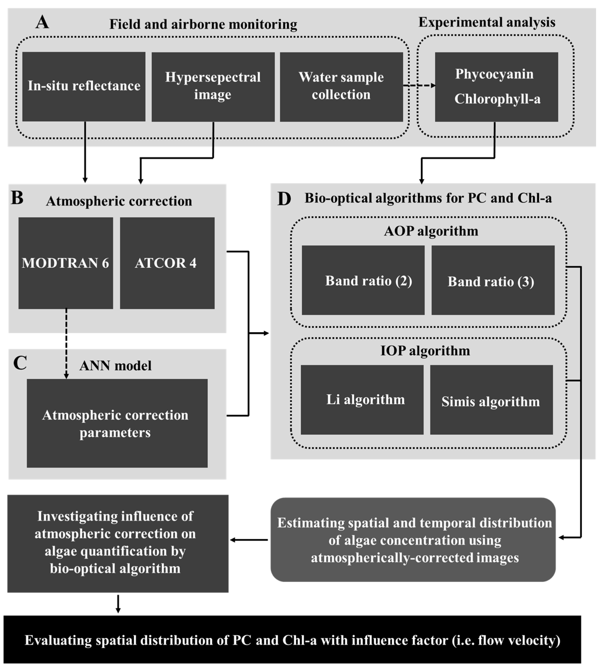
  • MODTRAN 6 provided reasonable atmospheric correction performance compared to that of ATCOR 4. However, the accuracy was low in certain regions of the reflectance spectra ( λ < 500 nm and λ > 700 nm). This was mainly because of insufficient atmospheric observations during the campaigns.
  • The most accurate atmospheric correction by MODTRAN 6, compared to ATCOR 4 and ANN, contributed to improving the performance of the bio-optical algorithms in terms of the estimation of PC and Chl-a concentration. The ANN model was found to require large quantities of input data to achieve accurate simulation results.
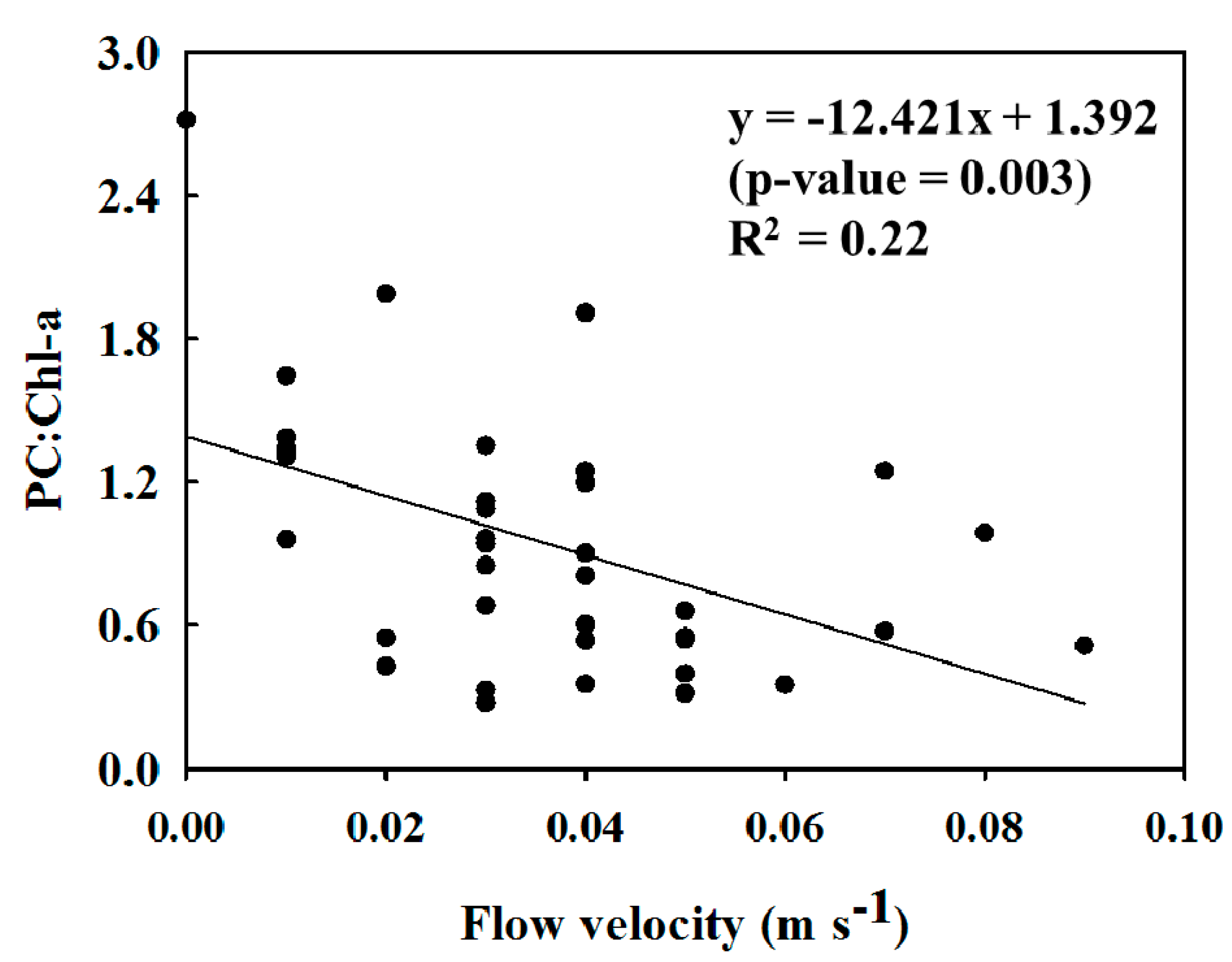
  • The spatial distribution of a high PC:Chl-a value was derived using the flow velocity of less than 0.06 m s−1. This study directly proved that the influence factor of the dominant PC bloom was a long water retention time.
This study identified the effect of the atmospheric correction method used in HSI on PC and Chl-a concentrations derived from images, and it evaluated the influence factor on the algal distribution. Thus, atmospheric correction performance has been shown to be critical in providing useful, informative, and precise maps of the spatial distribution of PC when employing airborne or satellite imagery.

Supplementary Materials

The following are available online at https://www.mdpi.com/2072-4292/10/8/1180/s1, Appendix A: Atmospheric correction of ATCOR 4, MODTRAN 6, and ANN, Table S1: MODTRAN input composition, Table S2: Solar angle for geometry specific input, Table S3: Input information for the ANN, Table S4. Atmospheric correction performances of MODTRAN 6 and ATCOR 4, Figure S1: Atmospheric correction results using ATCOR 4. Panels a–d show the average in-situ and corrected surface reflectance ρ surf . Panels e–h show the correlation between the observed and corrected results at different wavelength for each sampling point, Figure S2: ANN simulation atmospheric correction results for overall wavelengths, Figure S3: Reflectance error (%) of the atmospheric correction. Panels a-d show the MODTRAN 6 correction error and panels e-h show the ATCOR 4 correction error, Figure S4: Optimized absorption coefficient results of PC algorithm with respect to in-situ and atmospheric corrected reflectance. Panels a–d show Li algorithm results. Panels d–f show Simis algorithm results. abs indicates absorption coefficient at 622 nm, Figure S5: Optimized absorption coefficient results of Chl-a algorithm with respect to in-situ and atmospheric corrected reflectance. Panels a-d show Li algorithm results. Panels d-f show Simis algorithm results. abs indicates absorption coefficient at 660 nm, Figure S6: Phycocyanin concentration images 20 September 2016 in Section 1. Panels a–d show the PC distribution driven by the MODTRAN 6 atmospheric correction. Panels e–h show the PC distribution driven by the ATCOR 4 atmospheric correction. Panels i–l show the PC distribution driven by the ANN atmospheric correction, Figure S7: Phycocyanin concentration images on 20 September 2016 in Section 2. Panels a–d show the PC distribution driven by the MODTRAN 6 atmospheric correction. Panels e–h show the PC distribution driven by the ATCOR 4 atmospheric correction. Panels i–l show the PC distribution driven by the ANN atmospheric correction, Figure S8: Phycocyanin concentration images on 14 October 2016 in Section 1. Panels a–d show the PC distribution driven by the MODTRAN 6 atmospheric correction. Panels e–h show the PC distribution driven by the ATCOR 4 atmospheric correction. Panels i–l show the PC distribution driven by the ANN atmospheric correction, Figure S9: Phycocyanin concentration images on 14 October 2016 in Section 2. Panels a–d show the PC distribution driven by the MODTRAN 6 atmospheric correction. Panels e–h show the PC distribution driven by the ATCOR 4 atmospheric correction. Panels i–l show the PC distribution driven by the ANN atmospheric correction, Figure S10: Chlorophyll-a concentration images on 20 September 2016 in Section 1. Panels a–d show the Chl-a distribution driven by the MODTRAN 6 atmospheric correction. Panels e–h show the Chl-a distribution driven by the ATCOR 4 atmospheric correction. Panels i–l show the Chl-a distribution driven by the ANN atmospheric correction, Figure S11: Chlorophyll-a concentration images on 20 September 2016 in Section 2. Panels a–d show the Chl-a distribution driven by the MODTRAN 6 atmospheric correction. Panels e–h show the Chl-a distribution driven by the ATCOR 4 atmospheric correction. Panels i–l show the Chl-a distribution driven by the ANN atmospheric correction, Figure S12: Chlorophyll-a concentration images on 14 October 2016 in Section 1. Panels a–d show the Chl-a distribution driven by the MODTRAN 6 atmospheric correction. Panels e–h show the Chl-a distribution driven by the ATCOR 4 atmospheric correction. Panels i–l show the Chl-a distribution driven by the ANN atmospheric correction, Figure S13: Chlorophyll-a concentration images on 14 October 2016 in Section 2. Panels a–d show the Chl-a distribution driven by the MODTRAN 6 atmospheric correction. Panels e–h show the Chl-a distribution driven by the ATCOR 4 atmospheric correction. Panels i–l show the Chl-a distribution driven by the ANN atmospheric correction. Figure S14: Influence of atmospheric correction with MODTRAN 6 and ATCOR 4 on a: PC algorithm and b: Chl-a algorithm.* indicates the band ratio algorithm, ** indicates the Li algorithm, and *** indicates the Simis algorithm. Figure S15: PC:Chl-a map estimated by Li algorithm from reflectance data corrected by MODTRAN 6 in 12 and 24 August 2016.

Author Contributions

Conceptualization, J.C.P, K.H.C., and Y.P.; Field Data Collection and Experiment, J.C.P., M.L., Y.S.K, K.K., H.L., and T.K.; Data analysis, J.C.P; Atmospheric correction, J.C.P., S.B.C., and M.-H.A.; Writing-Original Draft Preparation, J.C.P.; Writing-Review and Editing, K.H.C, Y.P., and M.L.; Supervision, K.H.C and Y.P.

Acknowledgments

This research was supported by the ICT R&D program of MSIP/IITP. [1711070420, Space-time complex artificial intelligence blue-green algae prediction technology based on direct-readable water quality complex sensor and hyperspectral image] and in part by the Basic Core Technology Development Program for the Oceans and the Polar Regions of the National Research Foundation (NRF) funded by the Ministry of Science, ICT & Future Planning [grant number NRF-2016M1A5A1027457].

Conflicts of Interest

The authors declare no conflict of interest.

References

  1. Chiswell, R.K.; Shaw, G.R.; Eaglesham, G.; Smith, M.J.; Norris, R.L.; Seawright, A.A.; Moore, M.R. Stability of cylindrospermopsin, the toxin from the cyanobacterium, cylindrospermopsis raciborskii: Effect of ph, temperature, and sunlight on decomposition. Environ. Toxicol. Int. J. 1999, 14, 155–161. [Google Scholar] [CrossRef]
  2. Gerard, C.; Poullain, V. Variation in the response of the invasive species potamopyrgus antipodarum (smith) to natural (cyanobacterial toxin) and anthropogenic (herbicide atrazine) stressors. Environ. Pollut. 2005, 138, 28–33. [Google Scholar] [CrossRef] [PubMed]
  3. Paerl, H.W.; Hall, N.S.; Calandrino, E.S. Controlling harmful cyanobacterial blooms in a world experiencing anthropogenic and climatic-induced change. Sci. Total Environ. 2011, 409, 1739–1745. [Google Scholar] [CrossRef] [PubMed]
  4. Shurin, J.B.; Dodson, S.I. Sublethal toxic effects of cyanobacteria and nonylphenol on environmental sex determination and development in daphnia. Environ. Toxicol. Chem. 1997, 16, 1269–1276. [Google Scholar] [CrossRef]
  5. Wagner, C.; Adrian, R. Cyanobacteria dominance: Quantifying the effects of climate change. Limnol. Oceanogr. 2009, 54, 2460–2468. [Google Scholar] [CrossRef] [Green Version]
  6. Zanchett, G.; Oliveira, E.C. Cyanobacteria and cyanotoxins: From impacts on aquatic ecosystems and human health to anticarcinogenic effects. Toxins 2013, 5, 1896–1917. [Google Scholar] [CrossRef] [PubMed]
  7. Feng, T.; Wang, C.; Wang, P.; Qian, J.; Wang, X. How physiological and physical processes contribute to the phenology of cyanobacterial blooms in large shallow lakes: A new euler-lagrangian coupled model. Water Res. 2018, 140, 34–43. [Google Scholar] [CrossRef] [PubMed]
  8. Kim, D.M.; Park, H.S.; Chung, S.W. Relationship of the thermal stratification and critical flow velocity near the baekje weir in geum river. J. Korean Soc. Water Envrion. 2017, 33, 449–459. [Google Scholar]
  9. Park, Y.; Pyo, J.; Kwon, Y.S.; Cha, Y.; Lee, H.; Kang, T.; Cho, K.H. Evaluating physico-chemical influences on cyanobacterial blooms using hyperspectral images in inland water, korea. Water Res. 2017, 126, 319–328. [Google Scholar] [CrossRef] [PubMed]
  10. Romo, S.; Soria, J.; Fernandez, F.; Ouahid, Y.; Barón-Solá, Á. Water residence time and the dynamics of toxic cyanobacteria. Freshw. Biol. 2013, 58, 513–522. [Google Scholar] [CrossRef]
  11. Ju, H.; Choi, I.; Yoon, J.; Lee, J.; Lim, B.; Lee, S. Analysis of cyanobacterial growth pattern in bekjae weir during recent 3 years. Korean Soc. Water Enviorn. 2016, 2016, 562–563. [Google Scholar]
  12. Yoon, J.; Ju, H.; Yoon, H.; Lee, J.; Lee, J.; Lee, S. Effect of hydrological conditions on distribution characteristics of algal concentration in the geum river main stream. Korean Soc. Water Environ. 2015, 2015, 631–632. [Google Scholar]
  13. Cheung, M.Y.; Liang, S.; Lee, J. Toxin-producing cyanobacteria in freshwater: A review of the problems, impact on drinking water safety, and efforts for protecting public health. J. Microbiol. 2013, 51, 1–10. [Google Scholar] [CrossRef] [PubMed] [Green Version]
  14. Davies, J.-M.; Mazumder, A. Health and environmental policy issues in Canada: The role of watershed management in sustaining clean drinking water quality at surface sources. J. Environ. Manag. 2003, 68, 273–286. [Google Scholar] [CrossRef]
  15. Brando, V.E.; Dekker, A.G. Satellite hyperspectral remote sensing for estimating estuarine and coastal water quality. IEEE Trans. Geosci. Remote Sens. 2003, 41, 1378–1387. [Google Scholar] [CrossRef]
  16. Brezonik, P.; Menken, K.D.; Bauer, M. Landsat-based remote sensing of lake water quality characteristics, including chlorophyll and colored dissolved organic matter (CDOM). Lake Reserv. Manag. 2005, 21, 373–382. [Google Scholar] [CrossRef]
  17. Dekker, A.G. Detection of Optical Water Quality Parameters for Eutrophic Waters by High Resolution Remote Sensing. Ph.D. Thesis, University of Amsterdam, Amsterdam, The Netherlands, 1993. [Google Scholar]
  18. Hilton, J. Airborne remote sensing for freshwater and estuarine monitoring. Water Res. 1984, 18, 1195–1223. [Google Scholar] [CrossRef]
  19. Kallio, K.; Kutser, T.; Hannonen, T.; Koponen, S.; Pulliainen, J.; Vepsäläinen, J.; Pyhälahti, T. Retrieval of water quality from airborne imaging spectrometry of various lake types in different seasons. Sci. Total Environ. 2001, 268, 59–77. [Google Scholar] [CrossRef]
  20. Kiefer, I.; Odermatt, D.; Anneville, O.; Wüest, A.; Bouffard, D. Application of remote sensing for the optimization of in-situ sampling for monitoring of phytoplankton abundance in a large lake. Sci. Total Environ. 2015, 527, 493–506. [Google Scholar] [CrossRef] [PubMed]
  21. Kwon, Y.S.; Jang, E.; Im, J.; Baek, S.H.; Park, Y.; Cho, K.H. Developing data-driven models for quantifying cochlodinium polykrikoides using the geostationary ocean color imager (GOCI). Int. J. Remote Sens. 2018, 39, 68–83. [Google Scholar] [CrossRef]
  22. Matthews, M.W.; Bernard, S.; Winter, K. Remote sensing of cyanobacteria-dominant algal blooms and water quality parameters in zeekoevlei, a small hypertrophic lake, using meris. Remote Sens. Environ. 2010, 114, 2070–2087. [Google Scholar] [CrossRef]
  23. Page, B.P.; Kumar, A.; Mishra, D.R. A novel cross-satellite based assessment of the spatio-temporal development of a cyanobacterial harmful algal bloom. Int. J. Appl. Earth Obs. Geoinf. 2018, 66, 69–81. [Google Scholar] [CrossRef]
  24. Ritchie, J.C.; Zimba, P.V.; Everitt, J.H. Remote sensing techniques to assess water quality. Photogramm. Eng. Remote Sens. 2003, 69, 695–704. [Google Scholar] [CrossRef]
  25. Song, K.; Li, L.; Tedesco, L.P.; Li, S.; Hall, B.E.; Du, J. Remote quantification of phycocyanin in potable water sources through an adaptive model. ISPRS J. Photogramm. Remote Sens. 2014, 95, 68–80. [Google Scholar] [CrossRef]
  26. Tyler, A.; Svab, E.; Preston, T.; Présing, M.; Kovács, W. Remote sensing of the water quality of shallow lakes: A mixture modelling approach to quantifying phytoplankton in water characterized by high-suspended sediment. Int. J. Remote Sens. 2006, 27, 1521–1537. [Google Scholar] [CrossRef]
  27. Zhou, L.G.; Roberts, D.A.; Ma, W.C.; Zhang, H.; Tang, L. Estimation of higher chlorophylla concentrations using field spectral measurement and hj-1a hyperspectral satellite data in dianshan lake, china. ISPRS J. Photogramm. Remote Sens. 2014, 88, 41–47. [Google Scholar] [CrossRef]
  28. Gitelson, A.A.; Dall’Olmo, G.; Moses, W.; Rundquist, D.C.; Barrow, T.; Fisher, T.R.; Gurlin, D.; Holz, J. A simple semi-analytical model for remote estimation of chlorophyll-a in turbid waters: Validation. Remote Sens. Environ. 2008, 112, 3582–3593. [Google Scholar] [CrossRef]
  29. Li, L.; Li, L.; Song, K.; Li, Y.; Tedesco, L.P.; Shi, K.; Li, Z. An inversion model for deriving inherent optical properties of inland waters: Establishment, validation and application. Remote Sens. Environ. 2013, 135, 150–166. [Google Scholar] [CrossRef]
  30. Li, L.; Li, L.; Song, K. Remote sensing of freshwater cyanobacteria: An extended iop inversion model of inland waters (IIMIW) for partitioning absorption coefficient and estimating phycocyanin. Remote Sens. Environ. 2015, 157, 9–23. [Google Scholar] [CrossRef]
  31. Simis, S.G.; Peters, S.W.; Gons, H.J. Remote sensing of the cyanobacterial pigment phycocyanin in turbid inland water. Limnol. Oceanogr. 2005, 50, 237–245. [Google Scholar] [CrossRef] [Green Version]
  32. Simis, S.G.; Ruiz-Verdú, A.; Domínguez-Gómez, J.A.; Peña-Martinez, R.; Peters, S.W.; Gons, H.J. Influence of phytoplankton pigment composition on remote sensing of cyanobacterial biomass. Remote Sens. Environ. 2007, 106, 414–427. [Google Scholar] [CrossRef]
  33. Hunter, P.D.; Tyler, A.N.; Carvalho, L.; Codd, G.A.; Maberly, S.C. Hyperspectral remote sensing of cyanobacterial pigments as indicators for cell populations and toxins in eutrophic lakes. Remote Sens. Environ. 2010, 114, 2705–2718. [Google Scholar] [CrossRef] [Green Version]
  34. Matsushita, B.; Yang, W.; Yu, G.; Oyama, Y.; Yoshimura, K.; Fukushima, T. A hybrid algorithm for estimating the chlorophyll-a concentration across different trophic states in asian inland waters. ISPRS J. Photogramm. Remote Sens. 2015, 102, 28–37. [Google Scholar] [CrossRef] [Green Version]
  35. Mishra, S.; Mishra, D.R.; Schluchter, W.M. A novel algorithm for predicting phycocyanin concentrations in cyanobacteria: A proximal hyperspectral remote sensing approach. Remote Sens. 2009, 1, 758–775. [Google Scholar] [CrossRef]
  36. Vincent, R.K.; Qin, X.; McKay, R.M.L.; Miner, J.; Czajkowski, K.; Savino, J.; Bridgeman, T. Phycocyanin detection from landsat tm data for mapping cyanobacterial blooms in Lake Erie. Remote Sens. Environ. 2004, 89, 381–392. [Google Scholar] [CrossRef]
  37. Duan, H.; Ma, R.; Hu, C. Evaluation of remote sensing algorithms for cyanobacterial pigment retrievals during spring bloom formation in several lakes of East China. Remote Sens. Environ. 2012, 126, 126–135. [Google Scholar] [CrossRef]
  38. Pyo, J.; Pachepsky, Y.; Baek, S.-S.; Kwon, Y.; Kim, M.; Lee, H.; Park, S.; Cha, Y.; Ha, R.; Nam, G. Optimizing semi-analytical algorithms for estimating chlorophyll-a and phycocyanin concentrations in inland waters in Korea. Remote Sens. 2017, 9, 542. [Google Scholar] [CrossRef]
  39. Watanabe, F.; Mishra, D.R.; Astuti, I.; Rodrigues, T.; Alcântara, E.; Imai, N.N.; Barbosa, C. Parametrization and calibration of a quasi-analytical algorithm for tropical eutrophic waters. ISPRS J. Photogramm. Remote Sens. 2016, 121, 28–47. [Google Scholar] [CrossRef]
  40. Roessner, S.; Segl, K.; Heiden, U.; Kaufmann, H. Automated differentiation of urban surfaces based on airborne hyperspectral imagery. IEEE Trans. Geosci. Remote Sens. 2001, 39, 1525–1532. [Google Scholar] [CrossRef]
  41. Segl, K.; Roessner, S.; Heiden, U.; Kaufmann, H. Fusion of spectral and shape features for identification of urban surface cover types using reflective and thermal hyperspectral data. ISPRS J. Photogramm. Remote Sens. 2003, 58, 99–112. [Google Scholar] [CrossRef]
  42. Selige, T.; Böhner, J.; Schmidhalter, U. High resolution topsoil mapping using hyperspectral image and field data in multivariate regression modeling procedures. Geoderma 2006, 136, 235–244. [Google Scholar] [CrossRef]
  43. Shippert, P. Introduction to hyperspectral image analysis. Online J. Space Commun. 2003, 28, 1–13. [Google Scholar]
  44. Wang, F.; Gao, J.; Zha, Y. Hyperspectral sensing of heavy metals in soil and vegetation: Feasibility and challenges. ISPRS J. Photogramm. Remote Sens. 2018, 136, 73–84. [Google Scholar] [CrossRef]
  45. Richter, R. Atmospheric correction of dais hyperspectral image data. Comput. Geosci. 1996, 22, 785–793. [Google Scholar] [CrossRef]
  46. Thiemann, S.; Kaufmann, H. Lake water quality monitoring using hyperspectral airborne data—A semiempirical multisensor and multitemporal approach for the mecklenburg lake district, germany. Remote Sens. Environ. 2002, 81, 228–237. [Google Scholar] [CrossRef]
  47. Berk, A.; Conforti, P.; Kennett, R.; Perkins, T.; Hawes, F.; van den Bosch, J. Modtran® 6: A major upgrade of the modtran® radiative transfer code. In Proceedings of the 2014 6th Workshop on Hyperspectral Image and Signal Processing: Evolution in Remote Sensing (WHISPERS), Lausanne, Switzerland, 24–27 June 2014; pp. 1–4. [Google Scholar]
  48. Giardino, C.; Brando, V.E.; Dekker, A.G.; Strömbeck, N.; Candiani, G. Assessment of water quality in Lake Garda (Italy) using hyperion. Remote Sens. Environ. 2007, 109, 183–195. [Google Scholar] [CrossRef]
  49. Goyens, C.; Jamet, C.; Schroeder, T. Evaluation of four atmospheric correction algorithms for modis-aqua images over contrasted coastal waters. Remote Sens. Environ. 2013, 131, 63–75. [Google Scholar] [CrossRef]
  50. Schroeder, T.; Fischer, J.; Schaale, M.; Fell, F. Artificial-Neural-Network-Based Atmospheric Correction Algorithm: Application to Meris data. In Ocean Remote Sensing and Applications; International Society for Optics and Photonics: Bellingham, WA, USA, 2003; pp. 124–133. [Google Scholar]
  51. Schroeder, T.; Behnert, I.; Schaale, M.; Fischer, J.; Doerffer, R. Atmospheric correction algorithm for meris above case-2 waters. Int. J. Remote Sens. 2007, 28, 1469–1486. [Google Scholar] [CrossRef]
  52. Bernstein, L.S.; Adler-Golden, S.M.; Sundberg, R.L.; Levine, R.Y.; Perkins, T.C.; Berk, A.; Ratkowski, A.J.; Felde, G.; Hoke, M.L. Validation of the quick atmospheric correction (QUAC) algorithm for vnir-swir multi-and hyperspectral imagery. In Algorithms and Technologies for Multispectral, Hyperspectral, and Ultraspectral Imagery XI; International Society for Optics and Photonics: Bellingham, WA, USA, 2005; pp. 668–679. [Google Scholar]
  53. Gao, B.-C.; Montes, M.J.; Davis, C.O.; Goetz, A.F. Atmospheric correction algorithms for hyperspectral remote sensing data of land and ocean. Remote Sens. Environ. 2009, 113, S17–S24. [Google Scholar] [CrossRef]
  54. Jaelani, L.M.; Matsushita, B.; Yang, W.; Fukushima, T. An improved atmospheric correction algorithm for applying meris data to very turbid inland waters. Int. J. Appl. Earth Obs. Geoinf. 2015, 39, 128–141. [Google Scholar] [CrossRef]
  55. Pons, X.; Pesquer, L.; Cristóbal, J.; González-Guerrero, O. Automatic and improved radiometric correction of landsat imagery using reference values from modis surface reflectance images. Int. J. Appl. Earth Obs. Geoinf. 2014, 33, 243–254. [Google Scholar] [CrossRef]
  56. Rodríguez-Caballero, E.; Paul, M.; Tamm, A.; Caesar, J.; Büdel, B.; Escribano, P.; Hill, J.; Weber, B. Biomass assessment of microbial surface communities by means of hyperspectral remote sensing data. Sci. Total Environ. 2017, 586, 1287–1297. [Google Scholar] [CrossRef] [PubMed]
  57. Igamberdiev, R.M.; Grenzdoerffer, G.; Bill, R.; Schubert, H.; Bachmann, M.; Lennartz, B. Determination of chlorophyll content of small water bodies (kettle holes) using hyperspectral airborne data. Int. J. Appl. Earth Obs. Geoinf. 2011, 13, 912–921. [Google Scholar] [CrossRef]
  58. Jupp, D.L.; Kirk, J.T.; Harris, G.P. Detection, identification and mapping of cyanobacteria—Using remote sensing to measure the optical quality of turbid inland waters. Mar. Freshw. Res. 1994, 45, 801–828. [Google Scholar] [CrossRef]
  59. Navarro-Cerrillo, R.M.; Trujillo, J.; de la Orden, M.S.; Hernández-Clemente, R. Hyperspectral and multispectral satellite sensors for mapping chlorophyll content in a mediterranean pinus sylvestris l. Plantation. Int. J. Appl. Earth Obs. Geoinf. 2014, 26, 88–96. [Google Scholar] [CrossRef]
  60. Shi, K.; Zhang, Y.; Li, Y.; Li, L.; Lv, H.; Liu, X. Remote estimation of cyanobacteria-dominance in inland waters. Water Res. 2015, 68, 217–226. [Google Scholar] [CrossRef] [PubMed]
  61. Shanmugam, P. Caas: An atmospheric correction algorithm for the remote sensing of complex waters. In Annales Geophysicae; Copernicus GmbH: Göttingen, Germany, 2012; p. 203. [Google Scholar]
  62. Duan, H.; Tao, M.; Loiselle, S.A.; Zhao, W.; Cao, Z.; Ma, R.; Tang, X. Modis observations of cyanobacterial risks in a eutrophic lake: Implications for long-term safety evaluation in drinking-water source. Water Res. 2017, 122, 455–470. [Google Scholar] [CrossRef] [PubMed]
  63. Song, Y.; Zhang, L.-L.; Li, J.; Chen, M.; Zhang, Y.-W. Mechanism of the influence of hydrodynamics on microcystis aeruginosa, a dominant bloom species in reservoirs. Sci. Total Environ. 2018, 636, 230–239. [Google Scholar] [CrossRef] [PubMed]
  64. Bhaskar, S.U.; Gopalaswamy, G.; Raghu, R. A simple method for efficient extraction and purification of c-phycocyanin from spirulina platensis geitler. Indian J. Exp. Biol. 2005, 43, 277–279. [Google Scholar] [PubMed]
  65. Arnon, D.I.; McSwain, B.D.; Tsujimoto, H.Y.; Wada, K. Photochemical activity and components of membrane preparations from blue-green algae. I. Coexistence of two photosystems in relation to chlorophyll a and removal of phycocyanin. Biochim. Biophys. Acta Bioenerg. 1974, 357, 231–245. [Google Scholar] [CrossRef]
  66. Bennett, A.; Bogorad, L. Complementary chromatic adaptation in a filamentous blue-green alga. J. Cell Biol. 1973, 58, 419–435. [Google Scholar] [CrossRef] [PubMed]
  67. Association, A.P.H.; Association, A.W.W.; Federation, W.P.C.; Federation, W.E. Standard Methods for the Examination of Water and Wastewater; American Public Health Association: Washington, DC, USA, 1915; Volume 2. [Google Scholar]
  68. Richter, R.; Schläpfer, D. Geo-atmospheric processing of airborne imaging spectrometry data. Part 2: Atmospheric/topographic correction. Int. J. Remote Sens. 2002, 23, 2631–2649. [Google Scholar] [CrossRef]
  69. Tuominen, J.; Lipping, T. Atmospheric correction of hyperspectral data using combined empirical and model based method. In Proceedings of the 7th European association of remote sensing laboratories SIG-imaging spectroscopy workshop, Edinburgh, UK, 11–13 April 2011. [Google Scholar]
  70. Ruddick, K.G.; Gons, H.J.; Rijkeboer, M.; Tilstone, G. Optical remote sensing of chlorophyll a in case 2 waters by use of an adaptive two-band algorithm with optimal error properties. Appl. Opt. 2001, 40, 3575–3585. [Google Scholar] [CrossRef] [PubMed]
  71. Tan, J.; Cherkauer, K.A.; Chaubey, I. Using hyperspectral data to quantify water-quality parameters in the wabash river and its tributaries, indiana. Int. J. Remote Sens. 2015, 36, 5466–5484. [Google Scholar] [CrossRef]
  72. Olmanson, L.G.; Brezonik, P.L.; Bauer, M.E. Airborne hyperspectral remote sensing to assess spatial distribution of water quality characteristics in large rivers: The mississippi river and its tributaries in minnesota. Remote Sens. Environ. 2013, 130, 254–265. [Google Scholar] [CrossRef]
  73. Buiteveld, H.; Hakvoort, J.; Donze, M. Optical properties of pure water. In Ocean Optics XII; International Society for Optics and Photonics: Bellingham, WA, USA, 1994; pp. 174–184. [Google Scholar]
  74. Adler-Golden, S.M.; Matthew, M.W.; Bernstein, L.S.; Levine, R.Y.; Berk, A.; Richtsmeier, S.C.; Acharya, P.K.; Anderson, G.P.; Felde, J.W.; Gardner, J. Atmospheric correction for shortwave spectral imagery based on modtran4. In Imaging Spectrometry V; International Society for Optics and Photonics: Bellingham, WA, USA, 1999; pp. 61–70. [Google Scholar]
  75. Hadjimitsis, D.G.; Clayton, C.; Hope, V. An assessment of the effectiveness of atmospheric correction algorithms through the remote sensing of some reservoirs. Int. J. Remote Sens. 2004, 25, 3651–3674. [Google Scholar] [CrossRef]
  76. Gitelson, A.; Garbuzov, G.; Szilagyi, F.; Mittenzwey, K.; Karnieli, A.; Kaiser, A. Quantitative remote sensing methods for real-time monitoring of inland waters quality. Int. J. Remote Sens. 1993, 14, 1269–1295. [Google Scholar] [CrossRef]
  77. Chen, W.-T.; Zhang, Z.; Wang, Y.-X.; Wen, X.-P. Atmospheric Correction of spot5 Land Surface Imagery. In Proceedings of the 2009 2nd International Congress on Image and Signal Processing, Tianjin, China, 17–19 October 2009; pp. 1–5. [Google Scholar]
  78. Kaufman, Y.J. Atmospheric effects on remote sensing of surface reflectance. In Remote Sensing: Critical Review of Technology; International Society for Optics and Photonics: Bellingham, WA, USA, 1984; pp. 20–34. [Google Scholar]
  79. Kaufman, Y.; Wald, A.; Remer, L.; Gao, B.-C.; Li, R.-R.; Flynn, L. The Modis 2.1-μm Channel-Correlation with Visible Reflectancefor Use in Remote Sensing of Aerosol Geoscience and Remote Sensing; IEEE: Piscataway, NJ, USA, 1997; Volume 35. [Google Scholar]
  80. Kutser, T.; Metsamaa, L.; Dekker, A.G. Influence of the vertical distribution of cyanobacteria in the water column on the remote sensing signal. Estuar. Coast. Shelf Sci. 2008, 78, 649–654. [Google Scholar] [CrossRef]
  81. Bricaud, A.; Babin, M.; Morel, A.; Claustre, H. Variability in the chlorophyll-specific absorption coefficients of natural phytoplankton: Analysis and parameterization. J. Geophys. Res. Oceans 1995, 100, 13321–13332. [Google Scholar] [CrossRef]
  82. Garver, S.A.; Siegel, D.A.; Greg, M.B. Variability in near-surface particulate absorption spectra: What can a satellite ocean color imager see? Limnol. Oceanogr. 1994, 39, 1349–1367. [Google Scholar] [CrossRef] [Green Version]
  83. Yentsch, C.S.; Phinney, D.A. A bridge between ocean optics and microbial ecology. Limnol. Oceanogr. 1989, 34, 1694–1705. [Google Scholar] [CrossRef] [Green Version]
  84. Cromar, N.J.; Fallowfield, H.J. Effect of nutrient loading and retention time on performance of high rate algal ponds. J. Appl. Phycol. 1997, 9, 301–309. [Google Scholar] [CrossRef]
  85. Soares, M.C.S.; Marinho, M.M.; Huszar, V.L.; Branco, C.W.; Azevedo, S.M. The effects of water retention time and watershed features on the limnology of two tropical reservoirs in Brazil. Lakes Reserv. Res. Manag. 2008, 13, 257–269. [Google Scholar] [CrossRef]
  86. Soares, M.C.S.; Marinho, M.M.; Azevedo, S.M.; Branco, C.W.; Huszar, V.L. Eutrophication and retention time affecting spatial heterogeneity in a tropical reservoir. Limnol.-Ecol. Manag. Inland Waters 2012, 42, 197–203. [Google Scholar] [CrossRef]
  87. Anctil, F.; Michel, C.; Perrin, C.; Andreassian, V. A soil moisture index as an auxiliary ann input for stream flow forecasting. J. Hydrol. 2004, 286, 155–167. [Google Scholar] [CrossRef]
Figure 1. Study site in the Baekje Reservoir region.
Remotesensing 10 01180 g001
Figure 2. Schematic diagram for identifying the influence of the atmospheric correction and hydrodynamic pattern on algal quantification. (A) shows the field and airborne monitoring and experimental analysis, (B,C) show the atmospheric correction with commercial models and the Artificial Neural Network (ANN) model, and (D) shows the bio-optical algorithm calibration and application. PC = phycocyanin; AOP = apparent optical property; IOP = inherent optical property; MODTRAN = moderate resolution atmospheric transmission; ATCOR = atmospheric and topographic correction
Remotesensing 10 01180 g002
Figure 3. Variation in PC, Chl-a, TSS, and PC:Chl-a in the Baekje Reservoir. NW indicates sampling points near Baekje Weir and MW indicates sampling point in the middle of Baekje Weir.
Remotesensing 10 01180 g003
Figure 4. Atmospheric correction results using MODTRAN 6. Panels (ad) show the average in-situ and corrected surface reflectance ρ surf , respectively. Panels (eh) show the correlation between the observed and corrected results at different wavelengths for each sampling point.
Remotesensing 10 01180 g004
Figure 5. Optimized PC algorithm results with respect to in-situ and atmospherically corrected reflectance. Panels (ac) show the band ratio (2) results. Panels (df) show the band ratio (3) results. Panels (gi) show the Li algorithm results. Panels (jl) show the Simis algorithm results.
Remotesensing 10 01180 g005
Figure 6. Optimized Chl-a algorithm results with respect to in-situ and atmospherically corrected reflectance. Panels (ac) show the band ratio (2) results. Panels (df) show the band ratio (3) results. Panels (gi) show the Li algorithm results. Panels (jl) show the Simis algorithm results.
Remotesensing 10 01180 g006
Figure 7. Phycocyanin (PC) concentration images on 12 August 2016 in Section 1. Panels (ad) show the PC distribution driven by the MODTRAN 6 atmospheric correction. Panels (eh) show the PC distribution driven by the ATCOR 4 atmospheric correction. Panels (il) show the PC distribution driven by the ANN atmospheric correction.
Remotesensing 10 01180 g007
Figure 8. Phycocyanin (PC) concentration images on 12 August 2016 in Section 2. Panels (ad) show the PC distribution driven by the MODTRAN 6 atmospheric correction. Panels (eh) show the PC distribution driven by the ATCOR 4 atmospheric correction. Panels (il) show the PC distribution driven by the ANN atmospheric correction.
Remotesensing 10 01180 g008
Figure 9. Phycocyanin (PC) concentration images on 24 August 2016 in Section 1. Panels (ad) show the PC distribution driven by the MODTRAN 6 atmospheric correction. Panels (eh) show the PC distribution driven by the ATCOR 4 atmospheric correction. Panels (il) show the PC distribution driven by the ANN atmospheric correction.
Remotesensing 10 01180 g009
Figure 10. Phycocyanin (PC) concentration images on 24 August 2016 in Section 2. Panels (ad) show the PC distribution driven by the MODTRAN 6 atmospheric correction. Panels (eh) show the PC distribution driven by the ATCOR 4 atmospheric correction. Panels (il) show the PC distribution driven by the ANN atmospheric correction.
Remotesensing 10 01180 g010
Figure 11. Chlorophyll-a (Chl-a) concentration images on 12 August 2016 in Section 1. Panels (ad) show the Chl-a distribution driven by the MODTRAN 6 atmospheric correction. Panels (eh) show the Chl-a distribution driven by the ATCOR 4 atmospheric correction. Panels (il) show the Chl-a distribution driven by the ANN atmospheric correction.
Remotesensing 10 01180 g011
Figure 12. Chlorophyll-a (Chl-a) concentration images on 12 August 2016 in Section 2. Panels (ad) show the Chl-a distribution driven by the MODTRAN 6 atmospheric correction. Panels (eh) how the Chl-a distribution driven by the ATCOR 4 atmospheric correction. Panels (il) show the Chl-a distribution driven by the ANN atmospheric correction.
Remotesensing 10 01180 g012
Figure 13. Chlorophyll-a (Chl-a) concentration images on 24 August 2016 in Section 1. Panels (ad) show the Chl-a distribution driven by the MODTRAN 6 atmospheric correction. Panels (eh) show the Chl-a distribution driven by the ATCOR 4 atmospheric correction. Panels (il) show the Chl-a distribution driven by the ANN atmospheric correction.
Remotesensing 10 01180 g013
Figure 14. Chlorophyll-a (Chl-a) concentration images on 24 August 2016 in Section 2. Panels (ad) show the Chl-a distribution driven by the MODTRAN 6 atmospheric correction. Panels (eh) show the Chl-a distribution driven by the ATCOR 4 atmospheric correction. Panels (il) show the Chl-a distribution driven by the ANN atmospheric correction.
Remotesensing 10 01180 g014
Figure 15. Influence of atmospheric correction using MODTRAN 6 and ATCOR 4 on the PC and Chl-a quantification. (ac) are error of atmospheric correction, PC, and Chl-a, respectively, in terms of MODTRAN 6 and ATCOR 4.
Remotesensing 10 01180 g015
Figure 16. Relationship between flow velocity and the ratio of PC and Chl-a on 12 and 24 August 2016.
Remotesensing 10 01180 g016
Table 1. Monitoring and experimental data acquisition.
DatePointAirborne CampaignMin/Max PC Concentration *Min/Max Chl-a Concentration *Min/Max PC:Chl-aMin/Max TSS Concentration **
12 August 201618Implemented6.25/150.9014.19/111.400.32/1.916.27/40.14
24 August 201619Implemented12.48/100.0025.95/61.440.28/2.7210.13/23.33
20 September 201617Implemented0.83/1.6411.85/60.880.025/0.08911.47/19.33
14 October 201620Implemented0.19/0.8813.74/46.170.0062/0.04713.60/19.60
* Unit of PC and chlorophyll-a (Chl-a) concentration is mg m−3 and ** unit of total suspended solids (TSS) is mg L−1.
Table 2. Errors of atmospherically corrected reflectance.
Reflectance Error (%)
12 August 201624 August 201620 September 201614 October 2016
BandMOD *ATC **ANNMOD *ATC **ANNMOD *ATC **ANNMOD *ATC **ANN
439 nm16.5099.9718.7413.1999.9521.2120.4099.9634.43141.2399.67190.50
443 nm15.5499.9718.2013.0999.9521.5415.5199.9631.41115.4999.66151.80
534 nm5.9199.9712.408.3199.928.733.1299.9411.0026.4099.6335.47
599 nm8.0399.9711.789.6499.9410.853.1799.929.2222.2799.7225.72
618 nm7.4999.9712.699.9199.9511.752.9599.948.2523.5099.7828.81
622 nm7.2699.9713.479.6599.9512.742.5899.948.6223.7699.7930.19
627 nm7.7599.9713.369.7099.9511.563.2699.9412.5324.3099.8033.91
660 nm9.1699.9714.7310.3999.9611.152.9699.9612.0029.7099.8640.24
674 nm8.2399.9713.0910.9999.9613.226.0799.9710.7936.3499.8852.74
708 nm7.2599.9713.867.1599.9410.163.0499.9510.2326.6599.8728.21
755 nm21.4799.9723.309.6299.9715.836.6399.9916.14277.4599.95373.29
779 nm22.1099.9623.159.2399.9719.765.4899.9816.96373.0899.95508.48
* and ** indicate MODTRAN 6 and ATCOR 4, respectively.
Table 3. Optimized algorithm performance.
PCMODTRAN 6ATCOR 4ANN
R2RMSEBiasR2RMSEBiasR2RMSEBias
Band (2)0.7514.57−0.00250.6818.332.480.5718.510.95
Band (3)0.6815.970.06730.6218.252.140.5518.880.49
Li0.7620.1314.260.3460.7417.060.5625.6916.97
Simis 0.7714.902.560.5022.6811.000.3723.184.57
Chl-aR2RMSEBiasR2RMSEBiasR2RMSEBias
Band (2)0.4912.24−5.440.2913.91−4.940.4613.03−6.54
Band (3)0.5111.03−3.010.2513.63−2.900.5611.09−4.35
Li 0.5310.62−1.710.025156.73150.820.5210.90−2.30
Simis 0.5310.88−1.200.2913.17−2.080.5311.19−1.96
* Unit of root mean square error (RMSE) and bias of PC and Chl-a is mg m3.

