A Forest Attribute Mapping Framework: A Pilot Study in a Northern Boreal Forest, Northwest Territories, Canada

 , , , ,
Abstract
:
1. Introduction
2. Study Area and Data
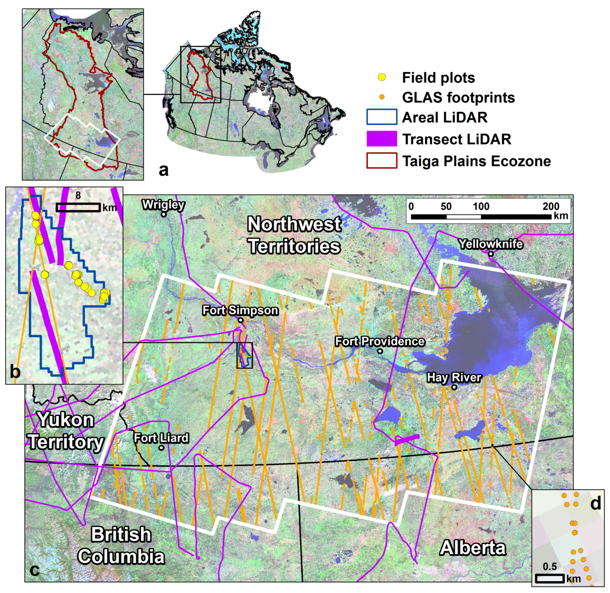
2.1. Study Area
2.2. Field Data
2.3. Airborne LiDAR Data
2.4. GLAS Data
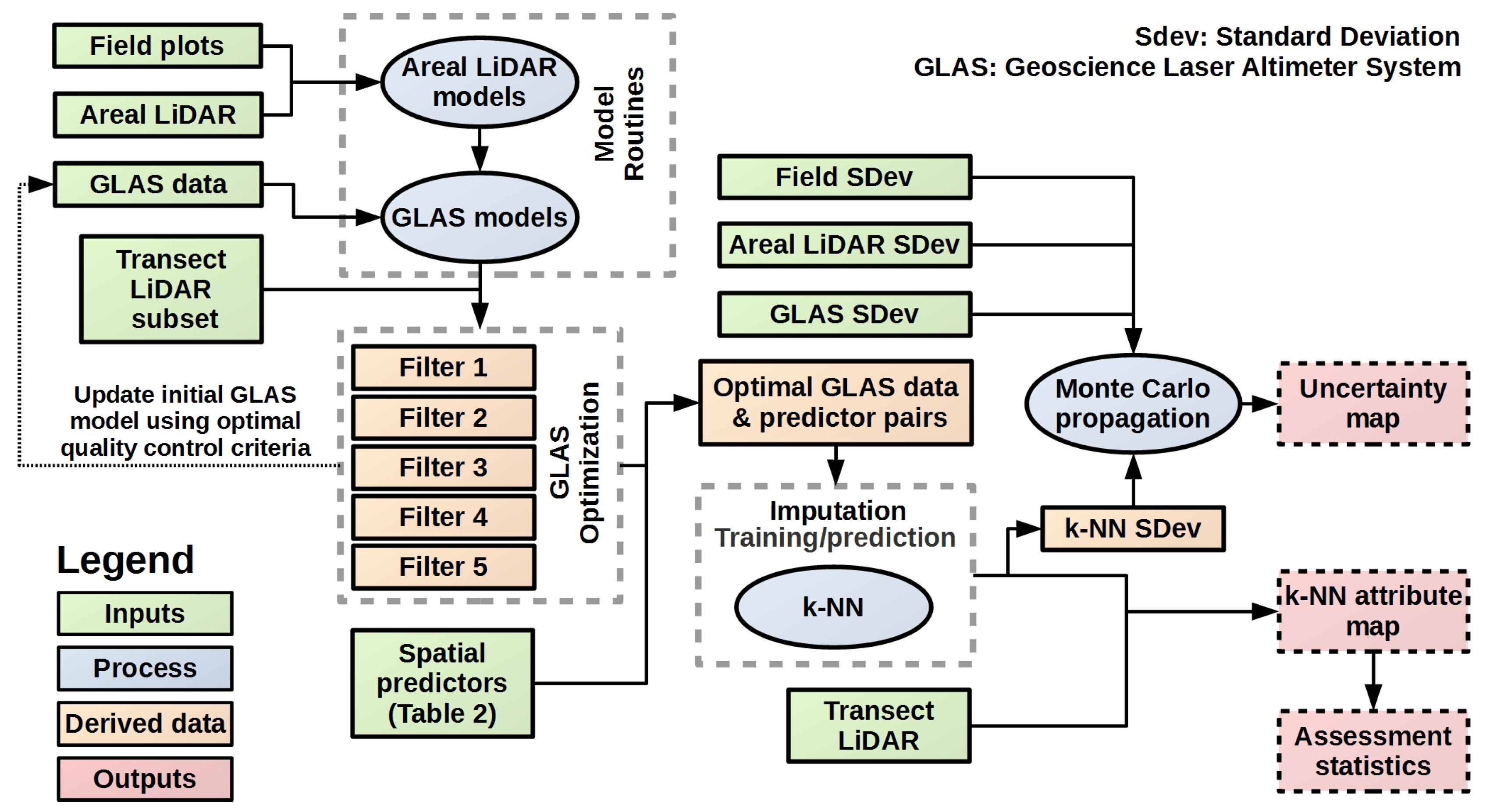
3. Methods
3.1. Airborne LiDAR Models
3.2. GLAS Models
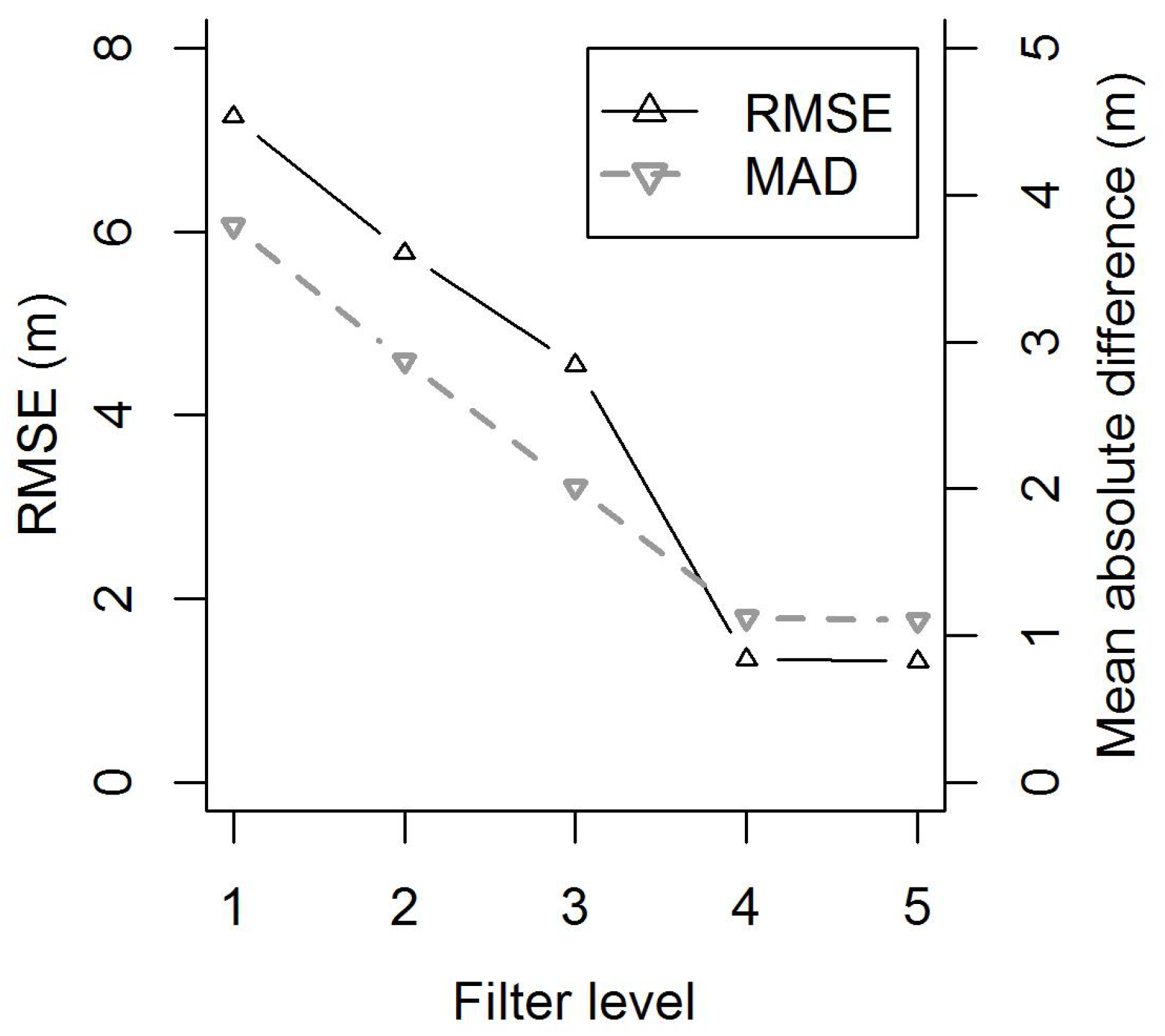
3.2.1. Determining Optimal GLAS Quality Control
3.2.2. GLAS Model Development
3.3. Regional Mapping
3.4. Uncertainties
3.5. Regional Attribute Assessment
4. Results
4.1. Airborne LiDAR Models
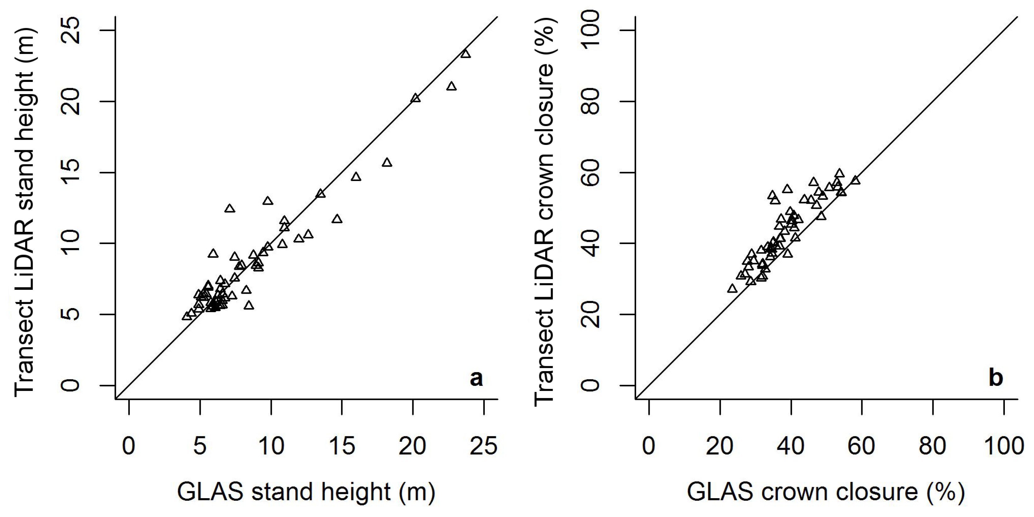
4.2. GLAS Models
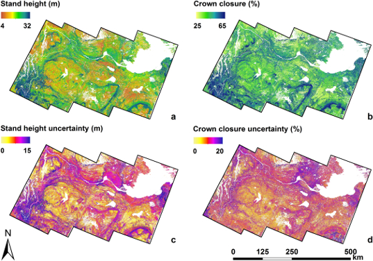
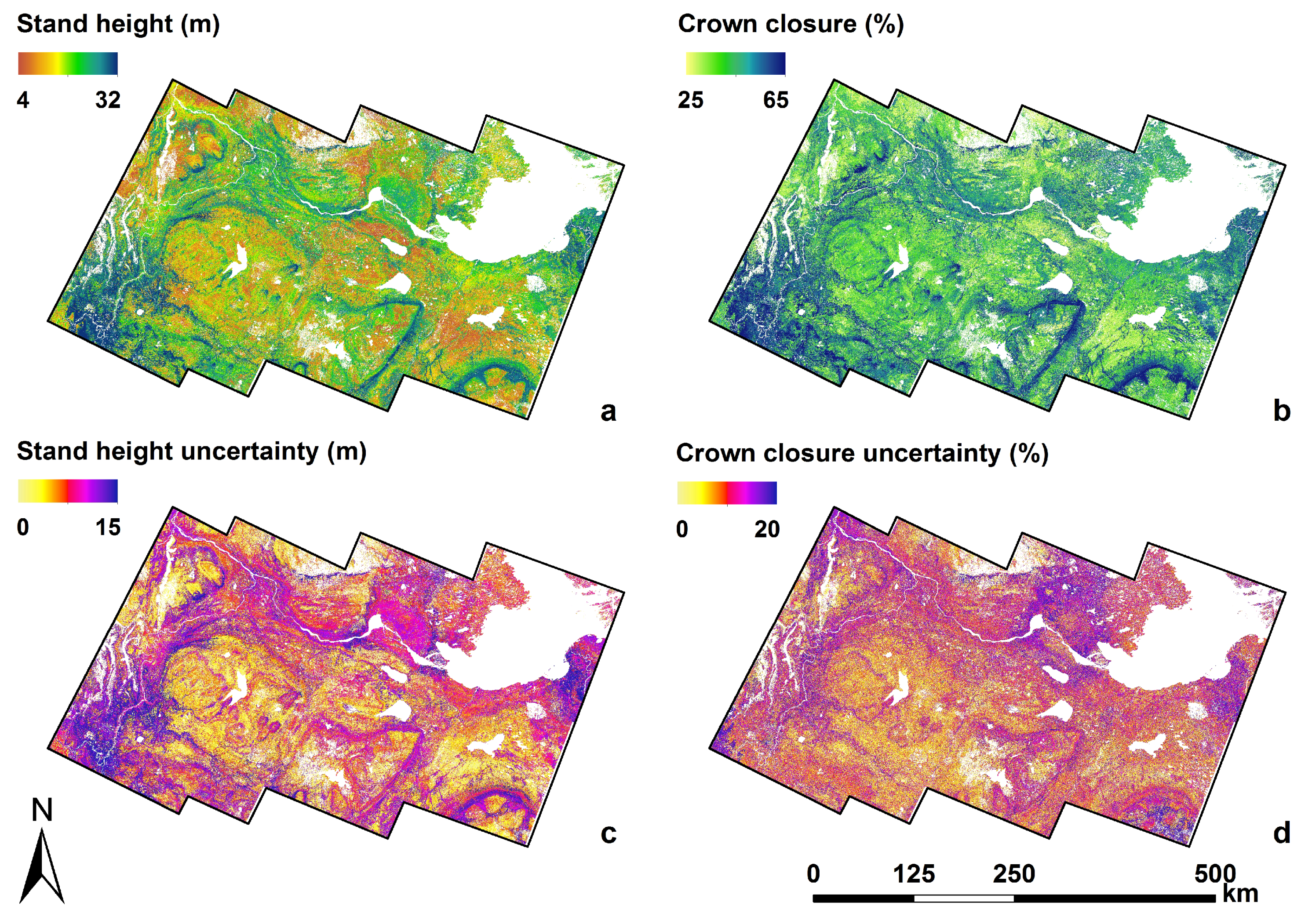
4.3. Regional Mapping and Uncertainties
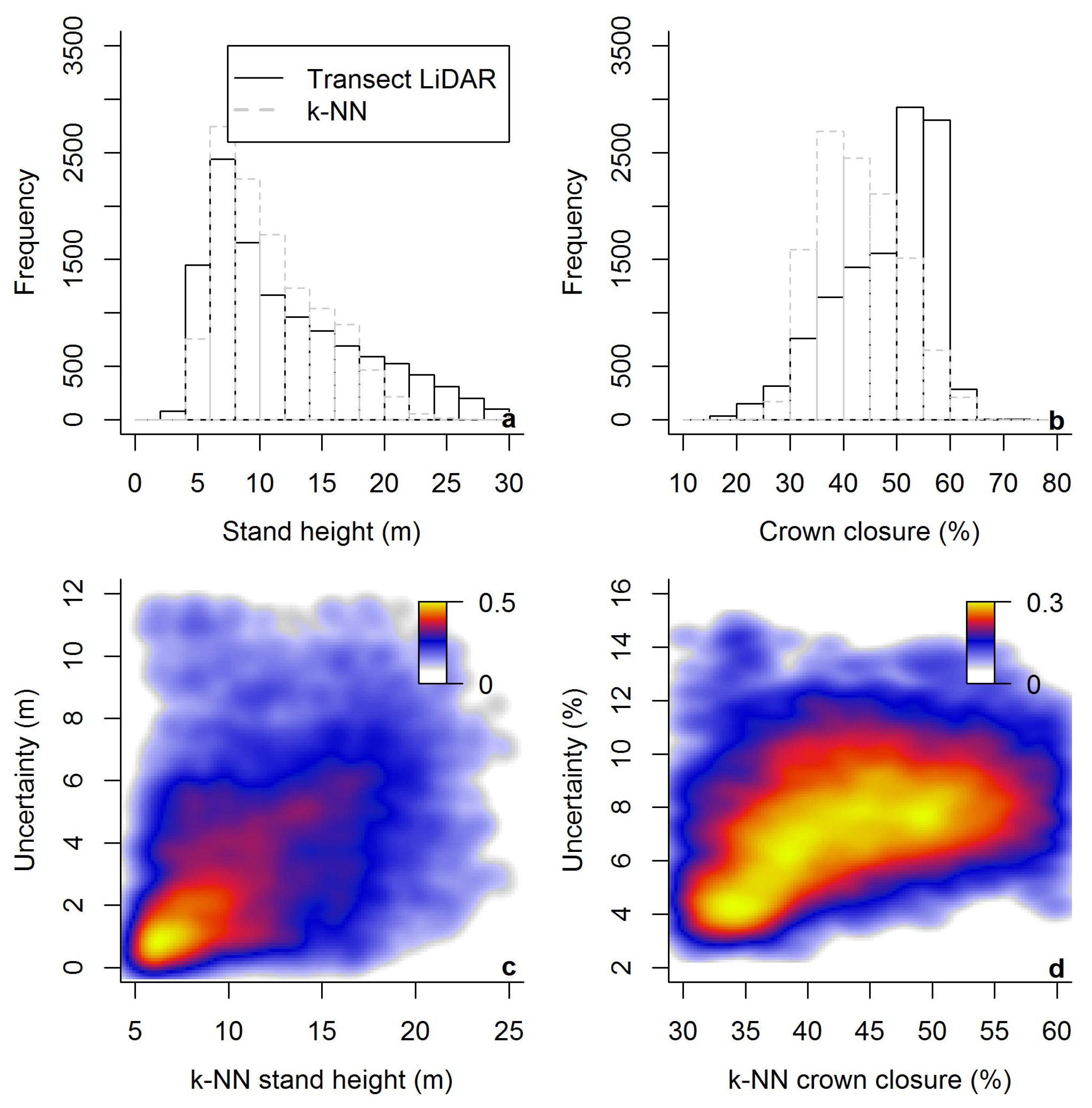
4.4. Regional Attribute Assessment
5. Discussion
5.1. How Did the Methods Framework Compare to Published Studies?
5.2. How Did the Accuracy and Uncertainty Estimates Achieved Compare to Other Studies?
5.3. What Are the Limitations and Opportunities for Improvement?
5.4. What Are the Potential Applications of the Products Generated?
6. Conclusions
Supplementary Materials
Author Contributions
Funding
Acknowledgments
Conflicts of Interest
Abbreviations
| CDEM | Canadian Digital Elevation Model |
| EOSD | Earth Observation for Sustainable Development of Forests |
| GLAS | Geoscience Laser Altimeter System |
| k-NN | k Nearest Neighbour |
| LiDAR | Light Detection And Ranging |
| MAD | Mean Absolute Difference |
| MPE | Mean Prediction Error |
| NDVI | Normalized Difference Vegetation Index |
| NDMI | Normalized Difference Moisture Index |
| SAVI | Soil Adjusted Vegetation Index |
| NWT | Northwest Territories |
| PRF | Pulse Repetition Frequency |
| RMSE | Root Mean Squared Error |
References
- Winton, M. Amplified Arctic climate change: What does surface albedo feedback have to do with it? Geophys. Res. Lett. 2006, 33, L03701. [Google Scholar] [CrossRef]
- IPCC. Contribution of working group I to the Fifth Assessment Report of the Intergovernmental Panel on Climate Change. In IPCC: Climate Change 2013: The Physical Science Basis; Stocker, T., Qin, D., Plattner, G., Tignor, M., Allen, S., Boschung, J., Nauels, A., Xia, Y., Bex, B., Midgley, B., Eds.; Cambridge University Press: Cambridge, UK; New York, NY, USA, 2013; pp. 33–115. [Google Scholar]
- IPCC. Contribution of working group III to the Fifth Assessment Report of the Intergovernmental Panel on Climate Change. In IPCC: Climate Change 2014: Mitigation of Climate Change; Edenhofer, O., Pichs-Madruga, R., Sokona, Y., Minx, J., Farahani, E., Kadner, S., Seyboth, K., Adler, A., Baum, I., Brunner, S., et al., Eds.; Cambridge University Press: New York, NY, USA, 2014; pp. 1–99. [Google Scholar]
- Brandt, J.P. The extent of the North American boreal zone. Environ. Rev. 2009, 17, 101–161. [Google Scholar] [CrossRef]
- Natural Resources Canada. 8 Facts about Canada’s Boreal Forest. 2015. Available online: http://www.nrcan.gc.ca/forests/boreal/17394 (accessed on 25 October 2016).
- Helbig, M.; Pappas, C.; Sonnentag, O. Permafrost thaw and wildfire: Equally important drivers of boreal tree cover changes in the Taiga Plains, Canada. Geophys. Res. Lett. 2016, 43, 1598–1606. [Google Scholar] [CrossRef]
- Gillis, M.D. Canada’s National Forest Inventory (Responding to Current Information Needs). Environ. Monit. Assess. 2001, 67, 121–129. [Google Scholar] [CrossRef] [PubMed]
- Wulder, M.A.; Kurz, W.A.; Gillis, M. National level forest monitoring and modelling in Canada. Prog. Plan. 2004, 61, 365–381. [Google Scholar] [CrossRef]
- Gillis, M.D.; Omule, A.Y.; Brierley, T. Monitoring Canada’s forests: The National Forest Inventory. For. Chron. 2005, 81, 214–221. [Google Scholar] [CrossRef]
- Leckie, D.G.; Gillis, M.D. Forest inventory in Canada with emphasis on map production. For. Chron. 1995, 71, 74–88. [Google Scholar] [CrossRef] [Green Version]
- Hall, R.J. The Roles of Aerial Photographs in Forestry Remote Sensing Image Analysis. In Remote Sensing of Forest Environments; Wulder, M.A., Franklin, S.E., Eds.; Springer: New York, NY, USA, 2003; Chapter 3; pp. 47–75. [Google Scholar]
- Magnusson, M.; Fransson, J.E.S.; Olsson, H. Aerial photo-interpretation using Z/I DMC images for estimation of forest variables. Scand. J. For. Res. 2007, 22, 254–266. [Google Scholar] [CrossRef]
- Smith, L. Forest Resource Inventory and Analysis Strategic Plan; Hay River, NT, Canada, 2002. [Google Scholar]
- Pflugmacher, D.; Cohen, W.; Kennedy, R.; Lefsky, M. Regional Applicability of Forest Height and Aboveground Biomass Models for the Geoscience Laser Altimeter System. For. Sci. 2008, 54, 647–657. [Google Scholar]
- Wulder, M.A.; Dechka, J.A.; Gillis, M.A.; Luther, J.E.; Hall, R.J.; Beaudoin, A.; Franklin, S.E. Operational mapping of the land cover of the forested area of Canada with Landsat data: EOSD land cover program. For. Chron. 2003, 79, 1075–1083. [Google Scholar] [CrossRef] [Green Version]
- Hall, R.J.; Skakun, R.S.; Filiatrault, M.; Gartrell, M.; Arsenault, E.J.; Voicu, M. Multi-Sensor Remote Sensing Data for Forest Inventory: Extending the Value of Satellite Land Cover Maps; Technical Report 1; Natural Resoucres Canada: Edmonton, AB, Canada, 2012.
- Gauthier, S.; Bernier, P.; Kuuluvainen, T.; Shvidenko, A.Z.; Schepaschenko, D.G. Boreal forest health and global change. Science 2015, 349, 819–822. [Google Scholar] [CrossRef] [PubMed]
- Nelson, R.; Krabill, W.; MacLean, G. Determining forest canopy characteristics using airborne laser data. Remote Sens. Environ. 1984, 15, 201–212. [Google Scholar] [CrossRef]
- Lefsky, M.A.; Cohen, W.B.; Parker, G.G.; Harding, D.J. Lidar remote sensing for ecosystem studies. Bioscience 2002, 52, 19–30. [Google Scholar] [CrossRef]
- Boudreau, J.; Nelson, R.F.; Margolis, H.A.; Beaudoin, A.; Guindon, L.; Kimes, D.S. Regional aboveground forest biomass using airborne and spaceborne LiDAR in Québec. Remote Sens. Environ. 2008, 112, 3876–3890. [Google Scholar] [CrossRef]
- Rosette, J.A.B.; North, P.R.J.; Suarez, J.C. Vegetation height estimates for a mixed temperate forest using satellite laser altimetry. Int. J. Remote Sens. 2008, 29, 1475–1493. [Google Scholar] [CrossRef]
- Wulder, M.A.; White, J.C.; Nelson, R.F.; Næsset, E.; Ørka, H.O.; Coops, N.C.; Hilker, T.; Bater, C.W.; Gobakken, T. Lidar sampling for large-area forest characterization: A review. Remote Sens. Environ. 2012, 121, 196–209. [Google Scholar] [CrossRef]
- Hopkinson, C.; Chasmer, L.; Colville, D.; Fournier, R.A.; Hall, R.J.; Luther, J.E.; Milne, T.; Petrone, R.M.; St-Onge, B. Moving Toward Consistent ALS Monitoring of Forest Attributes across Canada. Photogramm. Eng. Remote Sens. 2013, 79, 159–173. [Google Scholar] [CrossRef]
- Mahoney, C.; Kljun, N.; Los, S.O.; Chasmer, L.; Hacker, J.M.; Hopkinson, C.; North, P.R.J.; Rosette, J.A.B.; van Gorsel, E. Slope Estimation from ICESat/GLAS. Remote Sens. 2014, 6, 10051–10069. [Google Scholar] [CrossRef] [Green Version]
- Nelson, R.; Boudreau, J.; Gregoire, T.G.; Margolis, H.; Næsset, E.; Gobakken, T.; Ståhl, G. Estimating Quebec provincial forest resources using ICESat/GLAS. Can. J. For. Res. 2009, 39, 862–881. [Google Scholar] [CrossRef]
- Nelson, R.; Ranson, K.J.; Sun, G.; Kimes, D.S.; Kharuk, V.; Montesano, P. Estimating Siberian timber volume using MODIS and ICESat/GLAS. Remote Sens. Environ. 2009, 113, 691–701. [Google Scholar] [CrossRef]
- Beaudoin, A.; Bernier, P.Y.; Guindon, L.; Villemaire, P.; Guo, X.J.; Stinson, G.; Bergeron, T.; Magnussen, S.; Hall, R.J. Mapping attributes of Canada’s forests at moderate resolution through kNN and MODIS imagery. Can. J. For. Res. 2014, 44, 521–532. [Google Scholar] [CrossRef]
- Margolis, H.A.; Nelson, R.F.; Montesano, P.M.; Beaudoin, A.; Sun, G.; Andersen, H.E.; Wulder, M.A. Combining satellite lidar, airborne lidar, and ground plots to estimate the amount and distribution of aboveground biomass in the boreal forest of North America. Can. J. For. Res. 2015, 45, 838–855. [Google Scholar] [CrossRef] [Green Version]
- Mahoney, C.; Hopkinson, C. Continental Estimates of Canopy Gap Fraction by Active Remote Sensing. Can. J. Remote Sens. 2017, 43, 345–359. [Google Scholar] [CrossRef]
- Nilsson, M.; Nordkvist, K.; Jonzén, J.; Lindgren, N.; Axensten, P.; Wallerman, J.; Egberth, M.; Larsson, S.; Nilsson, L.; Eriksson, J.; et al. A nationwide forest attribute map of Sweden predicted using airborne laser scanning data and field data from the National Forest Inventory. Remote Sens. Environ. 2017, 194, 447–454. [Google Scholar] [CrossRef]
- Matasci, G.; Hermosilla, T.; Wulder, M.A.; White, J.C.; Coops, N.C.; Hobart, G.W.; Zald, H.S.J. Large-area mapping of Canadian boreal forest cover, height, biomass and other structural attributes using Landsat composites and lidar plots. Remote Sens. Environ. 2018, 209, 90–106. [Google Scholar] [CrossRef]
- TERN. The Terrestrial Ecosystem Research Network. 2017. Available online: http://www.tern.org.au/ (accessed on 16 December 2017).
- Gillis, M.D.; Leckie, D.G. Forest Inventory Mapping Procedures across Canada; Forestry Canada Information Rep. PI-X-114; Petawawa National Forestry Institute: Chalk River, ON, Canada, 1993. [Google Scholar]
- Government of Northwest Territories. Northwest Territories Forest Vegetation Inventory Standards with Softcopy Supplements, v4.0; Technical Report; Government of Northwest Territories: Yellowknife, NT, Canada, 2012.
- Ecosystem Classification Group. Ecological Regions of the Northwest Territories–Taiga Plains; Technical Report; Department of Environment and Natural Resources, Government of the Northwest Territories: Yellowknife, NT, Canada, 2007.
- Ecological Stratification Working Group. A National Ecological Framework for Canada; Technical Report; Government of Canada: Ottawa, ON, Canada, 1996.
- Philip, M.S. Measuring Trees and Forests; CAB International: Wallingford, UK, 1994. [Google Scholar]
- Lemmon, P.E. A spherical densiometer for estimating forest overstory density. For. Sci. 1956, 2, 314–320. [Google Scholar]
- Wulder, M.A.; White, J.C.; Bater, C.W.; Coops, N.C.; Hopkinson, C.; Chen, G. Lidar plots—A new large-area data collection option: Context, concepts, and case study. Can. J. Remote Sens. 2012, 38, 600–618. [Google Scholar] [CrossRef]
- Hopkinson, C.; Colvile, D.; Bourdeau, D.; Monette, S.; Maher, R. Scaling plot to stand-level lidar to province in a hierarchical approach to map forest biomass in Nova Scotia. In Proceedings of the 11th International Conference on LiDAR Applications for Assessing Forest Ecosystems, SilviLaser 2011, Hobart, Australia, 16–20 October 2011. [Google Scholar]
- Holmgren, J.; Nilsson, M.; Olsson, H. Simulating the effects of lidar scanning angle for estimation of mean tree height and canopy closure. Can. J. Remote Sens. 2003, 29, 623–632. [Google Scholar] [CrossRef]
- Hopkinson, C. The influence of flying altitude, beam divergence, and pulse repetition frequency on laser pulse return intensity and canopy frequency distribution. Can. J. Remote Sens. 2007, 33, 312–324. [Google Scholar] [CrossRef]
- Morsdorf, F.; Frey, O.; Meier, E.; Itten, K.I.; Allgöwer, B. Assessment of the influence of flying altitude and scan angle on biophysical vegetation products derived from airborne laser scanning. Int. J. Remote Sens. 2008, 29, 1387–1406. [Google Scholar] [CrossRef]
- Bolton, D.K.; Coops, N.C.; Wulder, M.A. Measuring forest structure along productivity gradients in the Canadian boreal with small-footprint Lidar. Environ. Monit. Assess. 2013, 185, 6617–6634. [Google Scholar] [CrossRef] [PubMed]
- Zald, H.S.J.; Wulder, M.A.; White, J.C.; Hilker, T.; Hermosilla, T.; Hobart, G.W.; Coops, N.C. Integrating Landsat pixel composites and change metrics with lidar plots to predictively map forest structure and aboveground biomass in Saskatchewan, Canada. Remote Sens. Environ. 2016, 176, 188–201. [Google Scholar] [CrossRef]
- McGaughey, R. FUSION/LDV: Software for LIDAR Data Analysis and Visualization (Version 3.60+); Technical Report, US Department of Agriculture, Forest Service, Pacific Northwest Research Station: Seattle, WA, USA, 2012.
- Brenner, A.; Zwally, H.; Bentley, C.; Csathó, B.; Harding, D.; Hofton, M.; Minster, J.; Roberts, L.; Saba, J.; Thomas, R.; et al. Geoscience Laser Altimeter System (GLAS) Algorithm Theoretical Basis Document 4.1: Derivation of Range and Range Distributions From Laser Pulse Waveform Analysis for Surface Elevations, Roughness, Slope, and Vegetation Heights; Technical Report; National Aeronautics and Space Administration, Goddard Space Flight Center: Greenbelt, MD, USA, 2003.
- Zwally, H.; Schutz, B.; Bentley, C.; Bufton, J.; Herring, T.; Minster, J.; Spinhirne, J.; Thomas, R. GLAS/ICESat L2 Global Land Surface Altimetry Data, Version 33; National Snow and Ice Data Center (NSIDC): Boulder, CO, USA, 2011. [Google Scholar]
- Hayashi, M.; Saigusa, N.; Oguma, H.; Yamagata, Y. Forest canopy height estimation using ICESat/GLAS data and error factor analysis in Hokkaido, Japan. ISPRS J. Photogramm. Remote Sens. 2013, 81, 12–18. [Google Scholar] [CrossRef]
- Schutz, B.E.; Zwally, H.J.; Shuman, C.A.; Hancock, D.; DiMarzio, J.P. Overview of the ICESat Mission. Geophys. Res. Lett. 2005, 32, L21S01. [Google Scholar] [CrossRef]
- Neuenschwander, A.L.; Urban, T.J.; Gutierrez, R.; Schutz, B.E. Characterization of ICESat/GLAS waveforms over terrestrial ecosystems: Implications for vegetation mapping. J. Geophys. Res.-Biogeosci. 2008, 113, G02S03. [Google Scholar] [CrossRef]
- Miller, M.E.; Lefsky, M.; Pang, Y. Optimization of Geoscience Laser Altimeter System waveform metrics to support vegetation measurements. Remote Sens. Environ. 2011, 115, 298–305. [Google Scholar] [CrossRef]
- Mahoney, C.; Hopkinson, C.; Kljun, N.; Van Gorsel, E. ICESat/GLAS canopy height sensitivity inferred from airborne LiDAR. Photogramm. Eng. Remote Sens. 2016, 82, 351–363. [Google Scholar] [CrossRef]
- Mora, B.; Wulder, M.; White, J.; Hobart, G. Modeling Stand Height, Volume, and Biomass from Very High Spatial Resolution Satellite Imagery and Samples of Airborne LiDAR. Remote Sens. 2013, 5, 2308–2326. [Google Scholar] [CrossRef] [Green Version]
- Lovell, J.L.; Jupp, D.L.B.; Culvenor, D.S.; Coops, N.C. Using airborne and ground-based ranging lidar to measure canopy structure in Australian forests. Can. J. Remote Sens. 2003, 29, 607–622. [Google Scholar] [CrossRef]
- Riano, D.; Meier, E.; Allgöwer, B.; Chuvieco, E.; Ustin, S.L. Modeling airborne laser scanning data for the spatial generation of critical forest parameters in fire behavior modeling. Remote Sens. Environ. 2003, 86, 177–186. [Google Scholar] [CrossRef]
- Coops, N.C.; Hilker, T.; Wulder, M.A.; St-Onge, B.; Newnham, G.; Siggins, A.; Trofymow, J.T. Estimating canopy structure of Douglas-fir forest stands from discrete-return LiDAR. Trees 2007, 21, 295–310. [Google Scholar] [CrossRef] [Green Version]
- Lefsky, M.A.; Keller, M.; Pang, Y.; de Camargo, P.B.; Hunter, M.O. Revised method for forest canopy height estimation from Geoscience Laser Altimeter System waveforms. J. Appl. Remote Sens. 2007, 1, 013537. [Google Scholar]
- Pang, Y.; Lefsky, M.; Andersen, H.E.; Miller, M.E.; Sherrill, K. Validation of the ICEsat vegetation product using crown-area-weighted mean height derived using crown delineation with discrete return lidar data. Can. J. Remote Sens. 2008, 34, S471–S484. [Google Scholar] [CrossRef]
- Chen, Q. Retrieving vegetation height of forests and woodlands over mountainous areas in the Pacific Coast region using satellite laser altimetry. Remote Sens. Environ. 2010, 114, 1610–1627. [Google Scholar] [CrossRef]
- Park, T.; Kennedy, R.; Choi, S.; Wu, J.; Lefsky, M.; Bi, J.; Mantooth, J.; Myneni, R.; Knyazikhin, Y. Application of Physically-Based Slope Correction for Maximum Forest Canopy Height Estimation Using Waveform Lidar across Different Footprint Sizes and Locations: Tests on LVIS and GLAS. Remote Sens. 2014, 6, 6566–6586. [Google Scholar] [CrossRef] [Green Version]
- Simard, M.; Pinto, N.; Fisher, J.B.; Baccini, A. Mapping forest canopy height globally with spaceborne lidar. J. Geophys. Res.-Biogeosci. 2011, 116, G04021. [Google Scholar] [CrossRef]
- Environment and Climate Change Canada. Historical Climate Data. 2017. Available online: http://climate.weather.gc.ca/ (accessed on 30 September 2015).
- Harding, D.J.; Lefsky, M.A.; Parker, G.G.; Blair, J.B. Laser altimeter canopy height profiles: Methods and validation for closed-canopy, broadleaf forests. Remote Sens. Environ. 2001, 76, 283–297. [Google Scholar] [CrossRef]
- Hall, R.J.; Skakun, R.S.; Arsenault, E.J.; Gartrell, M.; Simpson, B.; Filiatrault, M. Multi-Sensor Remote Sensing Data for Forest Inventory: Extending the Value of Satellite Land Cover Maps; Technical Report 1; Natural Resoucres Canada: Edmonton, AB, Canada, 2009.
- McRoberts, R.E.; Nelson, M.D.; Wendt, D.G. Stratified estimation of forest area using satellite imagery, inventory data, and the k-Nearest Neighbors technique. Remote Sens. Environ. 2002, 82, 457–468. [Google Scholar] [CrossRef]
- McRoberts, R.E.; Næsset, E.; Gobakken, T. Optimizing the k-Nearest Neighbors technique for estimating forest aboveground biomass using airborne laser scanning data. Remote Sens. Environ. 2015, 163, 13–22. [Google Scholar] [CrossRef]
- Chirici, G.; Mura, M.; McInerney, D.; Py, N.; Tomppo, E.O.; Waser, L.T.; Travaglini, D.; McRoberts, R.E. A meta-analysis and review of the literature on the k-Nearest Neighbors technique for forestry applications that use remotely sensed data. Remote Sens. Environ. 2016, 176, 282–294. [Google Scholar] [CrossRef]
- Altman, N.S. An Introduction to Kernel and Nearest-Neighbor Nonparametric Regression. Am. Stat. 1992, 46, 175–185. [Google Scholar] [Green Version]
- NASA. NASA Landsat Program, Landsat ETM+; U. S. Geological Survey: Reston, VA, USA, 2003.
- Hall, R.J.; Skakun, R.S.; Arsenault, E.J.; Case, B.S. Modeling forest stand structure attributes using Landsat ETM+ data: Application to mapping of aboveground biomass and stand volume. For. Ecol. Manag. 2006, 225, 378–390. [Google Scholar] [CrossRef]
- Zheng, D.; Rademacher, J.; Chen, J.; Crow, T.; Bresee, M.; Moine, J.L.; Ryu, S.R. Estimating aboveground biomass using Landsat 7 ETM+ data across a managed landscape in northern Wisconsin, USA. Remote Sens. Environ. 2004, 93, 402–411. [Google Scholar] [CrossRef]
- Klinka, K.; Chen, H.Y.H.; Wang, Q.; Carter, R.E. Height growth–elevation relationships in subalpine forests of interior British Columbia. For. Chron. 1996, 72, 193–198. [Google Scholar] [CrossRef] [Green Version]
- Coombes, D.A.; Allen, R.B. Effects of size, competition and altitude on tree growth. J. Ecol. 2007, 95, 1084–1097. [Google Scholar] [CrossRef] [Green Version]
- Government of Canada. Canadian Digital Elevation Model (CDEM), Version 3.0; Government of Canada: Ottawa, ON, USA, 2012.
- Hogg, E.; Barr, A.; Black, T. A simple soil moisture index for representing multi-year drought impacts on aspen productivity in the western Canadian interior. Agric. For. Meteorol. 2013, 178, 173–182. [Google Scholar] [CrossRef]
- Beven, K.J.; Kirkby, M.J. A physically based, variable contributing area model of basin hydrology/Un modèle à base physique de zone d’appel variable de l’hydrologie du bassin versant. Hydrol. Sci. Bull. 1979, 24, 43–69. [Google Scholar] [CrossRef]
- Gessler, P.E.; Chadwick, O.A.; Chamran, F.; Althouse, L.; Holmes, K. Modeling Soil-Landscape and Ecosystem Properties Using Terrain Attributes. Soil Sci. Soc. Am. J. 2000, 64, 2046–2056. [Google Scholar] [CrossRef]
- Dong, J.; Kaufmann, R.K.; Myneni, R.B.; Tucker, C.J.; Kauppi, P.E.; Liski, J.; Buermann, W.; Alexeyev, V.; Hughes, M.K. Remote sensing estimates of boreal and temperate forest woody biomass: Carbon pools, sources, and sinks. Remote Sens. Environ. 2003, 84, 393–410. [Google Scholar] [CrossRef]
- Glenn, E.P.; Huete, A.R.; Nagler, P.L.; Nelson, S.G. Relationship Between Remotely-sensed Vegetation Indices, Canopy Attributes and Plant Physiological Processes: What Vegetation Indices Can and Cannot Tell Us About the Landscape. Sensors 2008, 8, 2136–2160. [Google Scholar] [CrossRef] [PubMed] [Green Version]
- Song, C. Optical remote sensing of forest leaf area index and biomass. Prog. Phys. Geogr. Earth Environ. 2013, 37, 98–113. [Google Scholar] [CrossRef]
- Cai, G.B. NDWI–A normalized difference water index for remote sensing of vegetation liquid water from space. Remote Sens. Environ. 1996, 58, 257–266. [Google Scholar]
- Jin, S.; Sader, S.A. Comparison of time series tasseled cap wetness and the normalized difference moisture index in detecting forest disturbances. Remote Sens. Environ. 2005, 94, 364–372. [Google Scholar] [CrossRef]
- Huete, A. A soil-adjusted vegetation index (SAVI). Remote Sens. Environ. 1988, 25, 295–309. [Google Scholar] [CrossRef]
- Asner, G.P.; Hicke, J.A.; Lobell, D.B. Per-Pixel Analysis of Forest Structure. In Remote Sensing of Forest Environments: Concepts and Case Studies; Wulder, M.A., Franklin, S.E., Eds.; Springer: Boston, MA, USA, 2003; pp. 209–254. [Google Scholar]
- Hechenbichler, K.; Schliep, K. Weighted k-Nearest-Neighbor Techniques and Ordinal Classification; Discussion Paper 399, SFB 386; Ludwig-Maximilians University: Munchen, Germany, 2004. [Google Scholar]
- Kruskal, J.B. Multidimensional scaling by optimizing goodness of fit to a nonmetric hypothesis. Psychometrika 1964, 29, 1–27. [Google Scholar] [CrossRef]
- Samworth, R.J. Optimal weighted nearest neighbour classifiers. Ann. Stat. 2012, 40, 2733–2763. [Google Scholar] [CrossRef]
- Chen, Q.; McRoberts, R.E.; Wang, C.; Radtke, P.J. Forest aboveground biomass mapping and estimation across multiple spatial scales using model-based inference. Remote Sens. Environ. 2016, 184, 350–360. [Google Scholar] [CrossRef]
- Hammersley, J.M.; Handscomb, D.C. Monte Carlo Methods; Chapman and Hall: London, UK, 1964. [Google Scholar]
- Ogilvie, J.F. A monte-carlo approach to error propagation. Comput. Chem. 1984, 8, 205–207. [Google Scholar] [CrossRef]
- Anderson, G. Error propagation by the Monte Carlo method in geochemical calculations. Geochim. Cosmochim. Acta 1976, 40, 1533–1538. [Google Scholar] [CrossRef]
- Mudron, I.; Podhoranyi, M.; Cirbus, J.; Devecka, B.; Bakay, L. Modelling the uncertainty of slope estimation from a LiDAR-derived DEM: A case study from a large-scale area in the Czech Republic. Geosci. Eng. 2013, 59, 25–39. [Google Scholar] [CrossRef]
- Ottlé, C.; Mahfouf, J.F. 8–Data Assimilation of Satellite Observations. In Microwave Remote Sensing of Land Surface; Baghdadi, N., Zribi, M., Eds.; Elsevier: New York, NY, USA, 2016; pp. 357–382. [Google Scholar]
- Cohen, J. Statistical power analysis. Curr. Direct. Psychol. Sci. 1992, 1, 98–101. [Google Scholar] [CrossRef]
- Thomas, V.; Treitz, P.; McCaughey, J.H.; Morrison, I. Mapping stand-level forest biophysical variables for a mixedwood boreal forest using lidar: An examination of scanning density. Can. J. For. Res. 2006, 36, 34–47. [Google Scholar] [CrossRef]
- Korhonen, L.; Korpela, I.; Heiskanen, J.; Maltamo, M. Airborne discrete-return LIDAR data in the estimation of vertical canopy cover, angular canopy closure and leaf area index. Remote Sens. Environ. 2011, 115, 1065–1080. [Google Scholar] [CrossRef]
- Korhonen, L.; Korhonen, K.; Rautiainen, M.; Stenberg, P. Estimation of forest canopy cover: A comparison of field measurement techniques. Silva Fenn. 2006, 40, 577–588. [Google Scholar] [CrossRef]
- Saatchi, S.S.; Harris, N.L.; Brown, S.; Lefsky, M.; Mitchard, E.T.A.; Salas, W.; Zutta, B.R.; Buermann, W.; Lewis, S.L.; Hagen, S.; et al. Benchmark map of forest carbon stocks in tropical regions across three continents. Proc. Natl. Acad. Sci. USA 2011, 108, 9899–9904. [Google Scholar] [CrossRef] [PubMed] [Green Version]
- McRoberts, R.E.; Tomppo, E.O. Remote sensing support for national forest inventories. Remote Sens. Environ. 2007, 110, 412–419. [Google Scholar] [CrossRef]
- Chirici, G.; Barbati, A.; Corona, P.; Marchetti, M.; Travaglini, D.; Maselli, F.; Bertini, R. Non-parametric and parametric methods using satellite images for estimating growing stock volume in alpine and Mediterranean forest ecosystems. Remote Sens. Environ. 2008, 112, 2686–2700. [Google Scholar] [CrossRef] [Green Version]
- Baffetta, F.; Fattorini, L.; Franceschi, S.; Corona, P. Design-based approach to k-nearest neighbours technique for coupling field and remotely sensed data in forest surveys. Remote Sens. Environ. 2009, 113, 463–475. [Google Scholar] [CrossRef] [Green Version]
- Tian, X.; Li, Z.; Su, Z.; Chen, E.; van der Tol, C.; Li, X.; Guo, Y.; Li, L.; Ling, F. Estimating montane forest above-ground biomass in the upper reaches of the Heihe River Basin using Landsat-TM data. Int. J. Remote Sens. 2014, 35, 7339–7362. [Google Scholar] [CrossRef]
- Gjertsen, A.K. Accuracy of forest mapping based on Landsat TM data and a kNN-based method. Remote Sens. Environ. 2007, 110, 420–430. [Google Scholar] [CrossRef]
- Bolton, D.K.; Coops, N.C.; Wulder, M.A. Investigating the agreement between global canopy height maps and airborne Lidar derived height estimates over Canada. Can. J. Remote Sens. 2013, 39, S139–S151. [Google Scholar] [CrossRef]
- Lefsky, M.A. A global forest canopy height map from the Moderate Resolution Imaging Spectroradiometer and the Geoscience Laser Altimeter System. Geophys. Res. Lett. 2010, 37. [Google Scholar] [CrossRef] [Green Version]
- Nelson, R.; Gobakken, T.; Næsset, E.; Gregoire, T.; Ståhl, G.; Holm, S.; Flewelling, J. Lidar sampling—Using an airborne profiler to estimate forest biomass in Hedmark County, Norway. Remote Sens. Environ. 2012, 123, 563–578. [Google Scholar] [CrossRef]
- McRoberts, R.E.; Chen, Q.; Gormanson, D.D.; Walters, B.F. The shelf-life of airborne laser scanning data for enhancing forest inventory inferences. Remote Sens. Environ. 2018, 206, 254–259. [Google Scholar] [CrossRef]
- Liu, J.; Chen, J.M.; Cihlar, J.; Chen, W. Net primary productivity mapped for Canada at 1-km resolution. Glob. Ecol. Biogeogr. 2002, 11, 115–129. [Google Scholar] [CrossRef]
- Neigh, C.S.; Nelson, R.F.; Ranson, K.J.; Margolis, H.A.; Montesano, P.M.; Sun, G.; Kharuk, V.; Næsset, E.; Wulder, M.A.; Andersen, H.E. Taking stock of circumboreal forest carbon with ground measurements, airborne and spaceborne LiDAR. Remote Sens. Environ. 2013, 137, 274–287. [Google Scholar] [CrossRef]
- Ståhl, G.; Holm, S.; Gregoire, T.G.; Gobakken, T.; Næsset, E.; Nelson, R. Model-based inference for biomass estimation in a LiDAR sample survey in Hedmark County, NorwayThis article is one of a selection of papers from Extending Forest Inventory and Monitoring over Space and Time. Can. J. For. Res. 2011, 41, 96–107. [Google Scholar] [CrossRef]
- Nelson, R. Model effects on GLAS-based regional estimates of forest biomass and carbon. Int. J. Remote Sens. 2010, 31, 1359–1372. [Google Scholar] [CrossRef] [Green Version]
- Lutz, D.A.; Washington-Allen, R.A.; Shugart, H.H. Remote sensing of boreal forest biophysical and inventory parameters: A review. Can. J. Remote Sens. 2008, 34, S286–S313. [Google Scholar] [CrossRef]
- Fiala, A.C.; Garman, S.L.; Gray, A.N. Comparison of five canopy cover estimation techniques in the western Oregon Cascades. For. Ecol. Manag. 2006, 232, 188–197. [Google Scholar] [CrossRef]
- Smith, A.M.; Falkowski, M.J.; Hudak, A.T.; Evans, J.S.; Robinson, A.P.; Steele, C.M. A cross-comparison of field, spectral, and lidar estimates of forest canopy cover. Can. J. Remote Sens. 2009, 35, 447–459. [Google Scholar] [CrossRef]
- Beaudoin, A.; Bernier, P.; Villemaire, P.; Guindon, L.; Guo, X.J. Tracking forest attributes across Canada between 2001 and 2011 using a k nearest neighbors mapping approach applied to MODIS imagery. Can. J. For. Res. 2017, 48, 85–93. [Google Scholar] [CrossRef]
- Mitchard, E.T.A.; Saatchi, S.S.; Woodhouse, I.H.; Nangendo, G.; Ribeiro, N.S.; Williams, M.; Ryan, C.M.; Lewis, S.L.; Feldpausch, T.R.; Meir, P. Using satellite radar backscatter to predict above-ground woody biomass: A consistent relationship across four different African landscapes. Geophys. Res. Lett. 2009, 36, L23401. [Google Scholar] [CrossRef]
- Cartus, O.; Santoro, M.; Kellndorfer, J. Mapping forest aboveground biomass in the Northeastern United States with ALOS PALSAR dual-polarization L-band. Remote Sens. Environ. 2012, 124, 466–478. [Google Scholar] [CrossRef]
- Lu, D.; Chen, Q.; Wang, G.; Liu, L.; Li, G.; Moran, E. A survey of remote sensing-based aboveground biomass estimation methods in forest ecosystems. Int. J. Digit. Earth 2016, 9, 63–105. [Google Scholar] [CrossRef]
- McRoberts, R.E. Diagnostic tools for nearest neighbors techniques when used with satellite imagery. Remote Sens. Environ. 2009, 113, 489–499. [Google Scholar] [CrossRef]
- Latifi, H.; Koch, B. Evaluation of most similar neighbour and random forest methods for imputing forest inventory variables using data from target and auxiliary stands. Int. J. Remote Sens. 2012, 33, 6668–6694. [Google Scholar] [CrossRef]
- Packalén, P.; Temesgen, H.; Maltamo, M. Variable selection strategies for nearest neighbor imputation methods used in remote sensing based forest inventory. Can. J. Remote Sens. 2012, 38, 557–569. [Google Scholar] [CrossRef]
- Breiman, L. Random forests. Mach. Learn. 2001, 45, 5–32. [Google Scholar] [CrossRef]
- Latifi, H.; Nothdurft, A.; Koch, B. Non-parametric prediction and mapping of standing timber volume and biomass in a temperate forest: Application of multiple optical/LiDAR-derived predictors. For. Int. J. For. Res. 2010, 83, 395–407. [Google Scholar] [CrossRef]
- Shataee, S.; Kalbi, S.; Fallah, A.; Pelz, D. Forest attribute imputation using machine-learning methods and ASTER data: Comparison of k-NN, SVR and random forest regression algorithms. Int. J. Remote Sens. 2012, 33, 6254–6280. [Google Scholar] [CrossRef]
- Hudak, A.T.; Crookston, N.L.; Evans, J.S.; Hall, D.E.; Falkowski, M.J. Nearest neighbor imputation of species-level, plot-scale forest structure attributes from LiDAR data. Remote Sens. Environ. 2008, 112, 2232–2245. [Google Scholar] [CrossRef]
- McInerney, D.O.; Nieuwenhuis, M. A comparative analysis of kNN and decision tree methods for the Irish National Forest Inventory. Int. J. Remote Sens. 2009, 30, 4937–4955. [Google Scholar] [CrossRef]
- Abdalati, W.; Zwally, H.J.; Bindschadler, R.; Csatho, B.; Farrell, S.L.; Fricker, H.A.; Harding, D.; Kwok, R.; Lefsky, M.; Markus, T.; et al. The ICESat-2 Laser Altimetry Mission. Proc. IEEE 2010, 98, 735–751. [Google Scholar] [CrossRef]
- Gauthier, S.; Lorente, M.; Kremsater, L.L.; De Grandpré, L.; Burton, P.J.; Aubin, I.; Hogg, E.H.; Nadeau, S.; Nelson, E.A.; Taylor, A.R.; et al. Tracking Climate Change Effects: Potential Indicators for Canada’s Forests and Forest Sector. Technical Report; Natural Resources Canada–Canadian Forest Service, Laurentian Forestry Centre: Québec, QC, Canada, 2014.
- Environment and Natural Resources. Species at Risk in the NWT; Technical Report; Department of Environment and Natural Resources, Government of Northwest Territories: Yellowknife, NT, Canada, 2018.
- Conference of Management Authorities. Recovery Strategy for the Boreal Caribou (Rangifer tarandus caribou) in the Northwest Territories. Species at Risk (NWT) Act Management Plan and Recovery Strategy Series; Technical Report; Department of Environment and Natural Resources, Government of the Northwest Territories: Yellowknife, NT, Canada, 2017.
- Environment and Natural Resources. NWT Barren-Ground Caribou Management Strategy; Technical Report; Department of Environment and Natural Resources, Government of Northwest Territories: Yellowknife, NT, Canada, 2018.
- McDermid, G.; Hall, R.; Sanchez-Azofeifa, G.; Franklin, S.; Stenhouse, G.; Kobliuk, T.; LeDrew, E. Remote sensing and forest inventory for wildlife habitat assessment. For. Ecol. Manag. 2009, 257, 2262–2269. [Google Scholar] [CrossRef]
- Franklin, S.E. Remote Sensing for Biodiversity and Wildlife Management: Synthesis and Applications; McGraw-Hill: New York, NY, USA, 2010. [Google Scholar]
- Festa-Bianchet, M.; Ray, J.; Boutin, S.; Côté, S.; Gunn, A. Conservation of caribou (Rangifer tarandus) in Canada: An uncertain future. Can. J. Zool. 2011, 89, 419–434. [Google Scholar] [CrossRef]
- Moreau, G.; Fortin, D.; Couturier, S.; Duchesne, T. Multi-level functional responses for wildlife conservation: The case of threatened caribou in managed boreal forests. J. Appl. Ecol. 2012, 49, 611–620. [Google Scholar] [CrossRef]
- Environment and Natural Resources. NWT Biomass Energy Strategy; Technical Report; Department of Environment and Natural Resources, Government of Northwest Territories: Yellowknife, NT, Canada, 2018.
- Flannigan, M.D.; Kochtubajda, B.; Logan, K.A. Forest Fires and Climate Change in the Northwest Territories. In Cold Region Atmospheric and Hydrologic Studies. The Mackenzie GEWEX Experience: Volume 1: Atmospheric Dynamics; Woo, M.k., Ed.; Springer: Berlin/Heidelberg, Germany, 2008; Chapter 23; pp. 403–417. [Google Scholar]
- Popescu, S.C.; Wynne, R.H.; Nelson, R.F. Measuring individual tree crown diameter with lidar and assessing its influence on estimating forest volume and biomass. Can. J. Remote Sens. 2003, 29, 564–577. [Google Scholar] [CrossRef]


| Filter | Description | N | Reference | |||
|---|---|---|---|---|---|---|
| Level 1 | All within study area L2A & L3A available | 0 | 29,268 | 0 | 0 | - |
| Level 2 | Removed saturated, cloud influenced, or footprints with initial height estimates > 35 m | 7000 | 22,268 | −24 | 24 | [20] |
| Level 3 | Removed high slope (>5) and vertical bias from slope > 25% of initial height estimate | 3715 | 18,553 | −37 | 13 | [62] |
| Level 4 | Removed acquisitions made after 22 October 2003 for L2A, and 15 October 2004 for L3A, the first occurrences of snow in the study region for each year | 9155 | 9398 | −67 | 30 | [25] |
| Level 5 | Removed low energy footprints (<28 mJ) in pursuit of highest signal-to-noise ratio | 0 | 9398 | −67 | 0 | [53] |
| Predictor | Native Resolution (m) | Selection Reason(s) | References |
|---|---|---|---|
| EOSD a | 30 | Distinguishes between vegetation types (Coniferous, Deciduous, Mixed, etc.) | [15] |
| Landsat TM Band 3 | 30 | Red: Distinguishing vegetation from soil background. | [27,70,71] |
| Landsat TM Band 4 | 30 | Near infrared (NIR): Indicator of vegetation structure and biomass | [27,70,71,72] |
| Landsat TM Band 5 | 30 | Shortwave infrared (SWIR): Detection of vegetation types and indicator of vegetation and soil moisture content. | [27,70,71] |
| Elevation (source: CDEM b) | 100 | Used as physiographic measure as tree growth is influenced by elevation. | [73,74,75] |
| Climate Moisture Index | 100 | Indicator of moisture availability for plant growth. Computed annually as difference between precipitation and evapotranspiration. | [76] |
| Compound Topographic Index | 100 | Topographic attribute used in soil landscape modelling, indicator of wetness. | [77,78] |
| NDVI | 30 | Computed as difference over sum ratio of Landsat TM bands 4 (NIR) and 3 (red). Used in measures of leaf area index, green vegetation biomass. | [79,80,81] |
| NDMI | 30 | Computed as difference over sum ratio of Landsat TM bands 4 (NIR) and 5 (SWIR). NDMI is correlated to canopy water content. | [82,83] |
| SAVI e | 30 | Similar to NDVI, but reduces effects of soil brightness when vegetation cover is low. | [84,85] |
| Soil Moisture Index | 100 | Direct measure of soil moisture used as an indicator of drought and its effects on vegetation. | [76] |
| Coefficients | ||||||||||
|---|---|---|---|---|---|---|---|---|---|---|
| Attribute (y) | Metric (x) | Units | N | a | b | Adj. R | RMSE | MPE | Min | Max |
| Stand height | p80 | m | 38 | 0.93 | 2.88 | 0.83 | 1.7 | 1.8 | 12.7 | 26.3 |
| p90 | 0.97 | 1.18 | 0.87 | 1.5 | 1.6 | 12.7 | 26.2 | |||
| p95 | 0.96 | 0.53 | 0.89 | 1.4 | 1.4 | 12.2 | 26.0 | |||
| p99 | 0.93 | 0.15 | 0.88 | 1.4 | 1.5 | 11.7 | 27.7 | |||
| Crown closure | Lz | % | 62.78 | 0.25 | 0.63 | 4.8 | 5.0 | 43.5 | 71.1 | |
| Coefficients | |||||||||
|---|---|---|---|---|---|---|---|---|---|
| Attribute (y) | Metric (x) | Units | N | a | b | Adj. R | RMSE | Min | Max |
| Stand height | p85 | m | 43 | 1.10 | 2.30 | 0.88 | 1.3 | 5.8 | 21.5 |
| p90 | 1.03 | 2.08 | 0.88 | 1.3 | 6.1 | 21.2 | |||
| p95 | 0.97 | 1.77 | 0.88 | 1.4 | 6.6 | 20.9 | |||
| p100 | 0.91 | 1.47 | 0.87 | 1.4 | 6.9 | 20.9 | |||
| Crown closure | Lz | % | 64.63 | 0.25 | 0.54 | 6.5 | 31.7 | 62.3 | |
| Statistic | Stand Height (m) | Crown Closure (%) | ||
|---|---|---|---|---|
| GLAS | Transect LiDAR | GLAS | Transect LiDAR | |
| Minimum | 4.1 | 4.8 | 23.4 | 27.1 |
| Maximum | 23.7 | 23.3 | 58.2 | 59.6 |
| Mean | 8.6 | 8.7 | 38.6 | 43.5 |
| Standard deviation | 4.4 | 4.1 | 8.3 | 8.9 |
| Attribute | k | Weighting Kernel | Predictor Set | |
|---|---|---|---|---|
| Stand height | 5(10) | 2 | Inverse distance | EOSD a |
| Landsat TM Band 3 | ||||
| Elevation (CDEM b) | ||||
| Climate moisture index | ||||
| Soil moisture index | ||||
| Crown closure | 5(10) | 1 | Inverse distance | EOSD a |
| Landsat TM Bands 3, 4, 5 | ||||
| Elevation (CDEM a) | ||||
| Climate moisture index | ||||
| Soil moisture index |
| Data Subset | Stand Height (m) | Crown Closure (%) | |||||
|---|---|---|---|---|---|---|---|
| N | MD | MAD | RMSE | MD | MAD | RMSE | |
| Region of interest | 11,401 | −1.1 | 3.7 | 5.1 | −4.9 | 7.4 | 9.2 |
| Coniferous | 8421 | −0.7 | 3.1 | 4.5 | −4.6 | 7.1 | 8.8 |
| Deciduous | 1229 | −2.4 | 5.2 | 6.4 | −3.1 | 7.3 | 9.7 |
| Mixedwood | 1751 | −2.2 | 5.3 | 6.6 | −7.5 | 8.9 | 10.4 |
| Cameron Plateau (LS) | 164 | 1.6 | 2.2 | 2.9 | 0.4 | 4.9 | 6.0 |
| Cameron Slopes (MB) | 303 | −0.2 | 3.6 | 4.6 | −2.8 | 4.8 | 6.2 |
| Ebbutt Upland (HB) | 234 | −2.0 | 3.4 | 4.9 | −10.2 | 11.2 | 13.3 |
| Great Slave Lowland (MB) | 527 | −1.3 | 3.2 | 3.8 | −5.9 | 8.8 | 10.4 |
| Great Slave Plain (HB) | 195 | −1.3 | 2.8 | 3.6 | −5.2 | 8.5 | 9.9 |
| Hay River Lowland | 330 | −0.4 | 4.0 | 5.5 | −3.5 | 6.5 | 8.4 |
| Horn Plain (HB) | 33 | 0.0 | 2.2 | 3.9 | −2.5 | 7.7 | 9.3 |
| Hylan Highland | 765 | −0.2 | 3.8 | 4.7 | −5.0 | 7.3 | 9.4 |
| Liard Plain (MB) | 475 | −5.4 | 6.6 | 8.6 | −9.1 | 10.4 | 12.2 |
| Liard Range (MB) | 512 | −1.0 | 4.4 | 5.5 | −5.9 | 8.0 | 9.7 |
| Liard Upland (MB) | 728 | −3.0 | 5.8 | 7.4 | −7.1 | 8.0 | 9.5 |
| Muskwa Plateau | 472 | −2.6 | 5.4 | 6.7 | −4.5 | 5.9 | 7.3 |
| Nahanni-Tetcela Valley (HB) | 199 | 1.3 | 4.3 | 5.4 | −8.0 | 10.0 | 11.9 |
| Nahanni Range (HB) | 20 | 1.6 | 3.7 | 4.9 | −8.4 | 10.0 | 12.2 |
| Northern Alberta Lowland | 2002 | 0.3 | 3.3 | 4.5 | −2.5 | 6.0 | 7.6 |
| Ram Plateau (HB) | 91 | 0.6 | 2.8 | 3.5 | −6.7 | 8.9 | 10.7 |
| Sibbeston Lake Plain | 2 | −8.2 | 8.2 | 8.7 | −8.3 | 13.5 | 15.8 |
| Sibbeston Upland (HB) | 527 | −1.2 | 3.3 | 4.6 | −6.9 | 8.6 | 10.3 |
| South Mackenzie Plain (MB) | 1809 | −2.4 | 4.2 | 5.7 | −5.8 | 8.0 | 9.7 |
| Tathlina Plain (MB) | 310 | 0.5 | 2.4 | 3.3 | −3.3 | 8.3 | 10.0 |
| Trout Upland (HB) | 998 | −0.3 | 1.9 | 2.8 | −3.0 | 6.5 | 8.2 |
| Trout Upland (MB) | 705 | −0.5 | 2.1 | 3.0 | −4.4 | 6.2 | 7.7 |
© 2018 by the authors. Licensee MDPI, Basel, Switzerland. This article is an open access article distributed under the terms and conditions of the Creative Commons Attribution (CC BY) license (http://creativecommons.org/licenses/by/4.0/).
Share and Cite
Mahoney, C.; Hall, R.J.; Hopkinson, C.; Filiatrault, M.; Beaudoin, A.; Chen, Q. A Forest Attribute Mapping Framework: A Pilot Study in a Northern Boreal Forest, Northwest Territories, Canada. Remote Sens. 2018, 10, 1338. https://doi.org/10.3390/rs10091338
Mahoney C, Hall RJ, Hopkinson C, Filiatrault M, Beaudoin A, Chen Q. A Forest Attribute Mapping Framework: A Pilot Study in a Northern Boreal Forest, Northwest Territories, Canada. Remote Sensing. 2018; 10(9):1338. https://doi.org/10.3390/rs10091338
Chicago/Turabian StyleMahoney, Craig, Ron J. Hall, Chris Hopkinson, Michelle Filiatrault, Andre Beaudoin, and Qi Chen. 2018. "A Forest Attribute Mapping Framework: A Pilot Study in a Northern Boreal Forest, Northwest Territories, Canada" Remote Sensing 10, no. 9: 1338. https://doi.org/10.3390/rs10091338