Influence of Spatial Aggregation on Prediction Accuracy of Green Vegetation Using Boosted Regression Trees
by
 , ,
, ,
Brigitte Colin
1 ,
,
Michael Schmidt
2,
Samuel Clifford
1,
Alan Woodley
1,3 and
Kerrie Mengersen
1,* 1
School of Mathematical Sciences, Queensland University of Technology, Brisbane QLD 4000, Australia
2
Department of Environment and Science (DES), Brisbane QLD 4102, Australia
3
Institute for Future Environments, Queensland University of Technology, Brisbane QLD 4000, Australia
*
Author to whom correspondence should be addressed.
Remote Sens. 2018, 10(8), 1260; https://doi.org/10.3390/rs10081260
Submission received: 13 June 2018
/
Revised: 19 July 2018
/
Accepted: 2 August 2018
/
Published: 10 August 2018
(This article belongs to the Special Issue Advances in Remote Sensing of Forest Structure and Applications)
Abstract
:Data aggregation is a necessity when working with big data. Data reduction steps without loss of information are a scientific and computational challenge but are critical to enable effective data processing and information delineation in data-rich studies. We investigated the effect of four spatial aggregation schemes on Landsat imagery on prediction accuracy of green photosynthetic vegetation (PV) based on fractional cover (FCover). To reduce data volume we created an evenly spaced grid, overlaid that on the PV band and delineated the arithmetic mean of PV fractions contained within each grid cell. The aggregated fractions and the corresponding geographic grid cell coordinates were then used for boosted regression tree prediction models. Model goodness of fit was evaluated by the Root Mean Squared Error (RMSE). Two spatial resolutions (3000 m and 6000 m) offer good prediction accuracy whereas others show either too much unexplained variability model prediction results or the aggregation resolution smoothed out local PV in heterogeneous land. We further demonstrate the suitability of our aggregation scheme, offering an increased processing time without losing significant topographic information. These findings support the feasibility of using geographic coordinates in the prediction of PV and yield satisfying accuracy in our study area.
1. Introduction
A spatial aggregation of remotely sensed data results generally in a loss of spatial detail. If the object of interest is, however, bigger than the pixel resolution an optimal resolution needs to be identified. In the case of monitoring heterogeneous land with Landsat (30 m pixels) a spatial aggregation and data reduction of remotely sensed information results in a smoothing effect and with increasing coarseness small features will become lost or mixed into neighbouring pixels. This is especially crucial when predicting green vegetation in different spatial aggregations resolutions where spectral information of green vegetation will be averaged over large areas. However, an increasing coarseness enables a faster processing time and is more efficient when dealing with big data challenges.
The Red and Near Infrared [1] spectral information of remotely sensed imagery have considerable potential for monitoring green vegetation on a regional or local scale. Remote sensing measurement devices are not in direct contact with the objects they sense and therefore, offer great advantages and potential in recording large areas. Remotely sensed data are available from a wide range of sources, ranging from satellites to drones, and have been used for a very wide range of environmental applications [2,3,4,5,6,7,8,9,10].
There is a strong advantage in using remotely sensed Landsat imagery for land use and land cover (LULC) analyses [11,12]. Landsat data are freely available [13], the imagery covers a wide geographical area, and it avoids expensive, extensive and often impractical in situ measurement. The spatial resolution of a satellite pixel combines the reflected or emitted radiation from different objects on the Earth’s surface, and this spectral mixing effect results in a so-called mixed pixel [14] or Mixel. With the decrease of spatial resolutions, spectra from individual objects cannot be separated and linked to specific features on the ground. There is a range of earth observation satellites available, with different spatial resolution, for example, MODIS (250, 500 and 1000 m) with a high temporal resolution to monitor vegetation health, Sentinel-2A/2B that simultaneously records land surface reflectance with a spatial resolution starting from 10 m up to 60 m, Sentinel 3 (Full resolution: 300 m and reduced resolution: 1.2 km) primarily used for climate-related studies on sea-land-surface temperatures, AVHRR (1.1 km) to monitor clouds and the thermal emission of terrestrial land, and SeaWiFS (1 km) that can quantify chlorophyll produced by marine phytoplankton. We refer to high resolution as <15 m, moderate resolution as 15–100 m, and low resolution as >100 m. LULC analysis using low spatial resolution (hundreds of meters) is more suitable for studies related to climate change, climate variability and environmental degradation.
Fractional cover (FCover) is a derived product based on Landsat 5 Thematic Mapper (TM) imagery. In a spectral unmixing approach the Landsat mixel information is separated into assigned biophysical variables, here bare soil, photosynthetic vegetation (green vegetation) and non-photosynthetic vegetation [15,16,17,18]. A spectral unmixing technique was applied to estimate the proportion of green vegetation (PV), senescent or non-photosynthetic active vegetation (nPV) and bare soil (BS) represented in one pixel as percentages ranging from 0% (no representation of one ground cover type) to 100% (full representation) [15,18]. However, spectral unmixing is not limited to these fractions and not to Landsat imagery. The spectral unmixing approach used for our FCover data is described in [15,19,20].
Using FCover provides a major advantage over using spectral bands and their derived vegetation indices like the NDVI. It is not required to perform an additional ground truth assessment since an extensive data collection has been conducted to collect samples of ground cover that are used for the spectral unmixing algorithm. The Australian FCover we are using for our case study is a standardised and validated product on similar LULC types on heterogeneous land and provided by a state government agency with an overall error of the fractional ground cover with an RMSE of 11.8% [21]. A description of how the ground cover samples were collected is given in [19].
FCover imagery is a fundamental site and landscape scale measurement required by landholders, non-government organizations and state and federal government departments in Australia [22]. PV, nPV and BS are calculated using spectral unmixing models linked to an intensive field sampling program whereby more than 600 sites covering a wide variety of vegetation, soil and climate types were sampled to measure over-storey and ground cover [23]. Fractional cover mapping has been applied in several rangeland systems [24,25,26].
In Australia, FCover products are routinely produced using Landsat imagery and are available at the Terrestrial Ecosystem Research Network (TERN) AusCover remote sensing data archive [22]. The AusCover Data portal aims to deliver consistent national time-series of remotely sensed biophysical parameters to support ecosystem research and natural resource management communities in Australia. These remote sensing products are based on past, current and future satellite image data sets with deliverables designed for Australian conditions. A similar and related product is persistent green vegetation fractions, that focus on woody and mostly vertical vegetation, such as trees, tree cover, tree density and canopy research [21].
One way to reduce data volume is to aggregate pixels, but this is at the potential expense of loss of accuracy in assigning LULC types based on the coarser FCover values. In this paper, we investigate this issue by creating four even spaced grids and overlaying these on the FCover scenes. All pixels contained with the cell extent are then aggregated by calculating the arithmetic mean representing the green vegetation of this specific grid cell. This aggregation adds an additional level of uncertainty in the estimation of the coefficients of the model. However, by aggregating the fractions of green vegetation we create a source of potential bias and uncertainty in statistical analyses at different spatial resolutions. The modifiable area unit problem (MAUP) occurs when continuous measures of spatial phenomena are aggregated into a higher order grid [27]. The association between variables depends on the size of the grid cell extent over which the FCover fractions are averaged.
Ershadi et al. [28] investigated the effect of aggregating heat surface flux from fine (<100 m) to medium (approx 1 km) resolution using Landsat 5 imagery and indicated that aggregation using simple averaging methods have limited effect on land surface temperature compared to more sophisticated approaches. Moreover, by using the simple arithmetic mean to extract the required fraction of each grid cell we preserve the spatial distribution over the whole FCover scene [29].
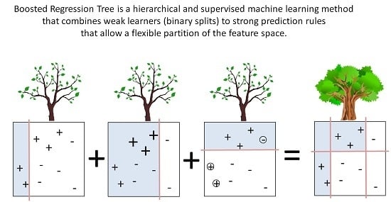
In this paper, we use a boosted regression tree (BRT) to link the response variable (FCover) to the two covariates, namely latitude and longitude of the centroid of the area. A BRT is a popular statistical and supervised machine learning approach that has been readily applied to remotely sensed data. Indeed, although they were first defined two decades ago, BRTs have only recently been extended to deal with the types of features that are characteristic of remotely sensed data, in particular, its spatial and temporal dynamics. BRTs combine two algorithms (regression trees and boosting) and arguably yield higher prediction accuracy than simple tree-based methods such as a Classification and Regression Trees (CART) [30]. There are two major advantages of using BRT over more traditional regression methods. First, it allows a more flexible partition of the feature space that is not as rigid as using a simple linear regression. BRT combines simple binary partitions to form a complex prediction rule that can more accurately identify small areas of interest. Second, it can deal with missing values by default, such as masked out areas (clouds and cloud shadows), water bodies or the Scan Line Error of Landsat 7 ETM+. This is a great advantage especially when using remotely sensed imagery that has gone through several quality refinements and processing levels to filter out obscuring elements that leave data gaps behind.
The aggregated fractions of green vegetation derived from the FCover scene serve as our response variable. The delineated centroid coordinates from the midpoint of the spatial grid cells serve as surrogates for other spatial covariates and represent a north-south gradient shown as a vector of latitude coordinates and an east-west gradient shown as a vector of longitude coordinates. These surrogate variables will be used to statistically analyse the relationship to our response variable and the quantitative impact on prediction accuracy of different spatial aggregation schemes.
The use of latitude and longitude as surrogates for other covariates is not uncommon. For example, in a study of the geographic distribution of plant functional types [31] the authors examined the relationship of precipitation and temperature on C3 and C4 grass types and shrubs using latitude and longitude coordinates and concluded that latitude and longitude can be used as surrogate variables for the main climatic dimensions in North America. The latitude and longitude explained a substantial portion of the variability of the distribution of the relative abundance of shrubs, C3 grasses, and C4 grasses. Along a given longitude, C3 grasses increased with latitude. As one moves westward, C4 grasses are replaced by shrubs. In another study [32] the authors plotted latitude and longitude coordinates and included these as surrogate variables to account for variation in climate associated with geographic location within deciduous forested ecoregions. The response was an aggregated NDVI variable used as an on-site quantification of vegetation in North America.
In summary, the objective of our study was to analyse the statistical dependence between our two surrogates, the centroid coordinates in latitude and longitude, and their ability to predict the aggregated fractions of green vegetation delineated from the FCover scene. The focus is on the prediction accuracy achieved in four spatial resolutions and the preprocessing time needed to extract and aggregate the green fractions out of the FCover scene. We use a BRT to link FCover with the two covariates.
The paper is structured as follows. Section 2 presents the data and BRT methodology used for predicting green vegetation using geographic centroid coordinates of evenly spaced spatial grid cells, the relevance of the spatial aggregation measured as a model fit and a brief reminder about the principles of spectral unmixing approaches and its outcome. Section 3 presents the results structured in three groups: (1) the comparison of the model fit showing the distribution of the residuals around the mean, (2) the variable interactions as the relative influence and partial dependencies of the covariates on the response variable, the relationship and distribution of the predicted versus the observed test data set in marginal plots and model diagnostics and (3) the aggregation and scaling errors using different spatial resolutions. The outcome and the relevance of this work to real word scenarios and limitations of BRT are discussed in Section 4.
2. Material and Methods
2.1. Case Study
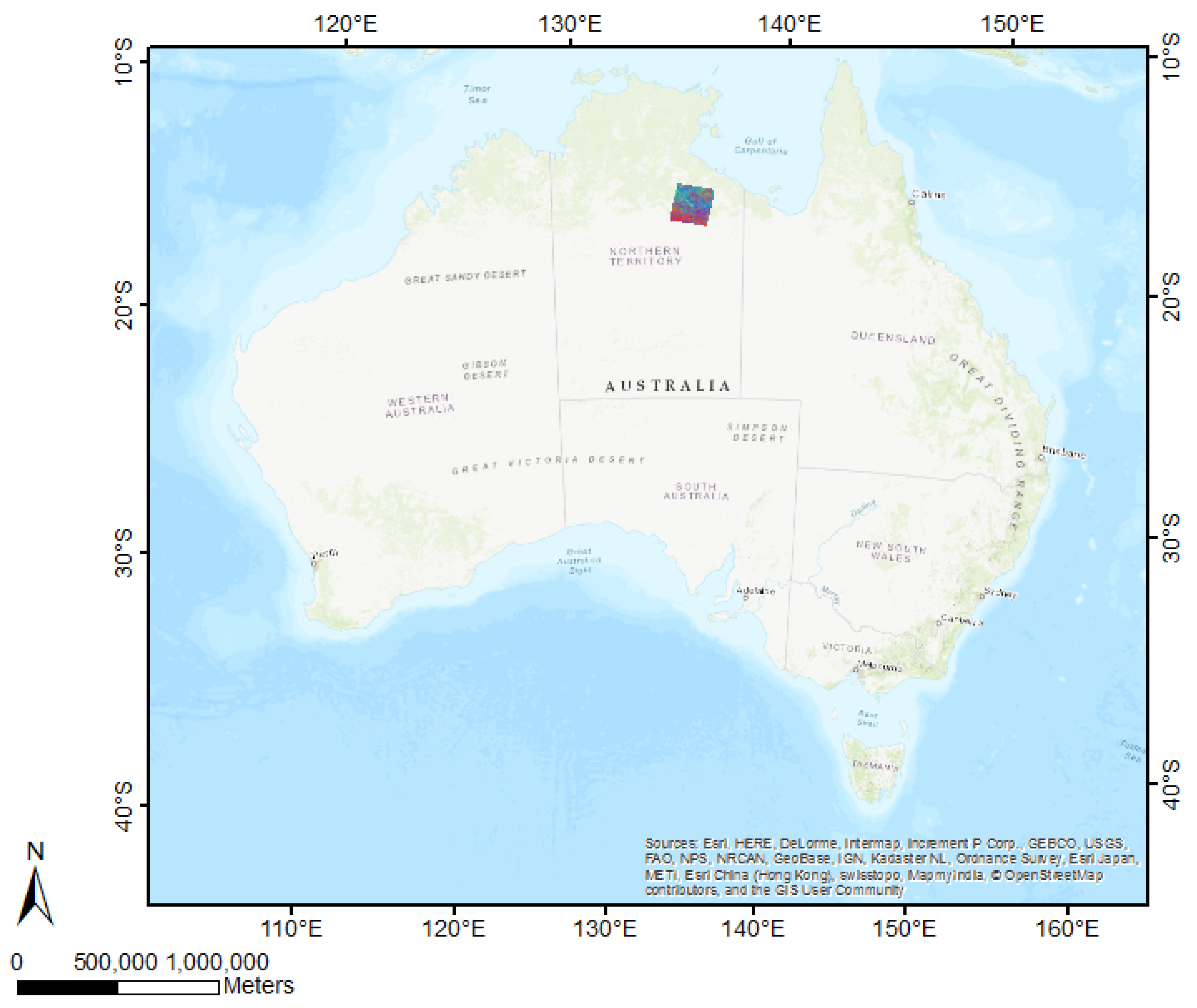
The study area used in our assessment is located in the Northern Territory, Australia. Figure 1 shows the location of the FCover scenes at the Landsat footprint of path 102 row 72 at the Worldwide Reference System-2 (WRS-2) covering an area of 185 × 185 km. The geographic coordinates are given as centroids showing latitude −17.345 and longitude 135.587. For consistency over time, and because the FCover in the study area is dominated by wet and dry seasons, only December scenes indicating the very early period of the wet season have been used for this case study. Estimating FCover at this time of the year is important for agricultural managers. The study area is a heterogeneous region with a complex topography of native grass types.
Our study area is defined as “dry” with variations of “desert, hot arid” and “dry summer, hot arid” (BWh and Bsh) based on the Koeppen-Geiger scheme and is very vulnerable [33,34]. The daily rainfall in December has been recorded as lowest at 16.2 mm in 1990 and highest at 96.4 mm in 1989, and the monthly total ranged from 38.0 mm in 1990 to 137.2 mm in 1987 [34].
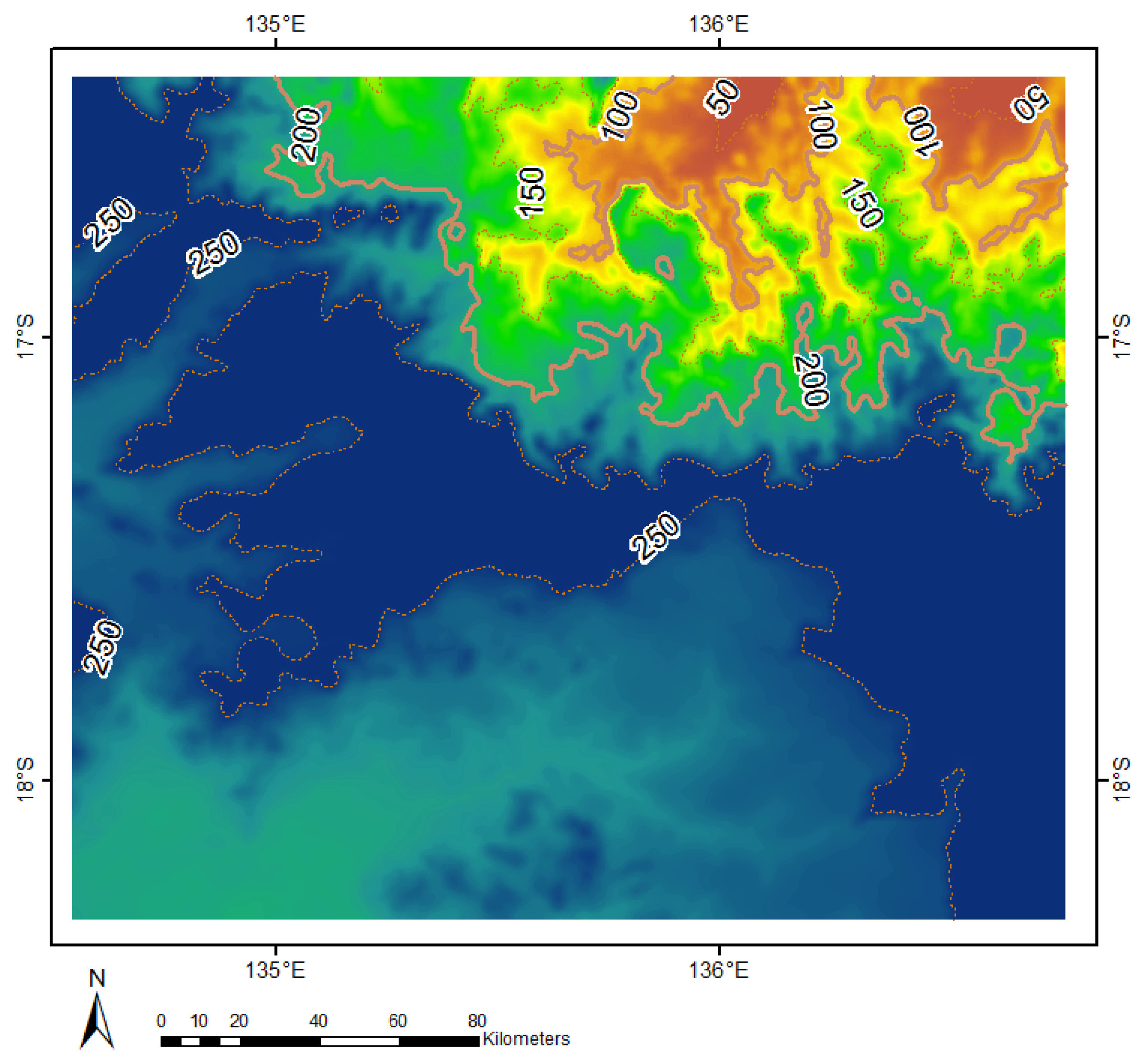
We used a Digital Elevation Model (DEM) and generated equidistant contour lines in 50 m intervals. Two DEMs were merged and clipped together to the full extent of our spatial raster grid. We used the freely available SRTM 90 m resolution and used focal statistics on a 33 × 33 cell neighbourhood to smooth the surface so that the spatial resolution of the DEM represents our aggregated green vegetation fractions better. The highest point is 255 m and the lowest is located at 23 m ( m) above mean sea level (MSL) referenced to the Australian Height Datum (AHD). In Figure 2 we can see a constant increase of about 15% of the elevation between the upper right corner (min 23 m) to the lower left corner (max 255 m).
2.2. Data
Spectral Unmixing Approach
The opening of the Landsat archive and a new open data policy have revolutionised the use of Landsat data [13]. The Fractional Cover product is derived from Geoscience Australia and the Australian Reflectance Grid 25 (ARG25) product and provides fractional cover representation of the proportions of green or photosynthetic vegetation, non-photosynthetic vegetation, and bare surface cover across the Australian continent. It is generated using the algorithm developed by the Joint Remote Sensing Research Program (JRSRP) and described in [19]. FCover is available for Landsat Thematic Mapper (Landsat 5), Enhanced Thematic Mapper (Landsat 7) and Operational Land Imager (Landsat 8). FCover was made possible by new scientific and technical capabilities, the collaborative framework established by the Terrestrial Ecosystem Research Network (TERN) through the National Collaborative Research Infrastructure Strategy (NCRIS), and the leadership and capabilities of Geoscience Australia and the Joint Remote Sensing Research Program [35].
The spectral unmixing approach aims to separate the spectral reflectance of one pixel into its single ground cover components to determine the proportions of each of three classes PV, nPV and BS. The result of spectral unmixing is a series of three layers showing the fraction of each abundance images corresponding to each class and an image depicting the root mean square error (RMSE). Our FCover scene is located in the Northern Territory where the land is mainly used for grazing. It is rare to find a pure pixel in heterogeneous grazing land [19]. Further information about how the field data collection has been conducted and how to derive spectral endmembers using spectral unmixing approaches is provided in [36].
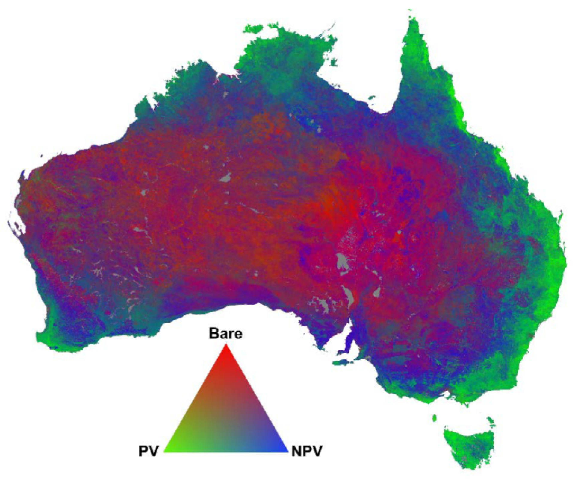
Figure 3 shows a national FCover product for Australia. The triangular ternary diagram can be read anti-clockwise between PV, nPV and BS. The interpretation of the colour coded fractions is based on the additive colour coding principle showing the relationship between the three endmembers. A quantitative Attribute Accuracy Assessment of the spectral unmixing approach and the overall error of the fractional ground cover RMSE is 11.8%, while the error margins vary for the three different layers where green vegetation has an RMSE of 11.0%, non-green vegetation 17.4%, and bare soil 12.5%. The validated Landsat derived fractional cover products are now used as key indicators for a range of environmental monitoring and management activities [22].
2.3. Data Exploration for FCover Imagery
A FCover scene consists of three layers showing the fractions of each ground cover class in each layer. As part of our explanatory data analysis, we plotted histograms for all four years of the study period to review the distributions of PV, nPV and BS. Figure 4 shows the ground cover classes of the Landsat FCover bands combined in one histogram, along with the frequencies. We can clearly see that green vegetation has the least fractions but a high frequency, whereas non-green vegetation has higher fractions presented in one pixel.
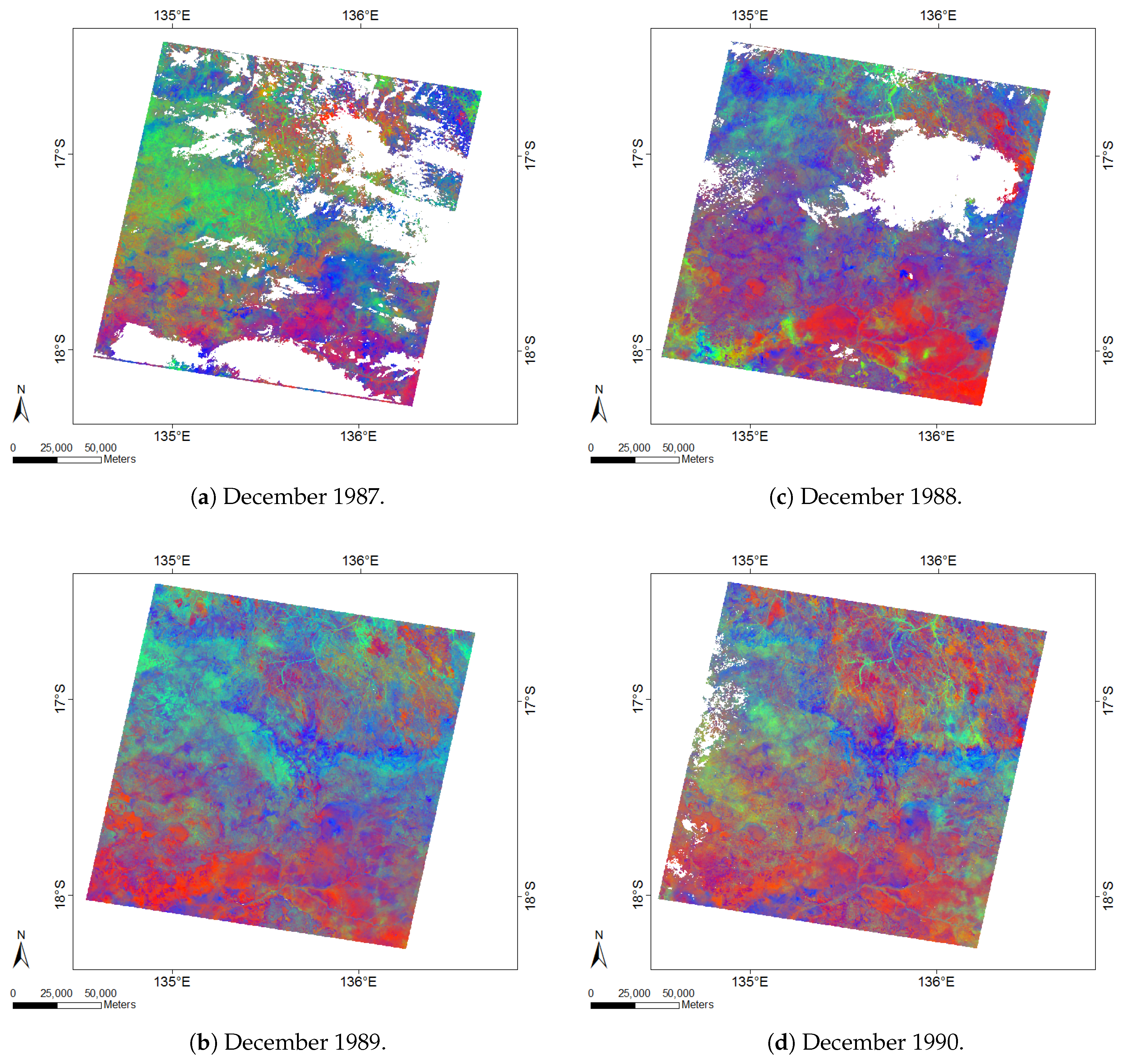
The histograms indicated a roughly normal distribution for each of the classes. It can be seen that the green vegetation has the smallest fractions. In 1988, 1989 and 1990 the green vegetation was represented as the smallest fraction but with the highest frequency, except in 1987 where the bare soil has the lowest percentages and the mode (represented as the highest bar) of the green vegetation shifts towards 20% and higher. This is an indicator that in 1987 the PV is more strongly represented than in the rest of the three years and therefore, we can infer that December 1987 was our wettest month. This is in accordance with the recorded rainfall data, described in the case study, where the monthly total is the highest in all of our FCover scenes. Moreover, the mode of green vegetation is smallest (around 12.5%) in 1990 and this reflects the lowest recorded monthly total and the lowest recorded daily rainfall in December 1990 as described earlier. Hence, 1990 is described as our driest year [34]. Figure 5 shows the four FCover scenes and their masked out areas.
2.4. Data Pre-Processing and Spatial Aggregation
The aggregation involved several pre-processing steps. As one of the pre-processing steps, we created four evenly spaced spatial grid cell layers in four different spatial resolutions, showing the same geographic reference as the FCovers scenes and overlaid this on the raster image. The spatial grid layers were used as a vector overlay on the FCover scene showing varying coarseness of the grid cells extents ranging from the spatial resolution of 12,000 m, 6000 m, 3000 m and 1500 m. In addition, we ensured that the edges of the spatial grids lined up with the edges of the FCover pixels. Further, all missing values were removed and the arithmetic mean was calculated for each spatial grid cell. Figure 6 shows the spatial grid on top of the FCover scene at a resolution of 3,000 m. The figure also shows the extent of missing data, due to masking out obscuring elements such as cloud and cloud shadow.
The spatial resolution determines the geographic extent of each spatial grid cell in the FCover scene. One spatial grid cell in 12,000 m contained 400 × 400 FCover pixels each having a geographic resolution of 30 × 30 m and covering a total area of 12,000 × 12,000 m on the ground (400 × 30 m = 12,000 m). In contrast, the spatial grid resolution of 1500 m contains 50 × 50 pixels and covers an area of 1500 × 1500 m within the spatial grid cell. Table 1 lists all the spatial resolutions used in this study, the number of pixels contained within a spatial grid cell as an overlay on the FCover scene, the total area covered on the ground and the total number of spatial grid cells in the overlay used for the proposed aggregation scheme. The choice of the spatial resolutions allows for consistent arithmetic averages of FCover to be taken over the aggregated cells.
The four spatial grids demonstrated in Figure 7 were obtained using the open source software GME (Geospatial Modelling Environment). GME currently has dependencies on ArcGIS and R where it uses the statistical engine to drive some of the analysis tools.
Each individual grid cell was used to calculate the arithmetic mean as a measure of central tendency of all the pixels contained within the spatial grid cell extent. As a result, one aggregated value of all green vegetation fractions contained within the grid cell extent represented each individual grid cell with the aggregated PV fraction. Since the spatial grid cells line up with the edges of the FCover pixels, adjacent and overlapping pixels will not be considered in the aggregation process.
In addition to aggregating fractions of green vegetation spatial grid cells sizes we delineated the centroid coordinates as geographic latitude and longitude coordinates of each grid cell. The resultant csv file contained the response variable of aggregated fractions of green vegetation and the centroid coordinates in latitude (North-South direction) and in longitude (East-West direction). As discussed in the Introduction, no additional environmental data were used for the following modelling process using BRT. Altogether 16 csv files were created representing four spatial aggregations scheme for four years. Table 2 shows further details.
2.5. Boosted Regression Trees
A boosted regression tree (BRT), also known as gradient boosted machine (GBM) or stochastic gradient boosting (SGB), is a non-parametric regression technique that combines a regression tree with a boosting algorithm [37] (Appendix A.1). This extension to the classical regression tree allows greater flexibility and predictive performance in modelling the data. The implementation of these methods used in this study can be found in the gbm R package [38].
A regression tree partitions multivariate data with a hierarchy of binary splits that define regions of the covariate space in which the response variable has similar values. These splits are defined by rules, distance metrics or information gain. The choice of variables and the value at which the split point occurs are determined in a recursive manner at each stage of the tree construction. The segmentation can be depicted as a tree-like structure, comprising nodes representing the selected factors, branches acting as if-else connectors between the nodes, and leaves representing terminal nodes containing the subsets of responses [39,40,41].
The performance of the simple base learner is improved by boosting, whereby a sequence of trees is grown, such that in each subsequent tree greater attention is paid to observations with greater prediction error. This is achieved by iteratively shifting the focus towards those observations until a stopping rule is reached. The shift is effected by up-weighting observations that were misclassified or had large residual errors in the previous iteration. The deeper tree accommodates more segments and hence captures more variance. This results in higher model complexity but also higher risk of overfitting the model to the data. The motivation behind boosting is that each tree can be quite shallow (a weak classifier) and thus fast to estimate, but by combining the predictive power of many weak classifiers, a classifier of arbitrary accuracy and precision can be created [42,43,44].
Next, the current approximation is individually updated in all of the corresponding regions
The shrinkage parameter, , ranges from 0 to 1 and controls the learning rate , so each gradient step is reduced by some factor between 0 and 1 of the learning rate. The value of is influenced by the choice of loss function .
| Algorithm 1 Stochastic Gradient Boosting algorithm. |
|
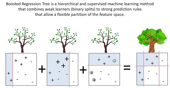
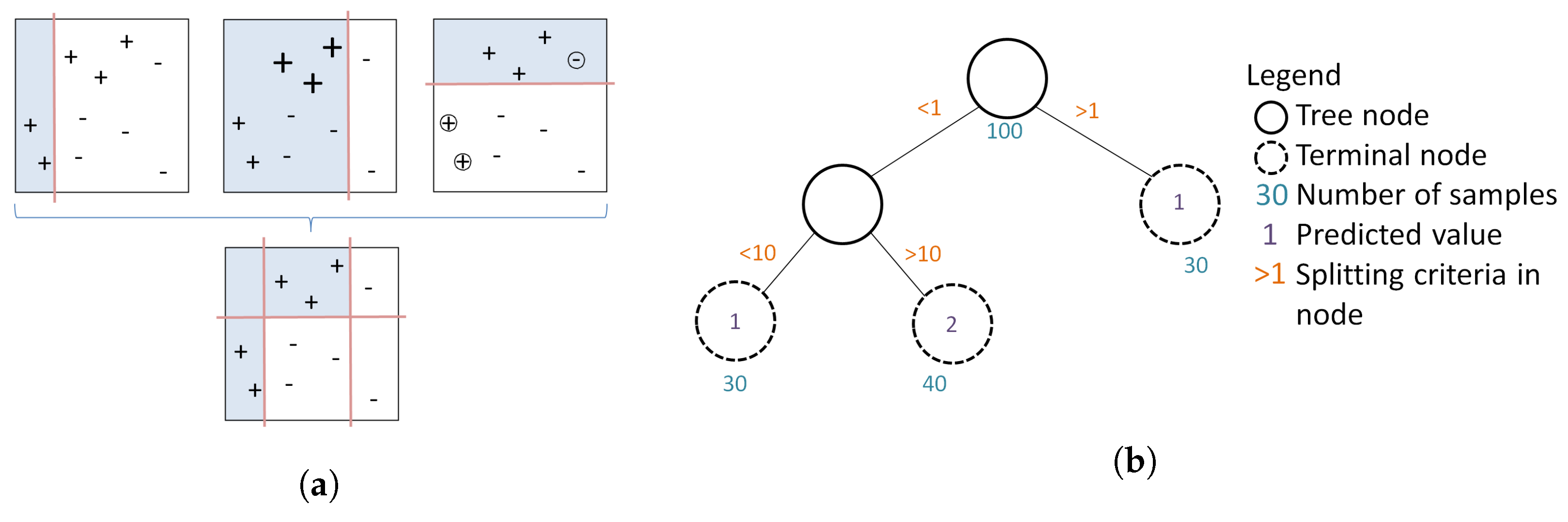
Figure 8a shows four splits of the whole feature space of the data where the goal is to predict the plus symbols (+). The first three are binary splits that will be combined into one complex splitting rule (bottom). This yields a more accurate prediction result by separating the data allowing for flexible splitting boundaries. The first binary split (left) shown as the red vertical line has incorrectly predicted three observations indicated with a plus symbol. The misclassified observations get a higher weight to make sure those are favoured in the next splitting iteration (middle). The plot in the middle shows that three observations indicated with a minus symbol (−) are now misclassified. In the following step those misclassified observations will get higher weights again to be prioritised not to be included in the next splitting process. This time a horizontal line is generated. BRT is an ensemble approach and combines the first three binary splits above into one in order to create a complex prediction rule to split data allowing for identification of small areas of interests. This is the boosting part of BRT.
2.6. Implementation
The R package caret [47] was used for two tasks. The first was to split the data into training and test datasets (random partition that assigns 80% of the data in a training set and the remaining 20% to a test set) and the second task was to tune the hyperparameters for BRT modelling.
Typical hyperparameters include the
- shrinkage; (how quickly the algorithm adapts)
- tree complexity; the total number of trees in the final model (number of iterations)
- interaction depth; interaction between different nodes along the branch
- minimum observations in node; minimum number of training set samples in a node to commence splitting.
A feature of the BRT algorithm is that the performance can be tuned to accommodate specific data structures and characteristics through specification of hyperparameters. For our BRT model, the carat package was employed to find optimal values for the hyperparameters listed above. We used the automatic grid search method for searching optimal parameters, combined with other methods for estimating the performance of our gbm model based on our aggregated FCover data.
The outcome of the tuning process for all the 16 models was a recommendation of number of trees = 2500, interaction depth = 5, (only data of 1987 in 12,000 m recommended 3), shrinkage = 0.01, and minimum observations in node = 10. Those hyperparameters were then used to estimate the coefficients using the training data, and the prediction results are based on the test data set. Cross-Validation methods were used for the tuning process to help identify the hyperparameters and to restrict the number of iterations (hyperparameter tree complexity) to avoid overfitting when the local minimum has been reached. Empirically, it has been found that using a small value for shrinkage results in impressive improvements in a model’s generalisation ability [45]. The drawback of a lower learning rate is that more trees need to be generated, resulting in increased computational time. As described above, altogether 16 BRT models were created showing four years in four spatial resolutions; see Table 1.
2.7. Quantitative Assessment of the Model Fit
The accuracy of the 16 BRT models was primarily analysed on the basis of the root mean square error (RMSE), the mean absolute error (MAE) and the median absolute error (MDAE), where we measured the difference between values predicted by a model and the values actually observed from the environment that is being modelled on the test dataset. In general, the RMSE is best when it is small, but there is no absolute good or bad threshold. The RMSE ranging between 3.3 and 1.1 indicates a good model fit throughout all resolutions.
3. Results
The computational environment was the R statistical modelling software version 3.3.3 [48] running inside Windows 7 SP1 (64-bit) on a 2.60 GHz Intel i7 CPU with 16 GB of RAM. All of the plots were generated in the R programming language [48] and maps throughout this paper were created using ArcGIS® software by Esri. The GBM model implementations were taken from the gbm package [38]. We structure our results in three main groups. Since we want to investigate prediction accuracy using different spatial aggregations we first checked the residuals and how they spread around the mean of the regression line and the model fit in all the 16 models. Second, we evaluated the influence of each covariate on the response, shown by relative influence plots, or the functional relationships between the covariates and the prediction outcome indicated by partial dependency plots (Appendix A.2). Further, we investigated the relationship and distribution of the observed versus the predicted values in marginal plots. Last, we visualised the absolute error rate depending on the spatial resolution in all years and compared those with the elapsed time.
3.1. Comparison of Model Fit at Different Spatial Resolutions
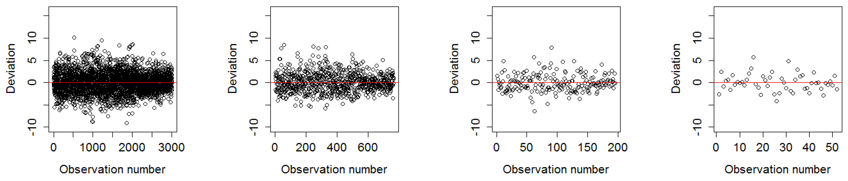
3.1.1. Deviation of Residuals Around the Mean
Summary statistics and plots revealed that the residuals of the fitted models were relatively unbiased and homoscedastic. The residual plot of the worst model fit of the year 1988 in 1500 m and 12,000 m showed a slight tendency to heteroscedasticity due to a larger variance of the fitted values towards the maximum number of observations and further the resolution 12,000 m showed an unbalanced spread around the regression line towards under-predicted values shown in Figure 9. These effects were not visible in any of the residual plots for the best model fit in the year 1990 demonstrated in Figure 10.
Figure 11 shows the combined residuals over all years for all resolutions on the left and the corresponding box plots on the right.
The box plots show that the deviation of the residuals within the Inter Quartile Range (IQR), indicated as the white box around the zero line, is similar regardless of the spatial aggregation. However, there is more variation in the resolution of 1500 m than in any other resolutions. This can be explained by the argument that the loss function used in the BRT and the weighting of problematic observations result in a similar deviation of the residuals at all aggregated spatial resolutions.
We can see that the 6000 m resolution has the least error rates and is most symmetrically distributed around the black line showing the mean of the residuals. We conclude that aggregating from an initial geographic resolution of 30 × 30 m to 6000 m resolution resulting in the largest reduction in data volume without sacrificing precision of the prediction.
Table 3 shows the RMSE error rates for the four resolutions and four years. In general the smaller the RMSE error, the better the model fit.
3.1.2. RMSE Comparisons between BRT and Linear Model (LM)
To evaluate the comparative performance of the BRT results, the data were also analysed using a linear regression model. The R package lm.br [49] was used to fit the model. We assume that green vegetation, denoted as , is linearly related to the covariates latitude and longitude, denoted as and respectively, and the residuals are distributed . The LM was formulated as follows:
The comparative goodness of fit of the LM and the BRT is shown in Table 4. It is clear that under all four spatial resolutions, the BRT delivers a smaller RMSE. Based on this measure of performance, the BRT is argued to be an attractive alternative to the more common LM approach for analysing these types of data.
3.1.3. Mean Absolute Error (MAE) and Median Absolute Error (MDAE)
In addition to the RMSE, we calculated the mean absolute error (MAE) and the median absolute error (MDAE) shown in Table 5. MAE computes the average absolute difference between observed and predicted values as the vertical or horizontal distance between each point in a scatter plot. MDAE computes the median absolute difference between the two values. Please see Table 5 for details. In Section 3.2.4, we see in the marginal plots that BRT under-predicts peak values. In Section 3.3 we use the absolute error to quantitatively assess the difference between observed and predicted values for all four spatial resolutions and all four years.
3.2. Variable Importance
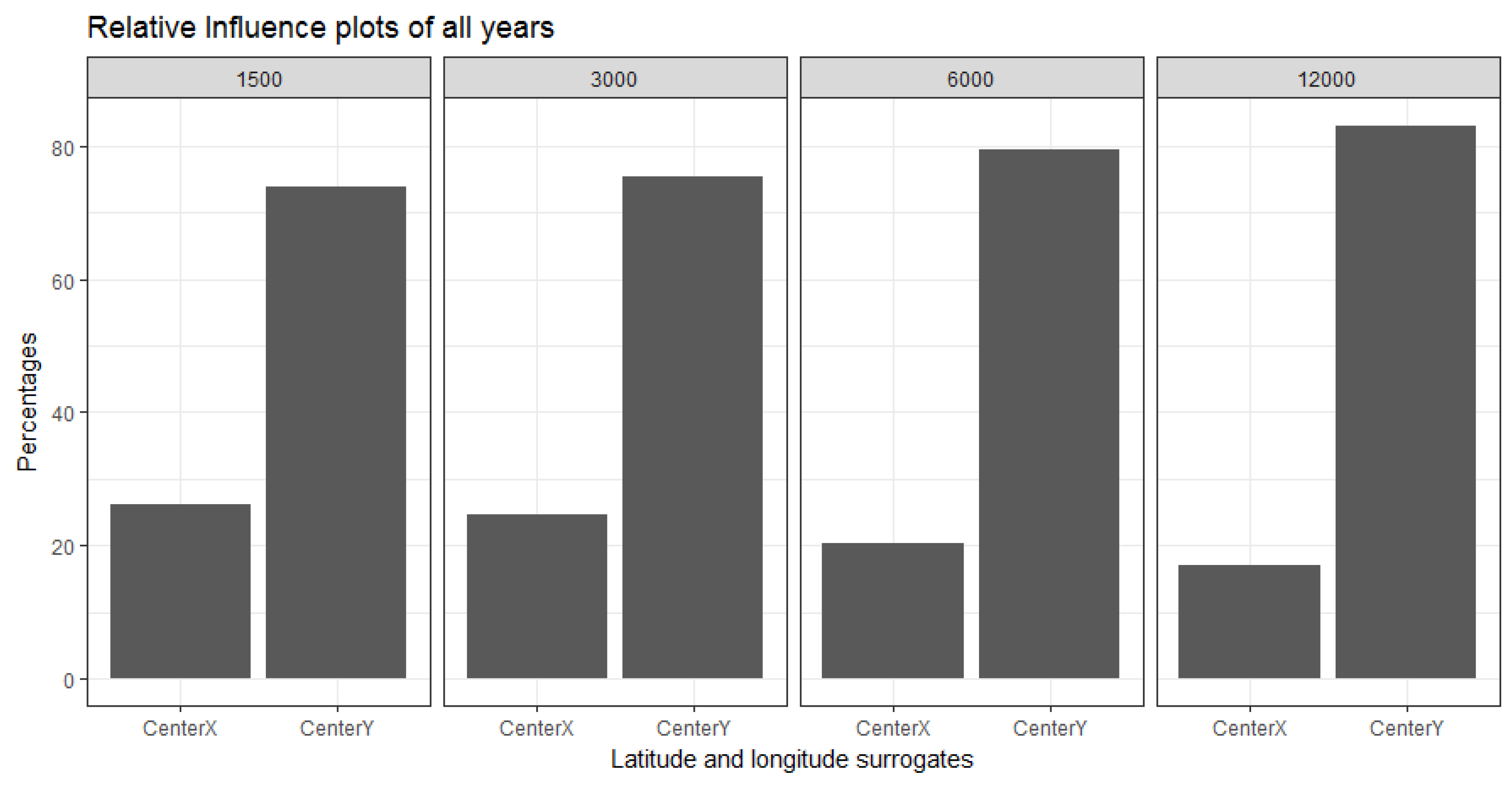
3.2.1. Relative Influence of Covariates at Different Resolutions
One way of showing the relationships of the joint probability and contribution of our geographic coordinates in describing the response is through a relative influence plot. The relative influence is calculated by averaging the number of times a covariate is used in the tree building process, weighted by the squared improvement to the model as the result of each split. It is then scaled so the values sum to 100 [50]. Relative influence plots were used to compare the covariates with respect to their explanatory power. Regardless of the spatial resolution, among the two covariates used in the BRT model, the latitude (CenterY) is always more dominant than the longitude (CenterX). Moreover, the influence of the longitude (East/West direction) reduces as the spatial resolution is decreased towards 12,000 m. However, this is not a consistent reduction. In Figure 12 we demonstrate the influence of CenterX and CenterY covariates and their contribution towards predicting the aggregated green vegetation in the year 1989. The plots show the contribution at the best-estimated number of trees of 2500 iterations starting at 73.91% in 1500 m and reaching the maximal influence of 83.15% in 12,000 m. The relative influence of latitude (CenterY) dominates considerably over longitude (CenterX).
3.2.2. Prediction Raster Maps
The Prediction Raster Maps clearly demonstrate a change in the marginal effect across spatial resolutions, seen as a smoothing effect towards the 12,000 m resolution; see Figure 13.
3.2.3. Prediction Surface Plots
As fractional cover varies with the geographic coordinates, the partial dependence can be shown as a prediction surface plot. Here, the independent variables CenterX and CenterY are plotted against the model outcome after considering the average effect of the other independent variable in the model. Since, we only have geographic coordinates as covariates we get a prediction surface plot showing the comparative influence of the latitude and the longitude as seen in Figure 14.
3.2.4. Marginal Influence Plots
Marginal plots help in understanding the interaction effects of two variables by displaying the marginal relationship between the predicted aggregated fractions and the observed values of the test data set. Marginal plots also provide useful diagnostic information about the fitted model.
Figure 15 shows the marginal plots for the best model fit in the year 1990. The plots indicate that the BRT model under-predicts high observed values throughout all resolutions. This is especially apparent in the longer tails of the right-skewed histogram and density curves shown on the observed axis. In general, all plots exhibit a positive and relatively strong relationship, with a tendency towards clustering at the predicted values as seen by the vertical multi-modal histogram and density plot on the predicted axis. This is especially true in the resolution of 12,000 m where three clusters are evident, whereas in the resolution of 1500 m it seems there is more smoothing present. This is a feature of the BRT design, as described in Section 2.5.
3.3. Aggregation and Scaling Error
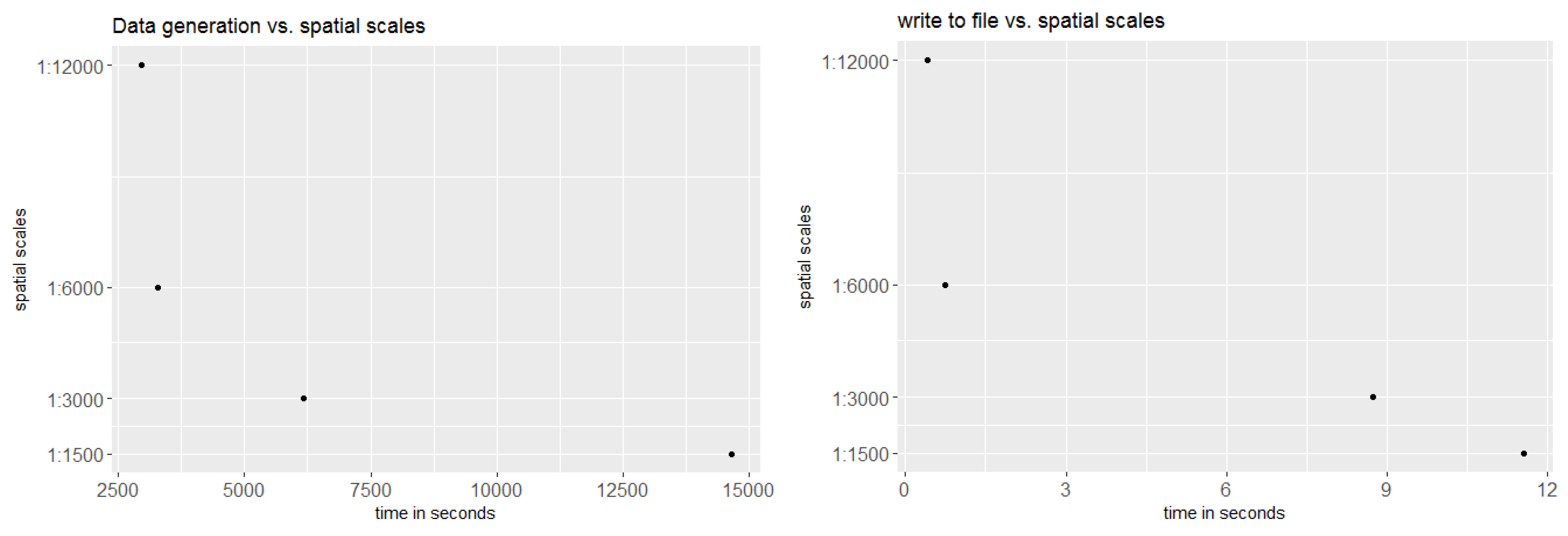
We investigated the effect of spatial aggregation on prediction accuracy and compared the predictive outcome to the computational time to delineate aggregated means out of the FCover band for green vegetation. We argue that a full FCover scene is not required in order to achieve satisfying prediction results and therefore investigated finding a threshold of a spatial resolution that yields acceptable results but is also computationally inexpensive. For this, we recorded the elapsed time to generate the mean of the spatial grid cells and the time required to write the calculated mean to a csv file.
Figure 16 provides comparative information about computational time for the different spatial resolutions. The dominant factor in computing time was delineating the aggregated means from the FCover band for PV.
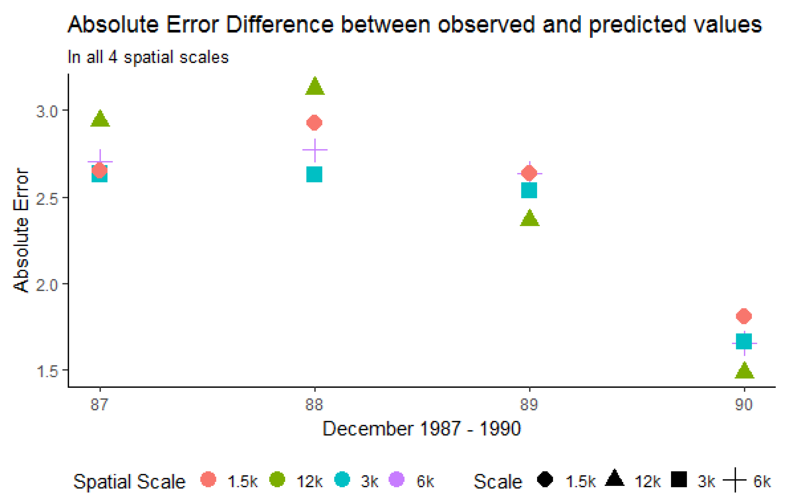
The effect of the four aggregation resolutions on the prediction accuracy is depicted in Figure 17. For this plot, we calculated the absolute difference between the observed and the predicted values for all the years present in this case study. The largest and smallest error rates were observed at the resolution of 12,000 m, whereas the resolutions of 3000 m and 6000 m showed the most stable performance. It should be noted that the resolution of 1500 m also yielded lower absolute error rates, but there was a trend towards higher rates in 1988 and 1990. Overall, the 3000 m resolution showed the best error rates, followed by 6000 m. These resolutions also have a reasonable processing time as shown in Figure 16.
The overall conclusion based on the inspection of the times is that the resolution of 3000 m is best, followed by 6000 m with regards of processing time, prediction accuracy, the strong and positive interaction effect shown in the marginal plots and a significant relative influence of the contribution of CenterY in the splitting process of min 52% and max 75%.
4. Discussion
The goal of this paper was to investigate how spatial aggregation affects prediction accuracy of green vegetation using a BRT model. We focused our evaluation on a case study and chose four aggregation schemes that follow a linear scale. Aggregating the fractions of green vegetation and calculating the mean does alter the original fractions of PV. This alteration can be seen as the consequence of data compression. In our case, we introduced a compression that causes loss since the original fractions cannot be recovered by decompression. The results show that it is not necessary to compute FCover at full (30 m) spatial resolution to obtain satisfactory predictions. This is an important outcome since the computational time will be significantly reduced by spatially aggregating the fractions of the FCover scene. Figure 16 shows the reduction of time needed for the data generation process in extracting the means. This is especially important when more than one FCover scene is used. However, comparisons between aggregations are not straightforward, particularly because the data quality (showing large data gaps) and green vegetation cover differs between the scenes. Further investigation is still necessary to test BRT on homogeneous land to assess whether the best spatial aggregation resolution identified here as 6000 m is still the same and whether the prediction accuracy is affected by a different topography. We demonstrated that the BRT outperformed the LM by achieving much better RMSE rates.
In this paper, we first demonstrated that the distribution of residuals around the mean is relatively consistent throughout the resolutions. Moreover, in our study latitude and longitude coordinates alone were shown to be able to effectively predict FCover. We showed the strong relationship between latitude and longitude in the marginal plots in Figure 15.
In the relative influence plots we demonstrated that the centroid of the latitudes (indicating North-South direction) are far more dominant in describing the aggregated FCover mean values. For reasons discussed in Section 2.2 it is not surprising that the latitude dominates over longitude with regard to green vegetation. What is surprising though is the high contribution and very strong influence of around 80% as shown in Figure 12.
The marginal plots illustrate that BRT under-predicts high peak values throughout all resolutions. We argue that 72 FCover mean values of 12,000 m can represent the existing green vegetation in one scene. Further, we could demonstrate that the scene offered enough heterogeneous land cover and the Landsat footprint of 185 × 185 km was sufficient to show the targeted and generalisable results.
Another interesting investigation would be to use multi-sensory imagery and multi-granularity pixel sizes as additional covariates in the modelling process. We focused on the exact alignment of pixel edges to the spatial grid by choosing a resolution that incorporates full pixels. However, before we used the resolutions here, we had more common ones in 1000 m, 5000 m and 10,000 m and the data extraction time was significantly increased due to the effect of incorporating adjacent pixels that overlapped with the spatial grid cell.
Limitations of our approach can be found in the aggregation scheme using the arithmetic mean. When extracting the mean of a spatial grid cell we do not know the distribution of fractions within the grid cell since we only obtain one value representing the aggregated fractions. Different methods of aggregating values may provide better capture of cell statistics and data structure within a spatial grid cell.
An alternative way of using FCover fractions is to sum all the vegetation (nVP and VP) and compare those values with the fraction of bare soil in a presence/absence study. This could be useful in time series analysis, such as an investigation of an increase or decrease of vegetation versus bare soil. This is of particular interest with ongoing climate change towards desertification in arid or semi-arid areas. A potential approach is to use indicator functions that can encode logical and simple calculations by defining thresholds in order to investigate if fractions of the combined vegetation versus bare soil represent values greater than the set threshold of both classes. Depending on the magnitude of a fraction, the pixel could be mapped to categorical values used in the modelling process instead of our approach of using continuous values. BRT can deal with continuous and categorical response values.
There are many features of BRT that are advantageous for the problem considered here. The BRT model itself comprises a flexible regression structure with improved predictive performance effected through boosting. Boosting is an adaptive method for combining many simple models to give an improved predictive performance. In addition to the computational speed and accuracy of estimation, they can describe complex non-linearities and interactions between variables, accommodate missing data, include different types of input variables without the need for transformations or elimination of outliers, perform well in high-dimensional problems, and allow for different loss functions such as accurate identification of small areas of interest. Moreover, they can be visualised and interpreted easily, thus facilitating the translation of the analytic results to decision makers [44]. The predictive accuracy of BRT has been investigated both theoretically [42,43] and in various applications [51]. Although BRT models are complex, they can be summarized in ways that give powerful ecological insight, and their predictive performance is superior to most traditional modelling methods.
To sum up, BRT is a very flexible, statistical and hierarchical machine learning approach that can be used in various remote sensing aspects. In a study by Kotta [52] the author combined hyperspectral remote sensing and BRT to test their ability to predict macrophyte and invertebrate species cover in the optically complex seawater of the Baltic Sea and concluded that there is a strong potential for BRT in modelling aquatic species. Further, Jafari et al. [5] evaluated the suitability and performance of BRT for soil mapping using a limited point dataset in an arid region of Iran. The performance was tested in two scenarios: (i) using only the DEM and remote sensing covariates and (ii) additionally using the geomorphology map. Results showed that the geomorphology map contributed importantly to the prediction accuracy. In addition, Colin et al. [50] combined a collection of GIS shapefiles, remotely sensed imagery, and aggregated and interpolated spatio-temporal information to one input file that resulted in a structured but noisy input file, showing inconsistencies and redundancies. It was shown that BRT can process different data granularities, heterogeneous data and missingness. A comparison with two similar regression models (Random Forests and Least Absolute Shrinkage and Selection Operator, LASSO) showed that BRT outperforms these in this instance. Last but not least, Pittman [53] investigated coral reef ecosystems that are topographically complex environments and possess structural heterogeneity that influences the distribution, abundance and behaviour of marine organisms. They used BRT and LIDAR data that provided high resolution digital bathymetry from which the topographic complexity was quantified at seven spatial resolutions of 4, 15, 25, 50, 100, 200 and 300 m [53]. They concluded that the combination of BRT and LIDAR has a great utility in the future development of benthic habitat maps and faunal distribution maps to support ecosystem-based management and marine spatial planning.
5. Conclusions
A data reduction scheme on FCover showing only the green vegetation fractions, and using BRT to assess the influence of the data reduction on the predictive power of BRT is proposed in this paper. The first step of the proposed method aims to reduce the heterogeneous green vegetation cover through aggregation based on an evenly spatial grid that served as an overlay for the delineation of the green vegetation fractions. This was performed at four spatial resolutions of 1500 m, 3000 m, 6000 m and 12,000 m and resulted in 16 input files for the BRT modelling approach. The files were split into training and test set and BRT was then applied to identify the influence of the spatial resolution on prediction accuracy for BRT models. To validate the performance of the proposed method, the RMSE, MAE and MDAE were considered. Further, the predictive performance of the BRT was compared with that of the more common linear regression model and was found to consistently deliver smaller RMSE values at all four spatial aggregations. The analysis showed that the proposed method can also provide useful visual interpretations by showing, for example, the prediction raster map and the smoothing factor for each spatial resolution. Based on these results, we conclude that boosted regression trees are an appealing method for estimating green vegetation from remotely sensed images and that an appropriate aggregation scale can be identified that balances computational demand with acceptable loss of predictive accuracy.
Author Contributions
B.C. and K.M. conceived and designed this study; B.C. performed the experiments and wrote the paper; K.M., M.S., S.C. and A.W. analysed the experimental results and edited on the manuscript.
Funding
This research received no external funding.
Acknowledgments
This study was supported by the Australian Research Council (Grant No.:FL150100150) and did not received other external funding. The authors wish to thank (i) Department of Environment and Science (DES) for providing the Fractional Cover data, (ii) Brodie Lawson for helpful comments on the predictive performance of BRT on peak observations, (iii) QUT ACEMS for providing office space and infrastructure to achieve this article and (iiii) the Reviewers and the Editors for their constructive comments and helpful suggestions, which have greatly improved this article.
Conflicts of Interest
The authors declare no conflict of interest.
Appendix A.
Appendix A.1. Mathematical Explanation of the BRT Method
Here, we summarise the method, following Friedman [37]. Consider a response variable y and a vector of predictor variables that are connected via a joint probability distribution . Using a training sample of known values of and corresponding values of y, the goal is to find an approximation to a function that minimises the expected value of a loss function . Boosting approximates by an additive expansion. The parameters and the expansion coefficients are jointly fit to the training data. This is done in a forward stage wise manner. Gradient Boosting [37] approximately solves differentiable loss functions with a two step procedure. First, the function is fit by least squares to the current pseudo-residuals which represent the residuals from the given stage of the tree building.
Then, given , the optimal value of the coefficient is calculated via
Thus, at each iteration m, the tree partitions the feature space into L disjoint regions and predicts a constant value, , in each region. Gradient Boosting proceeds in this way until the base learner is an L terminal node regression tree.
The parameters of the estimated tree are the splitting variables and corresponding split points that define the tree, and this defines the corresponding regions of the partition at each iteration. These are accomplished in a hierarchical top-down approach using a least squares splitting measure [37]. Equation (A1) can be solved individually within each region, defined by the corresponding terminal node l of the mth tree. Because the tree predicts a constant value within each region, , the solution to Equation (A1) reduces to a simple location estimate based on the criterion
First, we initialize the model. To minimize the square error we initialise with the mean of the training set that is defined through and the learning rate . At the beginning of the algorithm we specify the number of trees/iterations shown as m in the for-loop control structure. Friedman [37] added a stochastic element by proposing to draw a random subsample from the full training data set without replacement. This subsample is then used to fit the base learners and compute the model update for the current iteration. The random subsample of size is given by . Adding randomness to the algorithm in this way has been shown to improve the performance of gradient boosting [44]. In the last step of the algorithm the current approximation of is updated in each corresponding region .
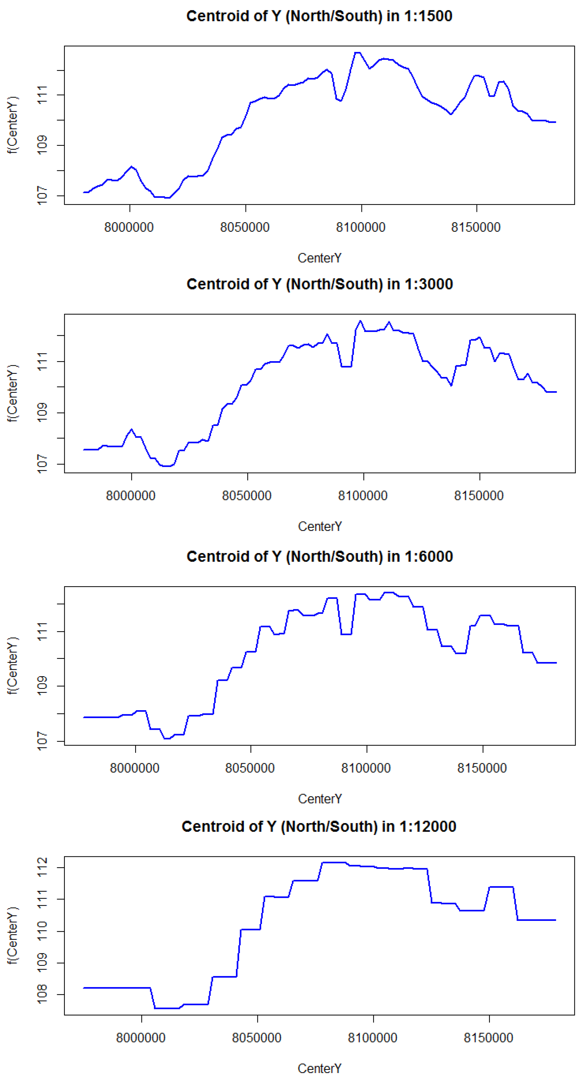
Appendix A.2. Partial Dependency Plots
Partial dependency plots (PDP) are graphical visualizations of the marginal effect of a given variable (or multiple variables) on an prediction outcome.
Figure A1.
Partial dependency plots in 1500 m to 12,000 m from top to bottom of best year 1990. The effect of latitude (CenterY) show similar patterns for the resolution of 3000 m and 6000 m, with a steep linear increase in FCover after a threshold latitude.
Figure A1.
Partial dependency plots in 1500 m to 12,000 m from top to bottom of best year 1990. The effect of latitude (CenterY) show similar patterns for the resolution of 3000 m and 6000 m, with a steep linear increase in FCover after a threshold latitude.

References
- Datt, B. A New Reflectance Index for Remote Sensing of Chlorophyll Content in Higher Plants: Tests using Eucalyptus Leaves. J. Plant Physiol. 1999, 154, 30–36. [Google Scholar] [CrossRef]
- Schmidt, M.; Thamm, H.-P.; Menz, G.; Bénes, T. (Eds.) Long term vegetation change detection in an and environment using LANDSAT data. In Geoinformation for European–Wide Integration; Millpress: Rotterdam, The Netherlands, 2003; pp. 145–154. [Google Scholar]
- Marsett, R.C.; Qi, J.; Heilman, P.; Biedenbender, S.H.; Watson, M.C.; Amer, S.; Weltz, M.; Goodrich, D.; Marsett, R. Remote Sensing for Grassland Management in the Arid Southwest. Rangel. Ecol. Manag. 2006, 59, 530–540. [Google Scholar] [CrossRef] [Green Version]
- Huete, A.; Ponce-Campos, G.; Zhang, Y.; Restrepo-Coupe, N.; Ma, X.; Susan Moran, M. Monitoring Photosynthesis From Space. In Land Resources Monitoring, Modeling, and Mapping with Remote Sensing; CRC Press: Boca Raton, FL, USA, 2015; pp. 3–22. [Google Scholar]
- Jafari, A.; Khademi, H.; Finke, P.A.; Van de Wauw, J.; Ayoubi, S. Spatial prediction of soil great groups by boosted regression trees using a limited point dataset in an arid region, southeastern Iran. Geoderma 2014, 232–234, 148–163. [Google Scholar] [CrossRef]
- Anderson, M.C.; Allen, R.G.; Morse, A.; Kustas, W.P. Use of Landsat thermal imagery in monitoring evapotranspiration and managing water resources. Remote Sens. Environ. 2012, 122, 50–65. [Google Scholar] [CrossRef]
- Washington-Allen, R.; Van Niel, T.; Ramsey, R.; West, N. Remote Sensing-Based Piosphere Analysis. GISci. Remote Sens. 2004, 41, 136–154. [Google Scholar] [CrossRef] [Green Version]
- Stohlgren, T.J.; Ma, P.; Kumar, S.; Rocca, M.; Morisette, J.T.; Jarnevich, C.S.; Benson, N. Ensemble habitat mapping of invasive plant species. Risk Anal. 2010, 30, 224–235. [Google Scholar] [CrossRef] [PubMed]
- Lowell, K. A socio-environmental monitoring system for a UNESCO biosphere reserve. Environ. Monit. Assess. 2017, 189, 601. [Google Scholar] [CrossRef] [PubMed]
- Sarker, C.; Alvarez, L.M.; Woodley, A. Integrating Recursive Bayesian Estimation with Support Vector Machine to Map Probability of Flooding from Multispectral Landsat Data. In Proceedings of the 2016 International Conference on Digital Image Computing: Techniques and Applications, DICTA 2016, Gold Coast, Australia, 30 November–2 December 2016. [Google Scholar] [CrossRef]
- Walsh, S.J.; Crawford, T.W.; Welsh, W.F.; Crews-Meyer, K.A. A multiscale analysis of LULC and NDVI variation in Nang Rong district, northeast Thailand. Agric. Ecosyst. Environ. 2001, 85, 47–64. [Google Scholar] [CrossRef]
- Gallo, K.P.; Easterling, D.R.; Peterson, T.C. The Influence of Land Use/Land Cover on Climatological Values of the Diurnal Temperature Range. J. Clim. 1996, 9, 2941–2944. [Google Scholar] [CrossRef] [Green Version]
- Wulder, M.A.; Masek, J.G.; Cohen, W.B.; Loveland, T.R.; Woodcock, C.E. Opening the archive: How free data has enabled the science and monitoring promise of Landsat. Remote Sens. Environ. 2012, 122, 2–10. [Google Scholar] [CrossRef]
- Zhang, H.; Li, Q.Z.; Lei, F.; Du, X.; Wei, J.D. Research on rice acreage estimation in fragmented area based on decomposition of mixed pixels. Remote Sens. Spat. Inf. Sci. 2015, 40, 133. [Google Scholar] [CrossRef]
- Guerschman, J.P.; Scarth, P.F.; McVicar, T.R.; Renzullo, L.J.; Malthus, T.J.; Stewart, J.B.; Rickards, J.E.; Trevithick, R. Assessing the effects of site heterogeneity and soil properties when unmixing photosynthetic vegetation, non-photosynthetic vegetation and bare soil fractions from Landsat and MODIS data. Remote Sens. Environ. 2015, 161, 12–26. [Google Scholar] [CrossRef]
- Adams, J.B.; Sabol, D.E.; Kapos, V.; Almeida Filho, R.; Roberts, D.A.; Smith, M.O.; Gillespie, A.R. Classification of Multispectral Images Based on Fractions of Endmembers: Application to Land-Cover Change in the Brazilian Amazon. Remote Sens. Environ. 1995, 52, 137–154. [Google Scholar] [CrossRef]
- Roberts, D.A.; Smith, M.A.J. Green vegetation, nonphotosynthetic vegetation, and soils in AVIRIS data. Remote Sens. Environ. 1993, 44, 255–269. [Google Scholar] [CrossRef]
- Tane, Z.; Roberts, D.; Veraverbeke, S.; Casas, Á.; Ramirez, C.; Ustin, S. Evaluating Endmember and Band Selection Techniques for Multiple Endmember Spectral Mixture Analysis using Post-Fire Imaging Spectroscopy. Remote Sens. 2018, 10, 389. [Google Scholar] [CrossRef]
- Scarth, P.F.; Röder, A.; Schmidt, M. Tracking Grazing pressure and climate interaction—The Role of Landsat Fractional Cover in time series analysis. In Proceedings of the 15th Australasian Remote Sensing and Photogrammetry Conference, Alice Springs, Australia, 13–17 September 2010; p. 13. [Google Scholar] [CrossRef]
- Scanlon, T.M.; Albertson, J.D.; Caylor, K.K.; Williams, C.A. Determining land surface fractional cover from NDVI and rainfall time series for a savanna ecosystem. Remote Sens. Environ. 2002, 82, 376–388. [Google Scholar] [CrossRef]
- Held, A.; Phinn, S.; Soto-Berelov, M.; Jones, S. AusCover Good Practice Guidelines: A Technical Handbook Supporting Calibration and Validation Activities of Remotely Sensed Data Product; Version 1.2; TERN AusCover: Taipei, Taiwan, 2015. [Google Scholar]
- Trevithick, R.; Soto-Berelov, M.; Jones, S.; Held, A.; Phinn, S.; Armston, J.; Bradford, M.; Broomhall, M.; Cabello, A.; Chisholm, L.; et al. AusCover Good Practice Guidelines: A Technical Handbook Supporting Calibration and Validation Activities of Remotely Sensed Data Products; Version 1.1; TERN AusCover: Taipei, Taiwan, 2015. [Google Scholar]
- Muir, J.; Schmidt, M.; Tindall, D.; Trevithick, R.; Scarth, P.; Stewart, J. Field Measurement of Fractional Ground Cover: A Technical Handbook Supporting Ground Cover Monitoring for Australia; Queensland Department of Environment and Resource Management for the Australian Bureau of Agricultural and Resource Economics and Sciences: Brisbane, Australia, 2011.
- Bastin, G.; Scarth, P.; Chewings, V.S.A.; Denham, R.; Schmidt, M.; O’Reagain, P.; Shepherd, R.; Abbot, B. Dynamic reference cover method to separate grazing and rainfall effects on rangeland ground cover. Remote Sens. Environ. 2012, 121, 443–457. [Google Scholar] [CrossRef]
- Carroll, C.; Waters, D.; Vardy, S.; Silburn, M.; Attard, S.; Thorburn, P.; Davis, A.; Halpin, N.; Schmidt, M.; Wilson, B.; et al. A Paddock to reef monitoring and modelling framework for the Great Barrier Reef: Paddock and catchment component. Mar. Pollut. Bull. 2012, 65, 136–149. [Google Scholar] [CrossRef] [PubMed]
- Schmidt, M.; Amler, E.; Guerschmann, J.P.; Scarth, P.B.K.; Thonfeld, F. Fractional Vegetation Cover of East African Wetlands Observed on Ground and from Space; European Space Agency: Paris, France, 2016. [Google Scholar]
- Cressie, N.A. Change of Support and The Modifiable Areal Unit Problem. Geogr. Syst. 1996, 3, 159–180. [Google Scholar]
- Ershadi, A.; McCabe, M.; Evans, J.; Walker, J. Effects of spatial aggregation on the multi-scale estimation of evapotranspiration. Remote Sens. Environ. 2013, 131, 51–62. [Google Scholar] [CrossRef]
- Schucknecht, A.; Meroni, M.; Kayitakire, F.; Boureima, A. Phenology-Based Biomass Estimation to Support Rangeland Management in Semi-Arid Environments. Remote Sens. 2017, 9, 463. [Google Scholar] [CrossRef]
- Elith, J.; Leathwick, J.R.; Hastie, T. A working guide to boosted regression trees. J. Anim. Ecol. 2008, 77, 802–813. [Google Scholar] [CrossRef] [PubMed] [Green Version]
- Paruelo, J.M.; Lauenroth, W.K. Relative Abundance of Plant Functional Types in Grasslands and Shrublands of North America. Ecol. Appl. 1996, 6, 1212–1224. [Google Scholar] [CrossRef]
- McNab, W.H.; Lloyd, F.T. Testing Ecoregions in Kentucky and Tennessee with Satellite Imagery and Forest Inventory Data. In Proceedings of the Forest Inventory and Analysis (FIA) Symposium, Fort Collins, CO, USA, 21–23 October 2008. [Google Scholar]
- Chen, H. Köppen Climate Classification. Available online: http://hanschen.org/koppen (accessed on 10 August 2018).
- Bureau of Meteorology. Climate Classification of Australia; Bureau of Meteorology: Melbourne, Australia, 2016.
- Australia, G. Fractional Cover (FC25) Product Description; Technical Report; Australian Government: Canberra, Australia, 2015.
- Scarth, P.; Byrne, M.; Danaher, T.; Henry, B.; Hassett, R.; Carter, J.; Timmers, P. State of the paddock: monitoring condition and trend in groundcover across Queensland. In Proceedings of the 13th Australasian Remote Sensing and Photogrammetry Conference (ARSPC), Canberra, Australia, 21–24 November 2006; p. 11. [Google Scholar]
- Friedman, J.H. Recent Advances in Predictive ( Machine) Learning. J. Classif. 2001, 23, 175–197. [Google Scholar] [CrossRef]
- Ridgeway, G. Generalized Boosted Models: A Guide to the Gbm Package. Available online: https://pdfs.semanticscholar.org/a3f6/d964ac323b87d2de3434b23444cb774a216e.pdf (accessed on 10 August 2018).
- Robinzonov, N. Advances in Boosting of Temporal and Spatial Models. Ph.D. Thesis, Ludwig -Maximilians-Universität München, Munich, Germany, 2013. [Google Scholar]
- Tarling, R. Statistical Modelling for Social Researchers: Principles and Practice; Taylor & Francis Group: London, UK; New York, NY, USA, 2009. [Google Scholar]
- James, G.; Witten, D.; Hastie, T.; Tibshirani, R. An Introduction to Statistical Learning; Springer: New York, NY, USA, 2013; Volume 103, pp. 856–875. [Google Scholar]
- Breiman, L. Arcing classifiers. Ann. Stat. 1998, 26, 801–849. [Google Scholar] [CrossRef]
- Freund, Y.; Schapire, R.E. Experiments with a New Boosting Algorithm. In Proceedings of the International Conference on Machine Learning, Bari, Italy, 3–6 July 1996; pp. 148–156. [Google Scholar]
- Friedman, J.H. Stochastic gradient boosting. Comput. Stat. Data Anal. 2002, 38, 367–378. [Google Scholar] [CrossRef] [Green Version]
- Hastie, T.; Tibshirani, R.; Friedman, J. The Elements of Statistical Learning, 2nd ed.; Springer Series in Statistics: New York, NY, USA, 2009; pp. 337–387. [Google Scholar]
- Matteson, A. Boosting the accuracy of your Machine Learning Models. Available online: https://www.datasciencecentral.com/profiles/blogs/boosting-the-accuracy-of-your-machine-learning-models (accessed on 10 August 2018).
- Kuhn, M. The caret Package. J. Stat. Softw. 2008, 5, 1–10. [Google Scholar]
- R Core Team. R: A Language and Environment for Statistical Computing; R Foundation for Statistical Computing: Vienna, Austria, 2013. [Google Scholar]
- Adams, M. Generalized Boosted Models: A Guide to the Gbm Package. Available online: https://cran.r-project.org/web/packages/lm.br/index.html (accessed on 10 August 2018).
- Colin, B.; Clifford, S.; Wu, P.; Rathmanner, S.; Mengersen, K. Using Boosted Regression Trees and Remotely Sensed Data to Drive Decision-Making. Open J. Stat. 2017, 7, 859–875. [Google Scholar] [CrossRef]
- Tsangaratos, P.; Ilia, I. Landslide susceptibility mapping using a modified decision tree classifier in the Xanthi Perfection, Greece. Landslides 2016, 13, 305–320. [Google Scholar] [CrossRef]
- Kotta, J.; Kutser, T.; Teeveer, K.; Vahtmäe, E.; Pärnoja, M. Predicting Species Cover of Marine Macrophyte and Invertebrate Species Combining Hyperspectral Remote Sensing, Machine Learning and Regression Techniques. PLoS ONE 2013, 8, e63946. [Google Scholar] [CrossRef] [PubMed]
- Pittman, S.J.; Costa, B.M.; Battista, T.A. Using Lidar Bathymetry and Boosted Regression Trees to Predict the Diversity and Abundance of Fish and Corals. J. Coast. Res. 2009, 10053, 27–38. [Google Scholar] [CrossRef] [Green Version]
Figure 1.
FCover scene in the Northern Territory showing the Landsat footprint of path 102 row 72 at the Worldwide Reference System-2 (WRS-2) and is covering an area of 185 × 185 km.
Figure 1.
FCover scene in the Northern Territory showing the Landsat footprint of path 102 row 72 at the Worldwide Reference System-2 (WRS-2) and is covering an area of 185 × 185 km.

Figure 2.
SRTM DEM and calculated contour lines in 50 m intervals showing the Landsat footprint of path 102 row 72.
Figure 2.
SRTM DEM and calculated contour lines in 50 m intervals showing the Landsat footprint of path 102 row 72.

Figure 3.
A multilayer FCover composite derived from Landsat 5 and available at the Terrestrial Ecosystem Research Network (TERN) AusCover remote sensing data archive [22].
Figure 3.
A multilayer FCover composite derived from Landsat 5 and available at the Terrestrial Ecosystem Research Network (TERN) AusCover remote sensing data archive [22].

Figure 4.
Kernel Density plots of all Landsat FCover bands representing the individual fractions of bare soil in red, green vegetation in green, not green vegetation in blue in one pixel. (a) December 1987, (b) December 1988, (c) December 1989 and (d) December 1990.
Figure 4.
Kernel Density plots of all Landsat FCover bands representing the individual fractions of bare soil in red, green vegetation in green, not green vegetation in blue in one pixel. (a) December 1987, (b) December 1988, (c) December 1989 and (d) December 1990.
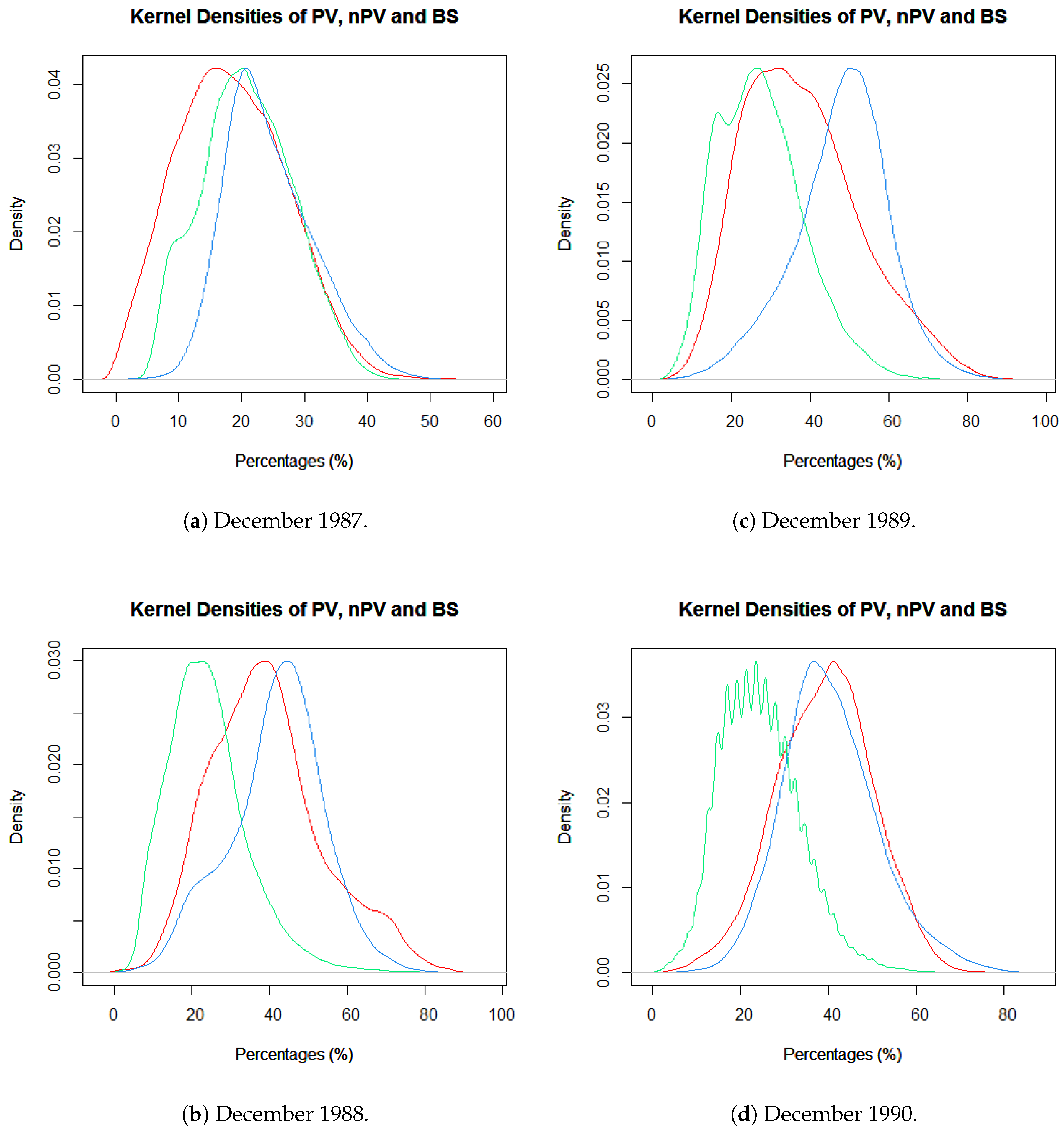
Figure 5.
FCover of Landsat Thematic Mapper (Landsat 5) scenes of four years showing white data gaps caused by masking out clouds and clouds shadows.
Figure 5.
FCover of Landsat Thematic Mapper (Landsat 5) scenes of four years showing white data gaps caused by masking out clouds and clouds shadows.

Figure 6.
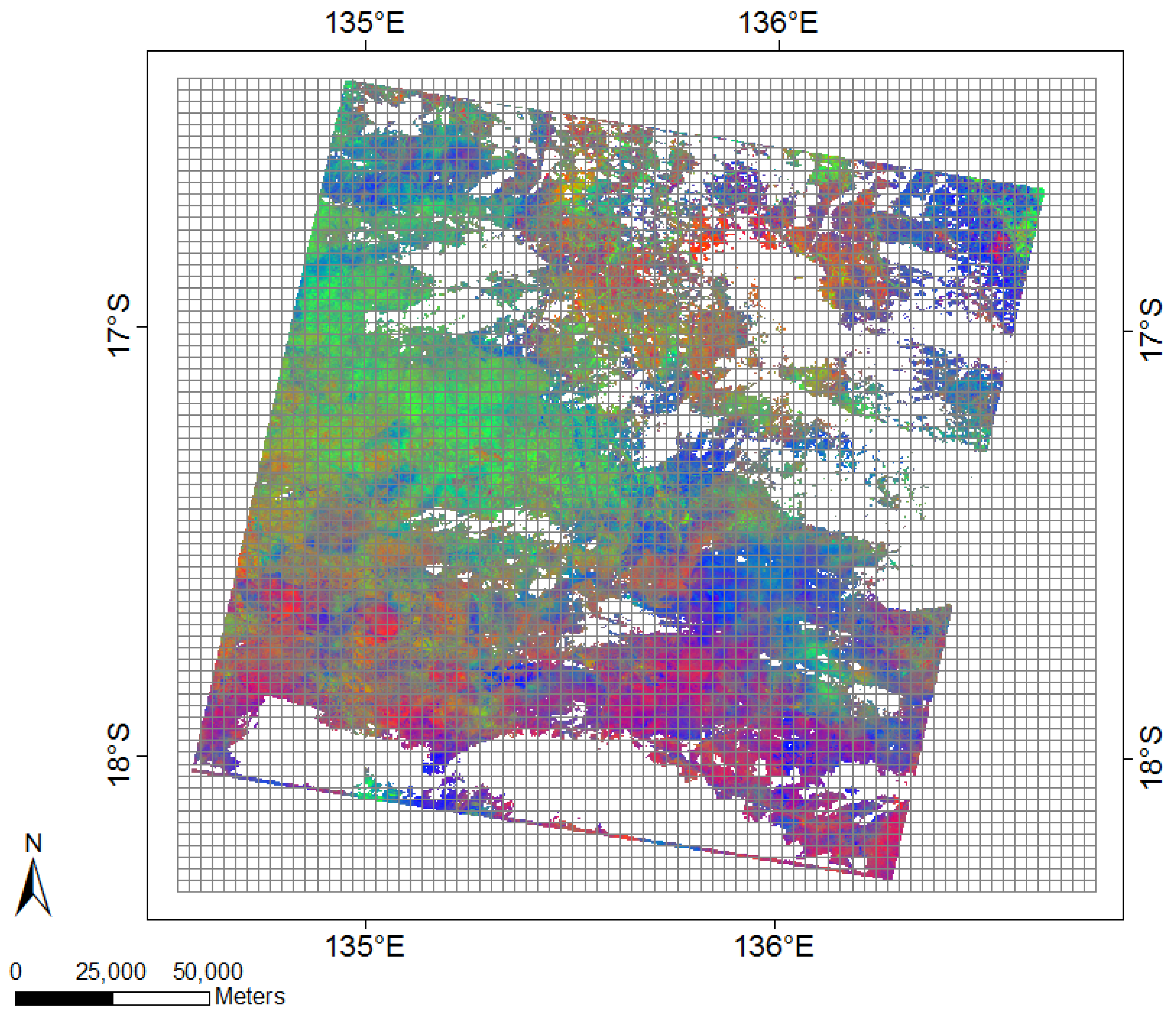
Spatial grid cells at a resolution of 3000 m. The total number of cells 5530. The FCover data are mapped to a even spaced grid where each grid cell contains 100 × 100 pixels and covers an area of 3000 × 3000 m. Please refer to Figure 3 for the triangular ternary diagram for the coloured relationships of the three ground cover types.
Figure 6.
Spatial grid cells at a resolution of 3000 m. The total number of cells 5530. The FCover data are mapped to a even spaced grid where each grid cell contains 100 × 100 pixels and covers an area of 3000 × 3000 m. Please refer to Figure 3 for the triangular ternary diagram for the coloured relationships of the three ground cover types.

Figure 7.
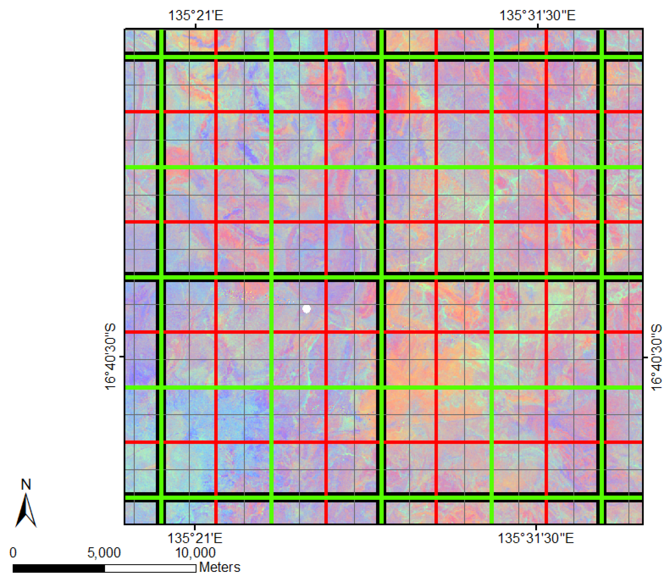
Combination of all four spatial grids used as an overlay for the data delineation of green vegetation fractions out of FCover scenes. The thick black outline shows the resolution in 12,000 m, green in 6000 m, red in 3000 m and thin grey in 1500 m.
Figure 7.
Combination of all four spatial grids used as an overlay for the data delineation of green vegetation fractions out of FCover scenes. The thick black outline shows the resolution in 12,000 m, green in 6000 m, red in 3000 m and thin grey in 1500 m.

Figure 8.
(a) shows the combination of weak learners to one strong prediction rule used in the BRT ensemble approach and (b) illustrated the hierarchical regression and binary splitting process along the branches of the decision tree. (a) Binary splits indicated as red straight lines separate the data in grey and white sections and create weak learners as seen in Equation (1). BRT as an ensemble approach combines them to create complex prediction rules. Adapted from [46]. (b) Hierarchical regression and binary splitting process showing observations in the nodes, predicted values in the terminal nodes and splitting criteria along the tree branches.

Figure 9.
Deviation of residuals around the mean of 1988 in all four resolutions as worst model fit.
Figure 9.
Deviation of residuals around the mean of 1988 in all four resolutions as worst model fit.
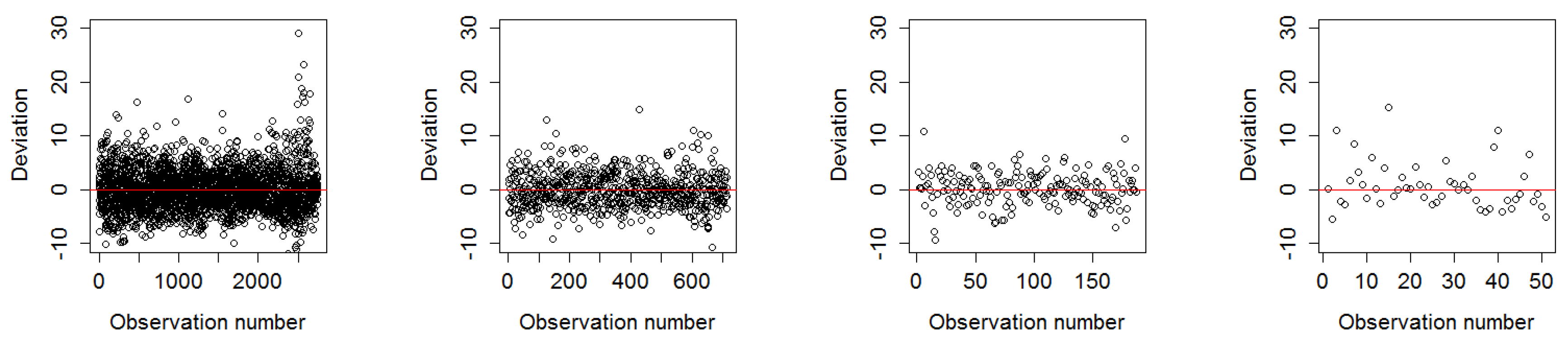
Figure 10.
Deviation of residuals around the mean of 1990 in all four resolutions as best model fit.
Figure 10.
Deviation of residuals around the mean of 1990 in all four resolutions as best model fit.

Figure 11.
Deviation of residuals in all resolutions combined in one plot (left) and corresponding box plots (right).
Figure 11.
Deviation of residuals in all resolutions combined in one plot (left) and corresponding box plots (right).
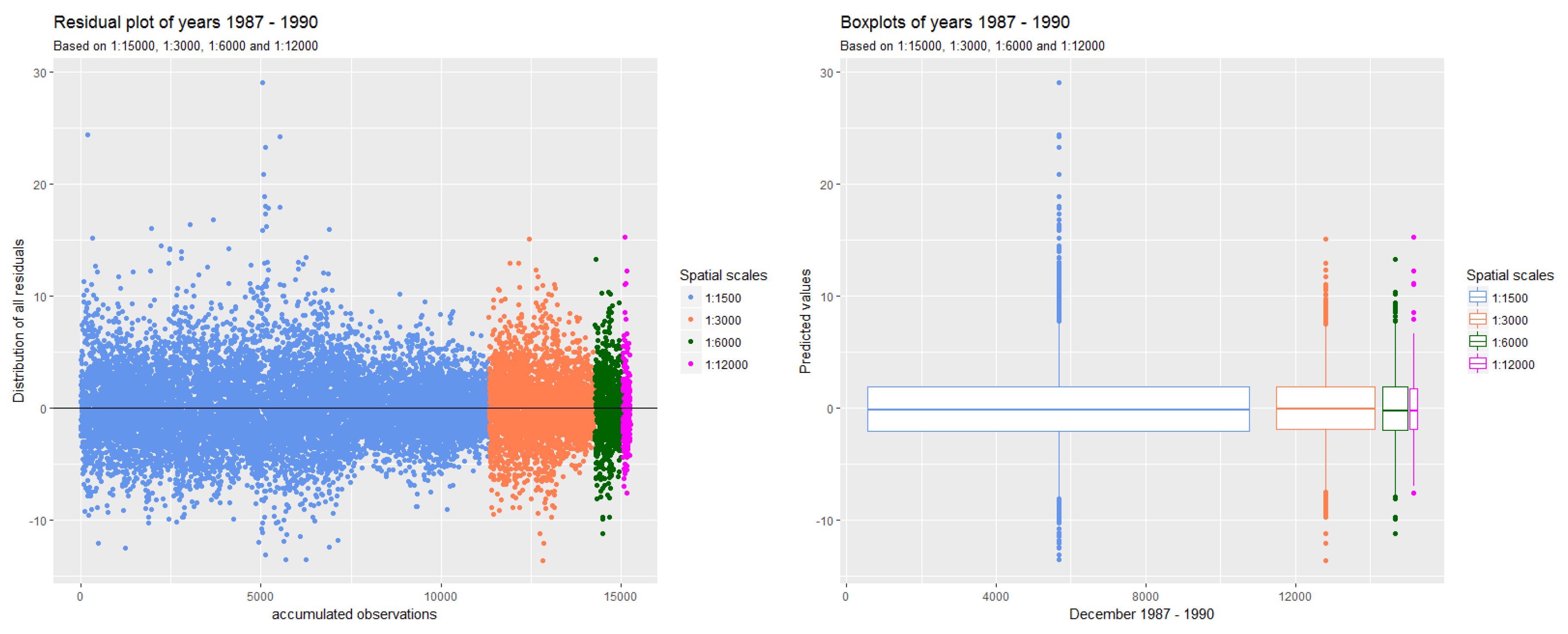
Figure 12.
Relative influence plots of December 1989 in all four resolutions showing the contribution of the centroid coordinate of the latitude (CenterY) and longitude (CenterX).
Figure 12.
Relative influence plots of December 1989 in all four resolutions showing the contribution of the centroid coordinate of the latitude (CenterY) and longitude (CenterX).

Figure 13.
Prediction raster maps for the year 1990. (a) 12,000 m, (b) 6000 m (c) 3000 m and (d) 1500 m.
Figure 13.
Prediction raster maps for the year 1990. (a) 12,000 m, (b) 6000 m (c) 3000 m and (d) 1500 m.
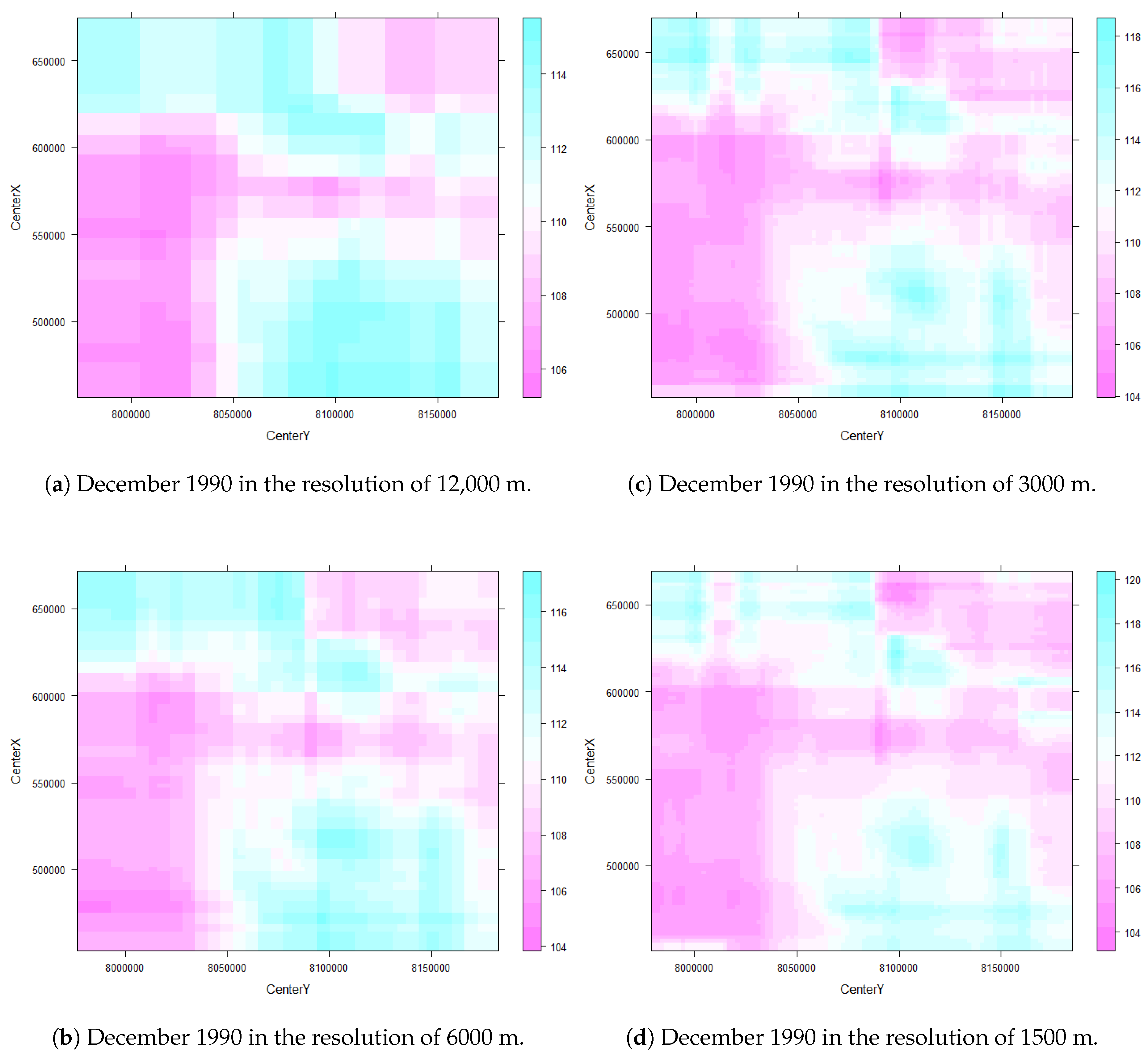
Figure 14.
Prediction surface of 1990 in the resolution of 3000 m.
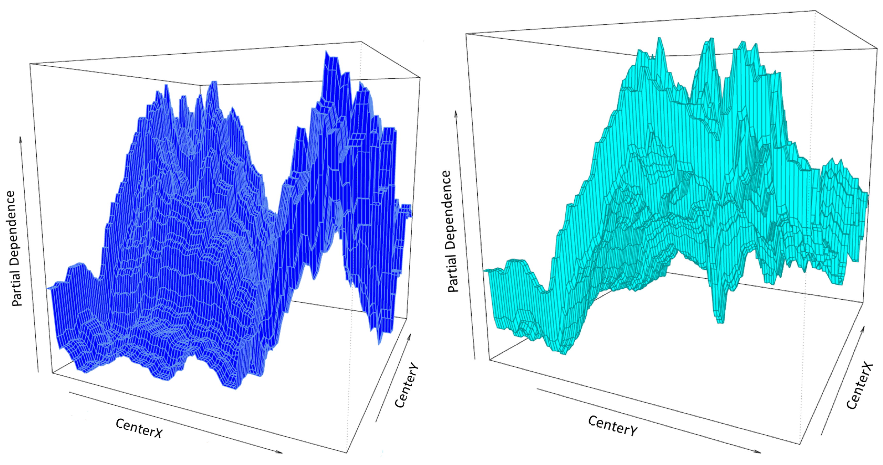
Figure 15.
Marginal plots in the four different spatial aggregation resolutions showing the predicted PV fractions on the y-axis and the observed values on the x-axis.
Figure 15.
Marginal plots in the four different spatial aggregation resolutions showing the predicted PV fractions on the y-axis and the observed values on the x-axis.
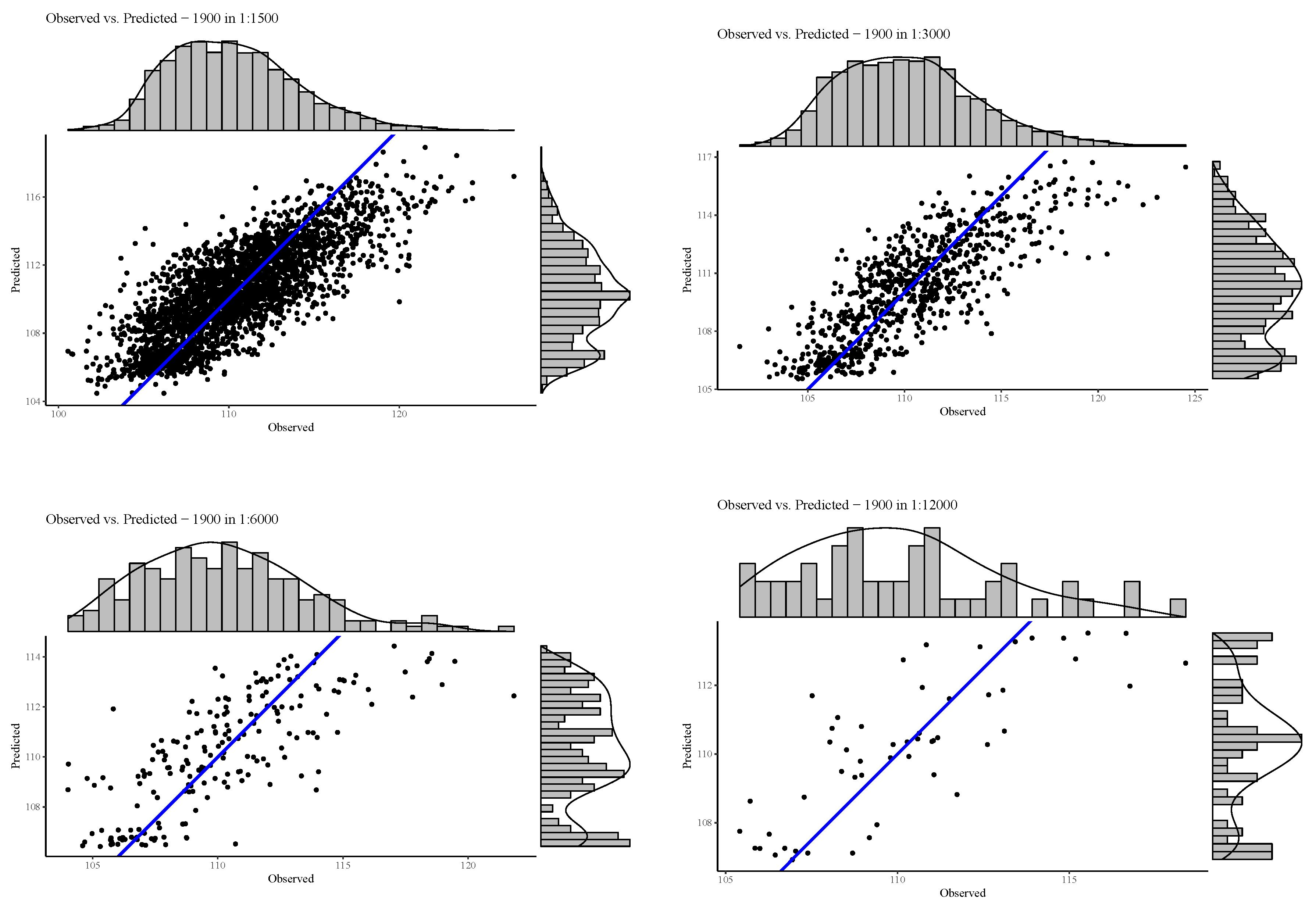
Figure 16.
Comparative information about computational time on (a) the delineation of green vegetation out of FCover imagery and (b) writing to a csv file that will be used as an input file for BRT modelling.
Figure 16.
Comparative information about computational time on (a) the delineation of green vegetation out of FCover imagery and (b) writing to a csv file that will be used as an input file for BRT modelling.

Figure 17.
Quantitative assessment of absolute error rates in the four spatial aggregations.

Table 1.
Table of proposed data reduction scheme. The table shows the smallest resolution of 12,000 m up to the largest resolution of 1500 m and resulting total number of spatial grid cells used for the following spatial aggregation steps. By proposing our data reduction scheme we are not dealing with the original number of 54 million pixels per FCover scene organised in about 7000 rows and 8000 columns.
| Spatial Resolution (m) | Number of Pixels in Grid Each Cell | Ground Covered by Each Grid Cell (m) | Total Number of Grid Cells | Coloured Outline of Spatial Grids |
|---|---|---|---|---|
| original | 1 × 1 | 30 × 30 | 54 million | FCover pixel |
| 12,000 | 400 × 400 | 12,000 × 12,000 | 360 | black |
| 6000 | 200 × 200 | 6000 × 6000 | 1400 | green |
| 3000 | 100 × 100 | 3000 × 3000 | 5530 | red |
| 1500 | 50 × 50 | 1500 × 1500 | 21,980 | grey |
Table 2.
The size of the pre-processed data set varies according to coarseness of the spatial aggregation resolutions.
Table 2.
The size of the pre-processed data set varies according to coarseness of the spatial aggregation resolutions.
| Spatial Resolution (m) | Number of Grid Cells in Overlay | Length of Aggregated Response Variable |
|---|---|---|
| 12,000 | 360 | 360 |
| 6000 | 1400 | 1400 |
| 3000 | 5530 | 5530 |
| 1500 | 21,980 | 21,980 |
Table 3.
Comparison of the RMSE in all four years and resolutions.
| Spatial Resolution (m) | Year | RMSE |
|---|---|---|
| 12,000 | 1987 | 3.0583 |
| 1988 | 3.9691 | |
| 1989 | 3.0056 | |
| 1990 | 1.6151 | |
| 6000 | 1987 | 2.8583 |
| 1988 | 3.1428 | |
| 1989 | 3.1591 | |
| 1990 | 1.9577 | |
| 3000 | 1987 | 3.1120 |
| 1988 | 3.2134 | |
| 1989 | 3.1543 | |
| 1990 | 2.0731 | |
| 1500 | 1987 | 3.4241 |
| 1988 | 3.8306 | |
| 1989 | 3.4500 | |
| 1990 | 2.3348 |
Table 4.
Comparison of RMSE of LM and BRT on worst (1988) and best (1990) model fit.
| Spatial Resolution (m) | 1988 | 1990 | ||
|---|---|---|---|---|
| Linear Model | BRT | Linear Model | BRT | |
| 12,000 | 4.0551 | 3.9691 | 2.7933 | 1.6151 |
| 6000 | 4.9710 | 3.1428 | 3.0449 | 1.9577 |
| 3000 | 5.3688 | 3.2134 | 3.3028 | 2.0731 |
| 1500 | 5.5863 | 3.8306 | 3.5676 | 2.3348 |
Table 5.
MAE and MDAE of the worst (1988) and best model fit (1990) in four resolutions.
| Spatial Resolution (m) | Mean Absolute Error (Worst/Best) | Median Absolute Error (Worst/Best) |
|---|---|---|
| 12,000 | 2.752/1.236 | 2.236/0.836 |
| 6000 | 2.370/1.500 | 1.909/1.185 |
| 3000 | 2.489/1.613 | 2.053/1.305 |
| 1500 | 2.925/1.808 | 2.398/1.467 |
© 2018 by the authors. Licensee MDPI, Basel, Switzerland. This article is an open access article distributed under the terms and conditions of the Creative Commons Attribution (CC BY) license (http://creativecommons.org/licenses/by/4.0/).
Share and Cite
MDPI and ACS Style
Colin, B.; Schmidt, M.; Clifford, S.; Woodley, A.; Mengersen, K. Influence of Spatial Aggregation on Prediction Accuracy of Green Vegetation Using Boosted Regression Trees. Remote Sens. 2018, 10, 1260. https://doi.org/10.3390/rs10081260
AMA Style
Colin B, Schmidt M, Clifford S, Woodley A, Mengersen K. Influence of Spatial Aggregation on Prediction Accuracy of Green Vegetation Using Boosted Regression Trees. Remote Sensing. 2018; 10(8):1260. https://doi.org/10.3390/rs10081260
Chicago/Turabian StyleColin, Brigitte, Michael Schmidt, Samuel Clifford, Alan Woodley, and Kerrie Mengersen. 2018. "Influence of Spatial Aggregation on Prediction Accuracy of Green Vegetation Using Boosted Regression Trees" Remote Sensing 10, no. 8: 1260. https://doi.org/10.3390/rs10081260
Note that from the first issue of 2016, this journal uses article numbers instead of page numbers. See further details here.