Article

On the Very High-Resolution Radar Image Statistics of the Exponentially Correlated Rough Surface: Experimental and Numerical Studies

1
State Key Laboratory of Remote Sensing Science, Institute of Remote Sensing and Digital Earth, Chinese Academy of Sciences, Beijing 100101, China
2
University of Chinese Academy of Sciences, Beijing 100049, China
*
Author to whom correspondence should be addressed.
Remote Sens. 2018, 10(9), 1369; https://doi.org/10.3390/rs10091369
Submission received: 19 July 2018 / Revised: 20 August 2018 / Accepted: 25 August 2018 / Published: 28 August 2018
(This article belongs to the Special Issue Radar Imaging Theory, Techniques, and Applications)

Abstract

:
The aim of this study is to investigate, by means of experimental measurements and full-wave simulations, the dominant factors for the very high-resolution (VHR) radar image speckles from exponentially correlated rough surfaces. A Ka-band radar system was used to collect the return signal from such a surface sample fabricated by 3D printing and that signal was further processed into images at different resolution scales, where the image samples were obtained by horizontally turning around the surface sample. To cross-validate the results and to further discuss the VHR speckle properties, full wave simulations by full 3D Finite Difference Time Domain (FDTD) method were conducted with 1600 realizations for the speckle analysis. At the considered very high resolution, speckle statistics show divergence from the fully developed Rayleigh distribution. The factors that impact on the high-resolution speckle properties from exponentially correlated rough surface, are analyzed in views of the equivalent number of scatterers theory and scattering scales, respectively. From the data results and extended discussions, it is evident that both of the above factors matter for VHR speckle of backscattering, from the exponentially correlated rough surface as a good representative for the ground surface.

Graphical Abstract

1. Introduction

In the context of radar imagery, understanding the speckle properties is imperative for both image de-noising and applications such as land-cover classification and parameters retrieval [1,2,3,4]. Radar speckle arises due to the coherent sum of numerous distributed scattering contributions [3]. A general assumption is the “fully developed” speckle model, which is applicable when the resolution cell size is much larger than the correlation length (l) of the ground surface [3]. This requirement may be met in low-to-medium image resolution. The fully developed speckle model is based on the following two hypotheses: (1) total scattering is contributed by independent scatters; (2) there is a sufficiently large number of scatters contributing to a resolution cell so that a complex Gaussian distribution is followed. For VHR radar images, these assumptions are no longer valid. As a result, the K-distribution is often applied to model the speckles [5,6].
Radar backscattering and its speckle statistic variation with the resolution cell size or antenna footprint has been a subject of interest in rough surface scattering [7,8,9,10,11]. In Reference [7], the convergence of backscattering coefficients versus footprint size was studied by 1-D method of moment solution. By theoretical models and indoor SAR experiments in EMSL. In Reference [8,9], the dependence of polarimetric backscattering characteristics from Gaussian correlated rough surfaces on the SAR resolution cell size was examined, while the SAR images of rough soil surfaces were measured in EMSL [10]. That work includes results and analysis on the backscattering coefficients and image probability density functions (PDF), versus different resolution cell size. As the radar image resolution reaches from tens of meters to approximately 1 meter, or even a smaller size, this topic becomes more important currently for land observations. In order to model high resolution speckle properties, Di Martino et al., proposed the predicting method for the equivalent number of scatterers within the resolution cell [11], considering stochastic stationary rough surface description and more advanced, fractal surface models. In this work, we address the topic of VHR radar speckle statistics using indoor SAR experiments and supporting full-wave simulations.
Since the prediction for the equivalent number of scatterers has been established in Reference [11], it is used as an evaluating tool in this work. To be specific, the exponentially correlated rough surface is considered, due to its rich high frequency roughness on the surface-air interface that leads to numerous local scattering contributions. In particular, 3D printing process was used to fabricate the sample surface that is used for scattering measurement conducted at Ka band. In this manner, the image resolution scale close to the rough surface correlation length can be achieved, namely, the image resolution cell size can be at the same scale of the surface geometric undulation. In this view, the scattering mechanism from exponentially correlated rough surface is similar to that from sea surface, where scattering process from short scale roughness is modulated by relatively long scale undulation [12,13]. The prediction for the equivalent number of scatterers per resolution cell from [11] is served as a reference in the analysis. Meanwhile, based on the results from experimental and supporting numerical practices considering different incident directions, the effects of scattering scale on the speckle properties can be observed. Further numerical studies are conducted with different RMS height, for discussions on both the factors of the equivalent number of scatterers and the scattering scale effects.
Similar to the work in Reference [10], we focus, in this study on the VHR radar speckles from the exponentially correlated rough surface. Also, the numerical studies by 3D-FDTD simulations are used to support the data analysis to exploit the physical process. The remainder of this paper consists of 4 parts. In Section 2, the rough surface sample generation, the experimental and numerical methods, are demonstrated with verification results. In Section 3, the measured images, simulated backscattering and their amplitude statistics are presented. In Section 4, the equivalent number of scatterers and scattering scaling effects are considered to analyze the speckle results. Then with extended numerical results, the VHR radar speckle properties are further discussed with consideration of both the factors. Finally, the contribution of this work is highlighted in the conclusion.

2. Experimental and Numerical Methods

In this work, to study the VHR rough surface speckles, both the experiments and full-wave numerical simulations are conducted. In this section, the configurations and procedures are to be demonstrated.

2.1. The Rough Surface Samples

In this paper, an exponential correlation function for the random rough surface is used since it describes better for the natural ground surface [4]. For both the experimental target fabrication and numerical discretization, digital samples are generated. Specifically, the spectrum method is used to generate digital samples, as that: by generating the roughness spectrum components with random phase and amplitude distribution following Equation (1), then performing inverse Fourier transform, one obtains the digital sample. The statistical roughness parameters of the rough surface samples are listed in Table 1. In addition, the roughness spectrum of the exponential correlation surfaces is plotted in Figure 1.
W ( k ρ ) = h 2 l 2   2 π ( 1 + k ρ 2 l 2 ) 3 2
where h is surface RMS height and l is correlation length (autocorrelation length).
In fact, it has been difficult to actually fabricate an exponentially correlated experimental sample, due to the rich high frequency roughness. In this work, the 3D printing technique was utilized for the fabrication. This technique allows one to directly manufacture actual samples based on the computer-generated digital sample with designed parameters, as shown in Table 1. In Figure 2, the CAD model and actually fabricated sample for the experimental study are presented. As should be noted, the considered sample has rich high frequency roughness, which generates numerous local scatters, leading to the strong speckle effects.
More specifically, the FDM (Fused Deposition Modeling) technique is utilized for the fabrication. In this 3D printing process, very thin lines of fused materials are continuously printed to construct a structure and a 100% filling rate can be achieved to form a solid. By this way the shaping accuracy of about 0.5 mm can be achieved, which is approximately λ/20 in the Ka band and sufficient for the imaging study. The main advantage of this technique is that it permits the usage of lossy material, so as to generate samples simulating the half space rough surface scattering scenario, such as the moist soil ground. In this work, the measured permittivity is 6.22-j2.86 at 32 GHz and that value was used in the FDTD computations.
On the other hand, in order to obtain the speckle results numerically, one requires a large number of digital surface samples to accomplish a statistical simulation [4]. In this work, the following procedures are excised: first a very large rough surface mesh is generated on grids, then the digital sample for each realization (400 × 400 meshing points) is cut from that large mesh. In the cutting, one sample is neighboring and overlapping to next with 100 discretize interval (100 × interval size ~31 mm) distant, which is close to the footprint size in diameter in the numerical simulations. For the speckle study, 1600 (40 × 40) samples are obtained for one to achieve an enough number of realizations. The digital samples are then input into the FDTD simulator one by one for computing scattering in the 3D computational domain.

2.2. Experimental Configuration and Procedure

The experimental imaging system is constructed based on a vector network analyzer (VNA) and a 1D scanner, as shown in Figure 3. To achieve the rough surface imaging in the chamber, the measurements are performed in the Ka band. Detailed configuration parameters include: the track span (L) is 800 mm with an interval of 8 mm; the distance between the target scene center and the antenna (T/R) is approximately 1400 mm; the transmitting and receiving antennas are of 20 dBi gain with a half power beam angle of 17°. In the implementation, the height difference H and distance D can be varied accordingly to achieve the beam direction or incident direction angle θi of 30°, 40°, 50° and even 60°. The target is placed on a low-scattering supporting cylinder made of the foam material, which is set on a motor driven rotation platform (for φ rotation as shown in Figure 3). Multiple image acquisitions should be achieved for the speckle statistics. More specifically, in each case of θi, the imaging measurements for the rough surface sample are performed 20 times and after each time φ is changed with an equal angular interval, as shown in Figure 3. Therefore, 20 images are obtained for a specific θi, then speckle statistical analysis can be conducted based on those results.
In the scanning measurement, the scattering signals were captured through the antennas and VNA all along the scanning track and all over the Ka band. Then different bandwidths and synthetic aperture lengths were selected to achieve different spatial resolutions (in ground range), as concluded in Table 2. During the image processing, the Kaiser window (β = 2.5) was utilized along the frequency and aperture signal. And the resolution cell size in Table 2 are realized in the presence of the Kaiser window.
For radiometric calibrate, one metal sphere of 30 mm in diameter was used as the RCS reference. However, to study the speckle statistics of image amplitudes, ideally the rough surface sample should be uniformly illuminated by the transmitting antenna and uniformly viewed by the receiving antenna. Unfortunately, the antenna patterns are not uniform on the measured sample and their effects must be compensated, including those of both the transmitting and receiving antennas. In addition to the RCS calibration with one metal sphere and the range amplitude compensations commonly implemented in SAR processing, we further measured the images from a column of 3 metal balls in the ground range direction. Based on the image of these balls, the antenna pattern weighting was fitted along the range and that fitted weighting function was then utilized to compensate the image amplitude, as shown in Figure 3 and Figure 4.
Finally, after the images from the rough surface were processed, calibrated and compensated, the amplitude speckle results were obtained for the VHR radar speckle analysis.

2.3. Numerical Simulation Configuration and Procedure

Although the experimental study is the most straightforward and reliable approach, it is restricted by the actual rough surface sample in both the aspects of number and size. On the other hand, the full-wave full-3D Finite Difference Time Domain (FDTD) simulator provides with complementary and extensible data support. This numerical method has been reported in computing scattering from layered and heterogeneous rough surfaces [14,15]. The FDTD simulator used in this work is developed based on that reported in reference [16] which is a full-3D simulator and by performing simulations on a large number of samples (realizations) one can get the backscattering results for speckle analysis as well as averaged scattering coefficients.
Figure 5 shows the simulation configuration in each realization, which is a typical scene for the half-space scattering. In general, the tapered incident beam is injected by the Total Field/Scatter Field boundary (TF/SF), below that boundary the incident beam immerges to illuminate the rough surface and above that the boundary scattered field can be extracted. The Huygens Aperture collects the recorded near-field scattered field and turns that into far-field results like scattering coefficients. On the other hand, the Perfect Matching Layer (PML) is used to truncate the computation domain without introducing disturbing reflections.
In this work, a tapered wave with the fixed ground footprint is set for the illumination. In each realization, the incident beam is always pointing to the center of the rough surface. In this work, different incident angles θi are considered, namely, 30°, 40° and 50°. Furthermore, cases of different surface RMS heights h are also considered to support the extended discussions. The discretization cell size in the FDTD simulation is set to 1/30λ at 32 GHz, which is sufficient in modeling the high frequency roughness of the exponentially correlated rough surface.
In general, the aim of this simulation work, which is similar to that reported in Reference [4], is to investigate speckles by counting backscattering far-field amplitude results over a large number of realizations. The difference is that we focused on the VHR situation, which means we used a smaller tapered wave illumination region than those in the general rough surface scattering simulations. Specifically, the simulated resolution cell size is defined by the beam footprint in the numerical studies, realized by setting the footprint size equal to the required value (30 mm in a diameter for 3 dB edge power drop). The detailed computation parameters are summarized in Table 3 and these simulations are performed to support the conclusions drawn from the VHR radar imaging experiments with a 30 mm resolution as well as further discussions. The simulations were run on a 2-way Intel Xeon workstation with octal channel memories: one set of 1600 realizations required approximately 1 week, with each realization taking less than 5 min.

2.4. Verification Results with AIEM

In this section, we present the verification results to validate the fabricated experimental sample and the utilized numerical simulator, with the reference of results by the Advanced Integral Equation Method (AIEM) [17] for the rough surface scattering. The AIEM model results from an approximate but accurately enough solution of integral equations that govern the surface fields. It has been proven that the AIEM model is able to accurately predict the scattering from randomly rough surfaces. The detailed formulation of the AIEM model can be found in Reference [17,18] and a recent application example in scattering from rough soil surfaces is referred to [19].
First, to validate the fabricated sample for the experimental imaging tests, we directly measured its scattering coefficients without imaging process. Since in the scattering coefficient measurement only one data sample can be obtained through one measurement, apparently more angular samples (in φ) are needed than those for the imaging measurement. Actually, more than 48 sets of backscattering data were obtained by the φ angle rotation in this case. The backscattering RCS data were obtained with the calibration by the metal sphere and then normalized into scattering coefficient, by the actual section of the rough surface sample. The measured scattering coefficients are compared with the AIEM model predictions at different θi, clearly, good agreement can be observed in the Figure 6.
Secondly, to validate the FDTD simulator, the computational domain was increased to 1200 × 1200 × 180 Yee cells in the domain size, so as to obtain converged scattering coefficients. In other words, the rough surface aperture size was increased to 40λ × 40λ. It should be noted that, in common scattering simulations for rough surfaces [4], the aperture size of 32λ × 32λ is electrically large enough. Because of the huge computational burden, with one realization requiring approximately 1 h, only 50 realizations are performed to obtain the averaged scattering coefficients distributions over the upper space. Again, the AIEM results are utilized as reference and two sets of results are compared in Figure 7. Although the FDTD results failed in presenting a smooth contour due to the insufficiently large realization number, the results by numerical and analytical methods clearly agree well with each other in the distribution patterns.

2.5. The Differences in Experimental and Numerical Studies

Before the results are presented and discussed, there are some differences in the experimental and numerical configurations that should be concluded and noted, for referencing purposes.
First, in the experimental study, the image results are obtained in RCS with unit of m2; while in the numerical study, the scattering coefficients without unit of m2, are computed without imaging process. To make a direct correspondence for the speckle results, the PDF of the measured image amplitudes and the simulated scattering amplitudes are normalized by the averaged intensity (RCS σRCS in experimental images and scattering coefficient σ0 in numerical simulations), respectively. The averaged σRCS from the experimental images can also be normalized into σ0 by using:
σ 0 = σ R C S   S i , S i = ρ g r ρ a cos ( θ i )
where ρgr and ρa are the ground range resolution and azimuth resolution, respectively.
In the experimental measurement, sufficient measurement samples are gathered by rotating the sample surface in azimuthal direction. In the numerical simulations, a large number of realizations are simulated for the speckle analysis.

2.6. Speckle Description

Based on the measured images and the simulated backscattering returns, the speckle properties can be obtained.
First, the PDF can be computed for the amplitude and compared to the well-known Rayleigh distribution and K-distribution. The equations of the two aforementioned PDF models can be found below. The Rayleigh distribution for the fully developed speckle takes the form:
p R ( A ˜ ) = 2 A ˜ e A ˜ 2   , A ˜ 0 A ˜ = A < A 2 >
where A ˜ is the amplitude normalized by the square root of mean intensity (I = A2). The K-distribution, is given by
p K ( A ˜ ) = 4 α ( α + 1 ) / 2   Γ ( α ) A ˜ α K α 1 ( 2 α A ˜ ) , A ˜ 0
where α is the shape factor coefficients. A larger α will push the K-distribution closer to the Rayleigh distribution that describes the fully-developed speckle. The α value for the K-distribution fitting are obtained by the fourth order moment of < A ˜ 4 > (i.e., second order moment of mean normalized intensity), using:
< A ˜ 4 > = ( 1 + 1 α ) ( 1 + 1 N l o o k   ) α = 1 / [ ( < A ˜ 4 > / ( 1 + 1 N l o o k ) ) 1 ]
The standard deviation to mean ratio (γ) of the amplitude can be obtained as:
γ = [ var ( A ) ]   1 / 2 A
where γ can also be used to check the speckle properties. For reference, the fully developed speckle whose amplitude PDF follows a Rayleigh distribution, is with a theoretical value:
γ R = 4 π 1   0.5227

3. Analysis on the Experimental Imaging and Numerical Results

In this section, the imaging results from the rough surface sample, the image amplitude speckle statistics and the numerical results are to be presented.

3.1. Imaging at Different Resolutions and Incident Angles

In Figure 8, the image examples of the exponentially correlated surface are presented at different resolution scales and different values of θi. The scattering hot-spots at a VHR scale are observed to be fused into those at the lower resolution scales. In addition, clearly, as θi increases, the RCS of those spots decrease. The presented images are obtained at one of the 20 φ positions and along with the results at other φ positions, they are used to produce the speckle results.
In Figure 9 and Figure 10, the image amplitude PDFs are plotted and compared to the Rayleigh distribution and the fitted K-distribution. In each sub-figure of Figure 9, the fitted α for the K-distribution is marked, where the resolution cell size is set to 30 mm (in azimuth and ground range), or in correlation length, 0.63l. Clearly, at the smallest θi of 30°, the fitted α is the smallest and the PDF curve is with the tail in semi-log plot most away from the Rayleigh curve. This fact is also observed in Figure 10, the results in which are with a resolution cell size of 60 mm, or in correlation length, 1.25l. Meanwhile, as the resolution cell size enlarges from 30 mm to 60 mm, the fitted α of K-distribution at each θi gets larger and the corresponding PDF is closer to the Rayleigh reference. That agrees with the common sense. On the other hand, it should be noted that the PDFs in case of resolution cell size 60 mm (Figure 10) is not fitting the K-dis as well as those in the case of resolution cell size 30 mm (Figure 9). That is due to the limited size of the sample (250 mm in diameter), as it becomes insufficient in providing with rich enough scatter returns with increasing resolution cell size.
After the amplitude PDF results based on experimental images are presented, the corresponding averaged RCS σRCS, the averaged scattering coefficients σ0, the fitted α of the K-distribution and the computed γ are listed in the Table 4 for referencing purpose. Further, the computed γ in case of different θi are plotted via resolution cell sizes in Figure 11. The coarse but not perfect trends can be well observed, that the γ curves are approaching to the γR = 0.5227 with the rising of the resolution cell size. The imperfection in those trends is also due to the limited sample size. Also in Figure 11, the results of computed γ results without antenna pattern compensation conducted in the imaging process are also presented, showing the necessity of such a treatment in the chamber imaging experiments for speckle properties.

3.2. Results of Numerical Simulations

Next, the numerical results of 1600 realizations are to be presented, the parameters for this set of simulations are concluded in Table 3(set 1). For reference purpose, first, the simulated scattering coefficients over the upper space (bi-static) are presented in Figure 12, including results by one realization and averaged results by 1600 realizations, in cases of θi = 30°, 40° and 50°. It can be clearly observed that, after averaged over 1600 realizations, the computed bi-static scattering coefficients converges to a smooth distribution.
Then the backscattering amplitude PDF results in cases of θi = 30°, 40° and 50°, are compared in Figure 13, with a 3 dB footprint size of 30 mm in diameter. It is very clear that, from θi = 30° to θi = 50°, the larger θi leads to larger fitted а and the amplitude PDF is closer to the Rayleigh distribution. That trend has also been observed in PDF results from measured images (Figure 9 and Figure 10). For reference, the averaged backscattering σ0, fitted α for K-distribution and computed γ are concluded in Table 5. As can be observed from the results in Table 5 and Table 6, both the experimental imaging and numerical simulation statistics show the same trend, that a larger θi (from 30° to 50°) leads to the γ closer to the fully developed γR. That is, as the θi get larger in the moderate region, the observed VHR speckle of the exponentially correlated sample approaches toward the fully developed speckle.

4. Discussion

In this section, the simulation results are discussed in the view of the equivalent scatter numbers and scaling effect. Then further numerical studies are presented to discuss the effects of the two factors on the VHR speckle properties from exponential correlated rough surface.

4.1. Equivalent Scatterer Numbers Prediction

It is well known that the high-resolution speckle properties are different from the fully developed speckle that in the case of low resolution. Driven by the trends of high resolution imaging system development and deployment, it becomes increasingly desired to model the high-resolution speckle for land observations. Starting from the low-resolution basis, the amplitude PDF of Rayleigh is built on the condition that many independent scatters contribute to one resolution cell. It is straightforward to explore new speckle descriptions based on the concept of equivalent number of scatterers [5,11].
The K-distribution, especially for the speckle intensity PDF, has been derived based on the mathematical concept of coherent sum of a finite number of field returns [5]. In that derivation, each of the independent scatters is assumed to be K-distributed in amplitude and uniformly random in phase. Under these assumptions, a close form of K-distribution intensity PDF was obtained. For considering image speckle, the number of scatters per resolution N is an important factor and it is proportional to α of the overall K-distribution.
In Reference [11], the prediction model for the equivalent number of scatterers per resolution cell was proposed based on the concept of sub-area dividing, to quantitatively predict the speckle properties of rough surfaces in high resolution observations. The objective of Reference [11] was to provide a quantitative description linking the equivalent number of scatterers N to the well-established K-distribution, that a larger N generally leads to speckle closer to Rayleigh and a smaller N may lead to a K-distribution further away from the Rayleigh model. A compact formulation is given as in Equation (8), yielding the equivalent number (N) of distributed scatters within a resolution cell size with respect to surface correlation function types, parameters, incident direction and observation frequency [11].
N = A e / π 2   [ ln ( 1 t 4 k z 2 σ 2 ) ] 2 / n = N ( A e π 2 , k z σ , n )
where kz = k*cos(θi), Ae is the area of a resolution cell (not image pixel and n is 1 for the exponential correlation, 2 for the Gaussian correlation function, with t = 1 [11].
It should be noted that the α of the overall K-distribution is also proportional to α of the sub-scatters (αs) and a relationship can be concluded as α = N*(αs). It is also important that in the rough surface scattering, the αs namely the K-distribution parameters for the “independent scatters” may vary according to surface roughness parameters and incident angle θi. It is possible that in the radar image speckle from rough surfaces, if there is only one equivalent scatter in a resolution cell but the scatter is with Gaussian statistics (αs is very large), then the overall image speckle properties acts as fully developed. On the other hand, if there is a sufficiently large N so that N*(αs) is sufficiently large, then the overall image speckle properties also act nearly as fully developed.
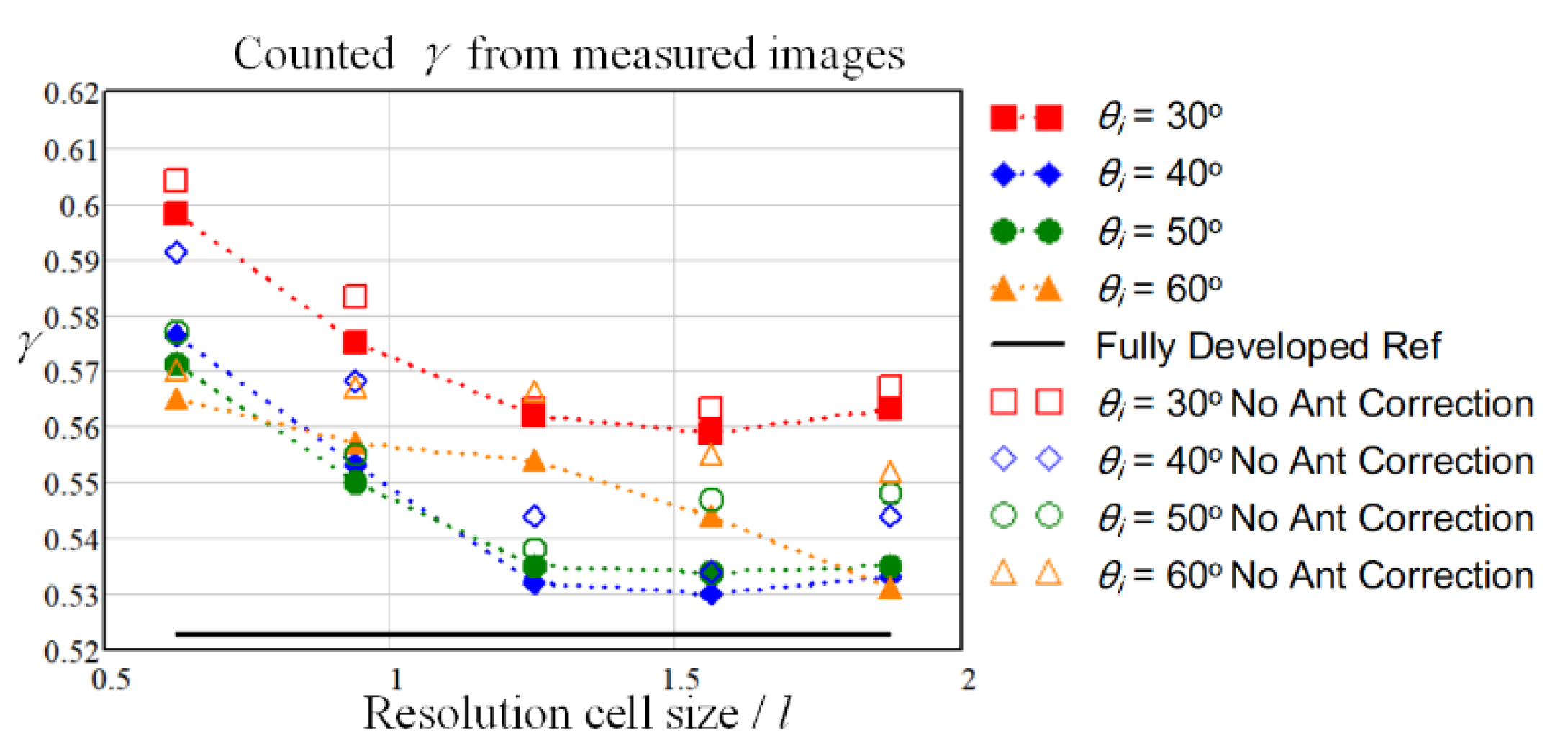
The experimental results that larger resolution cell size leads to a more Rayleigh distribution, agrees with common sense, as well as the theory prediction for equivalent number of scatterers. In that theory, as the resolution cell size gets larger, the equivalent scatterer number N gets larger while αs keep unchanged, therefore the speckle properties approaches to the Rayleigh model.

4.2. Similarity to Sea Surface Scattering-Scattering Scaling Effects

In this work, the focus is on the scattering from exponentially correlated rough surface, especially when the resolution is at the level of correlation length. This is a case that will be encountered in the SAR observations of land surface, as the resolution performance keeps evolving. On the other hand, since the correlation length (l) of the sea surface is much larger so that the SAR imaging resolution is already at the level of l, the non-Rayleigh speckle phenomenon in sea speckle has been widely noticed and studied for decades [5,12,13,20,21,22].
Specifically, the K-distribution has also been derivated for modeling sea speckle as a compound PDF in Reference [12]. In that derivation, the radar speckle is viewed as a multiplicative process z = xy, where the random process y has Rayleigh PDF, with its power modulated by the process x which is assumed to follow the Gamma distribution. The above mathematical description goes along with the physical understanding of two-scale model for the rough sea surface scattering at intermediate incidence angles [13]. In this case the backscatter can be regards as a collection of the small/middle scale returns from the local surfaces such as the Bragg scattering (process x), while the strength of those returns is modulated by the long scale undulation of the surface through tilting and other mechanisms (process y). Apparently, both the scattering from short scale roughness and long scale roughness modulation are functional for the total scattering.
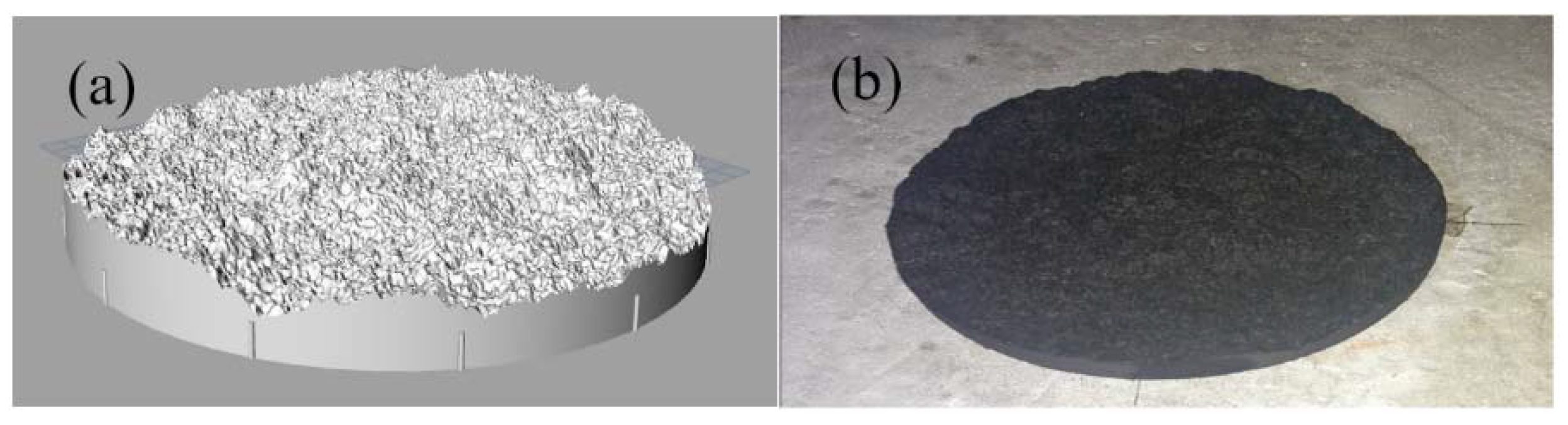
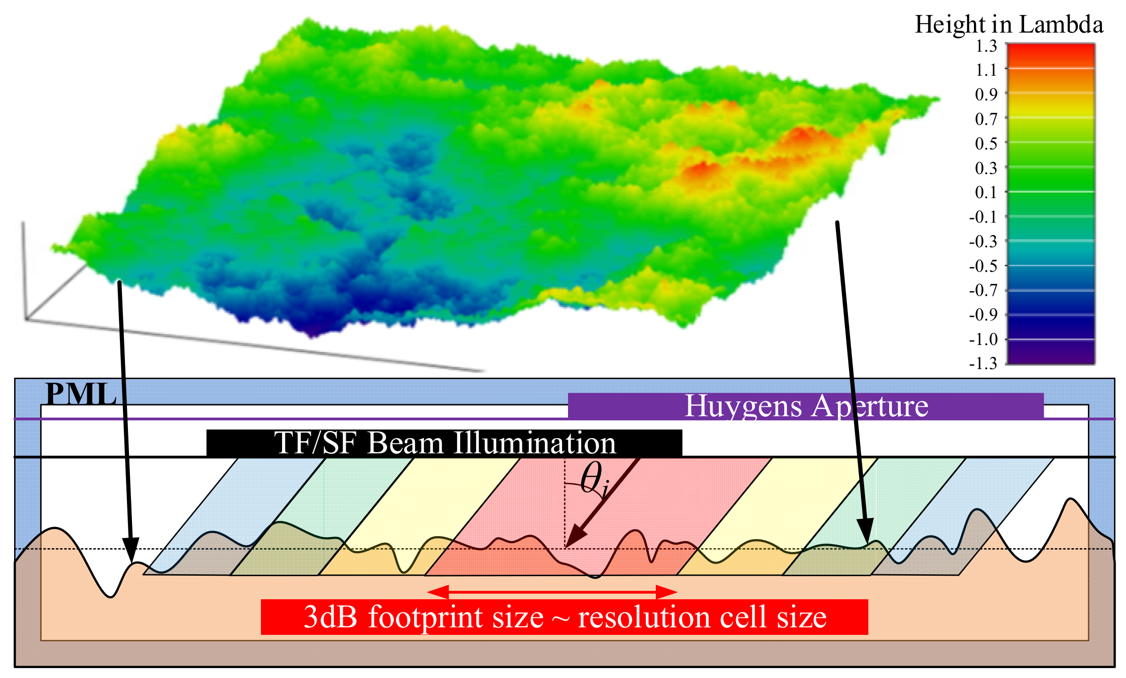
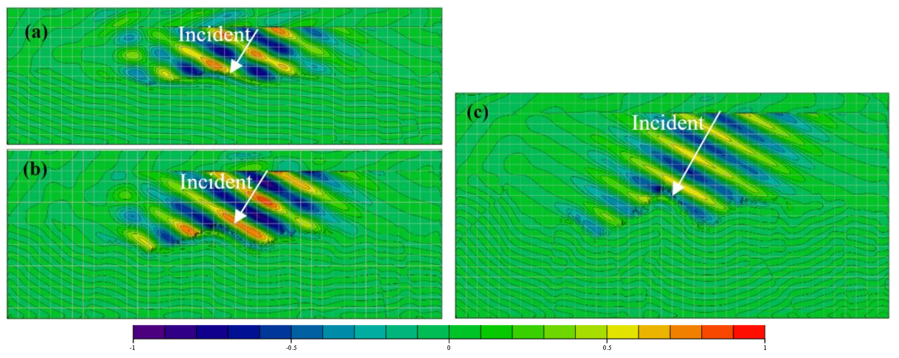
Actually, one can find the similarity of the scattering process from exponentially correlated rough surface to that from sea surface, especially when the resolution cell size is close to the correlation length. In this case, the exponentially correlated rough surface contains rich high-frequency roughness leading to scattering source all over the surface as the scattering from short-scale roughness (as can be observed in Figure 14 along the surface interface), meanwhile the undulations at the level of correlation length (long scale roughness) provide with the relatively long scale modulation carrier. The difference in the mechanisms between the scattering from the exponentially correlated rough surface observed in high resolution, to that from sea surface, is due to the lack of intermediate scale Bragg scattering. Because for an exponentially correlated surface there is no wind driven periodic undulation structure.
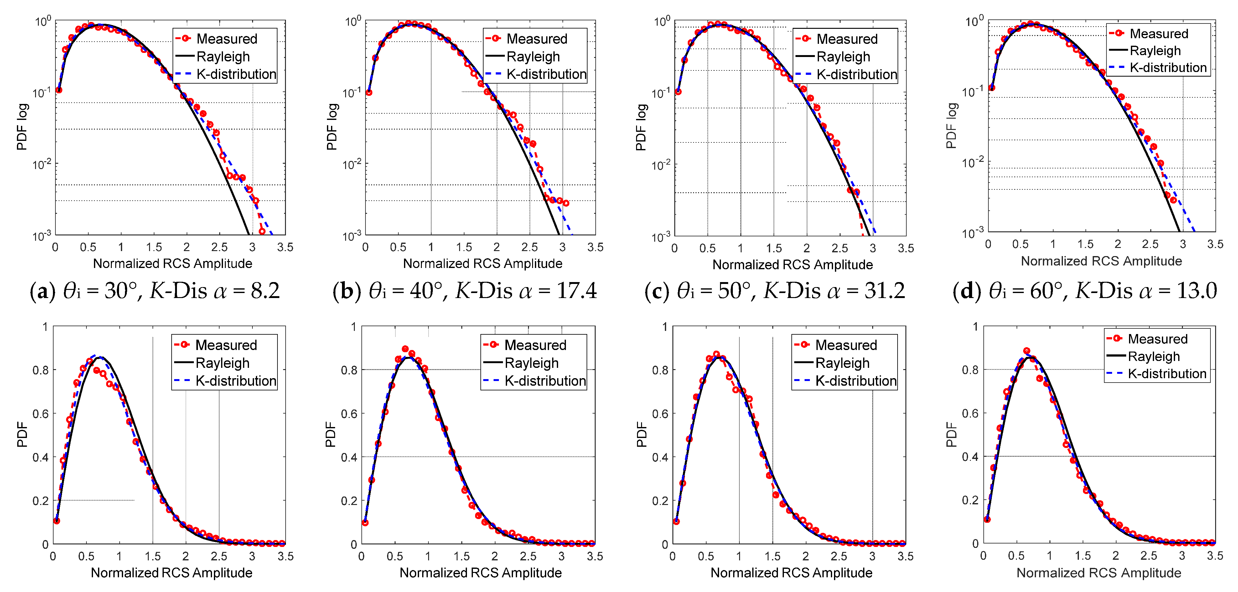
From both the experimental and numerical results at the very high resolution, it is interesting that when the incident angle θi gets larger from 30° to 50° (moderate region), the speckle are approaching towards the fully developed Rayleigh description. The answer to this phenomenon, however, can also be found from the knowledge in scattering mechanisms from sea surface [22,23,24]. In Reference [24], the scattering mechanisms were discussed in the aspects of roughness scales for the two-scale or more precisely multi-scale sea rough surface. Specifically, the wavelength filtering effect is states that when the incident angle becomes larger, the dominating factor shifts from long-scale roughness towards short-scale roughness [22,23,24]. And for the vertical polarization, this effect is more notable than that of horizontal polarization [24]. If the effect of long-scale roughness is weakened enough due to the enlarging of θi in the moderate region, then the multiplicative process is weakened because that the scattering from short-scale is taking the dominance of scattering mechanism, as well as the speckle properties. And the scattering from short scale roughness most possibly follows a Rayleigh PDF. It is interesting that, from the results of simulated sea backscattering in Reference [21], one can find that the speckle PDF results is also approaching toward Rayleigh when θi get larger in the moderate region.
Based on the rich knowledge from the research on sea surface scattering, the observed VHR speckle variation from exponentially correlated rough surface in the moderate θi region, can be clearly explained: the multiplicative effect of scattering process is weaker when the θi get larger from small to moderate, as the effects of carrier long-scale roughness gets weaker. In this case, because the scattering from short scale roughness gets more dominating as the θi get larger and itself acts as Gaussian, the overall speckle distribution approaches towards the Rayleigh model.

4.3. Further Discussions on the Two Factors

The widely applied K-distribution in modeling non-Rayleigh speckle, can be either descripted based on the concepts of equivalent number of (independent) scatter N [5,11] and the two-scale scattering of multiplicative process [12,
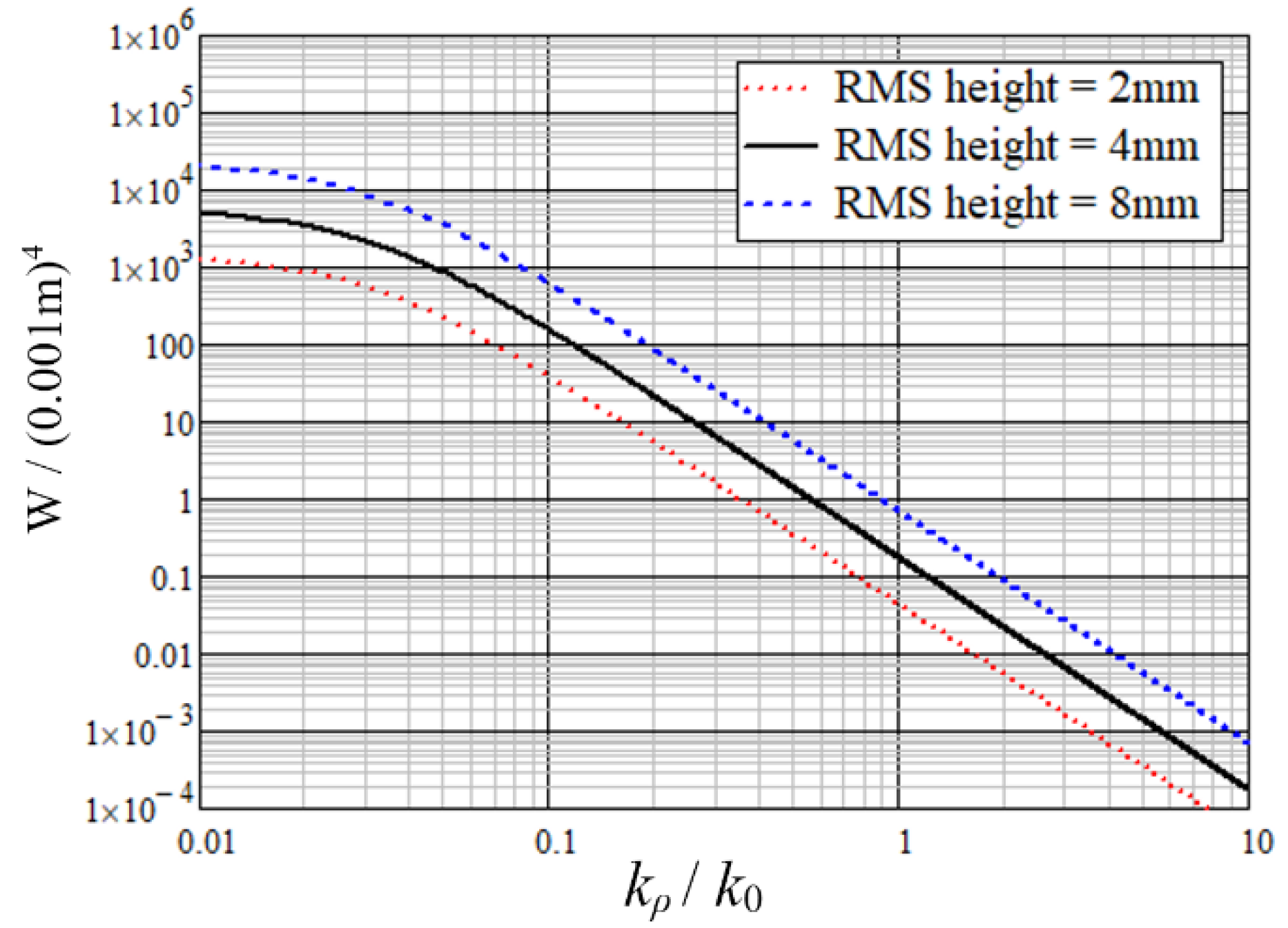
13]. To further explore the VHR speckle properties from exponentially correlated rough surface as a significant description for ground roughness and to discuss the dominating factors, another set of computations are performed for analysis (parameters in Table 3(set 2)). Specifically, different RMS height h are considered: 2 mm (0.21λ), 4 mm (0.43λ), 8 mm (0.85λ), 12 mm (1.28λ@32 GHz) at θi = 30°. For each cases of h, still 1600 realizations are computed for the speckle analysis. In Figure 14, the recorded Electric fields at 32 GHz in the incident plane cut of the computation domain in one specific realization were presented, as an intuitive exhibition for the difference of scattering process in case of different h. It seems that, when h = 4 mm, occasional specular reflection may contribute to the backscattering of θi = 30°. Actually as shown in the scattering coefficient results of Figure 15, the backscattering at h = 4 mm is larger than those at h = 2 mm, h = 8 mm and h = 12 mm. In 
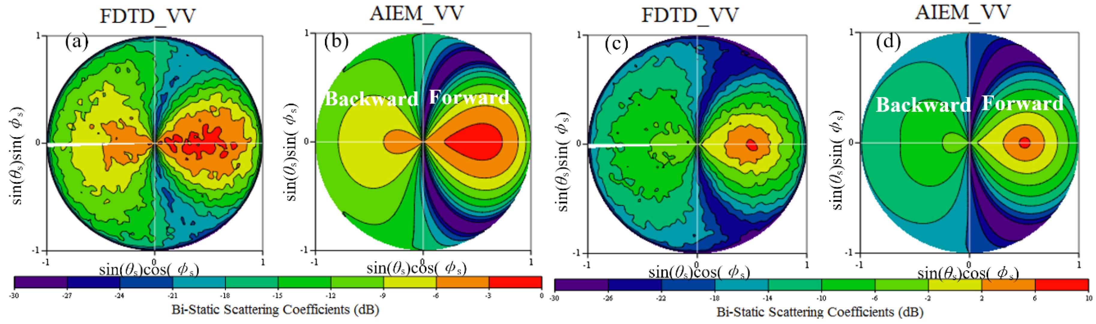
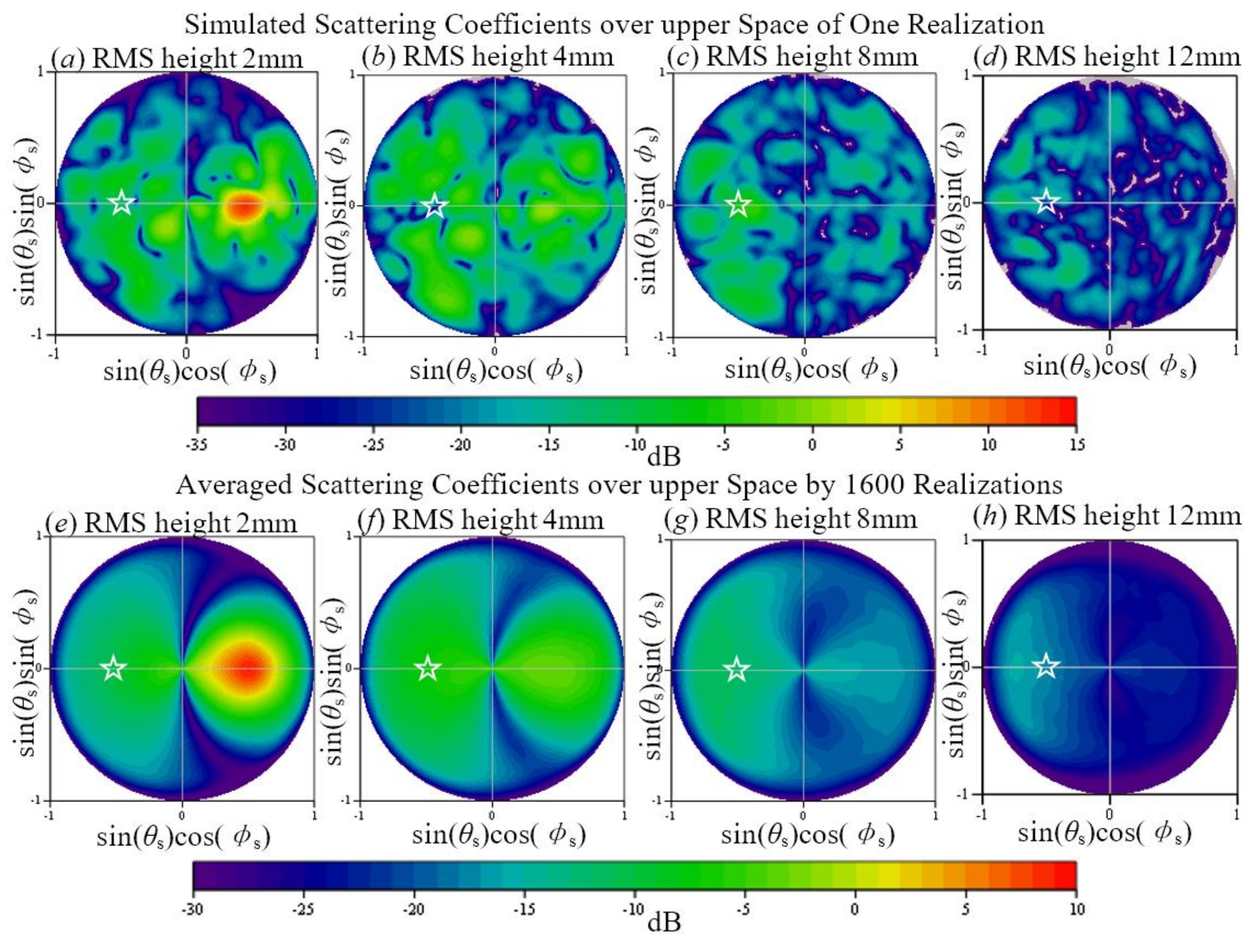
Figure 15, it is also interesting to observe that, as the h changes from 2 mm to 12 mm, the dominate bi-static scattering region gradually moves from the forward region (h = 2 mm) to the backward region (
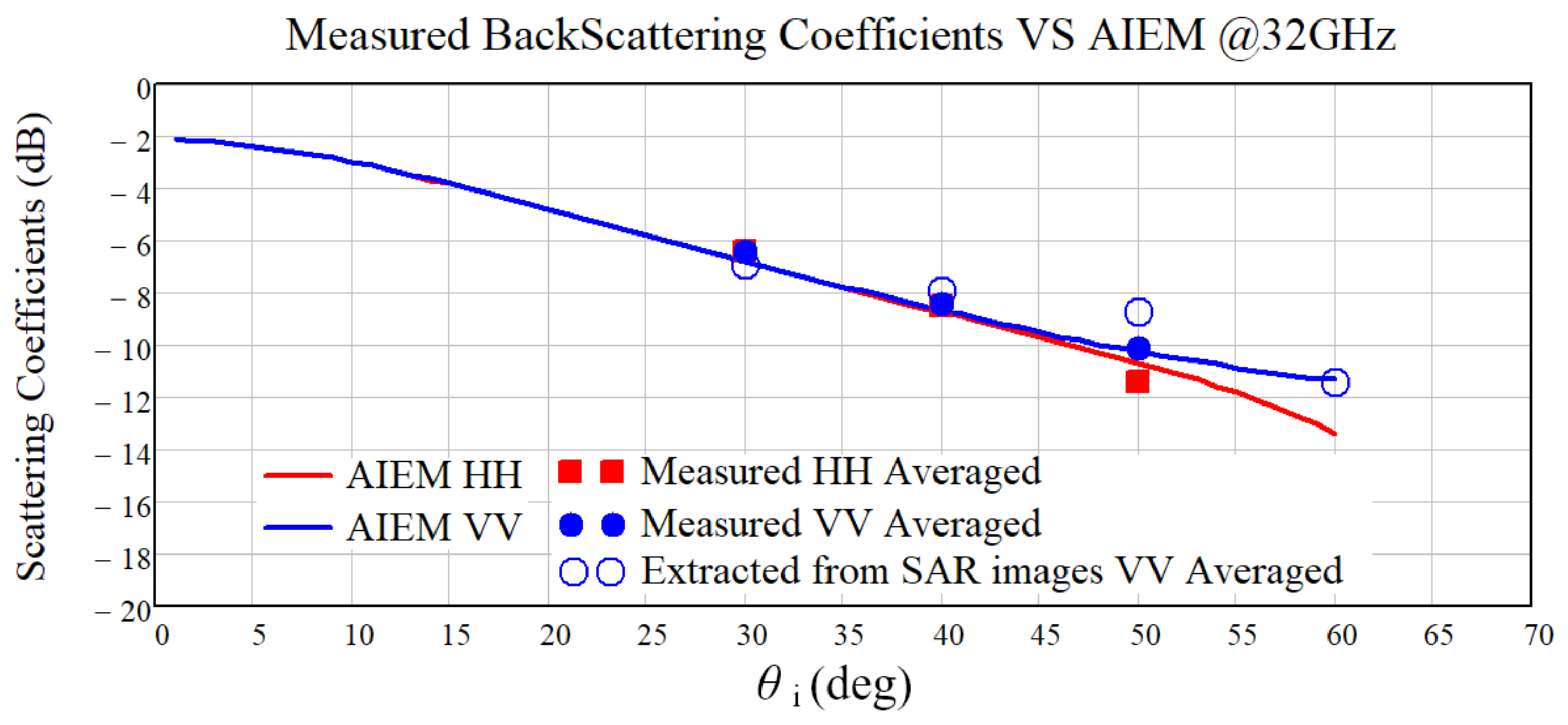
h = 12 mm). Also, the averaged computed backscattering coefficients are listed in Table 4 and a good agreement with the AIEM results can be observed.
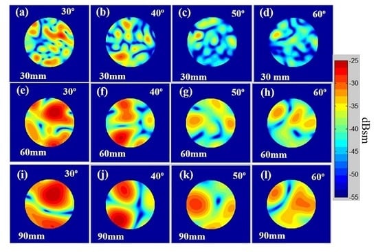
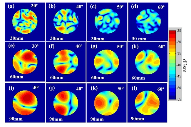
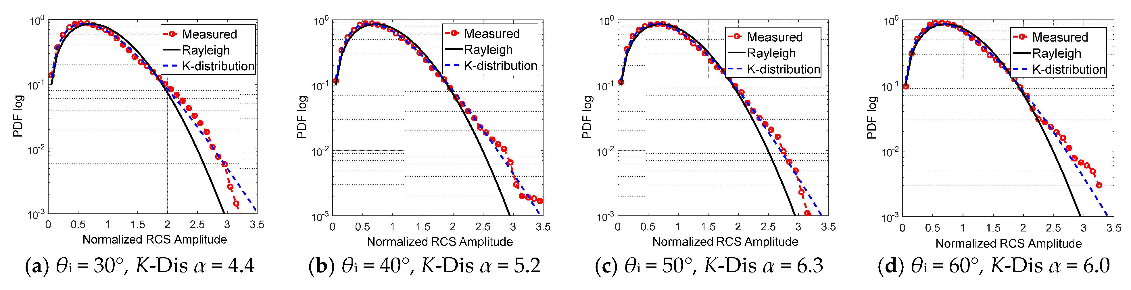
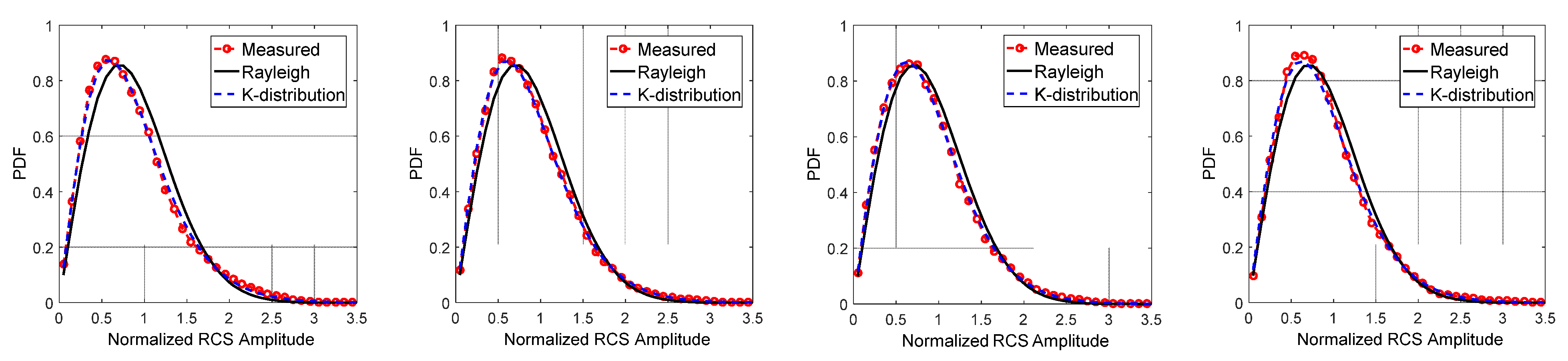
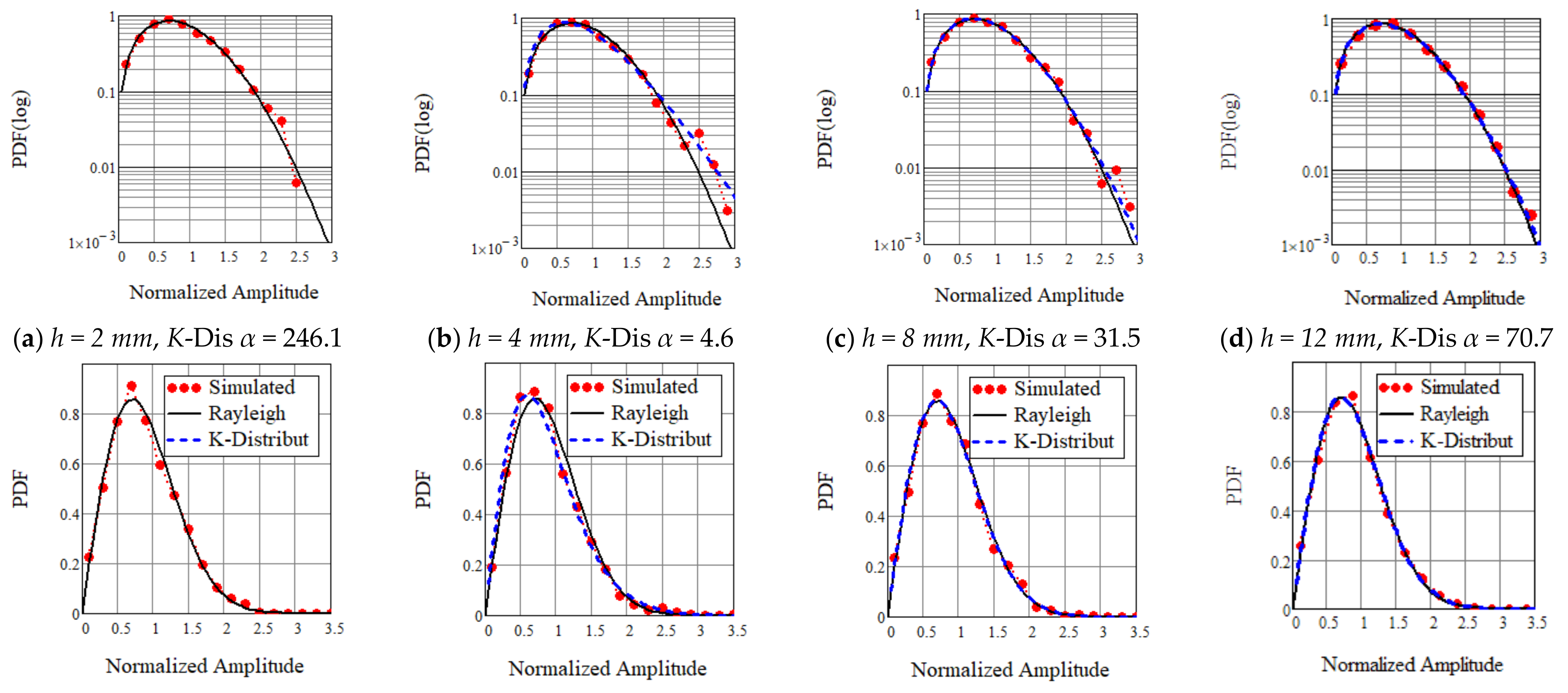
The computed amplitude speckle results are then presented in Figure 16 and Table 7, showing that: at the lowest and highest considered RMS height h values, the backscattering speckle amplitude PDF is very close to the Rayleigh distribution; meanwhile at the moderate h of 4 mm, the PDF is away from the Rayleigh one. The observed trends of speckle properties are interesting that it can be directly explained by neither the concept of equivalent number of scatterers, nor two scale scattering multiplicative process as the scattering scale factor. The equivalent number of scatterers theory predict that the N varies from several, to tens and then to thousands, as the RMS height changes from 2 mm to 12 mm, at the resolution level of 30 mm and θi = 30°. Keep in mind that the overall α is proportional to both the N and the statistical property of each independent scatters (αs), in the theoretic framework of equivalent number of scatterers. The rapid change of the estimated αs shown in the last line of Table 7 as the RMS h varies from 2 mm to 4 mm, is hard to be anticipated when using the equivalent number of scatters theory, if one does not consider other understandings on the scattering mechanisms. On the other hand, the long scale undulate gets more severe as the RMS height gets larger, the two scale multiplicative scattering process should be strengthened. It is also hard to understand that the counted α keeps getting larger as the RMS h varies from 4 mm to 12 mm (Table 7), if one only considers the explanation of the two scale multiplicative scattering process. Clearly, none of the two theories that produces monotonous trend prediction, can be independently used to explain the data results with such a non-monotonous trend.
Actually, it is most possible that both of the two effects should be considered in analyzing and further modeling the VHR speckle from exponentially correlated rough surface. When the RMS height is 2 mm, the slope of the rough surface is very small (0.042). Although the predicted equivalent number of scatterers within resolution cell size is small, those short-scale scatters remain a random Gaussian process without notable long-scale modulation. Therefore, with a large number of realizations (or return cells) the speckle remains the fully developed Rayleigh description. When the RMS height is 12 mm, the slope of the rough surface gets to 0.25, the process of long scale modulation of scattering from short-scale roughness should be notable. However, the equivalent scatterer number is too large (thousands) in this case; it is very likely that such a large number of scatters overwhelms the modulation effect, so that the VHR speckle is close to being fully developed again. Then it is worthy to get back to the case of h = 4 mm. One can found that, in this case, the scatterer number is moderate (tens) and not large enough, then the notable two-scale modulation effect drives the speckle PDF away from the Rayleigh distribution to the K-distribution with a moderate α.

5. Conclusions

In this work, the very high-resolution (VHR) speckle properties from exponentially correlated rough surfaces representing ground roughness is investigated by experimental measurements and numerical simulations. Both the equivalent scatterer number theory and scattering scale description of two scale multiplicative process can be found informative and perspective in analyzing the experimental and numerical results of VHR SAR images. However, by neither of them one can comprehensively explain the observed trends in the results. It is evident from the results that if the equivalent number of scatterers is not sufficiently large, the two-scale multiplicative scattering process may drive the VHR speckle PDF away from the fully developed Rayleigh description. Also, the dominance of a sufficiently large equivalent number of scatterers is also observed and that leads the VHR speckle properties close to the fully developed model even when the resolution cell size is smaller than the correlation length. It is confirmed that the equivalent number of scatterers may be useful in setting a bar for the VHR speckle modeling on exponentially correlated rough surfaces, below which the multiplicative scattering process should be considered and above that bar the Rayleigh model can be sufficient for modeling speckles.

Author Contributions

Conceptualization, M.J. and K.-S.C.; Methodology and Writing-Original Draft Preparation, M.J.; Investigation and Visualization, D.X.; Writing-Review & Editing and Funding Acquisition, K.-S.C.

Acknowledgments

This research was funded by the [National Science Foundation of China] grant number [41531175, 61701496], the Director General’s Innovative Funding-2015 from the institute of Remote Sensing and Digital Earth, CAS, as well as the [the State Key Laboratory of Remote Sensing Young Researcher Funds] grant number [16RC-03] from the State Key Laboratory of Remote Sensing Science. Also the authors appreciate Jungang Miao, Longzhao Qiao and Yulei Liu in the microwave engineering laboratory of Beihang University, for providing with the testing facilities and technique support.

Conflicts of Interest

The authors declare no conflict of interest.

References

  1. Ulaby, F.T.; Moore, R.K.; Fung, A.K. Microwave Remote Sensing: Active and Passive; Addison-Wesley: Reading, MA, USA, 1981. [Google Scholar]
  2. Tsang, L.; Kong, J.A.; Ding, K.H. Scattering of Electromagnetic Waves: Theories and Applications; John Wiley & Sons: New York, NY, USA, 2000. [Google Scholar]
  3. Lee, J.S.; Pottier, E. Polarimetric Radar Imaging: From Basics to Applications; CRC Press: Boca Raton, FL, USA, 2009. [Google Scholar]
  4. Chen, K.S.; Tsang, L.; Chen, K.L.; Liao, T.H.; Lee, J.S. Polarimetric simulations of SAR at L-Band over bare soil using scattering matrices of random rough surfaces from numerical three-dimensional solutions of Maxwell equations. IEEE Trans. Geosci. Remote Sens. 2014, 52, 7048–7058. [Google Scholar] [CrossRef]
  5. Jakeman, E.; Pusey, P.N. A model for non-Rayleigh sea echo. IEEE Trans. Antennas Propag. 1976, 24, 806–814. [Google Scholar] [CrossRef]
  6. Jakeman, E. On the statistics of K-distributed noise. J. Phys. A Math. Gen. 1980, 13, 31–48. [Google Scholar] [CrossRef]
  7. Sarabandi, K.; Oh, Y. Effect of antenna footprint on the statistics of radar backscattering from random surfaces. In Proceedings of the IEEE IGARSS, Firenze, Italy, 10–14 July 1995; pp. 927–929. [Google Scholar]
  8. Allain, S.; Ferro-Famil, L.; Pottier, E.; Fortuny, J. Influence of resolution cell size for surface parameter retrieval from polarimetric SAR data. In Proceedings of the IEEE IGARSS, Toulouse, France, 21–25 July 2003; pp. 440–442. [Google Scholar]
  9. Park, S.E.; Ferro-Famil, L.; Allain, S.; Pottier, E. Surface roughness and microwave surface scattering of high-resolution imaging radar. IEEE Geosci. Remote Sens. Lett. 2015, 12, 756–760. [Google Scholar] [CrossRef]
  10. Nesti, G.; Fortuny, J.; Sieber, A.J. Comparison of backscattered signal statistics as derived from indoor scatterometric and SAR experiments. IEEE Trans. Geosci. Remote Sens. 1996, 34, 1074–1083. [Google Scholar] [CrossRef]
  11. Di Martino, G.; Iodice, A.; Riccio, D.; Ruello, G. Equivalent number of scatterers for sar speckle modeling. IEEE Trans. Geosci. Remote Sens. 2014, 52, 2555–2564. [Google Scholar] [CrossRef]
  12. Ward, K.D.; Tough, R.J.A.; Watts, S. Sea Clutter: Scattering, the K Distribution and Radar Performance; IET: London, UK, 2006; pp. 106–112. [Google Scholar]
  13. Valenzuela, G.R. Theories for the interaction of electromagnetic and oceanic waves—A review. Bound. Layer Meteorol. 1978, 13, 61–85. [Google Scholar] [CrossRef]
  14. Rabus, B.; Wehn, H.; Nolan, M. The importance of soil moisture and soil structure for insar phase and backscatter, as determined by fdtd modeling. IEEE Trans. Geosci. Remote Sens. 2010, 48, 2421–2429. [Google Scholar] [CrossRef]
  15. Giannakis, I.; Giannopoulos, A.; Warren, C. A realistic FDTD numerical modeling framework of ground penetrating radar for landmine detection. IEEE J. Sel. Top. Appl. Earth Obs. Remote Sens. 2016, 9, 37–51. [Google Scholar] [CrossRef]
  16. Bai, M.; Jin, M.; Ou, N.; Miao, J. On scattering from an array of absorptive material coated cones by the PWS approach. IEEE Trans. Antennas Propag. 2013, 61, 3216–3224. [Google Scholar] [CrossRef]
  17. Chen, K.S.; Wu, T.D.; Tsang, L.; Li, Q.; Shi, J.C.; Fung, A.K. Emission of rough surfaces calculated by the integral equation method with comparison to three-dimensional moment method simulations. IEEE Trans. Geosci. Remote Sens. 2003, 41, 90–101. [Google Scholar] [CrossRef]
  18. Fung, A.K.; Chen, K.S. An Update on the IEM Surface Backscattering Model. IEEE Geosci. Remote Sens. Lett. 2004, 1, 75–77. [Google Scholar] [CrossRef]
  19. Zeng, J.Y.; Chen, K.S.; Bi, H.Y.; Zhao, T.J.; Yang, X.F. A Comprehensive analysis of rough soil surface scattering and emission predicted by AIEM with comparison to numerical simulations and experimental measurements. IEEE Trans. Geosci. Remote Sens. 2016, 55, 1696–1708. [Google Scholar] [CrossRef]
  20. Nouguier, F.; Guérin, C.-A.; Chapron, B. Scattering from nonlinear gravity waves: The ‘Choppy Wave’ model. IEEE Trans. Geosci. Remote Sens. 2010, 48, 4184–4192. [Google Scholar] [CrossRef]
  21. Pinel, N.; Chapron, B.; Bourlier, C.; de Beaucoudrey, N.; Garello, R.; Ghaleb, A. Statistical analysis of real aperture radar field backscattered from sea surfaces under moderate winds by Monte Carlo simulations. IEEE Trans. Geosci. Remote Sens. 2014, 52, 6459–6470. [Google Scholar] [CrossRef]
  22. Durden, S.L.; Vesecky, J.F. A physical radar cross-section model for a wind-driven sea with swell. IEEE J. Ocean. Eng. 1985, 10, 445–451. [Google Scholar] [CrossRef]
  23. Durden, S.L.; Vesecky, J.F. A numerical study of the separation wavenumber in the two-scale scattering approximation (ocean surface radar backscatter). IEEE Trans. Geosci. Remote Sens. 1990, 28, 271–272. [Google Scholar] [CrossRef]
  24. Fung, A.K. Backscattering from Multiscale Rough Surfaces with Application to Wind Scatterometry; Artech House: Norwood, MA, USA, 2015; pp. 3–4, 29–42. [Google Scholar]
Figure 1. Surface roughness spectrum of the considered rough surface samples at 32 GHz (k0 = 2π/λ). (Exponentially correlated rough surface, correlation length l of 48 mm).
Remotesensing 10 01369 g001
Figure 2. Geometry Configuration of the 3D model and the fabricated sample of the exponentially correlated rough surface. (a): CAD model; (b): Fabricated sample.
Remotesensing 10 01369 g002
Figure 3. Configuration of the indoor imaging measurement (sketch and photo). The 3 small spheres were utilized to compensate the antenna pattern effect.
Remotesensing 10 01369 g003
Figure 4. Image and range profiles of 3 small metal balls, showing the non-uniform illumination due to the antenna pattern effect. (a): Image profile; (b): Range profile (Two cut lines were obtained by performing 180° rotation of φ in the measurements).
Remotesensing 10 01369 g004
Figure 5. Configuration of FDTD simulations for rough surface scattering (The presented profile is one of the realization conducted in the numerical simulations).
Remotesensing 10 01369 g005
Figure 6. Comparison between measured scattering coefficients (σ0) of the exponentially correlated rough surface sample and the results by AIEM prediction, at 32 GHz. (The image extracted σ0 are from the image results of 60 mm resolution cell size and are also listed in Table 4).
Remotesensing 10 01369 g006
Figure 7. Comparisons between FDTD simulated upper-space bi-static scattering coefficients (σ0) and AIEM results, VV, 32 GHz, exponentially correlated rough surface, relative permittivity: 6.22-2.86j; (a) and (b): correlation length l = 48 mm, RMS height h = 4 mm; (c) and (d): l = 24 mm, h = 2 mm.
Remotesensing 10 01369 g007
Figure 8. Image example of the exponentially correlated rough surface sample at different resolutions (30 mm, 60 mm and 90 mm) and different θi (30°, 40°, 50° and 60°), VV.
Remotesensing 10 01369 g008
Figure 9. The normalized amplitude PDF curves of measured images at different θi, at the resolution cell size of 30 mm, VV, compared with Rayleigh distribution and K-distribution. (Sample parameters are shown in Table 1).
Remotesensing 10 01369 g009aRemotesensing 10 01369 g009b
Figure 10. The normalized amplitude PDF curves of measured images at different θi, at the resolution cell size of 60 mm, VV, compared with Rayleigh distribution and K-distribution. (Sample parameters are shown in Table 1).
Remotesensing 10 01369 g010
Figure 11. The computed γ value versus resolution cell size in case of different θi from the measured images, VV. “No Ant Correction” denotes for the γ values from images without the antenna pattern correction procedure. (Sample parameters are shown in Table 1).
Remotesensing 10 01369 g011
Figure 12. Results of simulated bi-static scattering coefficients over the upper space, considering different incident angle θi. The backscattering angular position is marked by the white-lined star. Sample and computation parameters are in Table 1 and Table 3(set 1).
Remotesensing 10 01369 g012
Figure 13. PDF curves of FDTD-simulated backscattering amplitude at different θi, at the footprint size of 30 mm, VV, compared with referencing Rayleigh distribution and K-distribution, 1600 realizations. Sample and computation parameters are in Table 1 and Table 3(set 1).
Remotesensing 10 01369 g013
Figure 14. Recorded total field (E-Field, maximum normalized, real part) in the incident plane cut from the exponentially correlated rough surface simulation, θi = 30°. (a) h = 2 mm, (b) h = 4 mm, (c) h = 8 mm.
Remotesensing 10 01369 g014
Figure 15. Results of simulated bi-static scattering coefficients over the upper space, considering different RMS height (h). The backscattering angular position is marked by the white-lined star. Sample and computation parameters are in Table 1 and Table 3(set 2).
Remotesensing 10 01369 g015
Figure 16. PDF curves of FDTD-simulated backscattering amplitude at θi = 30°, considering exponentially correlated surface with different h, (a): h = 2 mm; (b): h = 4 mm; (c): h = 8 mm; (d): h = 12 mm. VV, compared with referencing Rayleigh distribution and K-distribution, 1600 realizations. Sample and computation parameters are in Table 1 and Table 3(set 2).
Remotesensing 10 01369 g016
Table 1. Parameters of the exponentially correlated rough surface samples.
Sizehl
Measured Sample250 mm in diameter4 mm48 mm
(in λ@32 GHz)26.7 in diameter0.4275.12
Numerical Samples125 mm × 125 mm2 mm, 4 mm, 8 mm, 12 mm48 mm
(in λ@32 GHz)13.3 × 13.30.214, 0.427, 0.854, 1.2815.12
Table 2. Imaging parameters for different resolution cell size (R = 1.4 m, ground range resolution, Kaiser windows (β = 2.5) applied in both domains).
Ground ResolutionCenter FrequencyAperture LengthBandwidth (GHz)
θi: 30°θi: 40°θi: 50°θi: 60°
30 × 30 mm232.0 GHz240 mm11.008.256.606.15
45 × 45 mm2160 mm7.355.504.404.10
60 × 60 mm2120 mm5.504.133.303.07
75 × 75 mm296 mm4.403.302.652.45
90 × 90 mm280 mm3.702.752.202.05
Table 3. Computational parameters for the FDTD simulations @32 GHz.
Set 13 dB Footprint Sizeds * (mm)Domain Size (Yee Cells +)Realization Numberθi (h = 4 mm)
30 mm in diameter0.3123400 × 400 × 180160030°, 40°, 50°
Set 23 dB Footprint Sizeds * (mm)Z Direction Size (Yee Cells)Realization Numberh (mm) θi = 30°
30 mm in diameter0.3123160, 180, 220, 28016002, 4, 8, 12
* ds denotes the discretizing interval in the computation domain. + Yee cell is the mesh cell in the FDTD.
Table 4. Comparisons of the average intensity values and amplitude speckle values from the measured images at the resolution cell size of 30 mm and 60 mm. (Sample parameters shown in Table 1).
Resolutionθi (deg)30405060
AIEM σ0 (dB)−6.8−8.6−10.4−11.3
30 mm × 30 mmAverage σRCS (dBsm)−37.5−39.3−41.4−43.9
Average σ0 (dB)−6.4−7.7−9.0−10.5
α for K-dis4.55.26.36.0
Computed γ0.5980.5760.5710.564
60 mm × 60 mmAverage σRCS (dBsm)−32.0−33.5−35.1−38.8
Average σ0 (dB)−6.9−7.9−8.7−11.4
α for K-dis8.217.431.213.0
Computed γ0.5620.5320.5340.555
Table 5. Comparisons of the average intensity values and amplitude speckle values from simulated backscattering results by 1600 realizations, at the footprint size of 30 mm, Sample and computation parameters are in Table 1 and Table 3(set 1).
θi (deg)304050
AIEM σ0 (dB)−6.8−8.6−10.4
Average σ0 (dB)−7.3−9.0−10.2
α for K-dis 4.67.433.4
Computed γ0.5600.5470.531
Table 6. Comparison of amplitude γ in the case of imaging resolution cell/footprint size of 30 mm, at different θi, from measured images and simulated backscattering. Sample and computation parameters are in Table 1 and Table 3(set 1).
Method/θi (deg)304050
Imaging Measurement0.5980.5760.571
Numerical Simulation0.5600.5470.531
Fully Developed Ref0.52270.52270.5227
Table 7. Comparisons of the average intensity values and amplitude speckle values from simulated backscattering results by 1600 realizations, at the footprint size of 30 mm (3.2λ, 0.63l), Sample and computation parameters are in Table 1 and Table 3(set 2).
RMS Height h2 mm4 mm8 mm12 mm
AIEM σ0 (dB)−10.4−6.8−11.8−18.2
Numerical σ0 (dB)−10.0−7.3−12.0−17.7
Amplitude γ0.5250.560.5350.528
α for K-dis246.14.631.570.7
ENS Prediction N *12.443.4719.93668
ENS Predicted αe *20.244.3472.0366.8
αs = α/N (sub-scatters)102.50.1060.040.019
*1 Equivalent number of scatterers is predicted using Equation (8). *2 αe = N*αs and assuming that αs = 0.1.

