Imaging Simulation for Synthetic Aperture Radar: A Full-Wave Approach


1
Department of Communication Engineering, National Central University, Taoyuan 32001, Taiwan
2
Institute of Remote Sensing and Digital Earth, Chinese Academy of Sciences, Beijing 100101, China
3
Department of Electrical Engineering, National Taipei University of Technology, Taipei 10608, Taiwan
*
Author to whom correspondence should be addressed.
Remote Sens. 2018, 10(9), 1404; https://doi.org/10.3390/rs10091404
Submission received: 19 July 2018
/
Revised: 5 August 2018
/
Accepted: 29 August 2018
/
Published: 3 September 2018
(This article belongs to the Special Issue Radar Imaging Theory, Techniques, and Applications)
Abstract
:Imaging simulation of synthetic aperture radar (SAR) is one of the potential tools in the field of remote sensing. The echo signal in imaging simulation based on the point target model cannot be linked to practical scenes due to the model being a simple mathematical form, stating only the synthetic process and lacking the physical process based on electromagnetic theory. In this paper, the full-wave method is applied to include the electromagnetic effects in raw data generation, and then a refined omega-K algorithm is used to perform image focusing. According to the proposed method, the focused images not only demonstrate the difference under dielectric constant variation but also present the diversified interaction among the targets with the spacing change. In addition, the images are simulated in different observation modes and bandwidths to provide a satisfactory reference for the design of system parameters. The simulation results from the full-wave method also compare well with chamber experiments. The simulation of SAR imaging based on a full-wave method offers more complete recovery of scattering information and is useful in designing future novel SAR systems and in speckle reduction analysis.
1. Introduction
In the field of remote sensing, synthetic aperture radar (SAR) images play an important role with wide applications [1,2,3,4,5,6,7,8,9,10,11,12,13,14,15,16,17,18,19,20] in recognizing and identifying geophysical phenomena on the earth, such as water, land, ice, man-made structures, and wind over the ocean. The SAR works by transmitting the electromagnetic waves and coherently receiving echo signals from the targets. Then, the SAR image is produced by matched filtering the echo signal that preserves the electromagnetic interactions about and among the targets. Because SAR is a complex system, imaging simulation is an efficient means for system design [3,8,11,13,17], testing of imaging focusing algorithms [8,9,10,12,13], mission planning, geo-referencing [14], and SAR data analysis and interpretation [15], among others. The current discussion on SAR imaging simulation [8,9,10,11,12,13,16,17,18,19,20] models the image pixel as a collection of point targets, an approximated physical model that in some ways simplifies the synthetic aperture process. However, the assumption lacks a complete physical process in view of electromagnetic theory and is thus unable to fully depict electromagnetic characteristics.
The physical optics (PO) approximation [21,22] is widely used to approximate the scattering field from electrically large, perfectly conducting (PEC) objects. This approximation consists of using ray tracing to estimate the field on a surface and then integrating that field over the surface to calculate the scattered field. However, the approximation ignores multiple scattering effects and does not completely describe the electromagnetic properties among targets. The Born approximation [2,23,24,25] is commonly used to calculate the scattering field to the first order, i.e., ignoring multiple scattering. In the inverse scattering problem under approximation, the scattering equation is linearized since the only unknown parameter is the object function. The linearity is normally attained by assuming that the scattering is weak, which means that the variations in the scattering medium superposed over the constant vacuum background are small, so that the scattered field can be considered a first-order perturbation of the incident field that propagates in free space with no obstructions. However, the deviation of the scattering field based on the Born approximation has preconditions; thus, this solution describes a single-scattering approximation in which the electromagnetic waves are scattered off the surface only and do not penetrate the target.
In light of full wave simulation, Liao [26] applied finite difference time-domain (FDTD) in characterizing the electromagnetic scattering from the ground surface and targets over-surface. The analyses of imaging performance were performed in numerical experiments. Liao [27] also utilized the FDTD method to generate the far-field responses to the realistic environment. Both single and multiple objects were discussed independently and the mutual interactions with the background were presented. Both the frequencies response and imaging results demonstrated the preserved scattering information among targets. The results confirm the advantage of the full wave method to present more realistic scattering characteristics for the radar targets. Inspired by these, the objective of this paper is to gain insight into the electromagnetic fields scattering process of imaging in SAR. The full-wave approach employs a parallelized method of moments (MoM) [28,29] solution to simulate the scattering responses from targets. It follows that the echo signals are coherently summed within the antenna beam over the synthetic aperture length. Then, a refined omega-K algorithm [10] is applied to perform SAR image focusing. Several types of dielectric material are investigated to resolve the scattering behavior from the variation in the dielectric constant. Both densely and coarsely spaced discrete targets are considered, in which multiple scatterings are analyzed from the focused images. Based on the optimization system design, monostatic and bistatic observation modes are also performed within the different observation angles. In addition, the influences of different bandwidths on scattering characteristics in focused images are discussed. The simulation of SAR imaging based on the full-wave solution provides the ability to fully describe the electromagnetic characteristics among targets in designing future SAR systems.
The organization of this paper is as follows. In the next section, a description starts from the electromagnetic theory and proceeds to image processing, including a link between the scattering field and echo signal. A focusing algorithm is also briefly introduced in Section 2. Imaging simulations with diverse information are presented in Section 3. In Section 4, six test runs for both numerical simulation and measurement are conducted and averaged. Finally, in Section 5, conclusions and future directions are addressed to close the paper.
2. Formula of the Echo Signal and Imaging Algorithm
2.1. Scattering Field of the Echo Signal
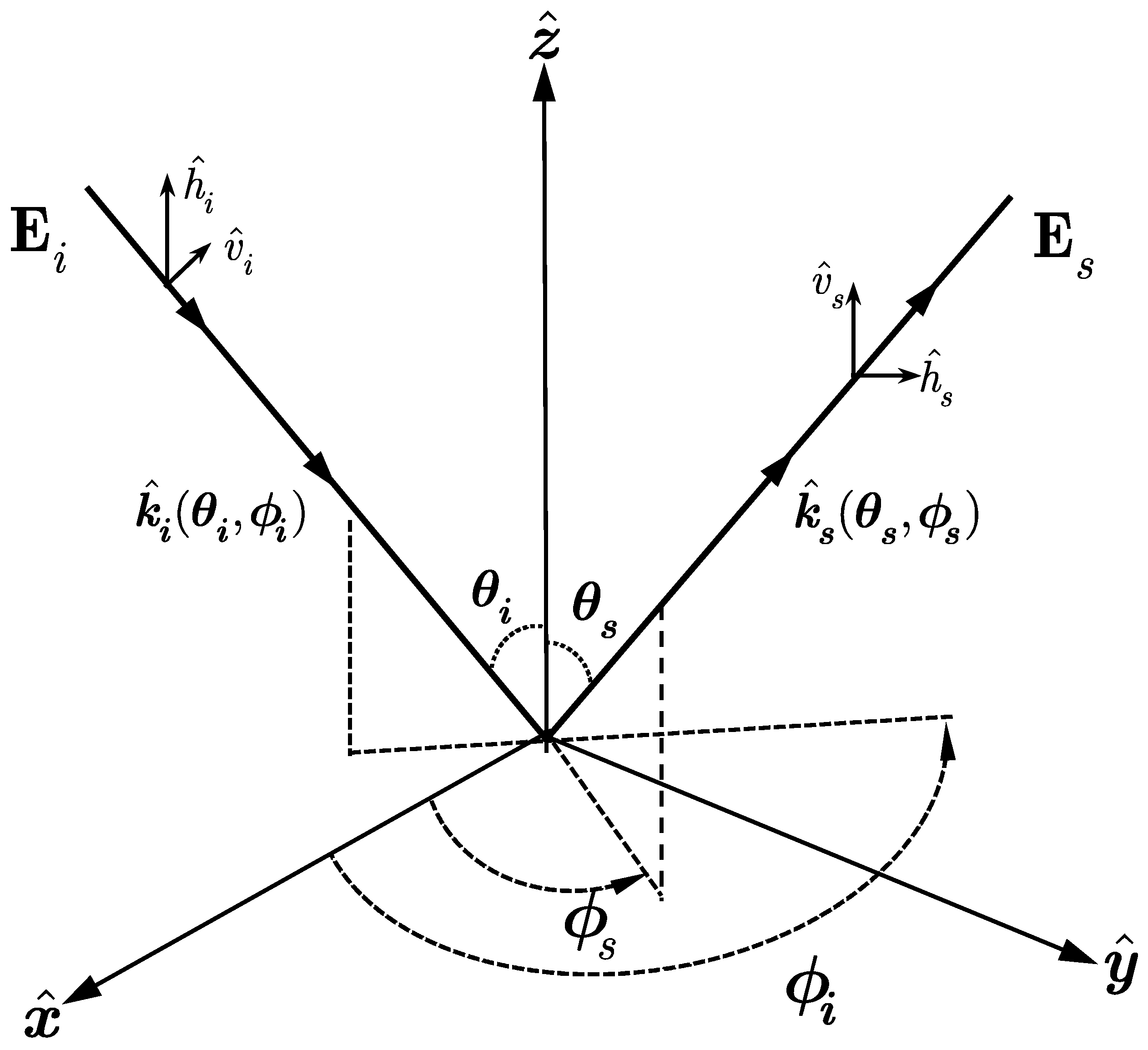
When an electromagnetic radar wave is incident upon targets, the scattering and propagation take place at the boundary between the two media [30,31,32]. Referring to the scattering geometry in Figure 1, the total electric field is
where is the incident field and is the scattered field. The volume integral equation (VIE) [13,29] governing the total field for a three-dimensional dielectric object is
where is the free space wavenumber, is the relative permittivity of the dielectric object, and is the electric dyadic Green’s function [30] in free space:
Numerical methods for solving the VIE in (2) have been well documented [28,29,32]. According to Maxwell’s equations, the surface currents are related to the total electric field as
where is the permittivity of the dielectric object and is the permittivity in free space.
The method of moments (MoM) is a general projection method for finding numerical solutions to linear (integral) operator equations. With the MoM, infinite dimensional integral equations are converted to a finite dimensional matrix equation. The surface current can be expanded via a sum of weighted basis functions .
where is a set of weights to be determined. RWG basis function is used in this paper. Galerkin method is then applied to convert the integro-differential equation, through Equations (1)–(5), into a matrix equation and the biconjugate gradient stabilized (BiCG-Stab) algorithm is utilized in solving the matrix equation to obtain . In particular, a maximum of 500 times or a residual error as low as is adopted to stop the iteration process in the BiCG-Stab operation. It follows that the surface current density (5) is readily obtained.
In synthetic aperture processing, the received signal from the scattered field is obtained by integrating the surface fields over an illumination area on the targets to gather two-dimensional data in the range (fast time ) and azimuth directions (slow time ). Suppose that the SAR system moves along the direction with velocity , we obtain the slant range varying with slow time:
Then, the time-harmonic scattered field received by SAR traveling along the y-direction, at far-field range , can be expressed as
where are surface fields given in Equation (5), with a two-dimensional Gaussian antenna gain pattern with full beam-width , centered at a resolution cell , is considered (see Figure 2).
In SAR [13], the received signal, called the echo signal, is a coherent sum of all scattered fields received at
where is the synthetic length (see Figure 2).
Note that for a linear frequency modulated (LFM) transmitting signal called chirp, a factor should be included, where is the chirp rate. The echo signal at this point remains a vector field. In receiving, if the antenna is -polarized, then we have
2.2. Image Focusing Algorithm
The SAR echo signal after demodulation [13] is
where is convolution operator; is the pulse duration, is the carrier frequency, is the anolog to digital conversion (ADC) sampling time or fast time, and is a rectangular function along the range direction:
is the antenna gain pattern, a function of slow time. The Gaussian antenna gain pattern is used in this paper. Now, taking the Fourier transform to the echo signal both in range and azimuth, we obtain
where is Fourier transform of Equation (9), and
Now that the matching filter is designed according to Equation (13). Several focusing algorithms have been proposed, including range-Doppler (RD), omega-K, and chirp-scaling, along with improved versions. The refined omega-K method [10] is used as a focusing algorithm in this paper because of its associated fast computation while maintaining suitable spatial resolution and small defocusing error. While the form varies between implementations, the omega-k algorithm requires a change of variables in the frequency domain referred to as Stolt mapping, named after the researcher who originally proposed the method for imaging the geological structure of the Earth. From the last term in Equation (14), the relevant portion of the frequency domain phase is
The phase term in Equation (14) includes the target phase due to the range encoding, range cell migration (RCM), range-azimuth coupling, and azimuth encoding.
The first focusing step is a reference function multiplication (RFM). The reference function is computed for a selected range. A target at the reference range is correctly focused by the RFM, but targets away from that range are only partially focused. Generally, the RFM is considered bulk compression.
After filtering by RFM, the phase remaining in the two-dimensional signal spectrum is approximately
Stolt mapping is the second focusing step to process the residual phase term. This process completes the focusing of targets away from the reference range by remapping the range frequency axis according to
To achieve perfect range compression and registration, the mapping transforms the original range frequency variable into a new range frequency variable , such that the phase is now linear in
TYheoretically, the range inverse Fourier transform (IFT) results in perfect range compression and registration. The mapping has effectively removed all the phase terms higher than the linear term and implements residual azimuth phase and range-azimuth coupling. For this reason, Stolt mapping can be viewed as differential compression. Finally, a two-dimensional IFT is performed to transform the data back to the time domain, i.e., the SAR image domain.
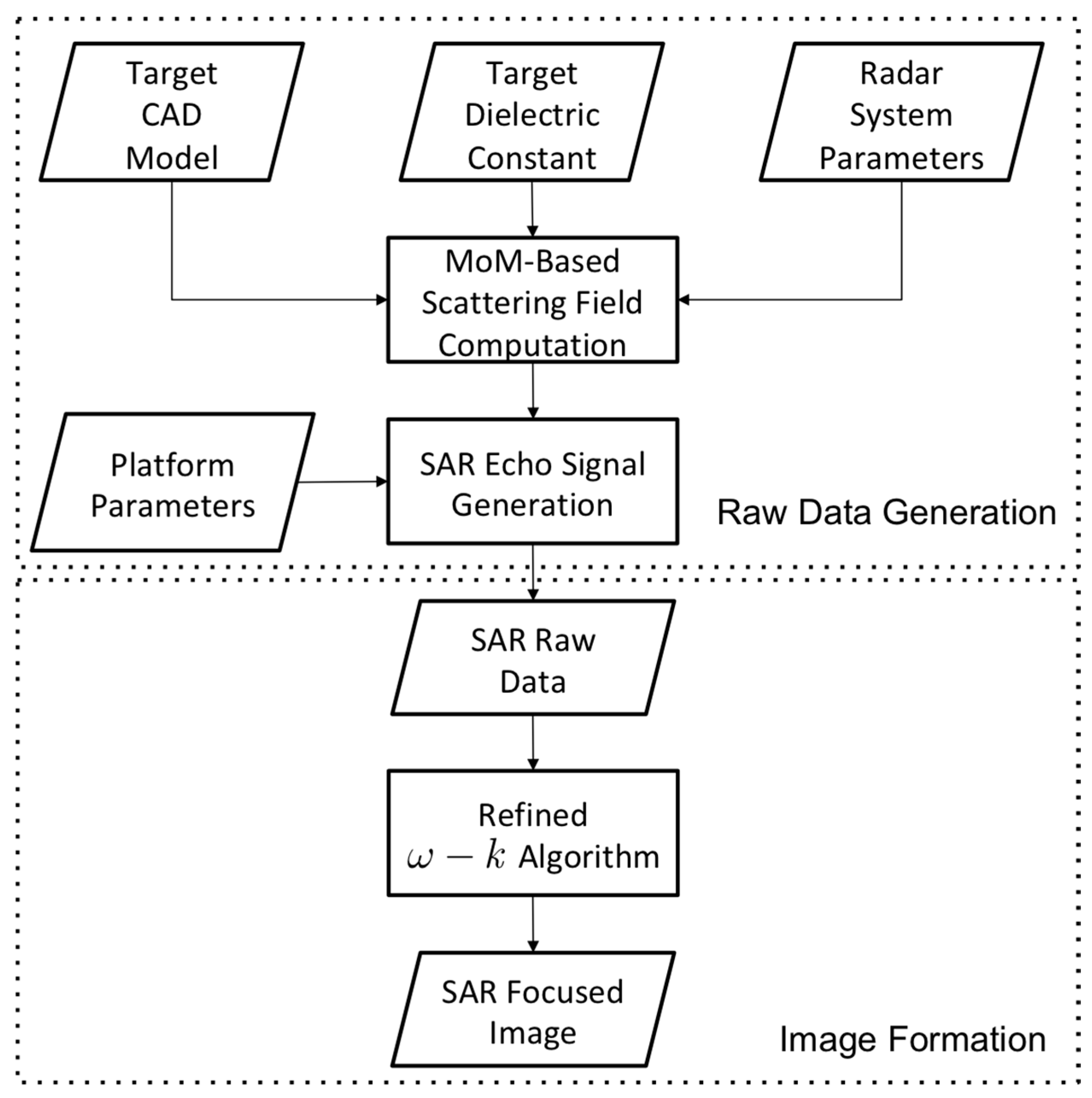
Figure 3 illustrates a functional block diagram of an SAR image simulation. The simulation processing flow is adopted from [13]. Generally, the inputs include the platform, radar parameter settings, and target CAD model. Then, the scattering fields are calculated within different platform positions, and the echo signal can be generated in two dimensions. An imaging algorithm is applied to achieve the final focused image.
3. Simulation Results
The numerical simulations are based on a practical experimental configuration with a total synthetic length of 1 m and a maximum slant range of 1.8 m. The system height from the ground plane is 1.5 m with a look angle of 45°. The antenna beam width is 17.5° from a typical standard gain horn antenna. The signal carrier frequency was set at 36.5 GHz with a 10 GHz bandwidth. Selected specifications are shown in Table 1.
A point-target model is a well-matched method for monostatic and bistatic system design, algorithm comparison and performance validation. However, the echo signal based on the model involves only the phase history rather than considering the physical properties of targets and does not fully present the complete electromagnetic behavior. In this study, a full-wave method is applied to generate the scattering field among targets and to make a physical link between it and the image formation. To evaluate the proposed method, the first simulation case is a single metal sphere, which is typically considered a reference target in the chamber experiment. An aluminum sphere (38,160,000 S/m) with a radius of 1.5 cm is placed at 1.1 m in the scene center. Both the results from the point-target model and the proposed method are shown in Figure 4.
The result in the proposed method shows the target location and considers the object size; the first target response in the focused image is at 1.085 m whereas the target center is at 1.1 m. According to the proposed method, creeping wave behavior is demonstrated in the range profile relative to a sinc-like target in the traditional imaging simulation. The location of the creeping wave appears at 1.15 m.
Without loss of generality, three different types of material, Teflon (relative permittivity and dielectric loss tangent ), glazed ceramic (relative permittivity and dielectic loss tangent ) and GaAs (relative permittivity and dielectric loss tangent ), are analyzed, and the results are shown in Figure 5. The white circle in the figures is the outline of the target, which is a sphere with 1.5 cm radius.
In the case of a single dielectric target, the rich information in the focused images is due to electromagnetic behavior such as scattering and penetration happening simultaneously. In the object with the lower dielectric constant, Teflon, most of the power penetrates through the media, so the first response is weak, whereas the multiple reflections are strong at the boundary with air on the other side of the target. With an increase in the dielectric constant, the first target response becomes stronger, demonstrating the true physical material properties in the focused images. Simultaneously, the delay peak moves backward because of the lower EM wave speed in the media. Different degrees of delays according to the dielectric constant are demonstrated as well. Table 2 shows the location of the peak delay both in the theoretical calculation and the simulation images.
In addition, the cases of multiple layer materials are analyzed with three different coating spheres. In these three spheres, the inner radius is 0.75 cm, and the materials are metal, glazed ceramic and GaAs. All the spheres are coated with 0.75 cm of Teflon. After raw data generation and imaging processing, the final focused images are presented in Figure 6. In the case of the metal sphere coated with Teflon, the scattering behavior presents as a single metal sphere, but the creeping wave phenomenon vanishes because of the coating layer. In the case of glazed ceramic coated with Teflon, only the first bounce and a single boundary reflection occur, and the penetration energy decreases rapidly. In the third case, because of the large difference in the dielectric constant, the scattering is dominated by the inner GaAs sphere.
In previous studies, simulated images using the point target model were calculated assuming that observation objects can be viewed as a superposition of multiple point targets. The result of two point targets under that assumption are shown in Figure 7. From the result, two targets are clearly identified, and the effect between them is the summation of the sinc function side lobe, in which no electromagnetic interaction is considered.
In the proposed method, simulations of metal, dielectric and coatings (metal coated with Teflon) for two targets are used to evaluate their interaction. Two spheres were separated along the azimuth direction, with spacing of 0 mm, 5 mm, 10 mm, 15 mm, 20 mm and 25 mm. The focused images in Figure 8 present the interaction among the targets. The case of two metal spheres features not only the two targets but also their mutual effects. The interactions are stronger with smaller displacement spacing and become weaker as the spacing increases. Due to the effects of transmission, scattering, and multi-path interactions, the results show more complex information in the dielectric object case. It is clear that multidelays are demonstrated in the range direction, which include the different levels of interactions with the spacing changes. In the case of coated spheres, only part of the power is scattered back because of the inner metal sphere. The level of interaction is weaker than for the pure metal targets. By testing different types of material, different degrees of interaction among targets can be analyzed in the simulations.
To further validate the proposed method, more complex targets in Figure 9 are simulated in three dimensions by three spheres (both the metal and dielectric) placed both along the range and azimuth directions with no spacing in the scene center. In the case of multiple targets, the interactions are weaker in the range than the azimuth direction. The different level of interactions in the azimuth direction is due to mutual effects among targets. The electromagnetic characteristics in the dielectric objects are more complex, and mutual interactions and self-interactions are shown at the same time. The different interaction degrees are illustrated that reduce target recognition ability. The results in Figure 9 highlight the difference between the point-target model and the proposed method.
SAR simulation could be a key to supplying system designers with possibilities that optimize radar components and assist in applications such as signal generation and analysis. The modular and flexible simulation structure allows adjustment and expansion for different tasks. SAR simulation tools are typically used to design SAR systems in the form of parametric studies that consider topics such as the prediction of image quality parameters. From the aspect of simulation, the system bandwidth is an important parameter in radar system design and is relative to the range resolution in the focused image. As the radar bandwidth increases, the electromagnetic interaction of a target can be resolved to varying degrees depending on the radar bandwidth. Hence, electromagnetic characteristics according to the variation in bandwidth in different materials are discussed. In the case of a single metal object, the radar bandwidth changes from 1 GHz to 10 GHz are shown in Figure 10. Because of single scattering behavior in a single metal target, the results show the bandwidth changing with little influence. Only the range resolution changes with the variation in bandwidth.
Next, three different types of material (namely, Teflon, glazed ceramic and GaAs) are used for analyzing the effect of bandwidth change for a single dielectric sphere. Due to the rich electromagnetic information in dielectric objects, the scattering effect based on system bandwidth is more pronounced. When the system bandwidth is small, the phenomenon of multiple scattering cannot be expressed because of the low range resolution. As the range resolution corresponds to the system bandwidth close to the size of the observation targets, the results show that one can make a distinction among different materials. In this study, when the system bandwidth reaches 5 GHz, that is, when the resolution is close to the object size level, the different target dielectric constants and the multiple scattering phenomenon can be illustrated in the various levels of results. The focused images presented in Figure 11 demonstrate that system bandwidth is profoundly significant for imaging dielectric objects relative to the metal targets.
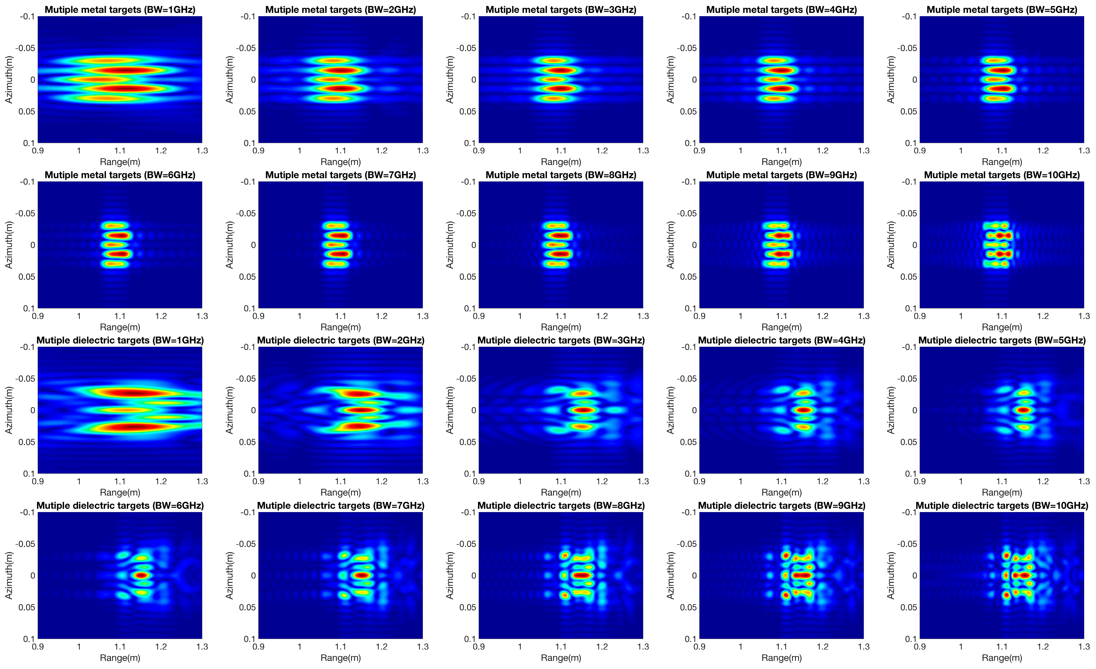
The effect of the system bandwidth on two targets is also discussed. Two different kinds of metal and dielectric objects are simulated with no spacing between targets. As shown in Figure 12, when the system bandwidth is lower, the ability to differentiate between metal and dielectric objects is poor, but their mutual interaction can still be illustrated. Moreover, the bandwidth changes only affect the resolution variation because of electromagnetic wave nonpenetration for the two metal objects. On the other hand, bandwidth alternations strongly affect the multipath imaging of a dielectric material. In addition, more complex objects are used for analysis of the system bandwidth. Both metal and dielectric materials with three-by-three spheres are placed along the range and azimuth directions with no spacing between objects. In the focused images of the metal spheres, the targets with mutual interaction in the azimuth direction can be clearly identified, and the targets in the distance image cannot be recognized as three objects because of lower resolution in the range direction. As the system bandwidth increases, the mutual interactions in the different levels are presented with the corresponding resolution. For the dielectric materials shown in Figure 13, different degrees of electromagnetic interaction are delivered with the variation in system bandwidth.
Whereas typical SAR imaging employs a collocated radar transmitter and receiver, as has been widely applied in the remote sensing field, limited pieces of information are extracted in specific angles from the monostatic system, which cannot fully present the target information. A bistatic SAR imaging system separates the transmitter and receiver to achieve benefits such as exploitation of additional information contained in the bistatic reflectivity of targets, increased radar cross section and increased bistatic SAR data information content with regard to feature extraction and classification. Currently, similar to the monostatic SAR simulation, the point-target is used in bistatic SAR imaging, which is an efficient way to develop and compare algorithms. However, this approach is unable to achieve the advantages of bistatic SAR to extract target information in different aspect angles. Hence, to evaluate the proposed method, the results both in monostatic and bistatic mode are simulated for the special case of equal velocity vectors for the transmitter and receiver. Figure 14 presents the different scattering behavior under the same system parameters with two directions of scattering azimuthal angles at 0 and 180 degrees.
Using the same system parameters with different observation angles, the intensity of the first bounce point in the bistatic results is the same as that in the monostatic: Increasing with increasing dielectric constant. However, the first bounce place moves backward in the bistatic simulation relative to the monostatic system. The effect of multiple scattering inside a sphere is significant in monostatic mode, but the behavior decays rapidly in bistatic mode. Moreover, it is clear that the location of multiple scattering moves forward in the bistatic system.
Two targets in bistatic mode are also simulated with two spheres separated along the azimuth direction with spacing of 0 mm, 5 mm, 10 mm, 15 mm, 20 mm, and 25 mm. The look angle is 45 degrees with azimuth angle at 0 and 180 degrees in two observation modes. The results in Figure 15 show the interaction between two targets in both monostatic and bistatic observations; diversified scattering information can be obtained through different observation angles. For the simulation results of the two objects, the intensity of mutual interaction is lower in bistatic mode than monostatic. However, the intensity of creeping waves is enhanced in the bistatic simulation over the monostatic system.
Two-by-two metal targets placed along the range and azimuth directions are shown in monostatic and bistatic modes in Figure 16. Two spheres are set with no spacing in the azimuth direction, and another two are five lambdas (0.0205 m) apart in the range direction. The monostatic case shows that original targets can still be identified with strong interaction in their centers. The interaction response is enhanced with the interaction in both the range and azimuth directions. As a result of the enhanced mutual interaction intensity, only the interaction is shown in the focused image, and the target recognition ability is reduced.
4. Experimental Results
To demonstrate the effectiveness and performance of the proposed method, we present results of numerical simulation and experimental measurement that were briefly outlined in the preceding section. The experiments are set in an anechoic chamber and two metal spheres are placed in the scene center with spacings of 0 mm, 5 mm, 10 mm, 15 mm, 20 mm and 25 mm. An N5224A PNA microwave network analyzer is used as a transmitter and receiver in this experiment. The system applies the motion controller to acquire data with a 1 cm interval in the total 1 m synthetic length. After collecting the raw data, focusing is carried out to obtain the focused images. In Figure 17, the results from the full-wave method compare well with the experimental results. The approach preserves the electromagnetic wave interactions between two spheres, and the interaction is reduced with spacing increases. Different degrees of interaction are present with the spacing variation between the targets, and the interaction intensity is reduced with increasing displacement.
5. Conclusions
In this paper, an SAR image simulation based on a full-wave approach is presented. By full-wave, the surface fields are able to preserve electromagnetic properties. By integrating the surface fields from different observation positions, we successfully establish a physical link between the scattering field and radar echo signal. Then, by applying an imaging algorithm, the focused SAR images based on the proposed method can be used to analyze the material properties and show the self- and mutual interactions among targets. Furthermore, system bandwidth and observation mode are discussed, thereby helping novel system design. To this end, it is suggested that more complex or even random targets should be explored for SAR simulated images based on a full-wave approach. Extension to more complex scenes in SAR image simulation seem highly desirable, as more of such data are available for much better system design capability, speckle reduction and further imaging algorithm development. In this aspect, further improvement of the computational efficiency by taking advantage of graphic processing unit (GPU) capability may be preferred and is subject to further analysis.
Author Contributions
C.-S.K. conceived the idea and designed and simulated the results; K.-S.C. conceived the concept and scheme; P.-C.C. verified and discussed the results; and Y.-L.C. guided the experiments.
Funding
This work was partially sponsored by the Ministry of Science and Technology of Taiwan under the Grants no. MOST 105-2221-E-027-120 and MOST-105-2116-M-027-001.
Conflicts of Interest
The authors declare no conflicts of interest.
References
- Tomiyasu, K. Tutorial Review of Synthetic-Aperture Radar (SAR) with Applications to Imaging of the Ocean Surface. Proc. IEEE 1978, 66, 563–583. [Google Scholar] [CrossRef]
- Ulaby, F.T.; Moore, R.K.; Fung, A.K. Microwave Remote Sensing: Active and Passive, Volume II, Radar Remote Sensing and Surface Scattering and Emission Theory; Artech House: Norwood, MA, USA, 1982; ISBN 13-978-0890061916. [Google Scholar]
- Curlander, J.C.; McDonough, R.N. Synthetic Aperture Radar: Systems and Signal Processing; Wiley-Interscience: New York, NY, USA, 1991; Volume 396, ISBN 13-978-0471857709. [Google Scholar]
- Henderson, F.M.; Lewis, A.J. Manual of Remote Sensing: Principles and Applications of Imaging Radar; Wiley: Hoboken, NJ, USA, 1998; Volume 2, p. 896. ISBN 978-0-471-29406-1. [Google Scholar]
- Elachi, C.; van Zyl, J. Introduction to the Physics and Techniques of Remote Sensing; John Wiley & Sons: Hoboken, NJ, USA, 2006; ISBN 13-978-0471475699. [Google Scholar]
- Lee, J.S.; Pottier, E. Polarimetric Radar Imaging: From Basics to Applications; CRC Press: Boca Raton, FL, USA, 2009. [Google Scholar]
- Moreira, A.; Prats-Iraola, P.; Younis, M.; Krieger, G.; Hajnsek, I.; Papathanassiou, K. A Tutorial on Synthetic Aperture Radar. IEEE Geosci. Remote Sens. Mag. 2013, 1, 6–43. [Google Scholar] [CrossRef] [Green Version]
- Carrara, W.G.; Goodman, R.S.; Majewski, R.M. Spotlight Synthetic Aperture Radar Signal Processing Algorithms; Artech House: Norwood, MA, USA, 1995; ISBN 13-978-0890067284. [Google Scholar]
- Franceschetti, G.; Lanari, R. Synthetic Aperture Radar Processing; CRC Press: Boca Raton, FL, USA, 1999. [Google Scholar]
- Cumming, I.; Wong, F. Digital Signal Processing of Synthetic Aperture Radar Data: Algorithms and Implementation; Artech House: Norwood, MA, USA, 2004. [Google Scholar]
- Oliver, C.; Quegan, S. Understanding Synthetic Aperture Radar Images; SciTech Publishing: Raleigh, NC, USA, 2004. [Google Scholar]
- Qiu, X.L.; Ding, C.B.; Hu, D.H. Bistatic SAR Data Processing Algorithms; Wiley: New York, NY, USA, 2013. [Google Scholar]
- Chen, K.S. Principles of Synthetic Aperture Radar: A System Simulation Approach; CRC Press: Boca Raton, FL, USA, 2015. [Google Scholar]
- Sheng, Y.; Alsdorf, D.E. Automated georeferencing and orthorectification of amazon basin-wide SAR mosaics using SRTM DEM data. IEEE Trans. Geosci. Remote Sens. 2005, 43, 1929–1940. [Google Scholar] [CrossRef]
- Gelautz, M.; Frick, H.; Raggam, J.; Burgstaller, J.; Leberl, F. SAR image simulation and analysis of alpine terrain. ISPRS J. Photogramm. Remote Sens. 1998, 53, 17–38. [Google Scholar] [CrossRef]
- Camporeale, C.; Galati, G. Digital computer simulation of synthetic aperture systems and images. Eur. Trans. Telecommun. Relat. Technol. 1991, 2, 343–352. [Google Scholar] [CrossRef]
- Franceschetti, G.; Migliaccio, M.; Riccio, D.; Schirinzi, G. SARAS: A synthetic aperture radar (SAR) raw signal simulator. IEEE Trans. Geosci. Remote Sens. 1992, 30, 110–123. [Google Scholar] [CrossRef]
- Gierull, C.; Ruppel, M. An end-to-end synthetic aperture radar simulator. In Proceedings of the EUSAR, Konigswinter, Germany, 26–28 March 1996; pp. 569–572. [Google Scholar]
- Meta, A.; Hoogeboom, P.; Ligthart, L.P. Signal processing for FMCW SAR. IEEE Trans. Geosci. Remote Sens. 2007, 45, 3519–3532. [Google Scholar] [CrossRef]
- Qiu, X.; Hu, D.; Zhou, L. A bistatic SAR raw data simulator based on inverse ω-k algorithm. IEEE Trans. Geosci. Remote Sens. 2010, 48, 1540–1547. [Google Scholar]
- Ling, H.; Chou, R.; Lee, S. Shooting and bouncing rays: Calculating the RCS of an arbitrarily shaped cavity. IEEE Trans. Antennas Propag. 1989, 37, 194–205. [Google Scholar] [CrossRef]
- Auer, S.; Hinz, S.; Bamler, R. Ray-tracing Simulation Techniques for Understanding High-resolution SAR Images. IEEE Trans. Geosci. Remote Sens. 2010, 48, 1445–1456. [Google Scholar] [CrossRef]
- Tsang, L.; Kong, J.A.; Shin, R.T. Theory of Microwave Remote Sensing; Artech House: Norwood, MA, USA, 1985; p. 627. [Google Scholar]
- Born, M.; Wolf, E. Principles of Optics: Electromagnetic Theory of Propagation, Interference and Diffraction of Light, 7th ed.; Cambridge University Press: Cambridge, UK, 1999. [Google Scholar]
- Gilman, M.; Tsynkov, S. A mathematical model for SAR imaging beyond the first born approximation. SIAM J. Imaging Sci. 2015, 8, 186–225. [Google Scholar] [CrossRef]
- Liao, D.H.; Dogaru, T. Full-Wave Scattering and Imaging Characterization of Realistic Trees for FOPEN Sensing. IEEE Geosci. Remote Sens. Lett. 2016, 13, 957–961. [Google Scholar] [CrossRef]
- Liao, D.H.; Dogaru, T.; Sullivan, A. Large-scale, full-wave-based emulation of step-frequency forward-looking radar imaging in rough terrain environments. Int. J. Sens. Imaging 2014, 15, 1–29. [Google Scholar] [CrossRef]
- Harrington, R. The Method of Moments in Electromagnetics. J. Electromagn. Waves Appl. 1987, 1, 181–200. [Google Scholar] [CrossRef]
- Gibson, W.C. The Method of Moments in Electromagnetics, 2nd ed.; CRC Press: Boca Raton, FL, USA, 2014. [Google Scholar]
- Ishmaru, A. Electromagnetic Wave Propagation, Radiation, and Scattering; Prentice-Hall: Upper Saddle River, NJ, USA, 1991. [Google Scholar]
- Chew, W.C. Waves and Fields in Inhomogeneous Media; Wiley-IEEE Press: Hoboken, NJ, USA, 1999. [Google Scholar]
- Tsang, L.; Kong, J.A.; Ding, K.H.; Ao, C.O. Scattering of Electromagnetic Waves, Vol. 2: Numerical Simulations; Wiley: New York, NY, USA, 2001. [Google Scholar]
Figure 1.
Scattering geometry with forward scattering alignment (FSA).

Figure 2.
Typical stripmap SAR observation geometry.

Figure 3.
Full-wave based SAR image simulation flowcharts.

Figure 4.
Comparison of focused images between the point-target model and the proposed method: Top row (left: point-target model and right: proposed method); bottom row: range profile (left: point-target model; right: proposed method).
Figure 4.
Comparison of focused images between the point-target model and the proposed method: Top row (left: point-target model and right: proposed method); bottom row: range profile (left: point-target model; right: proposed method).

Figure 5.
Images of dielectric spheres (left: Teflon; center: glazed ceramic; right: GaAs).

Figure 6.
Images of a coated sphere (left: metal coated with Teflon; center: ceramic glaze coated with Teflon; right: GaAs coated with Teflon).
Figure 6.
Images of a coated sphere (left: metal coated with Teflon; center: ceramic glaze coated with Teflon; right: GaAs coated with Teflon).

Figure 7.
Image of two targets based on the point-target model.

Figure 8.
Images of metal sphere, dielectric sphere, and metal sphere coated with Teflon with a spacing of 0 mm, 5 mm, 10 mm, 15 mm, 20 mm and 25 mm. (Top row: metal, middle row: dielectric and bottom row: metal coated with Teflon).
Figure 8.
Images of metal sphere, dielectric sphere, and metal sphere coated with Teflon with a spacing of 0 mm, 5 mm, 10 mm, 15 mm, 20 mm and 25 mm. (Top row: metal, middle row: dielectric and bottom row: metal coated with Teflon).


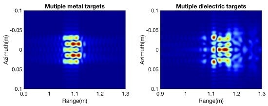
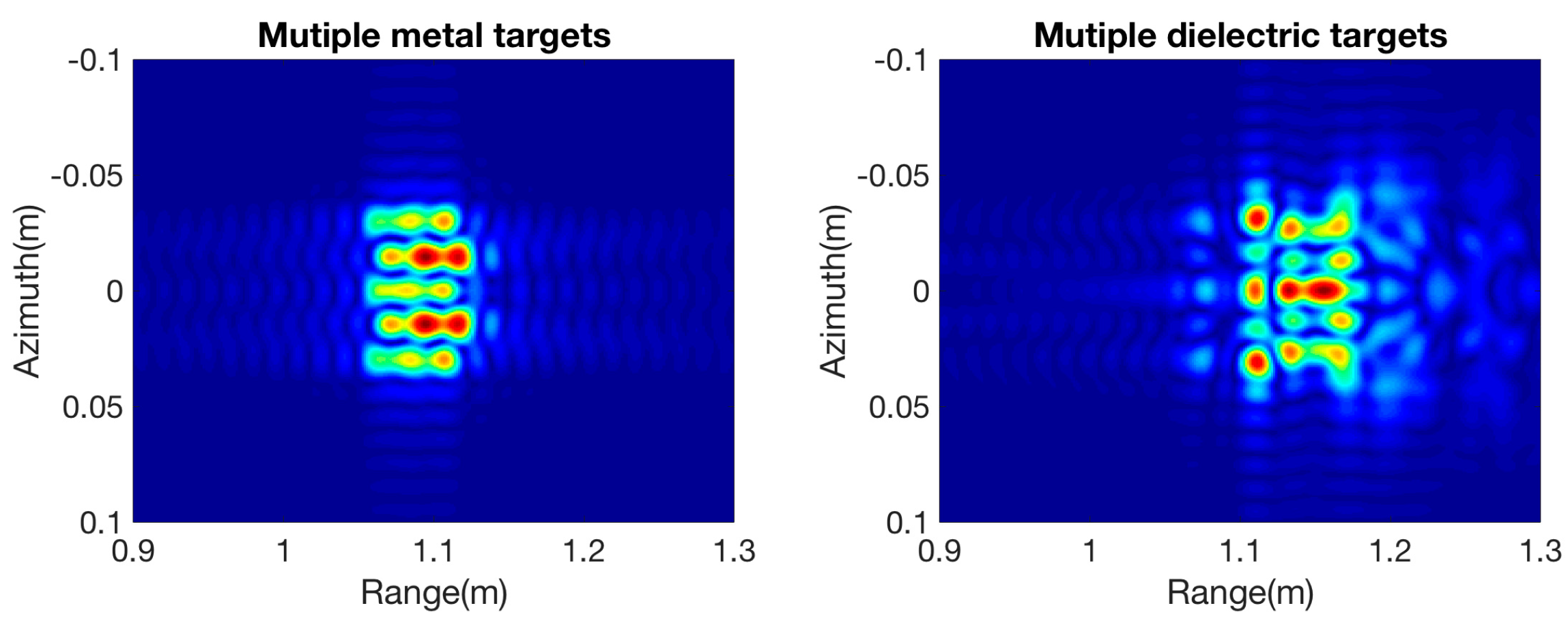
Figure 9.
Image of a cluster of three by three metal spheres (left) and dielectric spheres (right).

Figure 10.
Image of a metal sphere with SAR bandwidth varying from 1 GHz to 10 GHz.

Figure 11.
Images of a dielectric sphere with SAR bandwidth varying from 1 GHz to 10 GHz (top: Teflon; middle: glazed ceramic; bottom: GaAs).
Figure 11.
Images of a dielectric sphere with SAR bandwidth varying from 1 GHz to 10 GHz (top: Teflon; middle: glazed ceramic; bottom: GaAs).


Figure 12.
Image of two metal spheres (top two rows) and two dielectric spheres (bottom two rows) with SAR bandwidth varying from 1 GHz to 10 GHz.
Figure 12.
Image of two metal spheres (top two rows) and two dielectric spheres (bottom two rows) with SAR bandwidth varying from 1 GHz to 10 GHz.

Figure 13.
Images of a cluster of multiple metal spheres (top two rows) and dielectric spheres (bottom two rows) with SAR bandwidth varying from 1 GHz to 10 GHz.
Figure 13.
Images of a cluster of multiple metal spheres (top two rows) and dielectric spheres (bottom two rows) with SAR bandwidth varying from 1 GHz to 10 GHz.

Figure 14.
Image of a single dielectric sphere for the monostatic versus bistatic (left: Teflon; center: ceramic glaze; right: GaAs). (top row: monostatic; bottom row: bistatic).
Figure 14.
Image of a single dielectric sphere for the monostatic versus bistatic (left: Teflon; center: ceramic glaze; right: GaAs). (top row: monostatic; bottom row: bistatic).

Figure 15.
Case simulations of two metal spheres in the monostatic and bistatic modes with spacing of 0 mm, 5 mm, 10 mm, 15 mm, 20 mm and 25 mm. (top: monostatic and bottom: bistatic).
Figure 15.
Case simulations of two metal spheres in the monostatic and bistatic modes with spacing of 0 mm, 5 mm, 10 mm, 15 mm, 20 mm and 25 mm. (top: monostatic and bottom: bistatic).

Figure 16.
Images of a cluster of two by two metal spheres in backward and forward modes (left: monostatic; right: bistatic).
Figure 16.
Images of a cluster of two by two metal spheres in backward and forward modes (left: monostatic; right: bistatic).

Figure 17.
Images of two metal spheres (top row: simulated; bottom row: experimental) with spacing of 0 mm, 5 mm, 10 mm, 15 mm, 20 mm and 25 mm (from left to right).
Figure 17.
Images of two metal spheres (top row: simulated; bottom row: experimental) with spacing of 0 mm, 5 mm, 10 mm, 15 mm, 20 mm and 25 mm (from left to right).


Table 1.
Simulation parameters.
| Item | Value | Unit |
|---|---|---|
| Carrier Freq. | 36.5 | GHz |
| Bandwidth | 10 | GHz |
| Sensor Height | 1.5 | m |
| Target Location | 1.1 | m |
| Sensor Position Interval | 1 | cm |
| Look Angle | 45 | degree |
| Synthetic Length | 1 | m |
| Antenna Beam Width | 17.5 | degree |
| Sphere Radius | 1.5 | cm |
| Azimuth Angle (Incident) | 0 | degree |
| Azimuth Angle (Scattering) | 0 and 180 | degree |
| Scattering Angle (Bistatic) | 45 | degree |
Table 2.
Comparison between theoretical calculations and simulation results.
| Method | Teflon | Ceramic Glazed | GaAs |
|---|---|---|---|
| Theory | 1.1283 (m) | 1.1655 (m) | 1.1927 (m) |
| Simulation | 1.13 (m) | 1.165 (m) | 1.193 (m) |
© 2018 by the authors. Licensee MDPI, Basel, Switzerland. This article is an open access article distributed under the terms and conditions of the Creative Commons Attribution (CC BY) license (http://creativecommons.org/licenses/by/4.0/).
Share and Cite
MDPI and ACS Style
Ku, C.-S.; Chen, K.-S.; Chang, P.-C.; Chang, Y.-L. Imaging Simulation for Synthetic Aperture Radar: A Full-Wave Approach. Remote Sens. 2018, 10, 1404. https://doi.org/10.3390/rs10091404
AMA Style
Ku C-S, Chen K-S, Chang P-C, Chang Y-L. Imaging Simulation for Synthetic Aperture Radar: A Full-Wave Approach. Remote Sensing. 2018; 10(9):1404. https://doi.org/10.3390/rs10091404
Chicago/Turabian StyleKu, Chiung-Shen, Kun-Shan Chen, Pao-Chi Chang, and Yang-Lang Chang. 2018. "Imaging Simulation for Synthetic Aperture Radar: A Full-Wave Approach" Remote Sensing 10, no. 9: 1404. https://doi.org/10.3390/rs10091404
Note that from the first issue of 2016, this journal uses article numbers instead of page numbers. See further details here.