Article

“Regression-then-Fusion” or “Fusion-then-Regression”? A Theoretical Analysis for Generating High Spatiotemporal Resolution Land Surface Temperatures

State Key Laboratory of Earth Surface Processes and Resource Ecology, Faculty of Geographical Science, Beijing Normal University, Beijing 100875, China
*
Author to whom correspondence should be addressed.
Remote Sens. 2018, 10(9), 1382; https://doi.org/10.3390/rs10091382
Submission received: 27 July 2018 / Revised: 24 August 2018 / Accepted: 29 August 2018 / Published: 30 August 2018
(This article belongs to the Special Issue Remote Sensing Image Downscaling)

Abstract

:
The trade-off between spatial and temporal resolutions in satellite sensors has inspired the development of numerous thermal sharpening methods. Specifically, regression and spatiotemporal fusion are the two main strategies used to generate high-resolution land surface temperatures (LSTs). The regression method statically downscales coarse-resolution LSTs, whereas the spatiotemporal fusion method can dynamically downscale LSTs; however, the resolution of downscaled LSTs is limited by the availability of the fine-resolution LSTs. Few studies have combined these two methods to generate high spatiotemporal resolution LSTs. This study proposes two strategies for combining regression and fusion methods to generate high spatiotemporal resolution LSTs, namely, the “regression-then-fusion” (R-F) and “fusion-then-regression” (F-R) methods, and discusses the criteria used to determine which strategy is better. The R-F and F-R have several advantages: (1) they fully exploit the information in the available data on the visible and near infrared (VNIR) and thermal infrared (TIR) bands; (2) they downscale the LST time series to a finer resolution corresponding to that of VNIR data; and (3) they inherit high spatial reconstructions from the regression method and dynamic temporal reconveyance from the fusion method. The R-F and F-R were tested with different start times and target times using Landsat 8 and Advanced Spaceborne Thermal Emission and Reflection Radiometer data. The results showed that the R-F performed better than the F-R when the regression error at the start time was smaller than that at the target time, and vice versa.

Graphical Abstract

1. Introduction

Land surface temperature (LST) is a key parameter in environmental applications extending from local to global scales. This physical parameter is a key input of the surface energy balance model [1,2], which can be used to monitor evapotranspiration [3] and map land surface carbon [1]. In addition, LST is also used to study the urban thermal environment [4,5] and detect thermal anomalies before earthquakes [6].
Remotely sensed thermal images with high spatial and temporal resolution facilitate these environmental monitoring efforts. However, the available satellite thermal images yield a trade-off between spatial and temporal resolutions that limits the applications of LSTs. For example, thermal images of Landsat 8 or Advanced Spaceborne Thermal Emission and Reflection Radiometer (ASTER) have a spatial resolution of ~100 m but the repeat cycle is 16 days. In contrast, Moderate Resolution Imaging Spectroradiometer (MODIS) can generate 1 km-resolution LSTs four times per day. Thermal sharpening methods provide a solution to the resolution limitations.
The most widely used thermal sharpening method uses the relationship between LST and the normalized difference vegetation index (NDVI) to predict high-resolution LSTs [7], and it is efficient when used over a vegetated region. In addition to the NDVI, vegetation indices, such as the leaf area index, temperature vegetation dryness index, and ratio vegetation index, are also used as predictors to downscale LSTs [8]. To better adapt to an urban area, Dominguez developed the high resolution urban thermal sharpener (HUTS) to predict high-resolution LSTs using the relationship among the LST, NDVI, and surface albedo (α) [9]. In addition, the impervious surface index is applied in the disaggregation procedure for radiometric surface temperature (DisTrad) [7] and the TsHARP algorithm [10] to downscale urban LSTs as well [11,12]. These thermal sharpening methods are based on the assumption that the relationship between the LST and predictors is unique at different spatial resolutions [10]. Hence, we can obtain this relationship from low-resolution data and then predict high-resolution LST with the obtained relationship and predictors. These methods using predictors such as panchromatic images [13], emissivity [14], and surface albedo [9], can be considered as regression methods. Traditional regression tools, e.g., least-squares regression, build unique regression functions between LSTs and predictors [10]. However, when we use machine learning methods (e.g., artificial neural networks (ANN) [8], random forest (RF) [15], and support vector machine (SVM) [16]) as the regression tools, the details of the regression function are unknown. Specifically, compared with traditional regression tools, the RF regression yields better results and is more effective over heterogeneous regions [15,17], which indicates that the RF is a satisfactory regression tool for thermal sharpening.
Compared with the regression methods, which instantaneously downscale LSTs, spatiotemporal fusion methods use coarse/fine LST pairs to predict fine-resolution LSTs and thus can provide better data with high spatial and temporal resolution. Spatiotemporal fusion methods are different from traditional fusion methods, such as the intensity-hue-saturation (IHS) transformation [18], and wavelet decomposition [19,20], which combine high-resolution panchromatic data to obtain fine LSTs. For instance, the spatial and temporal adaptive reflectance fusion model (STARFM) [21] assumes that the land cover type and system error do not change over time. Combining details from neighboring pixels and temperature variation over time, the STARFM can effectively predict fine LST time series. The widely used STARFM has been the basis for many other spatiotemporal fusion methods, such as the unmixing-based, the weight function-based, and the dictionary-pair learning-based methods [22]. Limited in the pure temporal information obtained from the homogeneous pixels, the STARFM is less effective over heterogeneous regions [21]. Spatiotemporal fusion methods have been developed to solve the problems of the STARFM, such as the enhanced spatial and temporal adaptive reflectance fusion model (ESTARFM) [23], the spatio-temporal integrated temperature fusion model (STITFM) [24], and the spatio-temporal adaptive data fusion algorithm for temperature mapping (SADFAT) [25].
The aforementioned regression methods and the spatiotemporal fusion methods have their own advantages and disadvantages. Specifically, the regression methods downscale coarse LSTs to a fine resolution corresponding to the predictors obtained from the visible and near infrared (VNIR) bands. However, regression methods can only downscale LSTs instantaneously and have poorer performance when the ratio of the fine/coarse resolution is too large [26]. In addition, the spatiotemporal fusion methods can dynamically downscale LST time series but are limited by the resolution of the available fine LSTs. A combination of regression methods and spatiotemporal fusion methods is ideal to counteract their limitations and inherit their strengths. Bai [27] used an extreme learning machine (ELM) algorithm to downscale the Landsat ETM+ thermal infrared (TIR) data to a 30-m resolution then used the downscaled LST as input for the SADFAT to sharpen the MODIS LSTs. This method can be considered as the regression-then-fusion (R-F) method, i.e., using the regression method to first downscale the medium-resolution (~100 m) LST into fine resolution and then using the spatiotemporal fusion method to fuse the low-resolution LST time series and the downscaled LST obtained in the previous step. Accordingly, the fusion-then-regression (F-R) method, which has seldom been employed, uses the spatiotemporal fusion method to first fuse the low-resolution LSTs into medium resolution then downscales the fused medium-resolution LSTs into high-resolution via the regression method.
Because few studies have combined regression methods and spatiotemporal fusion methods together to generate high spatiotemporal LSTs, strategies for selecting from combinations of the two methods have not been discussed. The objective of this study is to present these two combinations (i.e., R-F and F-R) and discuss the strategies by which they have selected. The details of the two combinations and the strategies for selection are further described in Section 3. The results are tested and evaluated using the Landsat 8 data and ASTER data and are presented in Section 4. The discussion and conclusions are provided in Section 5 and Section 6, respectively.

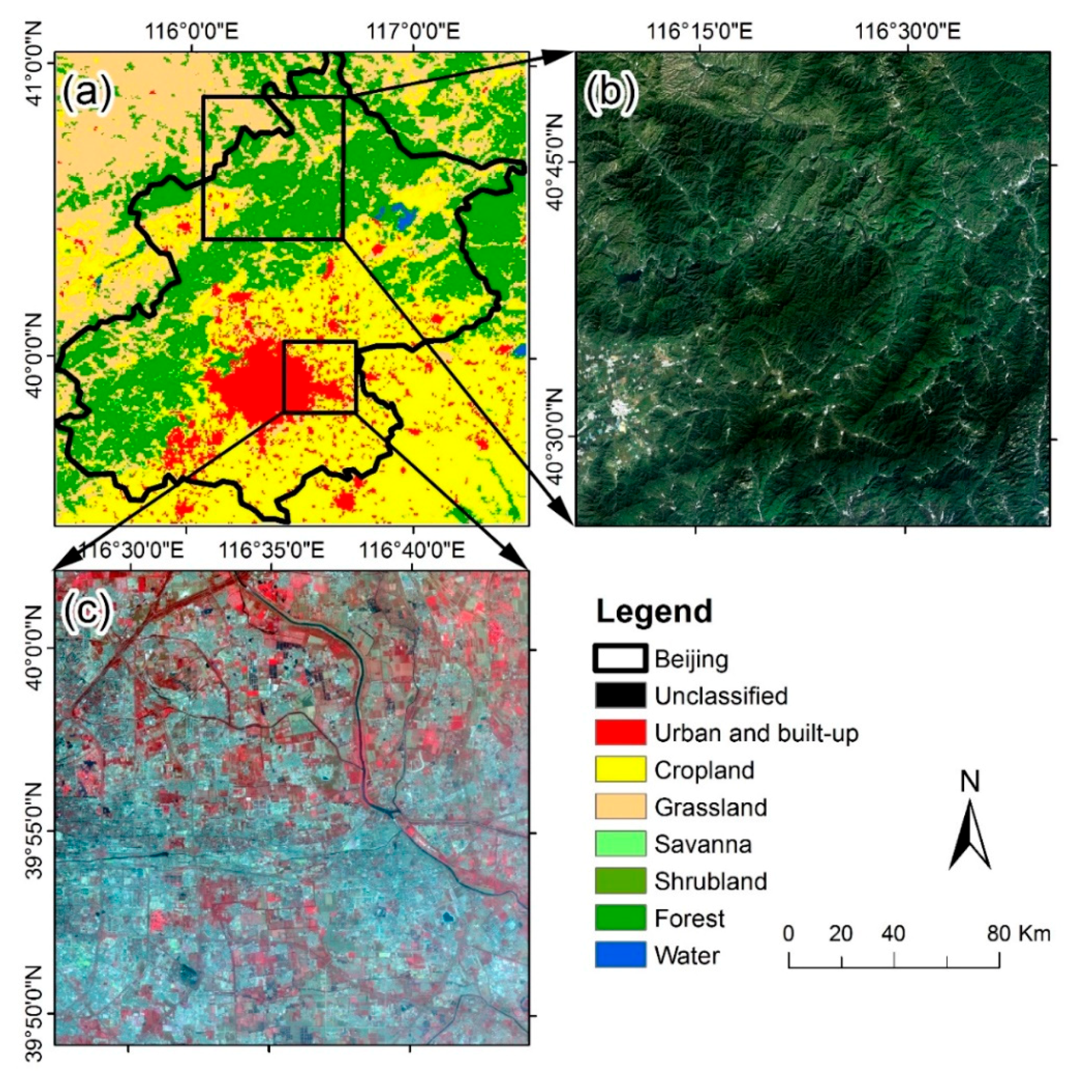
2. Data and Study Area

Landsat 8 datasets (downloaded from https://glovis.usgs.gov/) are used in this paper, of which the overpass time is approximately 10:50 local solar time. The thermal infrared (TIR) channel has a spatial resolution of 100 m, and the VNIR channel has a spatial resolution of 30 m. In addition, the LSTs are retrieved via a single channel algorithm using the TIR band 10 [28], of which the mean errors are below 1.5 K [28]. Landsat 8 datasets, collected on 4 September 2014 and 6 October 2014 with no clouds, are used for the predictions. The study area (see Figure 1b) is located in the north of Beijing and the land cover type is mainly forest and grassland, and it was selected because of its homogeneity.
ASTER data containing VNIR, short wave infrared (SWIR), and TIR channel are downloaded from https://glovis.usgs.gov/ and are used in Section 4. The spatial resolution is 15 m for the VNIR channel, 30 m for the SWIR channel, and 90 m for the TIR channel. We use the two-channel algorithms [29] to derive the LST, of which the accuracies are within 1.5 K [29]. Two ASTER TIR images under clear sky collected on 18 October 2004 (in the daytime and at night-time) and showing the same region (see Figure 1c) are used.

3. Methodology

This section first provides an overview of the regression and fusion methods (Section 3.1) and then presents the implementation details of the R-F and F-R methods (Section 3.2). Subsequently, we analyze the errors of the R-F and F-R method (Section 3.3) and then summarize the criteria used to determine the optimal strategy by comparing the errors of the R-F and F-R methods (Section 3.4). In addition, Section 3.5 introduces the implementation strategies with Landsat 8 data and ASTER data, respectively.

3.1. Overview of the Regression and Spatiotemporal Fusion Methods

3.1.1. Overview of the Regression Method

The regression method relies on the relationship between LST and predictors. The relationship is assumed to be invariant at different spatial resolutions [10]. Hence, the low-resolution LST and the corresponding predictors can be expressed as follow:
T l o w = f ( ρ l o w ) + ε l o w
where T l o w is the low-resolution LST, f ( · ) represents the function relationship between the LST and predictors, ρ l o w represents the low-resolution predictors, and ε l o w indicates the residual of the true LST and the predicted LST via f ( · ) at low resolution. Here, we apply the function relationship in the high-resolution data. The predicted LST at high resolution is obtained via the following equation:
T ^ h i g h = f ( ρ h i g h ) + ε l o w
where T ^ h i g h represents the predicted high-resolution LST, and ρ h i g h represents the high-resolution predictors.
Specifically, the function relationship is obtained using the regression tools, such as linear or non-linear regression [9,10], global or local regression, piecewise regression [30], and geographically weighted regression [31]. Since the RF regression has been satisfactorily tested in combination with a residual correction [15], we adopt the RF regression as the regression tool for this study. In addition, the reflectance of the VNIR channels is used as the predictors.

3.1.2. Overview of the Spatiotemporal Fusion Method

The spatiotemporal fusion method takes several fine LSTs and time series coarse LSTs to predict the fine LST time series. The STARFM, which requires minimum LST inputs, uses one fine LST and two coarse LSTs as inputs [21]. The similar pixels, which are determined using the spatial difference and temporal difference, are used to predict the fine LST. The equation used to predict the fine LST via the STARFM is given as follows:
T ^ h i g h   ( t 1 ) = T h i g h ( t 0 ) + k = 1 w W k × ( T l o w ( t 1 ) T l o w ( t 0 ) )
where t 0 is the start time, t 1 is the target time; T ^ h i g h ( t 1 ) is the predicted high-resolution LST at t 1 ; T h i g h ( t 0 ) represents the high-resolution LST at t 0 ; T l o w ( t 1 ) and T l o w ( t 0 ) represent the low-resolution LSTs at t 1 and t 0 , respectively; w indicates the number of the similar pixels within the moving window; and W k represents the weight that determines how much the similar pixels contribute to the central pixel. In addition, the similar pixels in a moving window are shown in Figure 2. The detailed principle for selecting the similar pixels is referenced in [21].

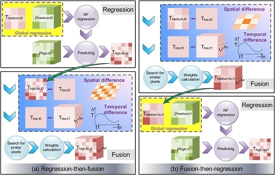
3.2. Implementations of the R-F and F-R Methods

The R-F and F-R methods are combinations of the regression and spatiotemporal fusion methods, and they downscale low-resolution LSTs into high-resolution LSTs based on the resolution of the VNIR data. Both regression and fusion methods involve two scales of resolution, i.e., low resolution and high resolution. However, in the R-F and F-R methods, we introduce the use of medium resolution. Hence, at least one medium-resolution LST at the start time and corresponding high-resolution VNIR data and two low-resolution LSTs at the start and target time are required in both strategies. For example, a 100 m resolution LST from Landsat 8 and corresponding 30 m resolution VNIR data and two 1 km resolution LSTs from MODIS can be used to generate 30 m diurnal LSTs via the R-F or F-R method. The implementation details of the R-F and F-R methods are shown in Figure 3, in which the notations correspond to the descriptions in Section 3.2.1 and Section 3.2.2.

3.2.1. Implementation Details of the R-F Method

The R-F method includes two steps (see Figure 3a). First, the medium-resolution LST and the corresponding VNIR data are used to obtain the regression relationship as follows:
T m e d i u m   ( t 0 ) = f m e d i u m , t 0 ( ρ m e d i u m ( t 0 ) ) + ε m e d i u m ( t 0 )
where T m e d i u m ( t 0 ) represents the medium-resolution LST at t 0 , ρ m e d i u m ( t 0 ) represents the predictors at t 0 , which is obtained from the VNIR data, f m e d i u m , t 0 ( · ) represents the relationship between T m e d i u m ( t 0 ) and ρ m e d i u m ( t 0 ) ; and ε m e d i u m ( t 0 ) indicates the residual between the true medium-resolution LST and the predicted medium-resolution LST via f m e d i u m , t 0 ( · ) at t 0 .
Here, we apply the relationship between high-resolution predictors to predict the high-resolution LST at t 0 using following equation:
T h i g h , r e   ( t 0 ) = f m e d i u m , t 0 ( ρ h i g h ( t 0 ) ) + ε m e d i u m ( t 0 )
where T h i g h , r e ( t 0 ) represents the predicted high-resolution LST via the regression method at t 0 and ρ h i g h ( t 0 ) represents the high-resolution predictors at t 0 . The regression method error can be expressed as follows:
ε h i g h , r e   ( t 0 ) = T h i g h , r e ( t 0 ) T h i g h ( t 0 )
We input the result of the regression method into the fusion method to obtain the high-resolution LST at the target time. The predicted fine LST is expressed as follows:
T h i g h , f u   ( t 1 ) = T h i g h , r e ( t 0 ) + k = 1 w W k × ( T l o w ( t 1 ) T l o w ( t 0 ) )
where T h i g h , f u ( t 1 ) indicates the predicted high-resolution LST via the fusion method at t 1 .

3.2.2. Implementation Details of the F-R Method

Similar to the R-F method, the F-R method includes two steps (see Figure 3b). First, a pair of medium-resolution and low-resolution LSTs at the start time and a low-resolution LST at the target time are used to obtain the medium-resolution LST at the target time. The predicted LST can be obtained using the following equation:
T m e d i u m , f u   ( t 1 ) = T m e d i u m ( t 0 ) + k = 1 w W k × ( T l o w ( t 1 ) T l o w ( t 0 ) )
where T m e d i u m , f u ( t 1 ) represents the predicted medium-resolution LST via the fusion method at t 1 .
We then use the results of the fusion method as input for the regression method to obtain the regression relationship between the LSTs and predictors as follow:
T m e d i u m , f u   ( t 1 ) = f m e d i u m , t 1 ( ρ m e d i u m ( t 1 ) ) + ε m e d i u m ( t 1 )
where ρ m e d i u m ( t 1 ) indicates the medium-resolution predictors at t 1 , f m e d i u m , t 1 ( · ) represents the relationship between T m e d i u m , f u ( t 1 ) and ρ m e d i u m ( t 1 ) , and ε m e d i u m ( t 1 ) indicates the residual between the fused medium-resolution LST and the predicted medium-resolution LST via f m e d i u m , t 1 ( · ) at t 1 .
We apply the regressed relationship to the high-resolution predictors, and the fine LST can be predicted using the following equation:
T h i g h , r e   ( t 1 ) = f m e d i u m , t 1 ( ρ h i g h ( t 1 ) ) + ε m e d i u m ( t 1 )
where T h i g h , r e ( t 1 ) represents the predicted high-resolution LST via the regression method at t 1 .

3.3. Error Analysis of the R-F and F-R Methods

3.3.1. Error Analysis of the R-F Method

The R-F method error is the difference between the predicted fine LST and the actual high-resolution LST at t 1 , which can be written as follows:
δ R F = T h i g h , f u ( t 1 ) T h i g h ( t 1 )
Combined with Equations (6) and (7), the R-F method error can be expressed as follows:
δ R F = T h i g h , r e ( t 0 ) + k = 1 w W k × ( T l o w ( t 1 ) T l o w ( t 0 ) ) T h i g h ( t 1 ) = T h i g h ( t 0 ) + ε h i g h , r e ( t 0 ) + k = 1 w W k × Δ T l o w T h i g h ( t 1 ) = Δ T m e d i u m Δ T h i g h + ε h i g h , r e ( t 0 )
where Δ T l o w = T l o w ( t 1 ) T l o w ( t 0 ) , Δ T m e d i u m = T m e d i u m ( t 1 ) T m e d i u m ( t 0 ) , and Δ T h i g h = T h i g h ( t 1 ) T h i g h ( t 0 ) . The R-F method error contains the errors caused by the regression process and the fusion process. Here, when we ignore the error caused by the fusion process, the error of the R-F method can be simplified as follows:
δ R F = ε h i g h , r e ( t 0 )

3.3.2. Error Analysis of the F-R Method

The F-R method error is the difference between the predicted fine LST and the true high-resolution LST at t 1 , which can be written as follows:
δ F R = T h i g h , r e ( t 1 ) T h i g h ( t 1 )
In addition, the regression method error at t 1 can be written as follows:
ε ^ h i g h , r e   ( t 1 ) = T h i g h , r e ( t 1 ) T h i g h ( t 1 )
This regressed error contains the error of the fusion process, since we use the fused result as the input in the regression process. Here, we assume the error of the fusion process is small enough to be ignored. Hence, the F-R method error can be simplified as follows:
δ F R   = ε h i g h , r e ( t 1 )
This regressed error is different to that in Equation (15) that does not contain the error of the fusion process.

3.4. Comparisons of the R-F and F-R Method Errors

The squared error (SE) [32] is used to describe the performance of the R-F and F-R methods. The SE of the predicted LST is expressed as follows:
SE = ( T p r e   T t r u e ) 2
where T p r e represents the predicted LST, and the T t r u e represents the actual LST. Hence, the error difference between the R-F and F-R is as follows:
S E R F S E F R = δ R F 2 δ F R 2
Combined with Equations (13) and (16), Equation (18) can be expressed as follows:
S E R F S E F R = ε h i g h , r e ( t 0 ) 2 ε h i g h , r e ( t 1 ) 2
Both R-F method error and F-R method error neglect the error of the fusion process, of which the difference is the resolution difference. Specifically, the fusion process of the R-F method sharpens the low-resolution LST into high resolution, while that of the F-R method sharpens the low-resolution LST into medium resolution. Therefore, when we compare the R-F method error and F-R method error, the fusion process error can be ignored when the fusion process error is almost undifferentiated at different downscaling ratios. Here, we compare the SEs of the R-F and F-R methods according to Equation (19). The SE of the R-F method is larger than that of the F-R method when the regression error satisfies Equation (20).
ε h i g h , r e   ( t 0 ) 2 > ε h i g h , r e ( t 1 ) 2
In contrary, the SE of the R-F method is smaller than that of the F-R method when the regression error satisfies Equation (21).
ε h i g h , r e   ( t 0 ) 2 < ε h i g h , r e ( t 1 ) 2
In conclusion, we obtain the criteria to determine which method is better: when the performance of the regression at t 0 is better than that at t 1 , the R-F method is better than the F-R method, and when the performance of the regression at t 1 is better than that at t 0 , the F-R method is the better choice.

3.5. Implementation Strategies with Landsat 8 Data and ASTER Data

We use the Landsat 8 data collected over two days to implement the R-F and F-R methods. One date is used as the start time data while the other is used as the target time. First, we aggregate the 100 m data (both LST and reflectance of the VNIR bands) to 300 m resolution as the medium-resolution data, and then the 300 m resolution LSTs are aggregated to 3 km as the low-resolution data. We then use the R-F and F-R methods to sharpen the low-resolution LST to high-resolution LST. The implementation details are shown in Figure 4. The results of step 1 are the products of the middle process. To evaluate the transmitted errors caused by step 1, we use the actual LSTs to generate 100 m resolution LSTs using the single regression method or fusion method. The original 100 m resolution LST is compared with the sharpened LSTs. Here, we also use the root mean square error (RMSE), mean absolute error (MAE), Pearson’s correlation coefficient (r), and Co-Occurrence Root Mean Square Error (CO-RMSE) [33] to evaluate the accuracy of the thermal sharpening methods.
We also use ASTER data collected in one day to implement the R-F and F-R methods. TIR data collected in the daytime is used as the start time data while that at night-time is used as the target time. First, we aggregate the 90 m data (both LST and reflectance of the VNIR bands) to 270 m resolution as the medium-resolution data, and then the 270 m resolution LSTs are aggregated to 2.7 km as the low-resolution data. We then use the R-F and F-R methods to sharpen the low-resolution LSTs. The implementation details are shown in Figure 5. Here, we have not analyzed the transmitted errors caused by step 1 using the single regression method or fusion method, because the implementation with ASTER data is intended to evaluate the performance of the F-R and R-F methods in one day.

4. Results

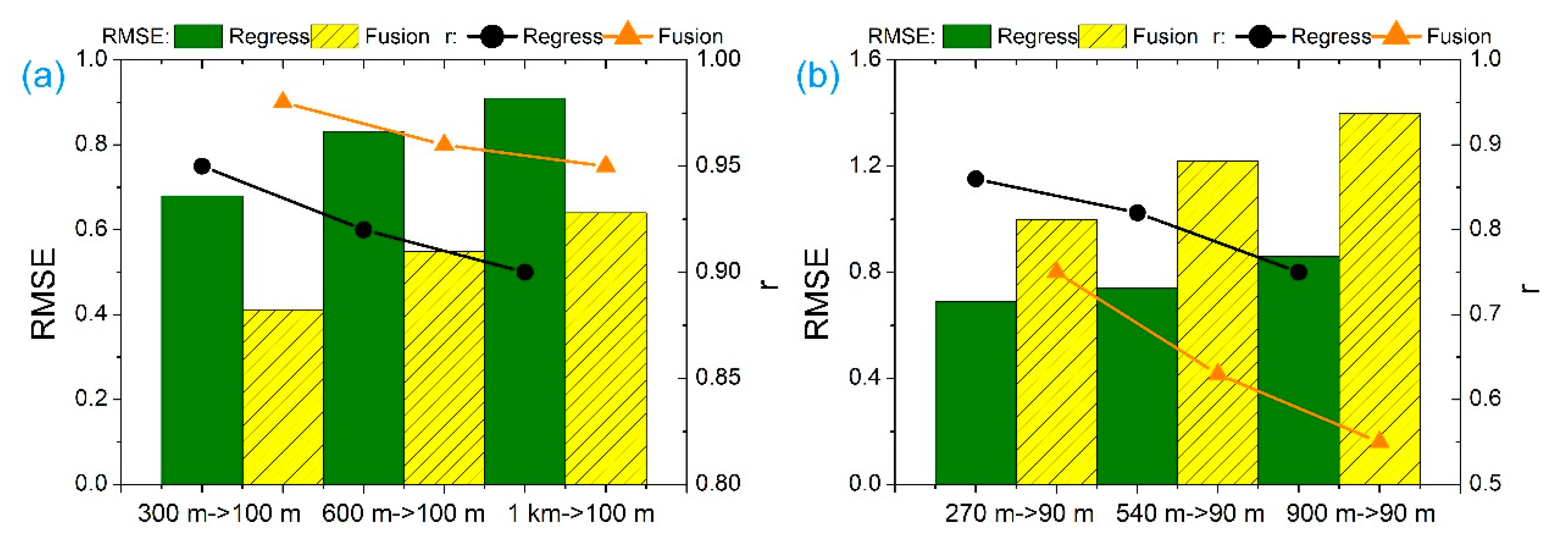
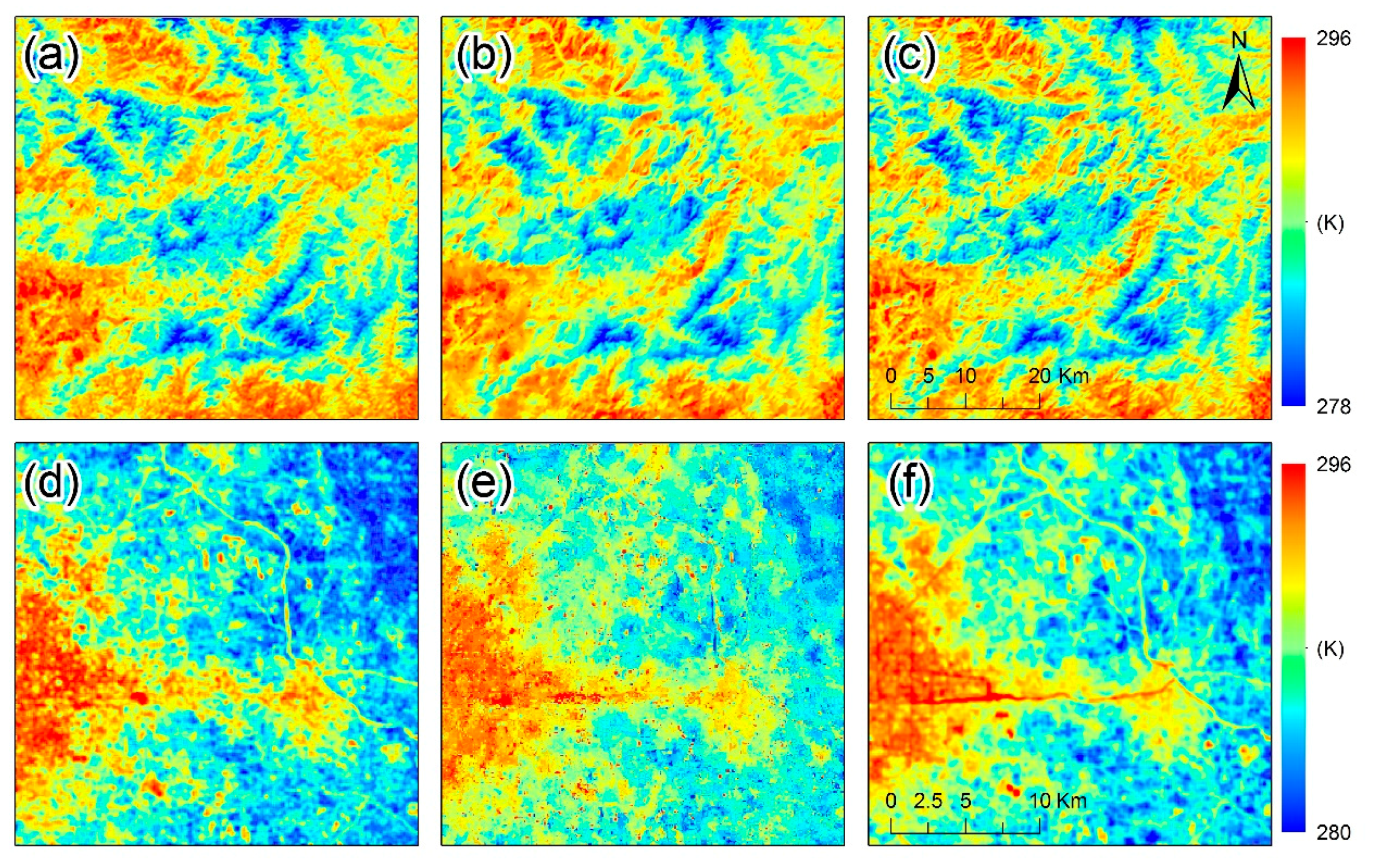
4.1. Tests with Landsat 8 Data on Different Days

4.1.1. Results of the R-F and F-R Methods When ε h i g h , r e ( t 0 ) 2 > ε h i g h , r e ( t 1 ) 2

Landsat 8 data collected over two days were used to implement the R-F and F-R methods. Specifically, data collected on 4 September 2014 were used as the start time data while data collected on 6 October 2014 were used as the target time data, because the error of the regressing process on 4 September 2014 was larger than that on 6 October 2014. The implementation details are introduced in Section 3.5.
The results of the sharpened LSTs are shown in Figure 6. A visual comparison shows that the results of the F-R method are better than that of the R-F method with more similar details to the actual LST. A quantitative comparison of the results in Figure 6g,h indicate that the F-R method performs better than the R-F method and presents lower RMSE, MAE, and CO-RMSE values and a higher r value. In addition, we also used the SEs to evaluate the F-R and R-F methods. As shown in Figure 7a,b, the spatial distribution of the difference between the regressed errors in two days along with the difference between the SEs of the R-F and of the F-R methods are similar. The similar spatial distribution illustrates that when the error of the regression method at the target time is smaller than that at the start time, the F-R method is better than the R-F method for sharpening the LST. That is because the larger difference of the regression errors between two different days indicates poorer performance of the regression method on 4 September 2014, and larger difference of the SEs indicates poorer performance of the R-F. In addition, the scatter plot representing the SEs of the R-F and F-R methods also shows a higher performance of the F-R method because more spots are located on the one-to-one dividing line (Figure 7c).
Since the results of the regression/fusion method are used as the input of the other method, errors transmitted during the middle process cannot be avoided. Here, we compared the accuracies of the F-R and R-F methods with that of the single method (i.e., regression/fusion method) to analyze the error propagation. As shown in Figure 8a, the accuracy of the F-R method (step 2) is lower than that of the middle process (step 1) and presents a higher RMSE value and a lower r value, which is partly due to the differences in scale that are applied in the two methods, namely, the fusion process downscaling the 3 km resolution LST to 300 m, and F-R downscaling the 300 m fused LST to 100 m. In addition, the F-R method takes the result of the fusion process as the input of the regression process, which means that the final result contains errors from both the fusion and regression methods. To analyze the performance of the transmitted error, we compared the accuracy of the F-R method with that of the regression method (contrast), which used the actual 300 m resolution LST for the regression. Compared with the regression method, the F-R method increased the RMSE value by 0.27 K, and decreased the r value by 0.05 (Figure 8a).
As for the R-F method, the error is larger than that of the middle process (step 1 in Figure 8b) because the error of the R-F method contains the error transmitted from the fusion process. In addition, compared with the fusion method (contrast), the R-F method increases the RMSE value by 0.15 K, and decreases the r value by 0.06 (Figure 8b). The increased error of the R-F method caused by the middle process is smaller than that of the F-R method, which means that the transmitted error in the F-R method impacts the final result more than that in the R-F method. However, the F-R method still has a higher performance than the R-F method when the error of the regression method is smaller at the target time than the start time.

4.1.2. Results of the R-F and F-R Methods When ε h i g h , r e ( t 0 ) 2 < ε h i g h , r e ( t 1 ) 2

Here, we used the same data as that in Section 4.1.1. However, the data collected on 6 October 2014 were used as the start time data, whereas the data collected on 4 September 2014 were used as the target time data. As shown in Figure 9, the spatial details of the R-F method are more abundant than those of the F-R method and a clearer boundary is observed. The accuracy of the R-F method is greater than that of the F-R method and presents RMSE values of 0.88 K and 1.09 K and r values of 0.89 and 0.84 for the R-F and F-R methods, respectively (Figure 9g,h). In addition, the spatial distribution of the differences in regression error and SEs is similar, whereas larger differences in the regression error accompany larger differences in the SEs (see Figure 10a,b). This finding illustrates that when the regression error is larger at the target time (on 4 September 2014), the SE of the F-R method is larger than that of the R-F method. With fewer spots located over the one-to-one dividing line, the R-F method presents higher performance when the regression error is larger at the target time than at the start time (Figure 10c).
To evaluate the transmitted errors in the F-R and R-F methods, their accuracies and their middle processes accuracies were compared. As shown in Figure 11a, the accuracy of the F-R method is lower than that of its previous process (step 1), which can be explained by reasons similar to those provided in Section 4.1.1. Compared with the regression method which used the actual 300 m resolution LST for the regression (contrast), the F-R method increased the RMSE value by 0.27 K and decreased the r value by 0.08 (Figure 11a). In the R-F method, the accuracy is also lower than that of its previous process (step 1). Compared with the fusion method, which used the actual 300 m resolution LST at the start time as the input (contrast), the R-F method increased the RMSE value by 0.13 K and decreased the r value by 0.05 (Figure 11b). The transmitted error of the F-R method is larger than that of the R-F method, which is similar to that in Section 4.1.1. However, the performance of the R-F method is better than that of the F-R method when the error of the regression method is better at the start time than at the target time (see in Figure 11).

4.2. Tests with ASTER Data Collected in One Day

In Section 3, we introduce the strategy used to compare the errors of the R-F and F-R methods via simplified errors, which do not consider the influence of the fusion method because we consider the fusion process error is almost undifferentiated at different downscaling ratios. However, when we use the LST in the daytime to predict the LST at night-time, the error of the fusion method is much larger and cannot be ignored. Hence, we need to analyze the performance of the F-R and R-F methods when the errors of fusion method are larger than that of regression method and evaluate whether the conclusion provided in Section 3.4 is still valid.
Here, we tested the F-R and R-F methods using ASTER data collected in one day. Since VNIR data are not collected at night-time, we use the same predictors derived from the VNIR data in the daytime to predict the LST at different times. The implementation details of ASTER data are introduced in Section 3.5. The regression error of the start time is slightly lower than that of the target time. The SE value in the regression method is 0.25 at 11:10 and 0.28 at 22:15, which means that the R-F method is better than the F-R method according to the criteria provided in Section 3.4.
As shown in Figure 12g,h, the accuracy of the R-F method is slightly higher than that of the F-R method and presents lower CO-RMSE and MAE values and a higher r value, which corresponds to the criteria referred to in Section 3.4. However, the R-F method’s better performance is not as evident as that in Section 4.1.2. Moreover, the results of the F-R and R-F methods are only slightly relevant to the actual LST with coarse spatial details (see Figure 12d–f). This result is due to the poor performance of the fusion method when using the daytime LST to predict night-time LST. As shown in Figure 12a, the result of the fusion process using 270 m resolution LST at the start time and 2.7 km LSTs at the start and target time to predict 270 m resolution LST at the target time, is quite different from the actual LST (Figure 12f). Differently, the result of the regression process (Figure 12b) using the 90 m resolution VNIR data and 270 m resolution LST to predict 90 m resolution LST is similar to the actual LST (Figure 12c). This indicates the poor performances of the F-R and R-F methods are affected more by the fusion process than by the regression process. In addition, as shown in Figure 12a, the low temperature details in the black circle are similar to those in the actual LST at 11:10 (Figure 12c). However, the temperatures in the black circle at 22:15 (Figure 12f) are higher than the neighboring area while those at 11:10 (Figure 12c) are not. This indicates the result of the fusion process in the black circle (Figure 12a) is anamorphic and the reason is that the inherited spatial details from the start time are quite different from that at the target time.
In conclusion, the poor performance of the fusion method affects the performance of the R-F and F-R methods but it does not influence the selection strategy for the R-F and F-R methods, which is determined via a comparison of the regression errors.

5. Discussion

5.1. Comparisons of the Regression Method and the Fusion Method

The R-F and F-R methods are combinations of the regression and fusion methods and contain the characteristics of both. Hence, the poor performance of the regression method or of the fusion method might result in poor performance of the R-F and F-R methods. Here, we compared the regression method and the fusion method at different downscaling ratios. First, we aggregated the Landsat 8 data into resolutions of 300 m, 600 m, and 1 km. Then, we downscaled the coarse LSTs to 100 m resolution via the regression and fusion methods. As shown in Figure 13a, the accuracies of both methods declined as the downscaling ratios increased, which indicates that a larger downscaling ratio corresponds to poorer performance for the single regression or fusion methods. Hence, a combination of different methods is required to reduce the error caused by the large downscaling ratio. A visual comparison shows that the results of the regression and the fusion method are highly similar to the actual LST, which indicates that both methods are satisfactory for use in the R-F and F-R methods (see Figure 14a–c). In addition, the accuracy of the fusion method is higher than that of the regression method at all three downscaling ratios (Figure 13a), which means that the error of the fusion method can be ignored when comparing the performance of the R-F and F-R methods.
The comparison of the regression and fusion methods in Figure 14a is for the daytime, i.e., the start time and the target times in the fusion method are the same time on different days. To further explore the differences between these two methods, we compared the regression and fusion methods in one day. Here, we aggregated ASTER data into resolutions of 270 m, 540 m, and 900 m. Then, we downscaled the aggregated LSTs to a 90 m resolution via the regression and fusion methods. The start time and target time of the LSTs used in the fusion method are 11:10 and 22:15 on 18 October 2004, respectively. The results in Figure 13b show that the accuracy of the fusion method is lower than that of the regression method at all three downscaling ratios, which is different from the results shown in Figure 13a. In addition, the spatial details of the fusion method are much simpler than those of the regression method, which are less similar to the actual LST (see Figure 14d,e). This finding indicates that the fusion method is less effective when using the LST in daytime to predict LST at night-time. The results in Section 4.2 also show the effect of the fusion method on the R-F and the F-R methods.
In summary, the higher performance of one method (regression or fusion) does not vary with the changes in the downscaling ratios; therefore, we can utilize the comparisons at a coarse resolution to determine the optimal strategy. In addition, poor performance of the fusion method in one day (day and night) might limit the applications of the R-F and F-R methods at a diurnal scale. Hence, a better spatiotemporal fusion method, which is able to use daytime LSTs to predict nighttime LSTs can be applied in the F-R method or R-F method to obtain a diurnal cycle of LSTs. For example, the integrated framework provided by Quan [34], which can generate hourly Landsat-like LSTs can be applied in the F-R and R-F methods to generate high-resolution LSTs of diurnal cycles.

5.2. Advantages, Prospects and Limitations of the F-R and R-F Methods

The F-R and R-F methods are combinations of the regression and fusion methods, which adopt the spatial prediction from the regression method and the temporal prediction from the fusion method. These two combined methods have several advantages. On the one hand, they fully exploit the available VNIR data and the TIR data, which allows us to obtain fine spatial details from the VNIR data and temporal information from the LST time series. On the other hand, with the regression and fusion methods, the F-R and R-F methods can downscale the coarse LST time series to a fine resolution that corresponds to the resolution of the VNIR data, whereas the single fusion method can only downscale the coarse LST time series to fine resolution that corresponds to the resolution of the TIR data [21].
The F-R and R-F methods present a number of potential applications. First, the R-F and F-R methods’ ability to perform spatiotemporal predictions can be applied to replace the single regression or fusion methods when the single method cannot meet the requirements. Second, the F-R and R-F methods can generate high spatiotemporal LSTs, which can then be used in wide-ranging environmental applications, such as urban heat island effect predictions [35], hydrological simulations [36], and climate change predictions [37].
There are also a few limitations of the F-R and R-F methods. Specifically, the spatiotemporal fusion method used in this paper is designed for clear-sky conditions [21], the predicted results of which are without cloud contaminations. Hence, the F-R and R-F methods combining the spatiotemporal fusion method are also limited by the cloud contaminations of the images. When the pixels of the LSTs are polluted by clouds, they will not be dealt with by the F-R or R-F method.

6. Conclusions

This study proposed a combination of two strategies adopted from regression and fusion methods for thermal sharpening, namely, the R-F and F-R methods, and then provided the criteria for determining which strategy is better. The R-F method first sharpens the medium-resolution LSTs at the start time, and then the sharpened LSTs are used as input for the fusion method to predict fine-resolution LSTs at the target time. In contrast, the F-R method first fuses the coarse LSTs to a medium resolution and then downscales the fused medium-resolution LSTs to fine-resolution LSTs via the regression method. As the criteria suggested, the R-F method is better than the F-R method when the performance of the regression at the start time is better than that at the target time, and when the performance of the regression at the target time is better than that at the start time, the F-R method is the better choice.
The R-F and F-R methods were tested with Landsat 8 data and ASTER data under different conditions. One was tested when the regression error was larger at the start time than the target time; and the other was when the regression error was smaller at the start time than the target time. The results show that the F-R method performs better than the R-F method when the regression error at the start time is larger than that at the target time, and vice versa, which corresponds to the criteria referred to in Section 3. In addition, comparisons of the regression and fusion methods indicate that the higher performance of one method does not change with variations in the downscaling ratios. Hence, we can use the performance of the regression method at a coarse resolution to determine which strategy is better.
The R-F and F-R methods are proposed as strategies to compensate for the limitations of the single thermal sharpening methods. By combining the advantages of the regression and fusion methods, the R-F and F-R methods represent promising methods of generating high spatiotemporal resolution LSTs. Using the criteria outlined in this study, we can easily choose a satisfactory strategy under specific conditions.

Author Contributions

H.X. conceived, designed, and performed the study; analyzed the data; and wrote the paper. Y.C. assisted with the suggestion of the method. Y.Z. and Z.C. helped with editing the paper.

Funding

This research was funded by the National Natural Science Foundation of China (41471348, 41771448), the Project of State Key Laboratory of Earth Surface Processes and Resource Ecology (2017-ZY-03), Science and Technology Plans of Ministry of Housing and Urban-Rural Development of the People’s Republic of China and Opening Projects of Beijing Advanced Innovation Center for Future Urban Design, Beijing University of Civil Engineering and Architecture (UDC2017030212, UDC201650100), and the Beijing Laboratory of Water Resources Security.

Acknowledgments

This work was funded by the National Natural Science Foundation of China (41471348, 41771448), the Project of State Key Laboratory of Earth Surface Processes and Resource Ecology (2017-ZY-03), Science and Technology Plans of Ministry of Housing and Urban-Rural Development of the People’s Republic of China and Opening Projects of Beijing Advanced Innovation Center for Future Urban Design, Beijing University of Civil Engineering and Architecture (UDC2017030212, UDC201650100), and the Beijing Laboratory of Water Resources Security.

Conflicts of Interest

The authors declare no conflict of interest.

References

  1. Anderson, M.C.; Norman, J.M.; Kustas, W.P.; Houborg, R.; Starks, P.J.; Agam, N. A thermal-based remote sensing technique for routine mapping of land-surface carbon, water and energy fluxes from field to regional scales. Remote Sens. Environ. 2008, 112, 4227–4241. [Google Scholar] [CrossRef]
  2. Cammalleri, C.; Anderson, M.C.; Ciraolo, G.; D’Urso, G.; Kustas, W.P.; La Loggia, G.; Minacapilli, M. Applications of a remote sensing-based two-source energy balance algorithm for mapping surface fluxes without in situ air temperature observations. Remote Sens. Environ. 2012, 124, 502–515. [Google Scholar] [CrossRef]
  3. Anderson, M.C.; Allen, R.G.; Morse, A.; Kustas, W.P. Use of Landsat thermal imagery in monitoring evapotranspiration and managing water resources. Remote Sens. Environ. 2012, 122, 50–65. [Google Scholar] [CrossRef]
  4. Tran, H.; Uchihama, D.; Ochi, S.; Yasuoka, Y. Assessment with satellite data of the urban heat island effects in Asian mega cities. Int. J. Appl. Earth Obs. Geoinf. 2006, 8, 34–48. [Google Scholar] [CrossRef]
  5. Voogt, J.A.; Oke, T.R. Thermal remote sensing of urban climates. Remote Sens. Environ. 2003, 86, 370–384. [Google Scholar] [CrossRef]
  6. Zoran, M. MODIS and NOAA-AVHRR land surface temperature data detect a thermal anomaly preceding the 11 March 2011 Tohoku earthquake. Int. J. Remote Sens. 2012, 33, 6805–6817. [Google Scholar] [CrossRef]
  7. Kustas, W.P.; Norman, J.M.; Anderson, M.C.; French, A.N. Estimating subpixel surface temperatures and energy fluxes from the vegetation index–radiometric temperature relationship. Remote Sens. Environ. 2003, 85, 429–440. [Google Scholar] [CrossRef]
  8. Guijun, Y.; Ruiliang, P.; Wenjiang, H.; Jihua, W.; Chunjiang, Z. A novel method to estimate subpixel temperature by fusing solar-reflective and thermal-infrared remote-sensing data with an artificial neural network. IEEE Trans. Geosci. Remote Sens. 2010, 48, 2170–2178. [Google Scholar] [CrossRef]
  9. Dominguez, A.; Kleissl, J.; Luvall, J.C.; Rickman, D.L. High-resolution urban thermal sharpener (huts). Remote Sens. Environ. 2011, 115, 1772–1780. [Google Scholar] [CrossRef]
  10. Agam, N.; Kustas, W.P.; Anderson, M.C.; Li, F.; Neale, C.M.U. A vegetation index based technique for spatial sharpening of thermal imagery. Remote Sens. Environ. 2007, 107, 545–558. [Google Scholar] [CrossRef]
  11. Essa, W.; Verbeiren, B.; van der Kwast, J.; Batelaan, O. Improved Dis Trad for downscaling thermal MODIS imagery over urban areas. Remote Sens. 2017, 9, 1243. [Google Scholar] [CrossRef]
  12. Sattari, F.; Hashim, M.; Pour, A.B. Thermal sharpening of land surface temperature maps based on the impervious surface index with the TsHARP method to ASTER satellite data: A case study from the metropolitan Kuala Lumpur, Malaysia. Measurement 2018, 125, 262–278. [Google Scholar] [CrossRef]
  13. Guo, L.J.; Moore, J.M. Pixel block intensity modulation: Adding spatial detail to tm band 6 thermal imagery. Int. J. Remote Sens. 1998, 19, 2477–2491. [Google Scholar] [CrossRef]
  14. Nichol, J. An emissivity modulation method for spatial enhancement of thermal satellite images in urban heat island analysis. Photogramm. Eng. Remote Sens. 2009, 75, 547–556. [Google Scholar] [CrossRef]
  15. Hutengs, C.; Vohland, M. Downscaling land surface temperatures at regional scales with random forest regression. Remote Sens. Environ. 2016, 178, 127–141. [Google Scholar] [CrossRef]
  16. Keramitsoglou, I.; Kiranoudis, C.T.; Qihao, W. Downscaling geostationary land surface temperature imagery for urban analysis. IEEE Geosci. Remote Sens. Lett. 2013, 10, 1253–1257. [Google Scholar] [CrossRef]
  17. Yang, Y.; Cao, C.; Pan, X.; Li, X.; Zhu, X. Downscaling land surface temperature in an arid area by using multiple remote sensing indices with random forest regression. Remote Sens. 2017, 9, 789. [Google Scholar] [CrossRef]
  18. Carper, W.J. The use of intensity-hue-saturation transformations for merging spot panchromatic and multispectral image data. Photogramm. Eng. Remote Sens. 1990, 56, 459–467. [Google Scholar]
  19. Yocky, D.A. Multiresolution wavelet decomposition image merger of Landsat thematic mapper and spot panchromatic data. Photogramm. Eng. Remote Sens. 1996, 62, 1067–1074. [Google Scholar]
  20. Nunez, J.; Otazu, X.; Fors, O.; Prades, A.; Palà, V.; Arbiol, R. Multiresolution-based image fusion with additive wavelet decomposition. IEEE Trans. Geosci. Remote Sens. 1999, 37, 1204–1211. [Google Scholar] [CrossRef] [Green Version]
  21. Gao, F.; Masek, J.; Schwaller, M.; Hall, F. On the blending of the Landsat and MODIS surface reflectance: Predicting daily landsat surface reflectance. IEEE Trans. Geosci. Remote Sens. 2006, 44, 2207–2218. [Google Scholar] [CrossRef]
  22. Zhu, X.; Cai, F.; Tian, J.; Williams, T.K.A. Spatiotemporal fusion of multisource remote sensing data: Literature survey, taxonomy, principles, applications, and future directions. Remote Sens. 2018, 10, 527. [Google Scholar] [CrossRef]
  23. Zhu, X.; Chen, J.; Gao, F.; Chen, X.; Masek, J.G. An enhanced spatial and temporal adaptive reflectance fusion model for complex heterogeneous regions. Remote Sens. Environ. 2010, 114, 2610–2623. [Google Scholar] [CrossRef]
  24. Wu, P.; Shen, H.; Zhang, L.; Göttsche, F.M. Integrated fusion of multi-scale polar-orbiting and geostationary satellite observations for the mapping of high spatial and temporal resolution land surface temperature. Remote Sens. Environ. 2015, 156, 169–181. [Google Scholar] [CrossRef]
  25. Weng, Q.; Fu, P.; Gao, F. Generating daily land surface temperature at Landsat resolution by fusing Landsat and MODIS data. Remote Sens. Environ. 2014, 145, 55–67. [Google Scholar] [CrossRef]
  26. Bechtel, B.; Zakšek, K.; Hoshyaripour, G. Downscaling land surface temperature in an urban area: A case study for Hamburg, Germany. Remote Sens. 2012, 4, 3184–3200. [Google Scholar] [CrossRef]
  27. Bai, Y.; Wong, M.; Shi, W.Z.; Wu, L.X.; Qin, K. Advancing of land surface temperature retrieval using extreme learning machine and spatio-temporal adaptive data fusion algorithm. Remote Sens. 2015, 7, 4424–4441. [Google Scholar] [CrossRef]
  28. Jimenez-Munoz, J.C.; Sobrino, J.A.; Skokovic, D.; Mattar, C.; Cristobal, J. Land surface temperature retrieval methods from landsat-8 thermal infrared sensor data. IEEE Geosci. Remote Sens. Lett. 2014, 11, 1840–1843. [Google Scholar] [CrossRef]
  29. Jimenez-Munoz, J.C.; Sobrino, J.A. Feasibility of retrieving land-surface temperature from ASTER TIR bands using two-channel algorithms: A case study of agricultural areas. IEEE Trans. Geosci. Remote Sens. 2007, 4, 60–64. [Google Scholar] [CrossRef]
  30. Jeganathan, C.; Hamm, N.A.S.; Mukherjee, S.; Atkinson, P.M.; Raju, P.L.N.; Dadhwal, V.K. Evaluating a thermal image sharpening model over a mixed agricultural landscape in India. Int. J. Appl. Earth Obs. Geoinf. 2011, 13, 178–191. [Google Scholar] [CrossRef]
  31. Duan, S.B.; Li, Z.L. Spatial downscaling of MODIS land surface temperatures using geographically weighted regression: Case study in Northern China. IEEE Trans. Geosci. Remote Sens. 2016, 54, 6458–6469. [Google Scholar] [CrossRef]
  32. Chen, X.; Liu, M.; Zhu, X.; Chen, J.; Zhong, Y.; Cao, X. “Blend-then-index” or “index-then-blend”: A theoretical analysis for generating high-resolution NDVI time series by STARFM. Photogramm. Eng. Remote Sens. 2018, 84, 65–73. [Google Scholar] [CrossRef]
  33. Quan, J.; Zhan, W.; Chen, Y.; Liu, W. Downscaling remotely sensed land surface temperatures: A comparison of typical methods. J. Remote Sens. 2013, 17, 361–387. [Google Scholar]
  34. Quan, J.; Zhan, W.; Ma, T.; Du, Y.; Guo, Z.; Qin, B. An integrated model for generating hourly Landsat-like land surface temperatures over heterogeneous landscapes. Remote Sens. Environ. 2018, 206, 403–423. [Google Scholar] [CrossRef]
  35. Quan, J.; Chen, Y.; Zhan, W.; Wang, J.; Voogt, J.; Wang, M. Multi-temporal trajectory of the urban heat island centroid in Beijing, China based on a gaussian volume model. Remote Sens. Environ. 2014, 149, 33–46. [Google Scholar] [CrossRef]
  36. Srivastava, P.K.; Han, D.; Ramirez, M.R.; Islam, T. Machine learning techniques for downscaling SMOS satellite soil moisture using MODIS land surface temperature for hydrological application. Water Resour. Manag. 2013, 27, 3127–3144. [Google Scholar] [CrossRef]
  37. Eleftheriou, D.; Kiachidis, K.; Kalmintzis, G.; Kalea, A.; Bantasis, C.; Koumadoraki, P.; Spathara, M.E.; Tsolaki, A.; Tzampazidou, M.I.; Gemitzi, A. Determination of annual and seasonal daytime and nighttime trends of MODIS LST over Greece—Climate change implications. Sci. Total Environ. 2018, 616–617, 937–947. [Google Scholar] [CrossRef] [PubMed]
Figure 1. Study area. (a) Land cover map obtained from the Moderate Resolution Imaging Spectroradiometer (MODIS) yearly land cover product in 2013; (b) study area of the Landsat 8 data, which is obtained from the red, green, and blue bands, for 4 September 2014; (c) study area of the Advanced Spaceborne Thermal Emission and Reflection Radiometer (ASTER) data, which is obtained from the visible and near infrared (VNIR) bands on 18 October 2004.
Remotesensing 10 01382 g001
Figure 2. Schematic diagram of the similar pixels within a moving window. We use the thresholds set for the spatial difference and the temporal difference to determine the similar pixels [21].
Remotesensing 10 01382 g002
Figure 3. Flowcharts of the “regression-then-fusion” (R-F) and “fusion-then-regression” (F-R) methods. (a) R-F method and (b) F-R method.
Remotesensing 10 01382 g003
Figure 4. Implementation of the F-R and R-F methods using Landsat 8 data. The subscripts 100, 300, and 3 km indicate the resolutions of the data. T 100 , c o n t r a s t represents the results of the regression method or fusion method using the actual LST as inputs, which does not contain transmitted errors.
Remotesensing 10 01382 g004
Figure 5. Implementation of the F-R and R-F methods using ASTER data. The subscripts 90, 270, and 2.7 km indicate the resolutions of the data.
Remotesensing 10 01382 g005
Figure 6. Results of the F-R and R-F methods on 6 October 2014. (a) F-R method (100 m); (b) R-F method (100 m); (c) actual land surface temperature (100 m); (df) subsets of (ac) corresponding to the black square area in (ac); and (gh) scatter plots between (c) and (a,b).
Remotesensing 10 01382 g006
Figure 7. Regressed errors and squared errors (SEs). (a) Difference between the regressed errors (i.e., the regressed error of 4 September 2014 minus that of 6 October 2014), (b) difference between the SEs (i.e., the SE of the R-F method minus that of the F-R method), and (c) scatter plot of the SEs of the F-R and R-F method. The color bar in (c) indicates the density of spots, in which the colors from purple to yellow correspond to the densities from low to high.
Remotesensing 10 01382 g007
Figure 8. Accuracy (i.e., RMSE and r) of the F-R and R-F method and of their middle processes. (a) F-R method, and (b) R-F method. “Contrast” indicates the results of the regression method or fusion method using the actual LST as inputs, of which the obtained methods are presented in Figure 4. “Difference” indicates the increased error of the F-R or R-F methods compared with the regression method or fusion method (i.e., “Contrast”). The blue arrow indicates that the result of the previous step is used as the input for the next step. t 0 and t 1 indicate the time of the results. The black spots are the r value corresponding to the x-axis.
Remotesensing 10 01382 g008
Figure 9. Results of the F-R and R-F methods on 4 September 2014. (a) F-R method (100 m); (b) R-F method (100 m); (c) actual LST (100 m); (df) subsets of (ac) corresponding to the black square area in (ac); and (gh) scatter plots between (c) and (a,b).
Remotesensing 10 01382 g009
Figure 10. Regressed errors and SEs. (a) Difference between the regressed errors (i.e., the regressed error of 4 September 2014 minus that of the 6 October 2014), (b) difference of the SEs (i.e., the SE of the F-R method minus that of the R-F method), and (c) scatter plot of the SEs of the F-R and R-F methods. The color bar in (c) indicates the densities of spots, in which the colors from purple to yellow correspond to the densities from low to high.
Remotesensing 10 01382 g010
Figure 11. Accuracy (i.e., RMSE and r) of the F-R and R-F methods and of their middle processes. (a) F-R method, and (b) R-F method. “Contrast” indicates the results of regression method or fusion method using the actual LSTs as inputs, of which the obtained methods are presented in Figure 4. “Difference” indicates the increased error of the F-R or R-F methods compared with the regression method or the fusion method (i.e., “Contrast”). The blue arrow indicates that the result of the previous step is used as the input for the next step. t 0 and t 1 indicate the time of the results.
Remotesensing 10 01382 g011
Figure 12. Results of the F-R and R-F methods. (a) Result of step 1 of the F-R method (270 m), (b) result of step 1 of the R-F method (90 m), (c) actual LST at 11:10 (90 m), (d) result of the F-R method (90 m), (e) result of the F-R method (90 m), (f) actual LST at 22:15 (90 m), and (g,h) scatter plots between (f) and (d,e). The color bar in (g,h) indicates the densities of spots, in which the colors from purple to yellow correspond to the densities from low to high.
Remotesensing 10 01382 g012
Figure 13. Accuracy (i.e., RMSE and r) of the regression and fusion methods at different scales. (a) Accuracy of the Landsat 8 data on 6 October 2014, and (b) accuracy of the ASTER data on 18 October 2004.
Remotesensing 10 01382 g013
Figure 14. Results of the regression and fusion methods. (a) Regression (300 m→100 m), (b) fusion (300 m→100 m), (c) actual LST (100 m) on 6 October 2014, (d) regression (270 m→90 m), (e) fusion (270 m→90 m), and (f) actual LST (90 m) on 18 October 2014.
Remotesensing 10 01382 g014

