UAV Remote Sensing for Biodiversity Monitoring: Are Forest Canopy Gaps Good Covariates?

Abstract

Forest canopy gaps are important to ecosystem dynamics. Depending on tree species, small canopy openings may be associated with intra-crown porosity and with space among crowns. Yet, literature on the relationships between very fine-scaled patterns of canopy openings and biodiversity features is limited. This research explores the possibility of: (1) mapping forest canopy gaps from a very high spatial resolution orthomosaic (10 cm), processed from a versatile unmanned aerial vehicle (UAV) imaging platform, and (2) deriving patch metrics that can be tested as covariates of variables of interest for forest biodiversity monitoring. The orthomosaic was imaged from a test area of 240 ha of temperate deciduous forest types in Central Italy, containing 50 forest inventory plots each of 529 m² in size. Correlation and linear regression techniques were used to explore relationships between patch metrics and understory (density, development, and species diversity) or forest habitat biodiversity variables (density of micro-habitat bearing trees, vertical species profile, and tree species diversity). The results revealed that small openings in the canopy cover (75% smaller than 7 m²) can be faithfully extracted from UAV red, green, and blue bands (RGB) imagery, using the red band and contrast split segmentation. The strongest correlations were observed in the mixed forests (beech and turkey oak) followed by intermediate correlations in turkey oak forests, followed by the weakest correlations in beech forests. Moderate to strong linear relationships were found between gap metrics and understory variables in mixed forest types, with adjusted R² from linear regression ranging from 0.52 to 0.87. Equally strong correlations in the same forest types were observed for forest habitat biodiversity variables (with adjusted R² ranging from 0.52 to 0.79), with highest values found for density of trees with microhabitats and vertical species profile. In conclusion, this research highlights that UAV remote sensing can potentially provide covariate surfaces of variables of interest for forest biodiversity monitoring, conventionally collected in forest inventory plots. By integrating the two sources of data, these variables can be mapped over small forest areas with satisfactory levels of accuracy, at a much higher spatial resolution than would be possible by field-based forest inventory solely.

1. Introduction

Forest canopy gaps are regarded as hotspots that provide ideal conditions for rapid plant reproduction and growth, maintenance of floristic richness in the understory, and an increase of diversity and structural complexity of the forest habitat [1]. Gaps dynamics, associated with the fall of individual or clumped canopy trees, are observed in boreal, subalpine, temperate, and tropical forest types worldwide, especially in late stages of forest development [2,3,4,5]. In managed forests, exploiting gaps’ dynamic is at the root of gap-based close-to-nature silviculture [6,7].

Small canopy openings may be attributed to tree crown architecture, namely, intra-crown porosity and the space among crowns. Even in fully stocked forest areas, some tree species display so-called ‘canopy shyness’, characterized by a canopy cover with inter-crown gaps. However, little is known about the relationships between this fine-scale pattern of canopy openings, the sunlight penetration into the canopy, and its impact on the forest understory layer.

Remote sensing from unmanned aerial vehicles (UAV) allows the detection of small size canopy gaps and their spatial patterns [8]. Since the optimal spatial resolution of the sensor is suggested to be five times smaller than the monitored object [9], the new versatile imaging platforms offer the potential to explore canopy features at a very high spatial resolution. UAVs have many benefits in forest remote sensing, such as the flexibility of data acquisition with low material and operational costs, and high-intensity data collection [10]. However, the use of UAVs is hindered by a set of challenges such as coverage of small areas per flight due to low flight altitude, limited battery capacity, and existing regulatory requirements to keep the UAV in visual line-of sight (VLOS) of the pilot. Nevertheless, lightweight fixed-wing UAVs can cover a larger area with one flight (up to 150 ha) than multicopter drones. Furthermore, the use of multiple batteries on lightweight fixed wing UAVs may enable aerial coverage of up to 1000 ha in one working day in optimal weather conditions [11].

UAVs can be equipped with a variety of sensors [12]. In recent years, practitioners have gained interest in UAV applications in forestry either by using solely optical cameras [12,13,14,15] or by combining them with Structure-from-Motion (SfM) [11,16], which offers new possibilities to easily derive 3D data (e.g., image-based point cloud) [13,14,17] and 2D data (e.g., digital surface model and orthomosaic).

UAV 3D image-based point clouds, normalized by high resolution Digital Terrain Model (DTM), have been explored for the estimation of forest structural variables (e.g., tree density, growing stock, or above-ground biomass) as a cheaper alternative to airborne laser scanning [13,18,19]. In contrast, UAV orthomosaic applications cover the detection of canopy openness [20], tree species identification [21], and assessment of infestation and damages at tree level [22,23,24,25]. Most studies have focused on wall-to-wall fine scale mapping of forest canopy attributes over small forest areas [13,26,27,28,29,30,31,32]. As an alternative, however, using UAV orthomosaic images to extract covariates has been less explored. Covariates, such as canopy gap-related metrics, are potentially correlated with compositional and structural biodiversity variables. Indeed, the definition of canopy gap remains unclear and inconsistent in the literature [33,34].

Although it is known that gap size and shape considerably influence gap microclimate [1,35], unambiguous indication of thresholds for these gap metrics is lacking [35]. Forest canopy gaps depend on the geographical context and the forest composition, in addition to the ability of detecting those gaps. Bonnet et al. [36] defined canopy gaps as ‘openings in the canopy with a minimum area of 50 m², a minimum width of 2 m and a maximum vegetation height of 3 m’. Getzin et al [37], adopting a different definition, mapped canopy gaps of 1 m² from a true colors UAV product of 7 cm spatial resolution in beech-dominated deciduous and mixed deciduous-coniferous forests in Germany. Furthermore, Getzin et al. [8] extracted forest gaps and their spatial pattern from ten different plots of 1 ha. The authors recommend collecting aerial data in a cloudy condition in order to reduce the effect of the shadow that could lead to the misinterpretation of dark pixels as gaps.

Likewise, gap age is important, since canopy openings fill with time, and biodiversity varies between newly opened gaps versus older gaps [1]. In addition, according to Muscolo et al. [6], canopy gap age and size are the primary factors affecting the regeneration of understory besides the suitable substrate. Techniques and packages developed for manned airborne and satellite-borne images hardly suit UAV imagery classification for gap mapping because of different data acquisition parameters [38,39]. Although some studies attempted to overcome some of the challenges [8,20,37], they used methods rarely available at low cost or suitable for forest managers.

Since lightweight fixed-wing UAVs equipped with a digital commercial camera with red, green, and blue (RGB) bands are most common in forest remote sensing [12,13], testing their use for exploring correlations between canopy openness and the occurrence of key forest biodiversity features in the understory and overstory is an interesting opportunity. This study explores this potential correlation in a small test site with temperate deciduous forests in central Italy. An integrated survey combining RGB imagery acquisition by UAV with field-based forest inventory was conducted at an experimental site in 2016 in the framework of the LIFE project “FREShLIFE—Demonstrating Remote Sensing integration in sustainable forest management”. The subsequent data were processed in the present study. Our objectives were to explore relationships between canopy gaps and certain variables describing the structure and diversity of forest stands and of the understory. Specifically, we examined the following questions:

(1) Are there adequate image processing techniques to delineate openings in the canopy cover from UAV imagery?

(2) Are patch metrics of these canopy features correlated with structural and biodiversity-related variables of the forest understory or of the forest stand? Does this correlation vary across stands characterized by different dominant canopy species?

2. Materials and Methods

2.1. Study Site

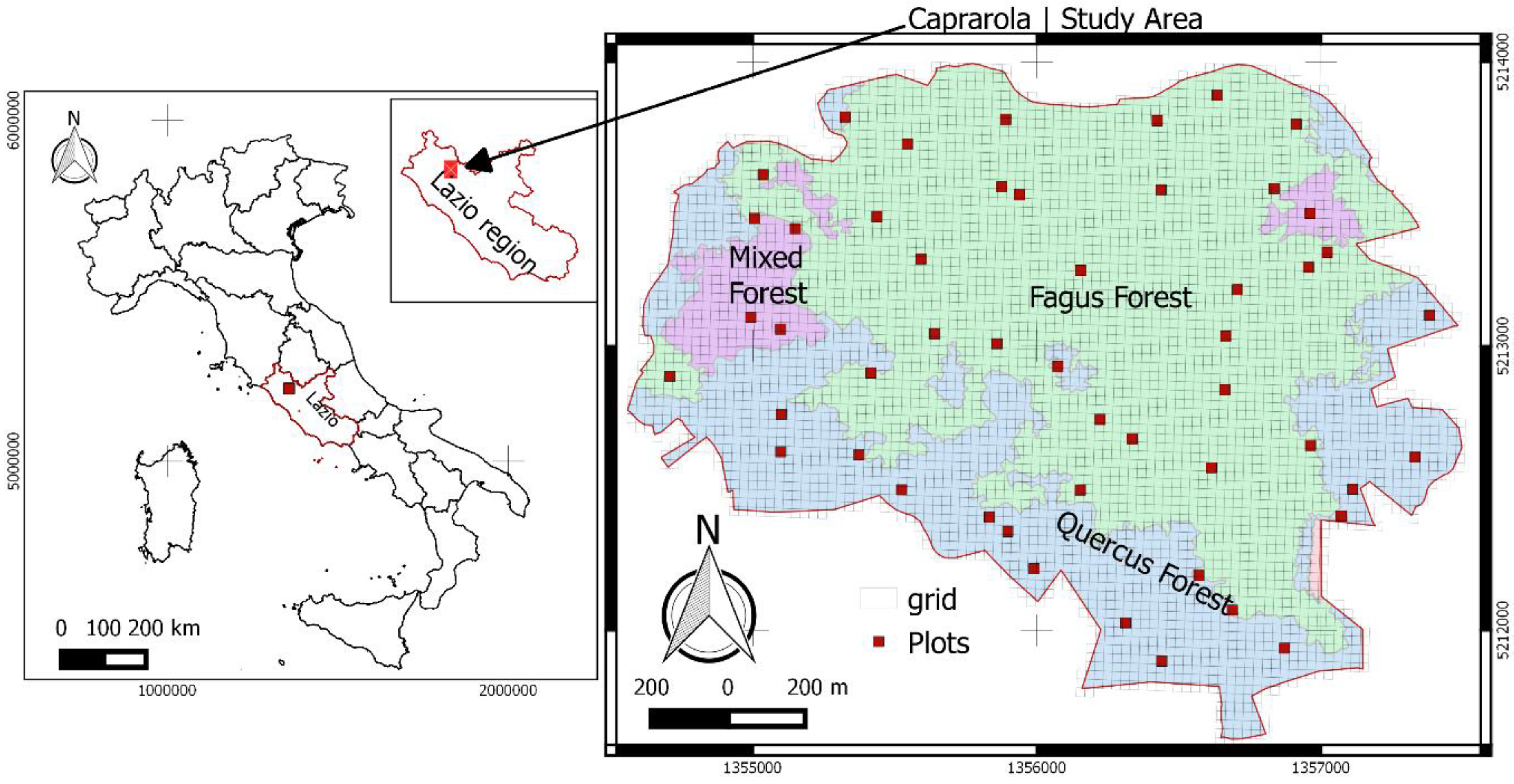
The test site extends over 240 hectares on the slopes of Mount Venere (500–800 m a.s.l.) in Caprarola Municipality (Central Italy). In the study, there were three forest types (Figure 1): beech-dominated forest (Fagus sylvatica, 149 ha), turkey oak forest (Quercus cerris, 76 ha), and mixed forest of the two species (14 ha). The vertical profile is, to a large extent, mono-layered in the beech forest and bi-layered in the other two forest types.

The presence of very fertile volcanic soils and the microclimate as a result of the presence of a lake create favorable conditions for the growth of beech, even at a low elevation. In fact, the conformation of the basin, the frequent formation of mists, the high relative air humidity, and the protection from extreme winds ensure a suitable habitat for this species. As a result, the beech forest of Monte Venere is ecologically important, as it grows at much lower altitudes (around 500 m above sea level) than those usually occupied by beech in the Central Apennines (optimum between 1000 and 1700 m a.s.l.).

Beech forest of Monte Venere belongs to the Aquifolio-Fagetum association, which reaches the extreme northern boundary of its ecological range in the Province of Viterbo [40]. Beech is usually accompanied by other deciduous trees like Quercus cerris L. (turkey oak) in the upper layer and only at lower altitudes, and by Carpinus betulus L. (hornbeam), Castanea sativa Mill. (Chestnut), Acer opalus L. (maple), Corylus avellana L. (hazel), and Ilex aquifolium L. (holly) in the dominated layer.

Turkey oak becomes the dominant species on the south-facing aspects. Turkey oak forests also contain accompanying species such as ash (Fraxinus ornus L.) and hornbeam (Ostrya carpinifolia L.). Turkey oak forests present a well-developed shrub layer including Rosa canina L., Cornus sanguinea L., Crataegus monogyna Jacq., Crataegus oxychanta L., and Ruscus aculeatus L.

The test site contains 50 forest inventory plots, each 23 m × 23 m in dimension (area of the plot 529 m²), distributed according to a one-per-stratum systematic sampling design. This sampling scheme partitions the study area into square grids of 529 m² plots spatially aggregated into 50 equal size strata. One sample-site location is independently and randomly selected in each stratum, resulting in the spatial distribution displayed in Figure 1. There were 28, 13, and 9 plots in beech, turkey oak, and mixed forests, respectively.

2.2. Field Data Processing

The spatial position of the center of inventory plots was recorded with a sub-meter accuracy Trimble GEO7X GNSS receiver and was post-processed with data from local base stations situated approximately 30 km from the study area. At each plot, all plants (trees and shrubs) with a diameter at breast height (DBH) greater than 2.5 cm were inventoried during the 2016 growing season. Key measurements included species identification, diameter at breast height (DBH), tree height, and the presence of microhabitat-bearing living trees according to the reference catalogue provided by Winter and Möller [41]. These elements, which are characteristic of natural forests, especially of the old-growth phases, are often absent or rare in managed forests and are, therefore, considered key indicators of biodiversity.

Tree and shrub data were processed in the present study to distinguish the understory species from canopy trees (living trees). The understory layer was identified as the layer including plants with heights up to 50% of the maximum tree height observed in the plot [42]. In each plot, we calculated for the understory:

(1) density and development, by means of the parameters such as number of plants (N_PLANTS), mean DBH (MEAN_DBH), mean plant height (MEAN_HTOT), total basal area (G_TOT), and total understory volume (V_TOT), which is calculated based on species-specific allometric equations developed using a combination of height and diameter;

(2) species diversity, by means of number of species (N_SPECIES), Shannon’s index (I_SHANNON, H’) [43], and Pielou index (I_PIELOU) [44].

Data collected on living trees were processed to derive structural data (mean DBH, MEAN_DBH; mean total height, MEAN_HTOT) and biodiversity data such as number of habitat trees (HAB), percentage of habitat trees (%HAB) of total number of plants in the plot, vertical species profile by the index of Pretzsch (I_PRETZSCH), Shannon’s index (I_SHANNON), and Margalef index (I_MARGALEF) [45].

Table 1. Summary of diversity indices.

Indices	Formulae	Range of Variation	Description
Shannon index ($H^{\prime }$)	$-{\displaystyle \sum }{p}_i\ln \left(p_i\right)$	[0,ln(S)]	The Shannon index expresses the frequency of the i-th species in a community; its values generally lie between 0 and 3.5; higher values correspond to higher species diversity. Its maximum value (MAX_SHANNON) is given by the natural logarithm of the number of species found in the test area and occurs when all species are equally present.
Pielou index ($E$)	$H^{\prime }/\ln \left(S\right)$	[0,1]	The Pielou index measures the relative abundance of species groups. The index can take values between 1 (all species are equally abundant) and 0 (there is only one species).
Pretzsch index ($A_p$)	$-{\displaystyle {\displaystyle \sum }_{i=1}^S}{\displaystyle {\displaystyle \sum }_{j=1}^Z}{p}_{ji}\ln \left(p_{ij}\right)$	[0,ln(SxZ)]	The Pretzsch index summarizes and quantifies species diversity and the vertical distribution of species in a forest. The index is lowest in one-story pure forests, whereas it rises for pure forests with two or more stories. Peak values are reached in mixed woodlands with heterogeneous structures.
Margalef index ($D$)	$\left(S-1\right)\ln \left(N\right)$	[0,∞)	It quantifies the presence of a number of species in a community. It also depends on the number of plants found in the sampling area. The index value increases with increasing species diversity.

S = number of species; N = total number of plants; pij = the frequency of species i in the layer j; pi = frequency of the specie i. z = number of layers.

displays the summary of biodiversity indices computed for each plot.

2.3. UAV Data

Aerial images of the study area were collected near peak greenness during two consecutive days of the last week of May 2016 by a fixed-wing eBee UAV (SenseFly, Cheseaux-Losanne, Switzerland). The eBee was equipped with a commercial SONY WX 18.MP RGB camera, recording in blue (450 nm), green (520 nm), and red (660 nm) wavelengths. The eBee, a hand-launched fixed-wing UAV with an electric motor-driven pusher propeller, has a 96 cm wingspan and a weight of about 700 g including camera, inertial measuring unit, GPS, and battery payloads. The maximum area covered in a single flight is about 140 ha at 120 m altitude or 9 km² at 2,000 m altitude, with a maximum flight time of 45 min.

Before UAV image acquisition, 15 ground control points (GCPs) were placed in open areas on the ground using 50 × 50 cm targets with a black and white chalkboard pattern to ensure high visibility in the images. The coordinates of the center of the GCPs were recorded with a Trimble Geo 7X receiver, with a 2-s logging rate for approximately 15 min each. The recorded coordinates were post-processed with data from the nearest ground station, located at 30 km from the study area, using the Pathfinder software. The post-processed GCP coordinates resulted in an average standard deviation from north and east and heights of 0.9 m, 0.7 m, and 1.9 m, respectively.

The flight altitude was 145 m above ground level, and the flight lines were set to obtain a longitudinal overlap of 85% and lateral of 75%. The total flight time was 2 h and 43 min among eight flights, launched from two different areas. Flight line spacing was 42 m, and the distance between two adjacent photos was 34.6 m. The focal length of the camera was set to 4 mm, and the ISO sensibility was ISO-100 with a shutter speed of 1/2000 s. A total of 433 images was acquired with a field of view of 200 m × 150 m.

Visual inspection of the acquired images revealed no problems related to light and atmospheric conditions or saturation. Orthomosaic images were derived from the UAV images using the SfM photogrammetry software Agisoft PhotoScan Pro [46]. This software allows one to fully automate the photogrammetric workflow to process aerial images and produce 3D (e.g., image-based point cloud) and 2D (e.g., Digital Surface Model and Ortomosaic) models, thanks to the multi-view stereo-matching and SfM algorithm implemented. This software has been already used for forest analysis [11,13,47,48,49,50], and the UAV images were processed using the following steps: (a) image alignment, (b) mesh building, (c) guided marker positioning and optimization of camera alignment (georeferencing of created scene), (d) dense cloud building, (e) raster grid DSM generation with a resolution of 0.2 m × 0.2 m, and (f) building orthomosaic. From the SfM photogrammetric workflow, we obtained a raster grid orthomosaic with a spatial resolution of 10 cm.

2.4. Methods

2.4.1. Image Processing and Variable Selection

We tested different settings of the Contrast Split segmentation algorithm to map forest canopy openings from the RGB orthomosaic images. The red band was the only one that significantly changed with openings in the canopy cover and the crowns. The Contrast split algorithm is considered effective in separating dark objects from bright objects [51]. The purpose of testing different settings was to extract forest canopy openings as accurately as possible, which are expected to appear darker, compared to surrounding canopy pixels. This process was accomplished using eCognition Developer (http://www.ecognition.com) software. We validated the gap delineation from contrast split segmentation by visual interpretation of the orthomosaic image to identify omission or commission errors. The visual validation techniques have been often used in forest canopy gap mapping [33]. We later tested different thresholds to filter small openings that might not affect ecological phenomena under investigation and, therefore, constitute a noise masking of relevant data. We only considered mapped features falling within the plot boundary and gaps within the plot boundary for at least 50% of their area. For each feature, we calculated the shape and size indices and other gap patch metrics commonly used in landscape-scale analyses. In total, 19 patch metrics (see Supplements; more details in [52]) were processed for each gap in each plot. This suite of metrics reflects different nuances of two- dimensional gap properties that may be potentially important for linking image-detected higher-level structures to dependent lower- level processes of the biota [37].

The size or extent gap patch metrics are the area (A), length, border length (or the perimeter), ratio of length/width, and the width. The shape metrics include border index (B.Index), asymmetry (Asym), roundness (Round), compactness (Comp), shape index, density, rectangular fit (Rect.fit), radius of the largest enclosed ellipse (RLE), radius of the smallest enclosed ellipse (RSE), elliptic fit, and other composite indices such as the shape complexity index (GSCI). The gap shape complexity index is an important measure of forest gaps [53]. It is the ratio of a gap’s perimeter to the perimeter of a circular gap of the same area. A value of 1 describes a perfect circle, while increasing values indicate increasing shape complexity. For example, values of 1.20 and 2.70 have 20% and 170% complexity, respectively. The last three gap metrics are the patch fractal dimension (PFD) [54], the fractal dimension (FD) [55], and the fractal dimension index (FDI) [56]. A description of each metric and its range of variation is given in

Table A1. Summary description of patch metrics.

Patch Metric	Formula	Values Range	Description
Border length ($b_v$)		[0, ∞)	Is basically the perimeter of the gap
Length ($l_v$)	$\sqrt{p_v\cdot {\gamma }_v}$	[0, ∞)	$p_v$ is the total number of pixels contained in the patch v ${\gamma }_v$ is the length-width ratio of an image object v
Length/Width (${\gamma }_v$)	-	[0, ∞)	The length-to-width ratio of an image object
Width ($w_v$)	$\frac{p_v}{{\gamma }_v}$	[0, ∞)	The width of an image object is calculated using the length-to-width ratio
Asymmetry	-	[0,1]	The Asymmetry feature describes the relative length of an image object, compared to a regular polygon. An ellipse is approximated around a given image object, which can be expressed by the ratio of the lengths of its minor and the major axes. The feature value increases with this asymmetry
Border Index	$\frac{b_v}{2\cdot (l_v+w_v)}$	[1, ∞) 1 = ideal	The Border Index feature describes how jagged an image object is; the more jagged, the higher its border index. This feature is similar to the Shape Index feature, but the Border Index feature uses a rectangular approximation instead of a square. The smallest rectangle enclosing the image object is created, and the border index is calculated as the ratio between the border lengths of the image object and the smallest enclosing rectangle
Compactness	-	[0, ∞) 1 = ideal	The Compactness feature describes how compact an image object is. It is similar to Border Index, but is based on area. However, the more compact an image object is, the smaller its border appears. The compactness of an image object is the product of the length and the width, divided by the number of pixels
Density	-	[0, depending on shape of image object]	The Density feature describes the distribution in space of the pixels of an image object. In eCognition Developer 9.0, the most “dense” shape is a square; the more an object is shaped like a filament, the lower its density. The density is calculated by the number of pixels forming the image object divided by its approximated radius, based on the covariance matrix
Elliptic Fit	-	[0,1]; 1 = complete fitting, 0 = <50% fit.	The Elliptic Fit feature describes how well an image object fits into an ellipse of similar size and proportions. While 0 indicates no fit, 1 indicates a perfect fit. The calculation is based on an ellipse with the same area as the selected image object. The proportions of the ellipse are equal to the length to the width of the image object. The area of the image object outside the ellipse is compared with the area inside the ellipse that is not filled by the image object
Radius of Largest Enclosed Ellipse (${\epsilon }_v^{\max }$)	-	[0, ∞)	The Radius of Largest Enclosed Ellipse feature describes how similar an image object is to an ellipse. The calculation uses an ellipse with the same area as the object and is based on the covariance matrix. This ellipse is scaled down until it is totally enclosed by the image object. The ratio of the radius of this largest enclosed ellipse to the radius of the original ellipse is returned as a feature value
Radius of Smallest Enclosing Ellipse (${\epsilon }_v^{\min }$)	-	[0, ∞)	The Radius of Smallest Enclosing Ellipse feature describes how much the shape of an image object is similar to an ellipse. The calculation is based on an ellipse with the same area as the image object and based on the covariance matrix. This ellipse is enlarged until it encloses the image object in total. The ratio of the radius of this smallest enclosing ellipse to the radius of the original ellipse is returned as a feature value
Rectangular Fit	-	[0,1] ; where 1 is a perfect rectangle.	The Rectangular Fit feature describes how well an image object fits into a rectangle of similar size and proportions. While 0 indicates no fit, 1 indicates for a complete fitting image object. The calculation is based on a rectangle with the same area as the image object. The proportions of the rectangle are equal to the proportions of the length to width of the image object. The area of the image object outside the rectangle is compared with the area inside the rectangle
Roundness	${\epsilon }_v^{\max }-{\epsilon }_v^{\min }$	[0, ∞); 0 = ideal	The Roundness feature describes how similar an image object is to an ellipse. It is calculated by the difference of the enclosing ellipse and the enclosed ellipse
Shape Index	$b_v/4\sqrt{A}$	[1,∞) ; 1 = ideal	The Shape index describes the smoothness of an image object border. The smoother the border of an image object is, the lower its shape index
Gap shape complexity index (GSCI)	$b_v/\sqrt{4\pi A}$	[1,∞) ; 1 = perfect circle	It is the ratio of a gap’s perimeter to the perimeter of a circular gap of the same area
Patch fractal dimension (PFD)	$2\cdot ln(b_v)/ln(A)$	-	-
Fractal dimension (FD)	$2\cdot ln(b_v/4)/ln(A)$	-	-
fractal dimension index (FDI)	$2\cdot ln(b_v/\sqrt{4\pi })/ln(A)$	-	-

(Appendix A).

For each patch metric, we calculated the median (mdn), mean (avg), standard-deviation (SD), sum (SUM), and the coefficient of variation (cv) per plot. We tested gap metrics with two different gap size thresholds, namely, greater than 1 m² and greater than 2 m². This leads to two times 95 variables for each plot. These two thresholds were set, because some ecological phenomena, such as understory structure dependencies, are only quantifiable if small gaps are taken into account, yet very small gaps may not affect at all the lower dependency phenomenon and therefore constitute noise [57].

2.4.2. Statistical Analysis

First, we performed exploratory analysis with the field data using ANOVA (Analysis of Variance) tests when the distribution was normal, and KRUSKAL-WALLIS analysis otherwise with the categorical variable being the forest type characterizing each single plot. Statistical analyses were performed with R Foundation 3.2.3 (https://www.r-project.org/foundation/). The code used in this paper is available at https://github.com/MartinBagaram/forest_gaps.

We used all gap variables for Pearson’s product-moment correlation analysis and Spearman’s rank correlation with the field data, using post-stratification of sampling units by forest types where appropriate. Usually, the two correlations give approximately the same results (see [58]). To avoid the fact that the observed correlation, although significant according to the p-value lower than 5%, could have occurred by chance, its significance was further tested using the 9999 permutation method proposed by Legendre and Legendre [59]. This method has been successfully used in investigating the relationship between forest canopy gap metrics and biodiversity [37].

For gap variables correlated with field data, we tested the correlation among significant potential predictors. This third step allowed a decrease in the redundant information brought by potentially correlated predictors and eliminated the collinearity or singularity. To determine the most significant variables to be used as possible predictors, we used a forward stepwise analysis, since this approach selects only the minimum significant number of predictors. There exist three methods for model selection known as best, forward, and backward subset selection. In general, the three methods lead to similar though not identical results [60]. Owing to the huge number of predictors (190 in this study), the best subset selection requires for each field parameter to compare up to two of 190 models, which deterred us from using the best set selection.

When the forward stepwise yielded only one predictor variable as sufficient to model the field parameter (which was often the case), we compared the correlation coefficients of Spearman and Pearson. If these two coefficients were significant and close to one another, then the patch metric was selected as a predictor if it passed the 9999 permutations test of Legendre. Otherwise, the second variable with the highest values of both Spearman and Pearson coefficients was selected, and then we repeated the 9999 permutations method. This approach has the advantage of, on one hand, excluding variables depicting high Pearson’s correlation due to extreme values, and on the other hand, not solely relying on the Spearman’s correlation, which is a measure of monotony [61] and not of linearity. Furthermore, using 9999 permutation assures that the p-value observed does not occur by chance.

Finally, we performed linear regression tests using the selected significant variables. Following Møller and Jennions [62] and Getzin et al. [37], who considered a coefficient of determination R² > 0.25 as meaningful, since the predictor value leads to a great change if it explains over 25% of variance, we used a threshold of R² > 0.5. We then validated the regression by checking regression quality assumptions such as the normality of residuals, the homoscedasticity of residuals, and that the mean of the residuals is zero. For forest parameters that can be predicted with R² greater than 50%, we generalized the model to the whole forest type extent using the grid of 529 m² plots. We performed the validation with cross-validation (Leave-One-Out Cross-Validation), which produced root mean squared errors (RMSE).

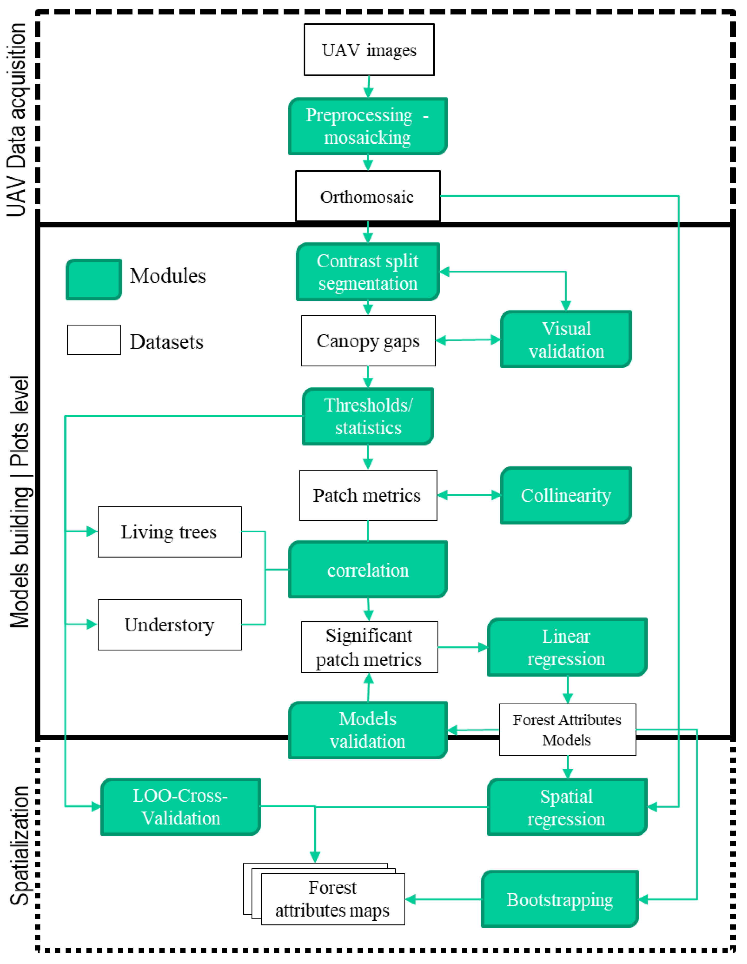
For inference, it is important to provide the variance, confidence interval, and bias of R². Bootstrapping is a method commonly used for that purpose [63,64,65], especially in the case of linear regression [66]. Bootstrap is a resampling method developed by Efron and Tibshirani [67]. We computed those statistics for variables with R² greater 0.50 using formulas given by Mura et al. [63]. Although it is suggested that the bootstrap sample size should be big enough (greater than 200), there is no consensus yet on what should be the actual size. Following Mura et al. [63], we set the bootstrap sample size to 500. The mapping of biodiversity attributes was achieved with ArcGIS 10.2. A graphical abstract of the methodology is presented in Figure 2.

3. Results

3.1. Canopy Gaps Mapping

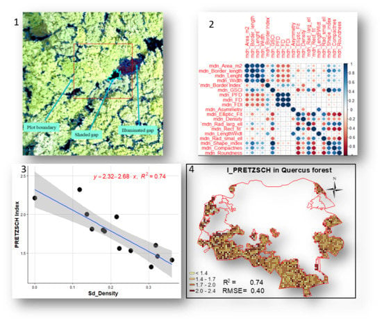
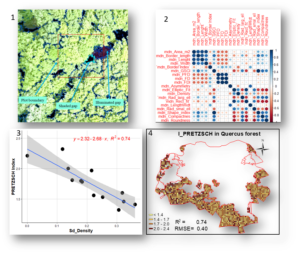
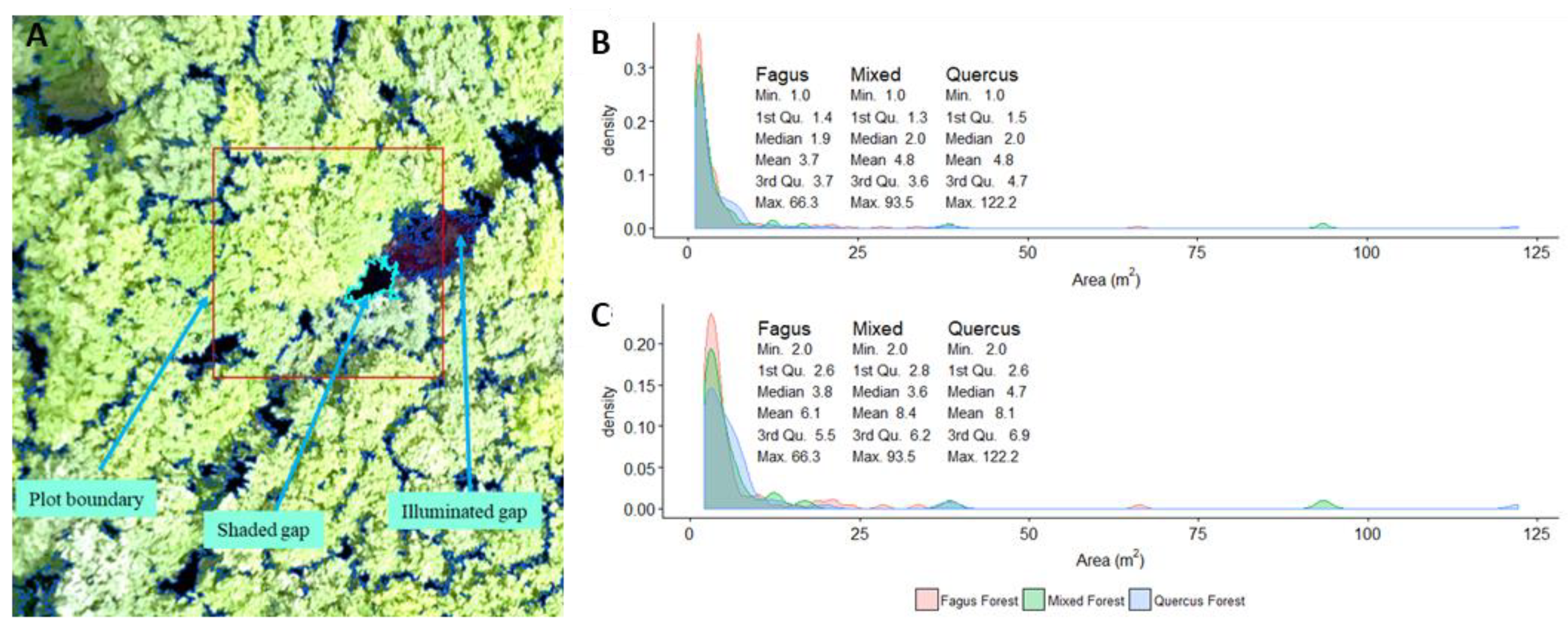
The contrast split algorithm based on the red band accurately differentiated dark objects (shaded canopy gaps) from bright objects, which, in most cases, corresponded to forest canopy. The mapping faithfully delineated shaded canopy gaps but performed poorly in illuminated gaps when the bare soil was apparent (Figure 3). Detected gaps from plots ranged from 100 cm² (1 pixel) to 122 m². This range encompassed small openings or inter-crown cracks in the canopy cover and larger gaps generated by the fall of one or more canopy trees. The gap size distribution is roughly the same in the three forest types. When considering gaps greater than 1 m², over 75% of gaps in the three forest types were less than 5 m². When considering gaps greater than 2 m², over 75% of gaps in the three forest types were less than 7 m² (Figure 3).

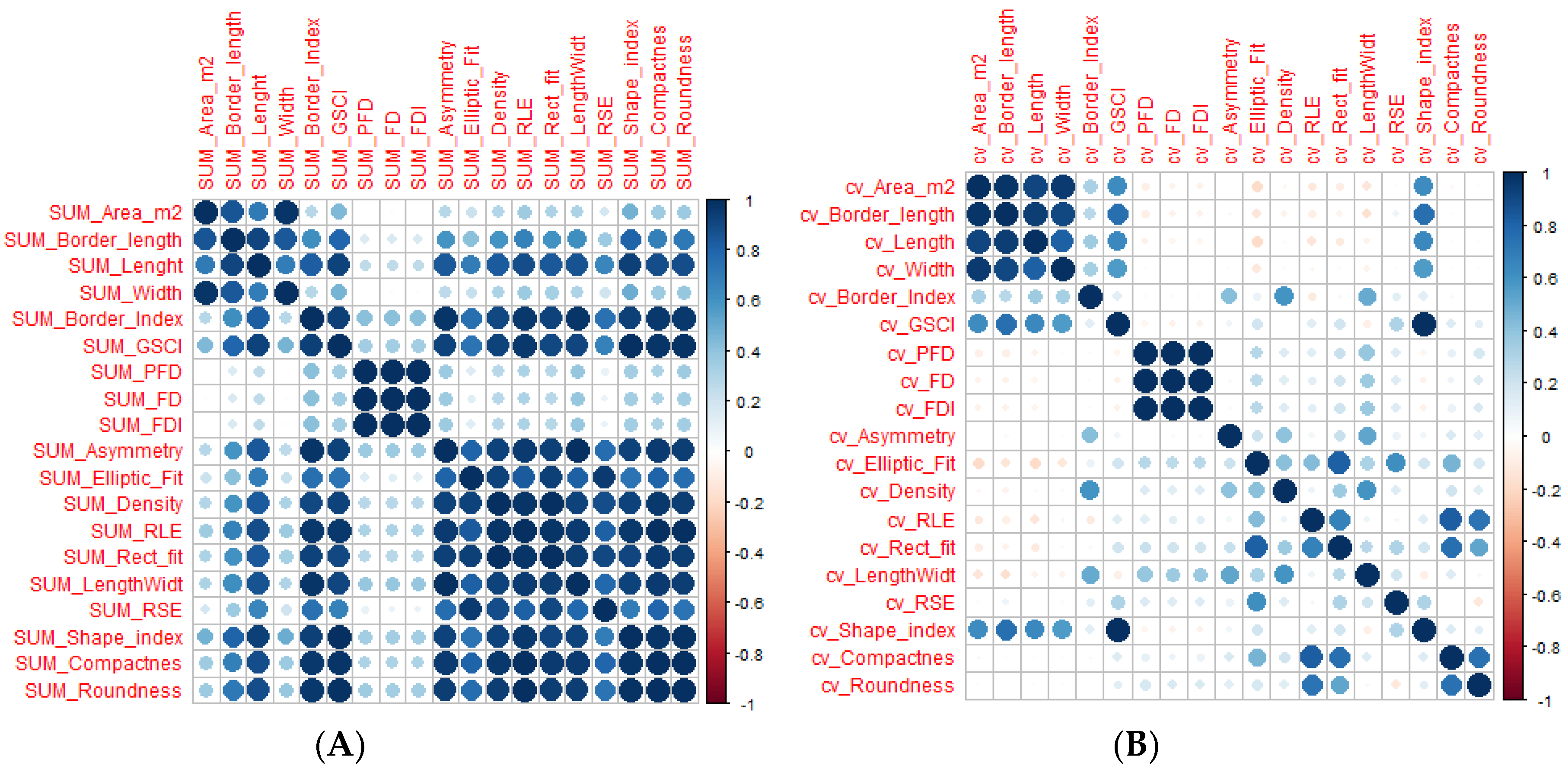
The collinearity analysis of gap patch metrics indicated that patch metrics were strongly correlated to each other. A sample result of collinearity analysis of predictor variables is reported in Figure 4. The lowest correlations were obtained with the coefficient of variation, whereas the highest correlations were associated with the plot-level sum of patch metrics. These findings indicate that gap patch metrics are not suitable for a multiple linear regression.

3.2. Correlation between Gap Metrics and Understory Variables

The understory layer exhibits density, development, and diversity features that seem to vary with forest types cover. Namely, variables related to density, development, and diversity of the understory had significant differences amongst the forest types, except for Pielou index, MEAN_HTOT, and MEAN_DBH (

Table 2. Summary of exploratory statistics on understory data.

Normal Distributed Variables
Variables	ANOVA	TUKEY
Pielou index (I_PIELOU)	no significant difference
Mean total height (MEAN_HTOT)	no significant difference
Variables Non Normal
Variables	KRUSKAL-WALLIS	MANN-WHITNEY
Number of plants (N_PLANTS)	***	(1 vs. 2) ***; (2 vs. 3) **
Number of species (N_SPECIES)	***	(1 vs. 2) ***; (1 vs. 3) **
Shannon index (I_SHANNON)	***	(1 vs. 2) ***; (1 vs. 3) **
Mean DBH (MEAN_DBH)	no significant difference
Total basal area (G_TOT)	***	(1 vs. 2) ***
Total volume (V_TOT)	**	(1 vs. 2) **

* p < 0.05; ** p < 0.01; *** p < 0.001; 1 = beech forest; 2 = oak forest; 3 = mixed forest.

).

All eight field parameters presented significant correlations (p < 0.05), with gap patch metrics in at least one of the three forest types (

Table 3. Results of linear regression with understory data (B = slope of linear regression; SE = standard error, N = sample size). Bold values refer to adjusted R² higher than 50%.

Quercus Forest

N_PLANTS

N_SPECIES

I_SHANNON

I_PIELOU

N = 13

B

SE (B)

R2

p-value

B

SE (B)

R2

p-value

B

SE (B)

R2

p-value

B

SE (B)

R2

p-value

Linear regr.

Linear regr.

Linear regr

Linear regr

Intercept

−28.85

16.8

Intercept

7.21

0.71

0.000

Intercept

1.70

0.13

0.000

Intercept

1.02

0.10

0.000

Mdn_GSCI

18.61

5.24

0.49

0.005

Sd_rect.fit

−20.66

7.02

0.39

0.013

Sd_rect.fit

−4.83

1.28

0.52

0.003

Sd_Density

−1.10

0.41

0.34

0.021

MEAN_DBH

MEAN_HTOT

V_TOT

G_TOT

N = 13

B

SE (B)

R2

p-value

B

SE (B)

R2

p-value

B

SE (B)

R2

p-value

B

SE (B)

R2

p-value

Linear regr.

Linear regr

Linear regr

Linear regr

Intercept

−23.27

7.38

0.009

Intercept

9.54

1.04

Intercept

5.34

1.48

0.004

Intercept

1.05

0.35

0.012

Avg_rect.fit

48.39

11.43

0.60

0.001

Mdn_B.Index

−56.61

24.15

0.27

0.039

Mdn_Asym.

−6.60

2.36

0.36

0.018

Avg_Asym

−1.36

0.59

0.26

0.041

Mixed forest

N_PLANTS

N_SPECIES

I_SHANNON

I_PIELOU

N = 9

B

SE (B)

R2

p-value

B

SE (B)

R2

p-value

B

SE (B)

R2

p-value

B

SE (B)

R2

p-value

Linear regr.

Linear regr

Linear regr

Linear regr

Intercept

47.02

9.62

0.002

Intercept

0.86

0.93

Intercept

0.11

0.35

Intercept

0.1

0.3

Avg_Round.

−23.79

6.40

0.62

0.007

Mdn_RSE

8.29

2.92

0.47

0.025

Mdn_RSE

2.73

1.08

0.40

0.040

Avg_RLE

0.42

0.17

0.43

0.045

MEAN_DBH

MEAN_HTOT

G_TOT

V_TOT

N = 9

B

SE (B)

R2

p-value

B

SE (B)

R2

p-value

B

SE (B)

R2

p-value

B

SE (B)

R2

p-value

Linear regr.

Linear regr

Linear regr

Linear regr.

Intercept

9.70

0.82

0.000

Intercept

0.90

0.82

Intercept

−0.02

0.05

Intercept

3.48

1.23

0.026

Sum_width

−0.00

0.00

0.51

0.018

avg_Asym

10.39

1.40

0.87

0.000

Sd_Asym.

0.59

0.21

0.45

0.027

Avg_Comp

−1.16

0.48

0.37

0.048

Fagus forest

N_SPEIES

I_SHANNON

I_PIELOU

MEAN_HTOT

N = 28

B

SE (B)

R2

p-value

B

SE (B)

R2

p-value

B

SE (B)

R2

p-value

B

SE (B)

R2

p-value

Linear regr.

Linear regr

Linear regr

Linear regr

Intercept

3.13

0.77

0.000

Intercept

1.01

0.29

0.002

Intercept

0.26

0.18

Intercept

5.46

1.40

0.000

Cv_Round.

−6.02

2.64

0.15

0.033

Sd_Round.

−1.85

0.72

0.21

0.018

Mdn_PFD.

0.06

0.02

0.48

0.022

Cv_Length

11.14

4.20

0.23

0.016

).

Table B1. Coefficient of correlations of Pearson and Spearman for some selected explicative and understory dependent variables in Quercus forest.

	N_PLANTS	N_SPECIES	I_SHANNON	I_PIELOU	MEAN_DBH	MEAN_HTOT	V_TOT	G_TOT
	Mdn_GSCI	Sd_Rect.fit	Sd_Rect.fit	Sd_Density	Avg_Rect.fit	Mdn_B. Index	Mdn_Asy	Avg_Asy
Threshold	1 m2	2 m2	2 m2	1 m2	1 m2	2 m2	1 m2	1 m2
Pearson	0.73	−0.66	−0.75	−0.64	0.79	−0.58	−0.64	−0.57
Spearman	0.70	−0.73	−0.88	−0.68	0.75	−0.67	−0.57	−0.55

,

Table B2. Coefficient of correlation of Pearson and Spearman for some selected explicative and dependent variables in mixed forest.

	N_PLANTS	N_SPECIES	I_SHANNON	I_PIELOU	MEAN_DBH	MEAN_HTOT	G_TOT	V_TOT
	Avg_Round.	Mdn_RSE	Mdn_RSE	Avg_RLE	Sum_width	Avg_Asym.	Sd_Asym.	Avg_Comp.
Threshold	2 m2	1 m2	1 m2	2 m2	2 m2	2 m2	2 m2	2 m2
Pearson	−0.81	0.73	0.69	0.71	−0.78	0.94	0.72	−0.67
Spearman	−0.83	0.70	0.70	0.75	−0.70	0.92	0.72	−0.77

and

Table B3. Coefficient of correlation of Pearson and Spearman for some selected explicative and dependent variables in Fagus forest.

	N_SPECIES	I_SHANNON	I_PIELOU	MEAN_HTOT
	Cv_Round	Sd_Round	Mdn_PFD	Cv_Lenght
Threshold	1 m2	1 m2	1 m2	2 m2
Pearson	−0.43	0.50	0.74	0.52
Spearman	−0.45	0.56	0.87	0.57

of Appendix B present the threshold, Pearson’s, and Spearman’s correlations of gap patch metrics and understory. The regression coefficient had the lowest standard error in mixed and Fagus forests compared to Quercus forest; MEAN_DBH in mixed forest had a very low variability as shown by the coefficient of the regression predicting MEAN_DBH in mixed forest is merely equal to zero.

As shown in Table 3, the highest coefficient of determination was in mixed forest (MEAN_HTOT, R² = 0.87, p < 0.000) and the lowest was in Fagus forest (N_SPECIES, R² = 0.15, p < 0.05). The best results were found in Quercus and mixed forests, whereas the worst ones were in Fagus forest. I_SHANNON and MEAN_DBH in Quercus forest, and MEAN_HTOT and N_PLANTS in mixed forest were predicted with R² > 0.50. All patch metrics, except one (cv_Length in Fagus forest), correlated with the field parameters were related to gap shape.

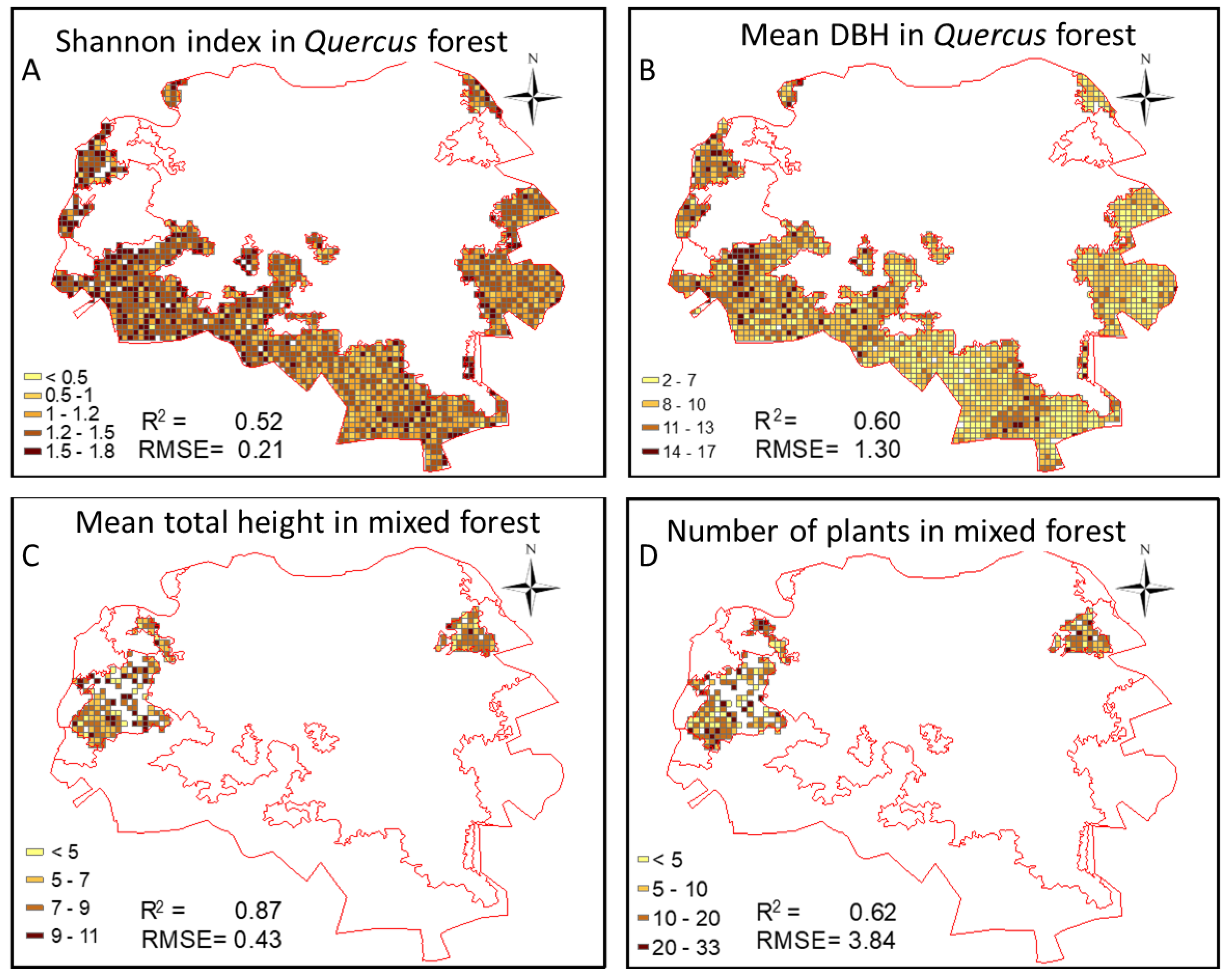
The spatial patterns of the understory models to the extent of their respective forest types underscored some key features (Figure 5). In Quercus forest, I_SHANNON ranged from just above 0 to 1.8 with RMSE of 0.21. These values are in the range of variation of data collected on plots. The variability in MEAN_DBH in Quercus forest was from 2 to 17 cm with an RMSE = 1.3 cm.

In mixed forest, MEAN_HTOT went up to 11 m, with the majority of grids falling between 5 and 9 m, and the RMSE was 0.43. The number of plants per grid ranged from less than 5 to 33 with an RMSE of 3.84 (Figure 5). We did not perform the spatialization of MEAN_DBH in mixed forest, even though the R² was greater than 0.5, because the linear model slope was close to zero. The empty cells in the figure correspond to cells in which the prediction gives unreasonable values.

3.3. Correlations between Gap Metrics and Living Tree Variables

All living tree diversity and structural variables exhibited significant differences among the three forest types, except total basal area (G_TOT) and total volume (V_TOT) (

Table 4. Summary of exploratory statistics on living trees.

Variables with Normal Distribution
Variables	ANOVA	TUKEY
Number of plants (N_PLANTS)	***	(1 vs. 2) ***; (2 vs. 3) ***
Pretzsch index (I_PRETZSCH)	***	(1 vs. 2) ***; (1 vs. 3) ***
Total basal area (G_TOT)	no significant difference
Total volume (V_TOT)	no significant difference
Number of habitat trees (HAB)	*	(1 vs. 2) **
Percentage of habitat trees (%_HAB)	**	(1 vs. 2)*
Non Normal Distributed Variables
Variables	KRUSKAL-WALLIS	MANN-WHITNEY
Number of species (N_SPECIES)	***	(1 vs. 2) ***; (1 vs. 3) ***
Margalef index (I_MARGALEF)	***	(1 vs. 2) ***; (1 vs. 3) ***
Shannon index (I_SHANNON)	***	(1 vs. 2) ***; (1 vs. 3) ***
Mean diameter at breast height (MEAN_DBH)	***	(1 vs. 2) ***; (2 vs. 3) ***
Mean total height (MEAN_HTOT)	**	(1 vs. 2)**

* p < 0.05; ** p < 0.01; *** p < 0.001; 1 = beech forest; 2 = oak forest; 3 = mixed forest.

). As with the understory, some gap patch metrics appear to be significantly correlated with these field parameters (p < 0.05).

Table C1. Coefficient of correlations of Pearson and Spearman for some selected explicative and living trees dependent variables in Quercus forest.

	N_SPECIES	I_SHANNON	I_MARGALEF	I_PRETZSCH	MEAN_DBH	MEAN_HTOT	HAB	%HAB
	Sd_rect_fit	Cv_Density	Sd_rect_fit	Sd_Density	Sum_Rect.fit	Mdn_Rect.fit	Sum_Rect.fit	Sum_RLE
Threshold	2 m2	2 m2	2 m2	2 m2	1 m2	1 m2	2 m2	2 m2
Pearson	−0.68	−0.64	−0.71	−0.87	0.61	0.59	−0.79	−0.71
Spearman	−0.72	−0.61	−0.74	−0.90	0.70	0.56	−0.70	−0.64

,

Table C2. Coefficient of correlations of Pearson and Spearman for some selected explicative and living trees dependent variables in mixed forest.

	MEAN_DBH	MEAN_HTOT	HAB	%HAB
	Avg_Round.	Sd_Asym.	Cv_Length	Avg_RSE
Threshold	2 m2	1 m2	2 m2	1 m2
Pearson	0.74	−0.84	−0.90	−0.83
Spearman	0.82	−0.95	−0.92	−0.92

and

Table C3. Coefficient of correlations of Pearson and Spearman for some selected explicative and living trees dependent variables in Fagus forest.

2m	HAB	%HAB
	Cv_PFD	Avg_RSE
Pearson	0.43	−0.38
Spearman	0.50	−0.39

in Appendix C summarize the threshold, Spearman’s, and Pearson’s correlations associated with gap patch metrics and living trees parameters. In Quercus forest, eight field parameters yielded good results, compared to mixed forest which had four. For Fagus forest, habitat trees and percentage of habitat trees only denoted significant correlations. Coefficients of the linear regression had the lowest standard errors in Quercus forest.

The highest coefficient of determination was in mixed forest (HAB, R² = 0.79, p < 0.000) and the lowest was in Fagus forest (%HAB, R² = 0.11, p < 0.05). Best results were in Quercus forest (I_PRETZSCH, HAB, and %HAB) and mixed forest (HAB, %HAB, MEAN_DBH, and MEAN_HTOT). HAB, %HAB, MEAN_HTOT in mixed forest and HAB and I_PRETZSCH in Quercus forest had R² exceeding 0.50 (

Table 5. Results of linear regression of living trees (B = coefficient of linear regression, SE = standard error, N = sample size). Bold values refer to adjusted R² higher than 50%.

Quercus forest

N_SPECIES

I_SHANNON

I_MARGLEF

I _ PRETZSCH

N = 13

B

SE (B)

R2

p-value

B

SE (B)

R2

p-value

B

SE (B)

R2

p-value

B

SE (B)

R2

p-value

Linear regr.

Linear regr

Linear regr

Linear regr

Intercept

8.13

0.71

0.000

Intercept

1.81

0.14

0.000

Intercept

1.94

0.18

0.000

Intercept

2.32

0.1

0.000

Sd_Rect.fit

−21.46

7.04

0.41

0.011

Cv_Density

−2.61

0.95

0.35

0.019

Sd_Rect.fit

−6.02

1.80

0.46

0.006

Sd_Density

−2.68

0.45

0.74

0.000

MEAN_DBH

MEAN_HTOT

HAB

%HAB

N = 13

B

SE (B)

R2

p-value

B

SE (B)

R2

p-value

B

SE (B)

R2

p-value

B

SE (B)

R2

p-value

Linear regr.

Linear regr

Linear regr

Linear regr

Intercept

11.30

3.42

0.007

Intercept

−15.73

11.99

Intercept

20.54

2.44

0.000

Intercept

41.87

5.45

0.000

Sum_rect.fit

1.29

0.50

0.32

0.02

Mdn_rect.fit

45.41

18.68

0.29

0.033

Sum_rect.fit

−3.10

0.73

0.59

0.001

Sum_RLE

−1.86

0.54

0.47

0.006

Mixed forest

MEAN_DBH

MEAN_HTOT

HAB

%HAB

N = 9

B

SE (B)

R2

p-value

B

SE (B)

R2

p-value

B

SE (B)

R2

p-value

B

SE (B)

R2

p-value

Linear regr.

Linear regr

Linear regr

Linear regr

Intercept

−10.86

13.32

Intercept

27.74

2.70

0.000

Intercept

14.34

1.20

0.000

Intercept

108.24

17.54

0.000

Avg_Round

25.92

8.86

0.49

0.022

Sd_Asym.

−49.06

11.72

0.67

0.004

Cv_Length

−14.01

2.51

0.79

0.000

Avg_RSE

−208.99

53.19

0.64

0.005

Fagus forest

HAB

%HAB

N = 28

B

SE (B)

R2

p-value

B

SE (B)

R2

p-value

Linear regr.

Linear regr

Intercept

4.00

1.21

0.003

Intercept

61.35

7.88

0.000

cv_PFD

11.82

5.23

0.15

0.034

Avg_RSE

−58.21

27.71

0.11

0.045

). Among the patch metrics correlated with living tree parameters, all but the length (cv_Length in mixed forest), which is gap size related patch metric, were gap shape-related patch metrics.

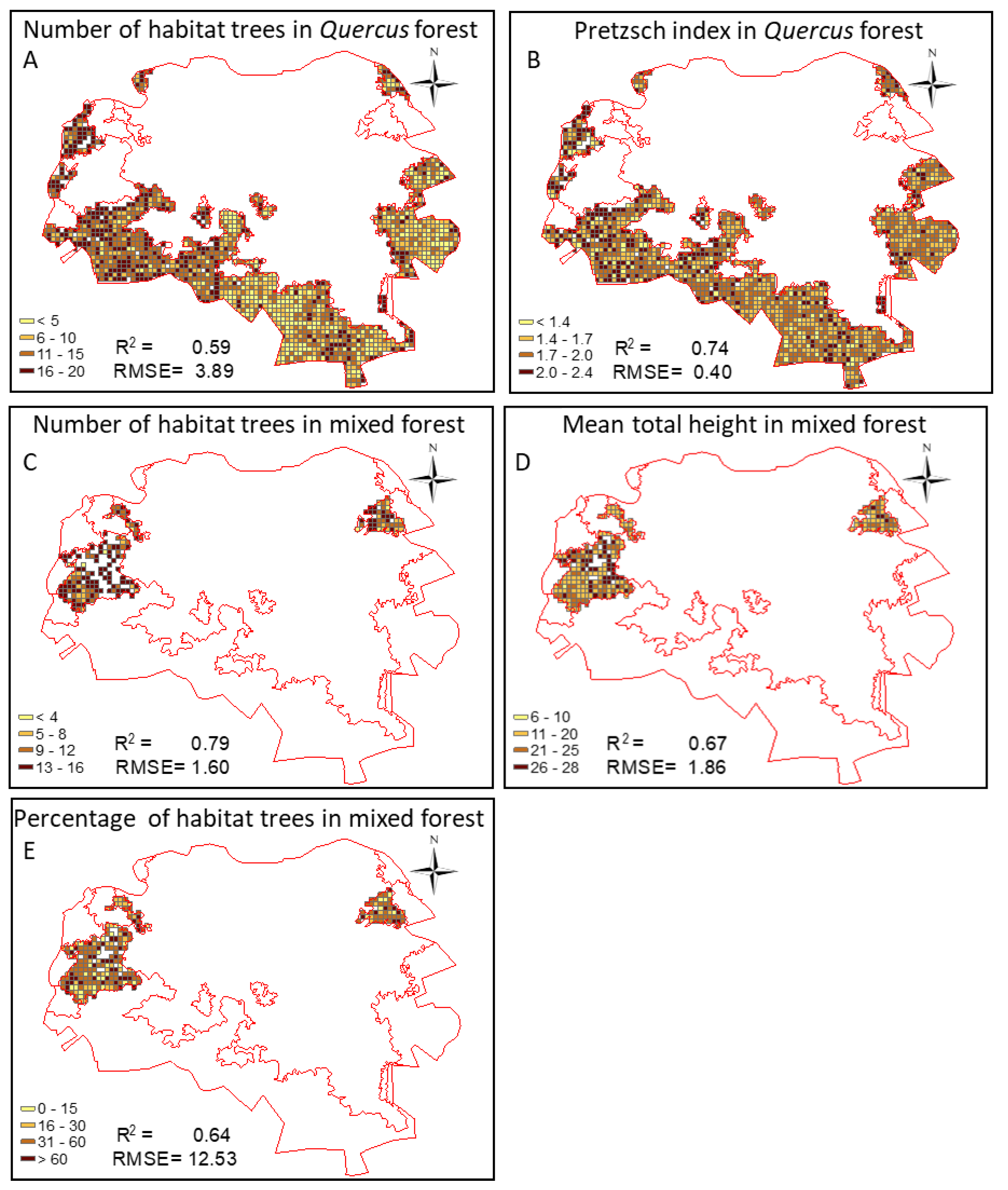
The spatial patterns of regression models for living trees parameters are presented in Figure 6. In Quercus forest, I_PRETZSCH varied from 1 to 2.4 with RMSE of 0.40. A majority of cell grids had indexes higher than 1.7, indicating a complex vertical structure. In the same forest type, the number of habitat trees reached 20 with RMSE of 3.89.

In mixed forest, however, most of cell grids had the number of habitat trees higher than 9. In this forest, the prediction error is relatively smaller with an RMSE of 1.6. The percentage of habitat trees per grid is more variable with values ranging from 0 to 100%. The MEAN_HTOT varied from 6 to 28 m with an RMSE of 1.86.

3.4. Quality Assessment

The bootstrap R² was relatively close to the experimental R² (computed from the actual data) for both the understory and the living trees. The standard error and the bias are very low. The highest negative bias was related to I_SHANNON with a bias of −0.05. This suggests that the actual R² of I_SHANNON is lower than the one observed. Similarly, the highest positive bias was recorded with HAB in mixed forest (living trees with a value of 0.03)suggesting that the actual R² associated with habitat trees in mixed forest is higher than 0.79 (

Table 6. Results of bootstrapping for parameters with R² greater than 0.50.

	Forest Types	Parameters	Bootstrap R2	Standard Error (95%)	R2	Bias
Understory	mixed	Mean total height	0.877	0.006	0.872	−0.005
		Number of plants	0.623	0.016	0.616	−0.007
		Mean DBH	0.507	0.022	0.515	0.008
	Quercus	Mean DBH	0.577	0.017	0.600	0.024
		Shannon index	0.576	0.010	0.523	−0.053
Living trees	Quercus	Pretzsch index	0.755	0.008	0.738	−0.016
		Number of habitat trees	0.554	0.018	0.586	0.032
	mixed	Mean total height	0.682	0.012	0.674	−0.008
		Number of habitat trees	0.757	0.014	0.790	0.032
		Percentage of habitat trees	0.627	0.019	0.644	0.017

).

4. Discussion

4.1. Mapping Forest Canopy Gaps

Gap mapping from UAV RGB 10 cm orthomosaic images produced very promising results. In this study, we mapped openings in canopy as small as 100 cm², corresponding either to intra-crown openings or to inter-crown cracks in the canopy cover. This fine-scale mapping of canopy openings is important, because some ecological phenomena, such as understory structure dependencies, are only quantifiable if small gaps are taken into account. Though it is known that different forests, depending on ecological and geographical contexts, exhibit different canopy structure, there is not yet a rule for a minimum gap size. As a consequence, different authors set, arguably, minimum gap size of 1 m² [8,37,57,68,69,70], 5 m² [71], 10 m² [33,72], and 50 m² [36]. To circumvent this problem, we did not set any gap size limit but let the ecological phenomenon under investigation dictate the appropriate gap size limit. Hobi et al. [73] used the same approach by not setting any gap size limit. The gap mapping used in this paper does not take into account the vegetation height. Therefore, our mapping, although consistent with the definition given by Brokaw [74], focuses only on shaded gaps or dark objects. Zielewska-Büttner et al. [33] reported as well that in their attempt to map forest canopy gaps, the shadow occurrence and forest height affected the mapping accuracy.

Other authors who mapped forest gaps from remote sensing used either LiDAR-derived forest canopy height models [53,68,70,75,76,77] or RGB imagery and photogrammetrically-derived canopy height model (CHM) [33,34,75,78]. Alternatively, fish eye [79] airborne lidar derived data [76,80] or terrestrial laser scanning [81] can be used. All those techniques, although effective, are not affordable for small forest land owners.

Furthermore, the forest canopy mapping was highly affected by the quality of the orthomosaic and image acquisition conditions. In this study, the orthomosaic co-registration presented some flaws in certain areas. Those areas displayed a low quality in gap delineation and even in the visual interpretation of what constitutes a gap. The second limitation came from the difference in reflectance between the datasets acquired in the two consecutive days. Although the images were acquired at noon to reduce the bidirectional reflectance effect [22], the sun illumination between the two days was not the same, leading to two sets of images with slightly different brightness. The best practice would be to collect data covering the site in the same light conditions and, if possible, in the same day.

Finally, the contrast split algorithm failed to detect illuminated canopy gaps where the bare soil is visible, because the bare soil reflectance is as high as the one of the vegetation. Therefore, the algorithm missed big gaps with no vegetation but with apparent bare soil. As an alternative, multiresolution segmentation would allow one to detect both types of canopy gaps, though it requires all image objects to be subsequently classified by the user (more time consuming than contrast split). The second alternative would be to use image-based 3D point clouds. This dataset, possessing a third dimension, is sufficient for detecting local minima in the digital crown model, e.g., by means of hotspot analysis [82].

4.2. Modeling Understory Variables through Canopy Gaps Covariates

The very high-resolution mapping of gaps in the canopy cover provided a set of metrics that proved to be useful as covariates in regression estimation of the density (number of plants), the diversity (Shannon index) and the development (mean DBH, mean HTOT) of the understory in Quercus and mixed forest types. The same cannot be said for Fagus forest. One explanation for Fagus’ poorer performance lies in the different light conditions under Quercus and Fagus canopy cover. The crown of Turkey oak, when grown in fully stocked high forest, is oval-shaped, with high canopy base height and medium-textured. Due to this structure, oak does not cast a dense shadow, and therefore allows other trees or shrubs to grow in lower layer. By contrast, beech casts a dense shadow under which relatively few plants can grow (e.g., shade-tolerant seedlings of beech). As a result, the presence of relatively small openings in the canopy cover, as those mapped here (75% smaller than 7 m²), might have an influence on the growth and diversification of the understory in Quercus and mixed forest types. The same level of canopy openness is not sufficient to modify light availability under beech canopy cover. This is confirmed by the relatively low-density values of beech understory.

The patch metrics correlated to the understory parameters, in mixed and Quercus forest types, are all shape metrics (except for the mean DBH in mixed forest). The density and development of the understory in mixed forest tend to increase as gap shape fits to an ellipse. A similar trend is observed in Quercus forest, where the mean DBH positively correlates with gap shape, when it fits to a rectangular geometry. On the other hand, the negative correlation between the diversity of the understory in Quercus forest and its covariate (standard deviation of Rectangular fit) does not have a straightforward ecological interpretation.

It seems reasonable that the diversity and development of the understory can be affected by the micro-porosity pattern of canopy cover, which light can shine through. The cumulative effect of differently shaped small gaps affects understory development under forest canopies dominated by Turkey oak and mixtures between Turkey oak and beech. In fact, two different gaps with the same extent can have different shape metrics. Our findings suggest that regular shapes (rectangular or elliptic) are influential for understory density and diameter growth.

This is a relatively new finding, as most previous studies focused on relationships between gap size and understory features. Popma and Bongers [83], for instance, demonstrated that the growth and morphology of seedlings in a tropical rain forest depended on the size of gaps; likewise, the dominance of understory vegetation by shade tolerant species or shade intolerant species [84].

4.3. Modeling Living Trees Biodiversity through Canopy Gaps Covariates

As for the understory, strong correlations were found between canopy shape gap metrics and density of micro-habitat bearing living trees and vertical species profile in Quercus and mixed forest types. The patch metric correlated with the density of micro-habitat bearing trees in canopies dominated by Turkey oak are negatively related to the presence of gaps fitting into a rectangular shape (Sum_rect fit), whereas vertical diversification in species profile is negatively correlated with the variability of gap density (Sd_Density). This reflects variability from filament shape (low value) to high dense shape (square). In mixed forest stands, the density of micro-habitat bearing trees is negatively correlated to the variability of gap length (CV_Length), while the mean height of the stand is positively correlated with the variability in gap shape asymmetry (Sd_Asym).

There might be different interpretations for these findings. Firstly, one could assume that the presence of canopy openings affects the growth in diameter and height of living trees. Schliemann and Bockheim [72] stipulated that after the opening of the canopy, the increased solar radiation allows plants to grow faster. Accordingly, the observed micro-porosity of canopy cover might favor sunlight penetration into the canopy layer(s), enabling conditions for species distribution along the vertical profile. In addition, the increased exposure to weather conditions and biotic agents might influence micro-habitat differentiation along the trunk and branches (e.g., cavities and holes, injuries and wounds, trunk and crown breakage, epixilic species colonization). This idea was primarily developed by Runkle [85] who contended that, in a tree fall gap, the microclimate changes associated with the gap formation extend to the bases of trees surrounding the canopy gap. Secondly, one might argue that micro-habitat bearing trees, which are frequently old large trees, create a structural diversity in the forest canopy because of their multiple dead tops, bole, and top decays. This specific structure influences the canopy arrangement and, therefore, creates small canopy gaps with specific patch metrics that can be used as a footprint of habitat trees occurrence.

4.4. Comparison with Other Studies and Implications

In the Mediterranean region characterized by complex environmental conditions and high seasonal variability of vegetation properties, UAV remote sensing offers advantages for capturing canopy parameters correlated with biodiversity metrics, in terms of costs and precision compared to alternative remote sensing technologies. A potential niche UAV fills—by providing covariates combined with field-based forest inventory data—can be used in regression models for spatially-explicit estimation of forest biodiversity variables over small forest areas. This study showed that canopy openness metrics can be used to predict, by linear regression in certain types of broadleaved deciduous forests, understory features (density, development, and diversity), vertical species profile, and functional forest ecosystem attributes such as density of micro-habitat bearing trees, which are considered difficult to measure directly [86]. This latter result is particularly interesting considering the recent attention given to the inventory of tree microhabitats [87].

The results obtained in this study are far from being random or happening by chance. The correlation was controlled using permutation tests [59], and all linear regression models satisfied linear regression assumptions. The confidence of the results was further bolstered by bootstrap resampling technique. To the best of our knowledge, this study is the first investigating the relationship between living tree parameters such as habitat trees and gap patch metrics from UAV RGB images.

Gap size distribution was roughly the same in the three forest types, with over 75% of gaps being smaller than 7 m², when gaps smaller than 2 m² are not considered. Strong relationships between this micro-porosity of the canopy layer and ecological phenomena beneath and inside the forest canopy were found only in two out of the three examined forest types. This finding suggests that variability in canopy cover composition and the size of field inventory plots are to be taken into account when dealing with phenomena associated with spatial patterns of sunlight penetration into the canopy.

In this regard, the poor results of our study in beech-dominated forest types likely stemmed partially from the field inventory plot size, which might have been too small to capture significant relationships. Fagus forest is constituted with few big trees per plot. These horizontal and vertical structures make it impossible to observe a great variety of canopy gaps in a plot of only 529 m². In their study, Getzin et al. [37] found relevant relationships in forest areas with beech as canopy-dominant species using plots almost twenty times larger than the plot size adopted in this study.

Furthermore, gap age is another important characteristic that could be taken into account to improve the quality of correlations. A newly opened gap has different biodiversity characteristics [1], and its effect on understory and living trees would be minimal compared to an old gap of the same size and shape. Therefore, gap age can be used as another variable to be tested in future studies in which forest canopy gaps are used as covariates of biodiversity-related variables of interest.

5. Conclusions

This research highlights that UAV remote sensing can potentially provide covariate surfaces of variables of interest for forest biodiversity monitoring, which are conventionally collected in forest inventory plots. By integrating the UAV images and field-based data, these variables can be mapped over small forest areas with satisfactory levels of accuracy, at a much higher spatial resolution than would be possible by field-based forest inventory solely. From a statistical perspective, it matters little if the covariate that best correlates with the variable of interest is gap shape or size metrics. Nonetheless, knowledge of the nature and signs of these correlations can help inform gap-based silvicultural approaches aimed at the development and temporal continuity of specific biodiversity components. This knowledge is crucial in the new silvicultural paradigm, in which managers adopt operations mimicking nature.

References

- Muscolo, A.; Bagnato, S.; Sidari, M.; Mercurio, R. A review of the roles of forest canopy gaps. J. For. Res. 2014, 25, 725–736. [Google Scholar] [CrossRef]
- Karsten, R.J.; Jovanovic, M.; Meilby, H.; Perales, E.; Reynel, C. Regeneration in canopy gaps of tierra-firme forest in the Peruvian Amazon: Comparing reduced impact logging and natural, unmanaged forests. For. Ecol. Manag. 2013, 310, 663–671. [Google Scholar] [CrossRef]
- Stan, A.B.; Daniels, L.D. Growth releases across a natural canopy gap-forest gradient in old-growth forests. For. Ecol. Manag. 2014, 313, 98–103. [Google Scholar] [CrossRef]
- Feldmann, E.; Drößler, L.; Hauck, M.; Kucbel, S.; Pichler, V.; Leuschner, C. Canopy gap dynamics and tree understory release in a virgin beech forest, Slovakian Carpathians. For. Ecol. Manag. 2018, 415–416, 38–46. [Google Scholar] [CrossRef]
- Amir, A.A. Canopy gaps and the natural regeneration of Matang mangroves. For. Ecol. Manag. 2012, 269, 60–67. [Google Scholar] [CrossRef]
- Muscolo, A.; Settineri, G.; Bagnato, S.; Mercurio, R.; Sidari, M. Use of canopy gap openings to restore coniferous stands in Mediterranean environment. iFor. Biogeosci. For. 2017, 10, 322–327. [Google Scholar] [CrossRef] [Green Version]
- Čater, M.; Diaci, J.; Roženbergar, D. Gap size and position influence variable response of Fagus sylvatica L. and Abies alba Mill. For. Ecol. Manag. 2014, 325, 128–135. [Google Scholar] [CrossRef]
- Getzin, S.; Nuske, R.S.; Wiegand, K. Using unmanned aerial vehicles (UAV) to quantify spatial gap patterns in forests. Remote Sens. 2014, 6, 6988–7004. [Google Scholar] [CrossRef]
- Nagendra, H. Using remote sensing to assess biodiversity. Int. J. Remote Sens. 2001, 22, 2377–2400. [Google Scholar] [CrossRef]
- Tang, L.; Shao, G. Drone remote sensing for forestry research and practices. J. For. Res. 2015, 26, 791–797. [Google Scholar] [CrossRef]
- Giannetti, F.; Chirici, G.; Gobakken, T.; Naesset, E.; Travaglini, D.; Puliti, S. A new set of DTM-independent metrics for forest growing stock prediction using UAV photogrammetric data. Remote Sens. Environ. 2018, 213, 195–205. [Google Scholar] [CrossRef]
- Torresan, C.; Berton, A.; Carotenuto, F.; Di Gennaro, S.F.; Gioli, B.; Matese, A.; Miglietta, F.; Vagnoli, C.; Zaldei, A.; Wallace, L. Forestry applications of UAVs in Europe: a review. Int. J. Remote Sens. 2017, 38, 2427–2447. [Google Scholar] [CrossRef]
- Puliti, S.; Olerka, H.; Gobakken, T.; Næsset, E. Inventory of Small Forest Areas Using an Unmanned Aerial System. Remote Sens. 2015, 7, 9632–9654. [Google Scholar] [CrossRef] [Green Version]
- Dandois, J.P.; Ellis, E.C. High spatial resolution three-dimensional mapping of vegetation spectral dynamics using computer vision. Remote Sens. Environ. 2013, 136, 259–276. [Google Scholar] [CrossRef]
- Fardusi, M.J.; Chianucci, F.; Barbati, A. Concept to practices of geospatial information tools to assist forest management & planning under precision forestry framework: A review. Ann. Silvic. Res. 2017, 41, 3–14. [Google Scholar] [CrossRef]
- Remondino, F.; Spera, M.G.; Nocerino, E.; Menna, F.; Nex, F. State of the art in high density image matching. Photogramm. Rec. 2014, 29, 144–166. [Google Scholar] [CrossRef]
- Zahawi, R.A.; Dandois, J.P.; Holl, K.D.; Nadwodny, D.; Reid, J.L.; Ellis, E.C. Using lightweight unmanned aerial vehicles to monitor tropical forest recovery. Biol. Conserv. 2015, 186, 287–295. [Google Scholar] [CrossRef] [Green Version]
- Alonzo, M.; Andersen, H.E.; Morton, D.; Cook, B. Quantifying Boreal Forest Structure and Composition Using UAV Structure from Motion. Forests 2018, 9, 119. [Google Scholar] [CrossRef]
- Messinger, M.; Asner, G.P.; Silman, M. Rapid assessments of amazon forest structure and biomass using small unmanned aerial systems. Remote Sens. 2016, 8, 1–15. [Google Scholar] [CrossRef]
- Chianucci, F.; Disperati, L.; Guzzi, D.; Bianchini, D.; Nardino, V.; Lastri, C.; Rindinella, A.; Corona, P. Estimation of canopy attributes in beech forests using true colour digital images from a small fixed-wing UAV. Int. J. Appl. Earth Obs. Geoinf. 2016, 47, 60–68. [Google Scholar] [CrossRef] [Green Version]
- Lisein, J.; Michez, A.; Claessens, H.; Lejeune, P. Discrimination of deciduous tree species from time series of unmanned aerial system imagery. PLoS ONE 2015, 10. [Google Scholar] [CrossRef] [PubMed] [Green Version]
- Lehmann, J.R.K.; Nieberding, F.; Prinz, T.; Knoth, C. Analysis of unmanned aerial system-based CIR images in forestry-a new perspective to monitor pest infestation levels. Forests 2015, 6, 594–612. [Google Scholar] [CrossRef] [Green Version]
- Hall, R.J.; Castilla, G.; White, J.C.; Cooke, B.J.; Skakun, R.S. Remote sensing of forest pest damage: a review and lessons learned from a Canadian perspective. Can. Entomol. 2016, 148, S296–S356. [Google Scholar] [CrossRef] [Green Version]
- Michez, A.; Piégay, H.; Lisein, J.; Claessens, H.; Lejeune, P. Classification of riparian forest species and health condition using multi-temporal and hyperspatial imagery from unmanned aerial system. Environ. Monit. Assess. 2016, 188, 146. [Google Scholar] [CrossRef] [PubMed]
- Myers, D.; Ross, C.M.; Liu, B. A Review of Unmanned Aircraft System (UAS) Applications for Agriculture. 2015 ASABE Int. Meet. 2015, 1. [Google Scholar] [CrossRef]
- Lisein, J.; Linchant, J.; Lejeune, P.; Bouche, P.; Vermeulen, C. Aerial surveys using an Unmanned Aerial System (UAS): Comparison of different methods for estimating the surface area of sampling strips. Trop. Conserv. Sci. 2013, 6, 506–520. [Google Scholar] [CrossRef]
- Colomina, I.; Molina, P. Unmanned aerial systems for photogrammetry and remote sensing: A review. J. Photogramm. Remote Sens. 2014, 7, 9632–9654. [Google Scholar] [CrossRef]
- Sandbrook, C. The social implications of using drones for biodiversity conservation. Ambio 2015, 44, 636–647. [Google Scholar] [CrossRef] [PubMed] [Green Version]
- Zhang, J.; Hu, J.; Lian, J.; Fan, Z.; Ouyang, X.; Ye, W. Seeing the forest from drones: Testing the potential of lightweight drones as a tool for long-term forest monitoring. Biol. Conserv. 2016, 198, 60–69. [Google Scholar] [CrossRef]
- Anderson, K.; Gaston, K.J. Lightweight unmanned aerial vehicles will revolutionize spatial ecology. Front. Ecol. Environ. 2013, 11, 138–146. [Google Scholar] [CrossRef] [Green Version]
- Paneque-Gálvez, J.; McCall, M.K.; Napoletano, B.M.; Wich, S.A.; Koh, L.P. Small drones for community-based forest monitoring: An assessment of their feasibility and potential in tropical areas. Forests 2014, 5, 1481–1507. [Google Scholar] [CrossRef]
- Turner, D.; Lucieer, A.; Watson, C. An automated technique for generating georectified mosaics from ultra-high resolution Unmanned Aerial Vehicle (UAV) imagery, based on Structure from Motion (SFM) point clouds. Remote Sens. 2012, 4, 1392–1410. [Google Scholar] [CrossRef]
- Zielewska-Büttner, K.; Adler, P.; Ehmann, M.; Braunisch, V. Automated Detection of Forest Gaps in Spruce Dominated Stands using Canopy Height Models Derived from Stereo Aerial Imagery. Remote Sens. 2016, 8, 1–21. [Google Scholar] [CrossRef]
- Betts, H.D.; Brown, L.J.; Stewart, G.H. Forest canopy gap detection and characterisation by the use of high- resolution Digital Elevation Models. N. Z. J. Ecol. 2005, 29, 95–103. [Google Scholar]
- Seidel, D.; Ammer, C.; Puettmann, K. Describing forest canopy gaps efficiently, accurately, and objectively: New prospects through the use of terrestrial laser scanning. Agric. For. Meteorol. 2015, 213, 23–32. [Google Scholar] [CrossRef]
- Bonnet, S.; Gaulton, R.; Lehaire, F.; Lejeune, P. Canopy gap mapping from airborne laser scanning: An assessment of the positional and geometrical accuracy. Remote Sens. 2015, 7, 11267–11294. [Google Scholar] [CrossRef]
- Getzin, S.; Wiegand, K.; Schöning, I. Assessing biodiversity in forests using very high-resolution images and unmanned aerial vehicles. Methods Ecol. Evol. 2012, 3, 397–404. [Google Scholar] [CrossRef]
- Turner, D.; Lucieer, A.; Wallace, L. Direct georeferencing of ultrahigh-resolution UAV imagery. IEEE Trans. Geosci. Remote Sens. 2014, 52, 2738–2745. [Google Scholar] [CrossRef]
- Czapski, P.; Kacprzak, M.; Kotlarz, J.; Mrowiec, K.; Kubiak, K.; Tkaczyk, M. Preliminary analysis of the forest health state based on multispectral images acquired by Unmanned Aerial Vehicle. Folia For. Pol. 2015, 57, 138–144. [Google Scholar] [CrossRef] [Green Version]
- Scoppola, A.; Caporali, C. Mesophilous woods with Fagus sylvatica L. of Northern Latium (Tyrrenian Central Italy): Synecology and syntaxonomy. Plant Biosyst. 1998, 132, 151–168. [Google Scholar] [CrossRef]
- Winter, S.; Möller, G.C. Microhabitats in lowland beech forests as monitoring tool for nature conservation. For. Ecol. Manag. 2008, 255, 1251–1261. [Google Scholar] [CrossRef]
- Assmann, E. The Principles of Forest Yield Study; Pergamon Press: Oxford, UK, 1970. [Google Scholar]
- Shannon, C. A mathematical theory of communication. Bell Syst. Tech. J. 1948, 27, 379–423. [Google Scholar] [CrossRef]
- Pielou, E.C. Ecological Diversity; Wiley: New York, NY, USA, 1975. [Google Scholar]
- Clifford, H.T.; Stephenson, W. An Introduction to Numerical Classification; Academic Press: New York, NY, USA, 1975. [Google Scholar]
- Agisoft PhotoScan User Manual: Professional Edition, Version 1.3. 2017. Available online: http://www.agisoft.com/pdf/photoscan-pro_1_3_en.pdf (accessed on 11 April 2017).
- Kachamba, D.; Ørka, O.H.; Gobakken, T.; Eid, T.; Mwase, W. Biomass Estimation Using 3D Data from Unmanned Aerial Vehicle Imagery in a Tropical Woodland. Remote Sens. 2016, 8, 968. [Google Scholar] [CrossRef]
- Lisein, J.; Pierrot-Deseilligny, M.; Bonnet, S.; Lejeune, P. A photogrammetric workflow for the creation of a forest canopy height model from small unmanned aerial system imagery. Forests 2013, 4, 922–944. [Google Scholar] [CrossRef]
- Puliti, S.; Gobakken, T.; Ørka, H.O.; Næsset, E. Assessing 3D point clouds from aerial photographs for species-specific forest inventories. Scand. J. For. Res. 2017, 32, 68–79. [Google Scholar] [CrossRef]
- Wallace, L.; Lucieer, A.; Malenovsky, Z.; Turner, D.; Vopenka, P. Assessment of forest structure using two UAV techniques: A comparison of airborne laser scanning and structure from motion (SfM) point clouds. Forests 2016, 7, 1–16. [Google Scholar] [CrossRef]
- Dezso, B.; Fekete, I.; Gera, D.; Giachetta, R.; László, I.; Benczúr, A.; Dezs, B.; Fekete, I.; Gera, D.; Giachetta, R.; et al. Object-based image analysis in remote sensing applications using various segmentation techniques. Ann. Univ. Sci. Budapest. Sect. Comp. 2012, 37, 103–120. [Google Scholar]
- Trimble Germany GmbH. Trimble Segmentation Algorithms: 9.01. Trimble Germany GmbH: Munich, Germany, 2014. Available online: https://www.scribd.com/document/332173213/Reference-Book (accessed on 31 August 2018).
- Koukoulas, S.; Blackburn, G.A. Quantifying the spatial properties of forest canopy gaps using LiDAR imagery and GIS. Int. J. Remote Sens. 2004, 25, 3049–3072. [Google Scholar] [CrossRef]
- Moser, D.; Zechmeister, H.G.; Plutzar, C.; Sauberer, N.; Wrbka, T.; Grabherr, G. Landscape patch shape complexity as an effective measure for plant species richness in rural landscapes. Landsc. Ecol. 2002, 17, 657–669. [Google Scholar] [CrossRef]
- Eysenrode, D.S.; Bogaert, J.; Van Hecke, P.; Impens, I. Influence of tree-fall orientation on canopy gap shape in an Ecuadorian rain forest. J. Trop. Ecol. 1998, 14, 865–869. [Google Scholar] [CrossRef]
- Saura, S.; Carballal, P. Discrimination of native and exotic forest patterns through shape irregularity indices: An analysis in the landscapes of Galicia, Spain. Landsc. Ecol. 2004, 19, 647–662. [Google Scholar] [CrossRef]
- Busing, R.T. Canopy cover and tree regeneration in old-growth cove forests of the Appalachian Mountains. Vegetatio 1994, 115, 19–27. [Google Scholar]
- Main-Knorn, M.; Moisen, G.G.; Healey, S.P.; Keeton, W.S.; Freeman, E.A.; Hostert, P. Evaluating the remote sensing and inventory-based estimation of biomass in the western carpathians. Remote Sens. 2011, 3, 1427–1446. [Google Scholar] [CrossRef]
- Legendre, P.; Legendre, L. Development in Environmental Modelling: Numerical Ecology; Elsevier: Amsterdam, The Netherlands, 1983. [Google Scholar]
- James, G.; Witen, D.; Hastie, T.; Tibshirani, R. An Introduction to Statistical Learning with Applications in R; Castilla, G., Fienberg, S., Olkin, I., Eds.; Springer: New York, NY, USA, 2013; ISBN 978-1-4614-7138-7. [Google Scholar]
- Hauke, J.; Kossowski, T. Comparison of values of Pearson’s and Spearman’s correlation coefficients on the same sets of data. Quaest. Geogr. 2011, 30, 87–93. [Google Scholar] [CrossRef]
- Møller, A.P.; Jennions, M.D. How much variance can be explained by ecologists and evolutionary biologists? Oecologia 2002, 132, 492–500. [Google Scholar] [CrossRef] [PubMed] [Green Version]
- Mura, M.; McRoberts, R.E.; Chirici, G.; Marchetti, M. Statistical inference for forest structural diversity indices using airborne laser scanning data and the k-Nearest Neighbors technique. Remote Sens. Environ. 2016, 186, 678–686. [Google Scholar] [CrossRef]
- Lyons, M.B.; Keith, D.A.; Phinn, S.R.; Mason, T.J.; Elith, J. A comparison of resampling methods for remote sensing classification and accuracy assessment. Remote Sens. Environ. 2018, 208, 145–153. [Google Scholar] [CrossRef]
- McRoberts, R.E.; Magnussen, S.; Tomppo, E.O.; Chirici, G. Parametric, bootstrap, and jackknife variance estimators for the k-Nearest Neighbors technique with illustrations using forest inventory and satellite image data. Remote Sens. Environ. 2011, 115, 3165–3174. [Google Scholar] [CrossRef]
- Rao, J.N.K. Jackknife and Bootstrap Methods for Small Area Estimation. 2007. Available online: https://ww2.amstat.org/sections/srms/Proceedings/y2007/Files/JSM2007-000358.pdf (accessed on 11 July 2018).
- Efron, B.; Tibshirani, R. Improvements on cross-validation: The 632 plus bootstrap method. J. Am. Stat. Assoc. 1997, 92, 548. [Google Scholar] [CrossRef]
- Boyd, D.S.; Hill, R.A.; Hopkinson, C.; Baker, T.R. Landscape-scale forest disturbance regimes in southern Peruvian. Ecol. Appl. 2013, 23, 1588–1602. [Google Scholar] [CrossRef] [PubMed]
- Senécal, J.F.; Doyon, F.; Messier, C. Tree death not resulting in gap creation: An investigation of canopy dynamics of northern temperate deciduous forests. Remote Sens. 2018, 10, 121. [Google Scholar] [CrossRef]
- Senécal, J.F.; Doyon, F.; Messier, C. Management implications of varying gap detection height thresholds and other canopy dynamics processes in temperate deciduous forests. For. Ecol. Manag. 2018, 410, 84–94. [Google Scholar] [CrossRef]
- Vepakomma, U.; St-Onge, B.; Kneeshaw, D. Spatially explicit characterization of boreal forest gap dynamics using multi-temporal lidar data. Remote Sens. Environ. 2008, 112, 2326–2340. [Google Scholar] [CrossRef]
- Schliemann, S.A.; Bockheim, J.G. Methods for studying treefall gaps: A review. For. Ecol. Manag. 2011, 261, 1143–1151. [Google Scholar] [CrossRef]
- Hobi, M.L.; Ginzler, C.; Commarmot, B.; Bugmann, H. Gap pattern of the largest primeval beech forest of Europe revealed by remote sensing. Ecosphere 2015, 6, 76. [Google Scholar] [CrossRef]
- Brokaw, N.V.L. The Definition of Treefall Gap and Its Effect on Measures of Forest Dynamics. Biotropica 1982, 14, 158. [Google Scholar] [CrossRef]
- White, J.C.; Tompalski, P.; Coops, N.C.; Wulder, M.A. Comparison of airborne laser scanning and digital stereo imagery for characterizing forest canopy gaps in coastal temperate rainforests. Remote Sens. Environ. 2018, 208, 1–14. [Google Scholar] [CrossRef]
- Kane, V.R.; Gersonde, R.F.; Lutz, J.A.; McGaughey, R.J.; Bakker, J.D.; Franklin, J.F. Patch dynamics and the development of structural and spatial heterogeneity in Pacific Northwest forests. Can. J. For. Res. 2011, 41, 2276–2291. [Google Scholar] [CrossRef]
- Asner, G.P.; Kellner, J.R.; Kennedy-Bowdoin, T.; Knapp, D.E.; Anderson, C.; Martin, R.E. Forest Canopy Gap Distributions in the Southern Peruvian Amazon. PLoS ONE 2013, 8. [Google Scholar] [CrossRef] [PubMed]
- Zielewska-Büttner, K.; Adler, P.; Petersen, M.; Braunisch, V. Parameters Influencing Forest Gap Detection Using Canopy Height Models Derived From Stereo Aerial Imagery. Publ. DGPF 2016, 25, 405–416. [Google Scholar]
- Perroy, R.L.; Sullivan, T.; Stephenson, N. Assessing the impacts of canopy openness and flight parameters on detecting a sub-canopy tropical invasive plant using a small unmanned aerial system. ISPRS J. Photogramm. Remote Sens. 2017, 125, 174–183. [Google Scholar] [CrossRef]
- Lombard, L.; Ismail, R.; Poona, N. Modelling forest canopy gaps using LiDAR-derived variables. Geocarto Int. 2017, 6049, 1–15. [Google Scholar] [CrossRef]
- Ma, L.; Zheng, G.; Wang, X.; Li, S.; Lin, Y.; Ju, W. Retrieving forest canopy clumping index using terrestrial laser scanning data. Remote Sens. Environ. 2018, 210, 452–472. [Google Scholar] [CrossRef]
- Barbati, A.; Chirici, G.; Corona, P.; Montaghi, A.; Travaglini, D. Area-based assessment of forest standing volume by field measurements and airborne laser scanner data. Int. J. Remote Sens. 2009, 30, 5177–5194. [Google Scholar] [CrossRef] [Green Version]
- Popma, J.; Bongers, F. The effect of canopy gaps on growth and morphology of seedlings of rain forest species. Oecologia 1988, 75, 625–632. [Google Scholar] [CrossRef] [PubMed] [Green Version]
- Garbarino, M.; Borgogno Mondino, E.; Lingua, E.; Nagel, T.A.; Dukic, V.; Govedar, Z.; Motta, R. Gap disturbances and regeneration patterns in a Bosnian old-growth forest: a multispectral remote sensing and ground-based approach. Ann. For. Sci. 2012, 69, 617–625. [Google Scholar] [CrossRef] [Green Version]
- Runkle, J.R. Patterns of Disturbance in Some Old-Growth Mesic Forests of Eastern North America. Ecology 1982, 63, 1533–1546. [Google Scholar] [CrossRef]
- Franklin, J.F.; Spies, T.A.; Pelt, R.V.; Carey, A.B.; Thornburgh, D.A.; Berg, D.R.; Lindenmayer, D.B.; Harmon, M.E.; Keeton, W.S.; Shaw, D.C.; Bible, K.; Chen, J. Disturbances and structural development of natural forest ecosystems with silvicultural implications, using Douglas-fir forests as an example. For. Ecol. Manag. 2002, 155, 399–423. [Google Scholar] [CrossRef]
- Larrieu, L.; Paillet, Y.; Winter, S.; Bütler, R.; Kraus, D.; Krumm, F.; Lachat, T.; Michel, A.K.; Regnery, B.; Vandekerkhove, K. Tree related microhabitats in temperate and Mediterranean European forests: A hierarchical typology for inventory standardization. Ecol. Indic. 2018, 84, 194–207. [Google Scholar] [CrossRef]
Figure 1.
Study area map with three main forest types and 50 sample plots.
Figure 2.
The overall workflow and methods implemented.
Figure 3.
Example of gap delineation using the Contrast Split algorithm (A) and the size distribution of gaps limited to plots with minimum threshold of 1 m2 (B) and minimum threshold of 2 m2(C).
Figure 4.
Example of the correlation matrix of the most correlated and the least correlated predictor variables: (A) Pearson’s Correlation of patch metrics variables associated with the sum and (B) Pearson’s correlation from the patch metrics associated with coefficient of variation.
Figure 5.
Spatial patterns of understory parameters with R2 greater than 50% in mixed and Quercus forests. The predictor variables were (A) standard deviation of rectangular fit, (B) average of rectangular fit, (C) average of asymmetry, and (D) average of roundness.
Figure 6.
Spatial representation of living tree parameters with R2 greater than 50% in mixed and Quercus forests. The predictor variables were (A) sum of rectangular fit, (B) standard deviation of density, (C) coefficient of variation of length, (D) standard deviation of asymmetry, and (E) average of radius of the smallest enclosed ellipse.