Article

MiRTaW: An Algorithm for Atmospheric Temperature and Water Vapor Profile Estimation from ATMS Measurements Using a Random Forests Technique

1
Institute of Methodologies for Environmental Analysis, National Research Council (IMAA-CNR), 85050 Tito Scalo (PZ), Italy
2
Center of Excellence Telesensing of Environment and Model Prediction of Severe events (CETEMPS), University of L’Aquila, 67100 L’Aquila, Italy
3
Euro-Mediterranean Center on Climate Change, Impacts on Agriculture, Forests and Ecosystem Service Division, 01100 Viterbo, Italy
4
Institute for Archaeological and Monumental Heritage, National Research Council (IBAM-CNR), 85050 Tito Scalo (PZ), Italy
5
Institute of Atmospheric Sciences and Climate, National Research Council (ISAC-CNR), 00133 Rome, Italy
*
Author to whom correspondence should be addressed.
Remote Sens. 2018, 10(9), 1398; https://doi.org/10.3390/rs10091398
Submission received: 1 August 2018 / Revised: 24 August 2018 / Accepted: 27 August 2018 / Published: 2 September 2018
(This article belongs to the Section Atmospheric Remote Sensing)

Abstract

:
A new algorithm for the estimation of atmospheric temperature (T) and water vapor (WV) vertical profiles in nonprecipitating conditions is presented. The microwave random forest temperature and water vapor (MiRTaW) profiling algorithm is based on the random forest (RF) technique and it uses microwave (MW) sounding from the Advanced Technology Microwave Sounder (ATMS) onboard the Suomi National Polar-orbiting Partnership (SNPP) satellite. Three different data sources were chosen for both training and validation purposes, namely, the ERA-Interim from the European Centre for Medium-Range Weather Forecasts (ECMWF), the Infrared Atmospheric Sounding Interferometer Atmospheric Temperature Water Vapour and Surface Skin Temperature (IASI L2 v6) from the Meteorological Operational satellites of the European Organization for the Exploitation of Meteorological Satellites (EUMETSAT), and the radiosonde observations from the Integrated Global Radiosonde Archive (IGRA). The period from 2012 to 2016 was considered in the training dataset; particular attention was paid to the instance selection procedure, in order to reduce the full training dataset with negligible information loss. The out-of-bag (OOB) error was computed and used to select the optimal RF parameters. Different RFs were trained, one for each vertical level: 32 levels for T (within 10–1000 hPa) and 23 levels for WV (200–1000 hPa). The validation of the MiRTaW profiling algorithm was conducted on a dataset from 2017. The mean bias error (MBE) of T vertical profiles ranges within about (−0.4–0.4) K, while for the WV mixing ratio, the MBE starts at ~0.5 g/kg near the surface and decreases to ~0 g/kg at 200 hPa level, in line with the expectations.

Graphical Abstract

1. Introduction

The Advanced Technology Microwave Sounder (ATMS) is a cross-track scanning microwave (MW) radiometer currently flying onboard the Suomi National Polar-orbiting Partnership (SNPP) and the National Oceanic and Atmospheric Administration NOAA-20 satellite missions. ATMS provides MW passive observations, useful to retrieve temperature (T) and water vapor (WV) atmospheric vertical profiles [1,2], among other products. These profiles play an important role in atmosphere monitoring and they are routinely used for climate applications and operational weather prediction [3,4]. The WV is the dominant greenhouse gas and it can amplify the climate sensitivity to external forcing [5,6], while the T long-term variability helps to identify and to quantify global warming and climate change [7]. Although profiles are not commonly assimilated into numerical weather prediction models—as direct assimilation of satellite radiances is preferred nowadays [8]—sounding retrievals have been successfully exploited in weather monitoring, e.g., to characterize the stability and boundary layer structure [9], or in nowcasting applications to improve hurricane and typhoon forecasting [10,11,12].
The retrieval of T and WV vertical profiles from passive MW observations is an inverse problem, highly nonlinear and ill-posed [13], whose solution has led to the development of several methods. The first algorithms developed in the 1980s were based on statistical multivariate regression methods and were applied to simulated data [14,15]. In the following two decades, the most efficient neural network-based techniques were developed by using both simulations [16] and remote sensing data [17,18,19]. At the same time, optimal estimation methods were proposed, which estimate the vertical profiles with an iterative scheme starting from an a priori state of the atmosphere and varying it at each iteration, until convergence between observed brightness temperature (BT) and forward model simulations is reached [20,21,22,23].
It must be noted that the spatial resolution of T and WV atmospheric profiles obtained from satellite remote sensing at MW frequencies is much coarser than that obtained from infrared (IR) frequencies [24]. However, MW profiling is particularly useful because it is less cloud-sensitive than IR, allowing for retrievals below cloud tops, at least in nonprecipitating conditions. Indeed, IR radiation is not able to penetrate the cloud cover [25,26] due to scattering by cloud droplets, whereas MW is significantly affected only by large raindrops and ice particles [27,28], and thus can observe through nonprecipitating clouds. On the other hand, IR profiling allows higher horizontal and vertical resolution; for this reason, the combined use of IR frequencies in clear sky and MW frequencies in nearly-all-weather conditions is in general a good strategy to retrieve the best T and WV atmospheric profiles globally [29].
In this paper, we propose a new algorithm, based on a random forests (RF) regression technique [30,31] and ATMS BT observations; it exploits the relatively small data dimensions of MW soundings and their ability to penetrate the cloud cover to provide T and WV vertical profiles in reasonable time and nearly-all-weather conditions. The microwave random forest temperature and water vapor (MiRTaW) profiling algorithm is meant for near-real-time purposes, where fast estimations are required, or for intensive applications such as climatological estimations, algorithm validations, or for any other circumstance where vertical profiles are required on large areas and for extended periods of time. Particular attention has been paid to the robustness of the algorithm, by considering different data sources for the training database and extending it to cover as many physical conditions as possible, while keeping an acceptable computational cost. In detail, the following sources were considered for training purposes: (i) global atmospheric reanalysis from the European Centre for Medium-Range Weather Forecasts (ECMWF) ERA-Interim [32,33], (ii) the Infrared Atmospheric Sounding Interferometer (IASI) Atmospheric Temperature Water Vapour and Surface Skin Temperature (IASI L2 v6 product) from the European Organization for the Exploitation of Meteorological Satellites (EUMETSAT) Meteorological Operational satellites [34,35], and (iii) the radiosonde observations from the Integrated Global Radiosonde Archive (IGRA) Version 2 [36,37]. ERA-Interim is a simulation dataset that provides regular and global coverage; conversely, IASI L2 v6 is based on satellite retrieval, offering a wide coverage only in clear-sky conditions; finally, IGRA offers the strength of radiosonde direct measurement, though sparsely distributed with coarse temporal and spatial resolutions.
The paper is organized as follows. Section 2 describes the ATMS instrument and the different sources of T and WV vertical profiles; it also introduces the basic concept of the RF algorithm. Section 3 explains the rationale of the MiRTaW profiling algorithm, paying particular attention to the strategies adopted for the training database sampling. Section 3 also describes the approach used to select the optimal RF inputs and parameters. Section 4 shows the results of the proposed retrieval algorithm, Section 5 discuss these results, and Section 6 draws conclusions and provides hints for future work.

2. Materials and Methods

This paper presents a random forest approach to profiling atmospheric temperature and water vapor by MW passive observations. Random forest is a machine learning technique and as such is sensitive to the error of the training dataset. In order to mitigate this effect, three different sources of data, ERA-Interim, IASI L2 v6, and IGRA, were used simultaneously in the training procedure. In the lack of a priori knowledge stating the best reliability of one source with respect to others, Appendix A provides a detailed intercomparison among the adopted datasets, properly colocated in time and space, showing non-negligible differences, but no evidence of trends or biases. On the other hand, the simultaneous use of three different sources sets an upper limit for the performances that can be expected from the developed algorithm, which will likely not exceed those exhibited by the datasets among themselves.

2.1. ERA-Interim Simulation

ERA-Interim is a global atmospheric reanalysis produced by ECMWF [32,33]; it covers the period from 1 January 1979 onwards, with four analyses per day at 00:00, 06:00, 12:00, and 18:00 UTC. With regard to the horizontal resolution, some parameters are archived as spherical harmonic spectral coefficients with a triangular truncation at wave-number 255, while the others are archived on the N128 reduced Gaussian grid [38], which consist of 256 latitude intervals spaced of about 0.7°, and variable longitude intervals spaced of about 70 km for |latitude| < 80° which decrease down to ~20 km in the highest latitudes, in order to have an equivalent horizontal resolution ranging from ~20 to ~80 km for both representations. With regard to the vertical levels, ECMWF stores ERA-Interim “upper air” parameters on 60 full model levels and/or 37 standard pressure levels, from the surface up to 0.1 hPa and 1 hPa, respectively. Using the ECMWF Meteorological Archival and Retrieval System, both T and WV vertical profiles are obtained at (0.75 × 0.75)° (latitude × longitude) spatial resolution, as recommended by ECMWF. All the four analyses per day in the period 2012–2017 were downloaded, amounting to approximately 0.5 Tb of data.

2.2. IASI L2 v6 Product

EUMETSAT produces and provides T and WV vertical profiles obtained using the IASI sounder with the colocated microwave measurements from Advanced Microwave Sounding Unit-A and Microwave Humidity Sounder, when available (http://eoportal.eumetsat.int/discovery/Start/DirectSearch/Extended.do?f(r0)=EO:EUM:DAT:METOP:IASIL2TWT, last access August 2018). IASI is a cross-track spectrometer, with an angular span of ±48.33° relative to nadir and a swath of 2200 km, composed of 30 elementary field of view, sampled every (3.3 × 3.3)°, each of them composed of 2 × 2 instantaneous field of view (IFOV) with 12 km nadir resolution at sub-satellite point (s.s.p.) and about (39 × 20) km resolution (cross-track × along-track) at the edge of the scan line [35,39]. Since the end of 2014, the IASI L2 v6 version provides T and WV vertical profiles at 101 pressure levels for single IASI IFOV horizontal resolution. For this study, all the available soundings in the range 2015–2017 were considered and downloaded, a size of approximately 2 Tb of data stored in more than 3·104 Network Common Data Form (NetCDF) files.

2.3. IGRA Observations

The IGRA database consists of radiosonde and pilot balloon observations from about 2700 globally distributed stations since 1905. In the last 6 years (2012–2017), atmospheric variables such as pressure, temperature, and relative humidity, at both standard and variable pressure levels, have been measured in about 800 stations. The vertical extent and resolution vary among stations and over time. Even if the temporal resolution is variable, about 95% of the soundings are recorded at 00:00 and 12:00 UTC. Figure 1 shows the location of all the stations used in this study, for which all the available soundings in the period 2012–2017 were considered and downloaded, for about 20 Gb of data stored in about 5·103 ASCII files.

2.4. ATMS Instrument

The ATMS is one of the most advanced MW cross-track scanner radiometers. It operates at 22 channels, providing passive observations in the oxygen absorption band at 50–58 GHz—ranging from the surface to the upper stratosphere (∼1 hPa, ∼45 km)—and in the water vapor absorption bands at 23 GHz and 183 GHz—from the surface to the upper troposphere (∼200 hPa, ∼15 km)—as well as in three atmospheric window frequencies [40,41,42,43]. Each scanline is composed of 96 FOVs, sampled every 1.11°, with an angular span of ±52.77° relative to nadir and a swath of 2600 km. Channels 1–2 (23.8 and 31.4 GHz) have a 5.2° beamwidth and channels 3–16 (50.3–57.29 and 88.2 GHz) have a 2.2° beamwidth, while channels 17–22 (165.5–183.3 GHz) have the highest spatial resolution, with a beamwidth of 1.1°. As it results from the scan geometry, the corresponding resolutions are respectively about 75, 32, and 16 km at sub-satellite point, while about 323 × 142 km, 137 × 60 km, and 68 × 30 km (cross-track × along-track) at the scan boundary. Table 1 shows the frequencies of all the channels with their main characteristics, including the pressure level where the weighting function (WF) peaks at U.S. standard atmospheric conditions [44]. In this study, BTs observed by the ATMS onboard the SNPP satellite mission are considered, available since November 2011. The ATMS is also flying aboard NOAA-20, but only since November 2017, so these observations are not considered here. Using the www.class.noaa.gov website (last access August 2018), all the ATMS geolocated sensor data records for the years 2012–2017 were downloaded, making a total of about 1 Tb of data stored in more than 4·105 Hierarchical Data Format (HDF) files.

2.5. Periods Involved in This Study

In order to build the database to be as representative as possible, all data available in the period 2012–2016 were used for the training process, while all the 2017 data was used for validation purposes. This is because the ATMS has been onboard the SNPP since the end of 2011, and only whole years were considered for both the training and validation phase, to have a balanced distribution of data between the four seasons. Since IASI L2 v6 was available at the end of 2014, only the biennium 2015–2016 was considered for the training process. Table 2 summarizes the main characteristics of the data used in this study.

2.6. WV Representation

ERA-Interim and IGRA datasets provide the WV in terms of relative humidity (RH) [%], while IASI L2 v6 provides the WV mixing ratio (Q) [g/kg]. In order to have a homogeneous training dataset, ERA-Interim and IGRA RH were converted into Q, following the most common meteorological convention. Appendix B shows the equations used to obtain Q from RH and T.

2.7. Pressure Levels

The MiRTaW algorithm is characterized by one RF for each vertical level and separately for T and WV. For this reason, the above-described three datasets must contain T and WV values referred to the same pressure levels. Considering that the ERA-Interim dataset is the most numerous, its 37 model levels were selected, while the IGRA and IASI L2 v6 T and WV values were linearly interpolated on these vertical levels. The ERA-Interim levels were preferred also because the IGRA levels are highly variable in number and position, while the 101 IASI L2 v6 levels are more closely spaced than the ERA-Interim ones. This implies that the vertical resampling of the IASI L2 v6 T and WV on the ERA-Interim levels features a smaller error compared to the one that would be obtained if ERA-Interim values were interpolated on IASI L2 v6 levels. Furthermore, the high vertical resolution of the IASI L2 v6 dataset is highly redundant with respect to the number of the ATMS sounding frequencies, which are 13 for T in the 50–58 GHz band and 6 for WV in the 23 GHz and 183 GHz bands. Taking into account that ATMS channels are not sensitive to T above ~10 hPa and WV above ~200 hPa, the 32 ERA-Interim pressure levels in the range (10–1000) hPa for T and the 23 ERA-Interim levels in the range (200–1000) hPa for WV were considered for the MiRTaW algorithm.

2.8. Random Forest

Random forest is a machine learning technique [45] hinged on an ensemble of classification and regression trees (CART) [46], based on the idea that a classification or regression obtained by using a whole set of trees is more accurate than using a single tree [47]. The two main characteristics of the RF are the bagging or bag (contraction of bootstrap-aggregation) and the random subspace selection. In the bagging technique, each tree in the forest is grown by randomly drawing, through replacement, N samples of the full training dataset, where N is the size of the training dataset itself. By means of the random subspace selection in the growing tree process, only a subset of all the input variables p (hereinafter “predictors”) are randomly selected at each node to choose the best cut-point. This double approach is used to improve the performance of weak or unstable learns [48] and to reduce the overfitting risk.
In detail, the following steps were performed to train the RF with respect to the regression purpose:
  • set the number of trees in the forest (Nt parameter);
  • set the number of randomly selected predictors (Np parameter);
  • set the minimum size (Ms parameter) of the terminal node (hereinafter “leaf”) for each tree;
  • grow each tree with a different bootstrap sampling [49], by means of the following substeps:
    • draw Np predictors;
    • find the best cut-point to split the output variable (hereinafter “response”) in two subsets, among all possible Np predictors and all possible splits;
    • reiterate the substeps a) and b), starting from the root node, until each leaf reaches the Ms size;
In order to find the best split in the substep c), the training algorithm in the split process searches the predictor and its value that maximizes the reduction of the heterogeneity H, in terms of the residual sum of squares:
  H n o d e   = n o d e ( y i y ¯ ) 2
  Δ H = H p a r e n t   H l e f t c h i l d + H r i g h t c h i l d
where H n o d e is the heterogeneity of the node, y i and y ¯ the response values and its average inside the node, while parent, left-child, and right-child denote the parent node and its child nodes obtained after the split, respectively. Once all the trees in the forest are grown, the RF could be used to predict the response of a given set of predictors by averaging the prediction responses of all the trees. These are obtained by averaging, in turn, the prediction responses in the leaf, selected by starting from the root node and following the subsequent decision node until the terminal node is identified.
In the training phase, the RF could also be used to infer the predictor importance with respect to the response:
  I p = t r e e   Δ H p M b r a n c h e s f o r e s t
where I p is the importance of p predictor, Δ H p is as in Equation (2) but specific for p predictor, M b r a n c h e s is the total number of nodes in the tree that are not terminal (hereinafter “branch”), i.e., the nodes that are split in two other child nodes, and finally, · f o r e s t denotes the average across the entire ensemble of grown trees. The simple idea behind Equation (3) is that the most used predictors with the greatest Δ H are the most important, while those used in fewer splits and with low Δ H are the less important ones.
Finally, for the aim of this study, the out-of-bag (OOB) concept should also be introduced. Using the bagging method for each tree, a subset of data remains a stranger to the training process, often referred to as the OOB samples, which could otherwise be used to obtain an unbiased estimate of the true prediction error [30,50]. In bootstrap sampling with replacement, considering a large population size N, the probability of a particular sample not being picked is:
  p = ( 1 1 N   ) N e 1 0.368
where e is the base of the natural logarithm. It means that each tree is grown with about 63.2% of the dataset, while the remaining fraction of 36.8% forms the OOB samples. It also means that each sample is used to grow about 63.2% of the trees, and consequently, it could be used in the remaining 36.8% of the trees to calculate the OOB error for the assessment of the RF performance.
In this study, the OOB error was used only to choose the predictors and to evaluate the Nt, Np, and Ms parameter variations with respect to the RF response; for validation purposes, a completely independent database was used, as explained in the following section.

3. Random Forest-Based Algorithm

To make the algorithm as robust as possible, all the coincidences between ATMS observations and the profiles from the three data sources should have been considered. However, the resulting dataset would be too large for both training and subsequent retrieving purposes, considering one RF for each vertical level and separately for T and WV. Furthermore, the RFs were used not only to train and to estimate the final T and WV values, but also to select the predictors and to tune the Np, Ms, and Nt parameters, by evaluating the OOB error through the steps described below. For this reason, the use of the full dataset was deemed impractical, and two different reductions were adopted. The preliminary reduction was the strongest; it reduced the dataset to ~104 samples for each T and WV vertical levels, and it was finalized to compute the predictors and to tune the Np, Ms, and Nt parameters. The second reduction was the most refined, resulting in ~1.2·106 samples, which is intended for final RF trainings. Both reductions use an instance selection approach, which removes the most similar samples—and, in turn, it decreases the sample density—without reducing the worldwide spatial distribution. In order to reduce the dataset, to select the optimal predictors, to tune the RF parameters, and to achieve the final RFs, the following steps were analyzed:
  • Building of the full training dataset;
  • Definition of the predictors;
  • Analysis of the predictor importance;
  • Preliminary dataset reduction via instance selection;
  • Predictors selection and Np parameter tuning;
  • Nt parameter tuning;
  • Ms parameter tuning;
  • Final dataset reduction via instance selection;
  • Training of the RFs.
Figure 2 shows the flowchart of the algorithm development, as better explained in the following subsections.

3.1. Building the Full Training Dataset

Spatial and temporal coincidences between ATMS BT and the ERA-Interim, IASI L2 v6, and IGRA vertical profiles were considered and stored in three different datasets, separately for T and WV, in order to obtain the dataset for the training purpose. To colocate the three sources of data with the ATMS overpass, the IGRA, IASI L2 v6, and ERA-Interim vertical profiles were considered spatially and temporally coincident with ATMS BT when, respectively, the IGRA station, the IASI IFOV center, or any fraction of the (0.75° × 0.75°) box around the ERA-Interim grid point were inside the ATMS FOV for all the ATMS frequencies, with a delay tolerance of 1 min for ERA-Interim and IASI L2 v6 and 10 min for IGRA. The different delay tolerances are due to the relatively infrequent ATMS coincidences with IGRA, when compared to the coincidences with ERA-Interim and IASI L2 v6. When different profiles of the same dataset were coincident with the same ATMS IFOV, the respective T or WV values were averaged by using the weights equal to the inverse distance between the location on the surface of the vertical profile and the center of the ATMS IFOV. All the available vertical profiles in the range 2012–2016 for ERA-Interim and IGRA were considered for the training purpose, while only the biennium 2015–2016 was considered for IASI L2 v6, due to the lack of IASI L2 v6 product data before 2015. In this way, more than 3·107, 6·105, and 6·104 coincidences were found for T and WV separately, between ATMS and ERA-Interim, IASI L2 v6, and IGRA, respectively. While ERA-Interim and IGRA coincidences are globally distributed, IASI–ATMS coincidences are found only for latitudes greater than about 50°N or less than about 50°S, because IASI and ATMS instruments are onboard near-polar-orbiting satellites with different Local Time Ascending Node. Finally, rainy profiles—about 7% of the total—were removed due to the characteristic of the passive MW observations from the satellite, which are affected by large raindrops and ice particles. To this end, the screening based on the TBs at 183.31 ± 7, 183.31 ± 3, and 53.6 GHz was used [51,52] and about 2·106 rainy coincidences were removed, leaving about 3·107 coincidences for the training process.

3.2. Definition of Predictors

In this preliminary approach, the RF ability to discard the less important variables was exploited, because at each node split in the tree growing process, only the best predictors were selected among all possible Np predictors. For this reason, all 22 ATMS channels were selected for each pressure level, for both T and WV. In addition to the BT, also satellite scan angle, latitude, longitude, land/sea flag, day-of-year (DOY), and solar zenith angle were chosen as predictors. To take into account the RF mechanism described in the previous section, for which RF uses a binary split at each branch by choosing the best cutting point for the selected predictor, the longitude and DOY must be transformed from cyclic to linear variables [53,54]. This is because the CART algorithm is fundamentally developed to use linear variables, e.g., the longitudes −170° and 170° seem very distant despite their difference being 20°. Similarly, the DOYs 1 and 365 appear to be very distant in linear scale, but are adjacent for the calendar. For this reason, the sine and cosine of longitude and the sine and cosine of (2π·DOY/365), or (2π·DOY/366) for bissextile years, are considered separately as predictors. In this way, a total of 30 predictors were obtained, as listed in Table 3.

3.3. Analysis of the Predictor Importance

In order to analyze the predictor importance, 32 RFs for each of the 32 T pressure levels and 23 RFs for each of the 23 WV pressure levels were trained, by using all the p = 30 predictors defined in the previous section, with a random subselection of the training dataset of about 104 samples. For this step, the RFs were trained using Nt = 500, Np = p/3 = 10, and Ms = 5, as suggested in many references [55,56,57,58]. As result, a preliminary predictor importance analysis was conducted for each vertical level and for both T and WV. Figure 3 shows the results obtained for three representative levels at 200, 500, and 900 hPa for both T and Q. The results are in line with expectations; for example, the predictors p8 and p9, corresponding to ATMS BT at 54.94 GHz and 55.5 GHz respectively, are the most important at 200 hPa for T, while the BT at 52.8 GHz is the most important at both 500 and 900 hPa, followed by the channels at 53.596 ± 0.115 and 51.76 GHz, respectively. For Q, the analysis of the results appears less evident, due to the combined influence of Q and T on BT. Nevertheless, it is still possible to appreciate the great importance of the ATMS BT at (183.31 ± 1) GHz at 200 hPa, the importance of all the channels in the 183 GHz band, corresponding to predictors p18 ÷ p22 for the 500 hPa level, and the importance of transparent channels at 88.2 GHz and 165.5 GHz for the 900 hPa level. The importance of some oxygen absorption channels for the WV analysis is strictly related to the dependency of Q on T, while the high importance of p24 points out the relationship of WV with latitude. The results obtained in this section were used in the following section to obtain a reduced and more representative database than that obtained with random selection.

3.4. Preliminary Dataset Reduction via Instance Selection

In order to optimize the predictors selection and to tune the RF parameters, several instance selections were performed. We follow an approach similar to that explained in [59], which removes the most similar profiles, preserving the most different ones, to obtain one different dataset for each T and Q vertical level, of about 104 samples. The 104 size was chosen as a compromise between the extension of the dataset and the computational time, which was, for the steps described in the sections 3.5, 3.6, and 3.7, about 400 h by using a 3.7 GHz Quad-Core Intel Xeon E5. This computational effort was due to the presence of about 2.7·104 RFs, trained to select the predictors and to tune the Np, Nt, and Ms parameters. Since the computational time increases with N·log(N) [60], where N is the number of the samples, the use of a larger dataset was deemed not workable. The adopted sampling strategy was an iterative method that started with the random drawing of a single set of the 30 predictors (S1) with a relative T or Q value that was archived in the reduced dataset R. At the ith iteration, the set Si was randomly drawn and its distance D(Si,R) from the reduced dataset R was computed as:
  D ( S i , R   ) = min j R p = 1 30 w p ( p i ¯ p j ¯ ) 2
where p i ¯ is the value of the pth predictor of set Si, normalized on its standard deviation:
  p i   ¯ = p i σ ( p )
and wp is the weight of each predictor, computed by using the predictor importance obtained in the previous section, normalized on its sum:
  w p = I ( p )   p I ( p )
If the distance D ( S i , R ) of Si was larger than a predefined threshold Dt, the set Si was different enough from the already archived set Sj in R, and thus it was added to the reduced dataset R. The idea behind weighing the square difference with the predictor importance wp in Equation (5) was to build different datasets that were as large and representative as possible of each vertical level, separately for T and WV, compatibly with the computational time. In such a way, by observing the predictor importance of Figure 3 for T at 200 hPa, we notice that its reduced dataset contains several representative cases of ATMS BTs at 54.94 GHz and 55.5 GHz, which were otherwise nearly negligible at 500 hPa, where the BT at 52.8 GHz was the most important.
The threshold Dt does not have a physical meaning, but it simply determines the density of the samples in the space of the predictors and its variation defines the number of the set S in the reduced dataset. To choose Dt, different dataset reductions were performed, by ranging Dt between 0.10 and 0.40 in steps of 0.01, aiming to obtain a reduced dataset of about 104 samples. In order to preserve the contemporary presence of the ERA-Interim, IASI L2 v6, and IGRA in these datasets, the instance selection described in this section was applied separately to the three sources of data and the three reduced datasets were subsequently merged together. The final datasets of about 104 samples consist of about 7·103–8·103 samples of ERA-Interim and 103–2·103 samples of both IGRA and IASI L2 v6, where the small variations depend on the pressure level and on T or WV. Despite the different size of the three sources of data, this procedure allows to have, where available, the same density of profiles in the space of the predictors for ERA-Interim, IASI L2 v6, and IGRA.

3.5. Predictors Selection and Np Parameter Tuning

Although the RF algorithm discards less important predictors, since only the best predictor is selected at each split in the tree growing process, it may happen that some predictors that are highly uncorrelated with the response could introduce noise and consequently a slight decrease of the performance. For this reason, a predictor selection analysis was conducted for each pressure level and for T and WV separately. The strict relationship between the predictors and the Np parameter (i.e., the number of randomly selected predictors at each node split) required a joint analysis of the predictors importance and the Np value. Thus, a grid search approach was used by training various RFs with the reduced dataset made of ~104 samples. For each RF, different set of predictors were used, starting with all the 30 predictors listed in Table 3 and removing the less important ones iteratively, by using the predictor importance results obtained in the previous step. For each set of predictors, Np ranged between 1 and the number of predictors. For each couple of predictors set and Np value, a RF was trained by using Nt = 500, Ms = 5, and finally the OOB root mean square error (RMSE) was computed. Figure 4 shows the results of this study for the three representative levels at 200, 500, and 900 hPa for both T and WV. In order to reduce the stochastic fluctuations intrinsic with this approach, the OOB RMSE was smoothed with a 3 × 3 average filter and subsequently rounded to third significant figures. Subsequently, the couple of predictors set and Np value was selected at the minimum value of the RMSE. If more than one minimum value was found, as shown by the white cross markers in Figure 4, the value corresponding to the highest number of predictors was chosen preliminarily, followed by the lowest value of Np, as shown by the white circle markers in Figure 4. This is a conservative choice, due to the RF ability to discard the less important predictors, followed by the characteristic of low Np values to reduce the overfitting risk. The complete list of the predictors and Np values for all the pressure levels and for both T and WV is shown in Table 4. It is interesting to note that all the proposed predictors were selected below 350hPa, while above this pressure level, the most transparent channels at 23.8 GHz, 31.4 GHz, 50.3 GHz, and 88.2 GHz (p1 ÷ p3), as well as the land/sea flag (p27), were neglected. This confirms what was expected, i.e., the ability of the RF to discard the less important predictors, at least those largely unrelated to the response. It is also interesting to observe that the suggested choice of Np = p/3 = 10 would have led only to a small increase in the RMSE.

3.6. Nt Parameter Tuning

The Nt parameter represents the number of the trees in the forest, and its value is not particularly critical, but it is supposed to be sufficiently large to settle down the error. In order to find this value, the variation of OOB RMSE was computed by training different RFs for all the vertical levels and for both T and WV, using the reduced dataset with ~104 samples and the couples of predictors–Np obtained in the previous step, and finally varying Nt in the range 1–1000. Generally, the RMSE trend is characterized by a strong decrease in the first 20–30 trees, followed by an asymptotic decrease for Nt greater than 200–300. To select the optimal values of this parameter for each level and variable, the 5-point moving average, RMSEAV5, of the OOB RMSE was computed and Nt was set to the minimum value that satisfies the following condition, rounded to the higher tenth:
  d RMSE AV 5 d N t < C · RMSE AV 5
where C is an arbitrary threshold set to 10−4 to obtain a compromise between the forest size and the algorithm performance. Figure 5 shows the OOB RMSE versus Nt for the three representative levels at 200, 500, and 900 hPa for both T and WV, with the cross-circle markers indicating the selected values of the Nt parameter. Table 4 reports the Nt values obtained for each vertical level and variable. It is worth to observe that the suggested choice of Nt = 500 would not have resulted in an increase in RMSE or in a significant variation of the computational time, and consequently, it would have been a reasonable choice.

3.7. Ms Parameter Tuning

The best values for the Ms parameter, representing the minimum size for the leaves, was selected by analyzing the OOB RMSE for many RFs trained with the predictors Np and Nt computed in the previous steps, by varying Ms in the range 1–20. This is shown in Figure 6, for the three representative levels at 200, 500, and 900 hPa and for both T and Q. The minimum value of the RMSE, represented by the cross-circle markers, occurs for small values of Ms, which varies in the range 1–3 for all the vertical levels and variables. This result means that the T or WV values in the leaves are not too different, and this is a consequence of the fact that the training dataset contains sets of predictors with relative T or Q values, consistent among them. Indeed, the Ms parameter represents the number of the T or Q values that must be averaged in the terminal node to obtain the final estimate. If these values are quite different among them, a large Ms parameter could reduce the error estimate, while in this case, the best results are achieved for small Ms values, because a large Ms would smooth the estimates too much. The results obtained in this section are an indirect confirmation of the validity of the training dataset. Table 4 reports the Ms values obtained for each vertical level and variable. For this parameter, as well as for the previous ones, it is interesting to observe that the suggested choice of Ms = 5 would have implied only a small increase in the RMSE (<5%).

3.8. Final Dataset Reduction via Instance Selection

In analogy to Section 3.3, a refined predictor importance analysis was conducted by means of the results obtained in the previous steps, in terms of selected predictors and Np, Nt, and Ms parameters. This further analysis was performed to calculate a more accurate set of the weights wp (see Equation (5)) and to build the more numerous reduced datasets, of about 1.2·106 samples for each pressure level and separately for T and WV, in analogy to Section 3.4. The final training datasets consisted on average of about 106 ERA-Interim samples, 1.2·105 IASI L2 v6 samples, and 5·104 IGRA samples, corresponding to about 86%, 10%, and 4%, respectively. It is worth highlighting that the number of samples was reduced from 3·107 to 1·106 for ERA-Interim, from 6·105 to 1.2·105 for IASI L2 v6, and from 6·104 to 5·104 for IGRA, corresponding to a reduction of 97%, 80%, and 17% of their initial values, respectively.

3.9. Training of the RFs

Table 4 sums up the results obtained in this section, which were used with the reduced datasets of the ~1.2·106 samples obtained in the previous steps, in order to train one RF for each pressure level and separately for T and WV, for a total of 55 trainings—32 RFs for T and 23 RFs for WV—as explained in Section 2.6. Each training required between 2 and 6 h, using a 3.7 GHz Quad-Core Intel Xeon E5 with about 16 Gb of RAM, and stored about 500 Mb of RF coefficients.

4. Results

The validation dataset was built using the method explained in Section 3.1, obtaining ~6·106, ~1.2·105, and ~1.2·104 samples from the 2017 coincidence dataset between ATMS BT and ERA-Interim, IASI L2 v6, and IGRA, respectively. By using the RFs trained as detailed in the previous section, all the samples in the validation dataset were used to estimate the vertical profiles, which were subsequently compared against the vertical profiles from the three data sources. Figure 7 shows the mean T of the estimated vertical profile; it also shows the corresponding mean bias error (MBE) and RMSE [61] compared with the standard deviation (STD) with respect to ERA-Interim, IASI L2 v6, and IGRA, separately and to their average. The average profile was calculated by using the same weight for each of ERA-Interim, IASI L2 v6, and IGRA, in order to obtain a general evaluation of the performance of the algorithm that did not take into account the different size of the three sources of data. The average of MBE exhibits bias of ~0.4 K below the 200 hPa level, which decreases down to −0.4 K in the highest levels. Generally, the MBE remains approximately constant up to the 200 hPa level, and then it decreases in the highest levels. The RMSE is about 2.5 K near the surface and decreases with the altitude to its minimum value of ~1.3 K around 125 hPa.
Figure 8 shows the detailed analysis of the MBE and RMSE for each data source and in different physical conditions. In the top panels, the MBE and standard deviation show a similar trend among ERA-Interim, IASI L2 v6, and IGRA; however, ERA-Interim exhibits the best and more regular results, featuring a MBE close to 0.1 K up to 300 hPa and around ±0.4 K above this pressure level, with a standard deviation of about 2 K. The boxplot [62] of the estimated values minus coincident dataset values are shown in the top panels. In the boxplot, the central mark of each box shows the median of the differences, the left and right edges show the 25th (q1) and 75th (q3) percentiles, while the whiskers (red marks) delimit the most extreme data points that could be considered as outliers, since being greater than q3 + u(q3–q1) or less than q1-u(q3–q1), with the u parameter set to 1.5. The boxplot for ERA-Interim analysis shows an error associated with the 25th and 75th percentiles of about ±1.5 K, with the most extreme data points delimited from the whiskers around ±5 K. The IASI L2 v6 behavior is similar to ERA-Interim, but less regular and a little higher in absolute value, with the MBE ranging between −0.2 K and 0.5 K. The IGRA validation shows the largest errors: the MBE lies between −0.5 K and 1.8 K, the standard deviation ranges between 2 K and 3 K, the error associated with the 25th and 75th percentiles is about ±2 K, and the whiskers are around 6 K and 7.5 K.
The second and third rows in Figure 8 show the MBE and RMSE for different subsets separately, i.e., land/sea, day/nighttime, four seasons, and low, middle, and high latitude (|lat| ≤ 30°, 30° < |lat| ≤ 60°, and |lat| > 60°). The largest errors are for land near the surface, where the MBE reaches 1.2 K for IASI L2 v6 and IGRA, and RMSE reaches 3.2 K for both ERA-Interim and IGRA. The latitudinal analysis shows increasing errors as we go from low to high latitudes. The ERA-Interim MBE does not show significant differences for the different latitudes, whereas the RMSE reaches 3.2 K near the surface for |lat| > 60° and it does not exceed 2 K for |lat| ≤ 30°. While for IASI L2 v6, no effect is evident, IGRA shows similar behavior to ERA-Interim, with the RMSE and MBE reaching ~4 K and 1 K, respectively, near the surface at high latitude. The day/night effect is not evident in any of the three datasets. The seasonal effect is evident mostly for ERA-Interim and IGRA, where the worst performances are for winter, with the RMSE reaching ~3 K and 4 K and MBE reaching ~0.5 K and 1.5 K, respectively. The best performances are for summer, where the RMSE and MBE reach ~2.1 K and ~-0.4 K for ERA-Interim, and ~2.5 K and ~0.8 K for IGRA.
Similarly to Figure 7, Figure 9 shows the estimated mean Q profiles with the STD, the relative MBE, and RMSE compared with the STD. The trend of the estimated Q mean vertical profile is characterized by the maximum values near the surface, of about 5 g/kg, which decrease as the altitude increases up to ~0 g/kg near 200 hPa. Generally, the MBE is lower than ~0.2 g/kg, while the RMSE is about 1 g/kg up to the 800 hPa level, and then it decreases until it reaches values very close to zero around 200 hPa. ERA-Interim shows the best MBE of about 0.1 g/kg, while IASI L2 v6 exhibits the best RMSE, not exceeding 0.5 g/kg.
Similarly to Figure 9 for T, Figure 10 shows the detailed analysis of Q vertical profiles error for different physical conditions. In the top panels, the MBE with its STD shows a similar trend for ERA-Interim and IGRA, while IASI L2 v6 shows a lower STD. The ERA-Interim MBE is close to zero for all altitudes, and IASI L2 v6 shows a positive bias that reaches its maximum value of about 0.2 g/kg around the 925 hPa level, while IGRA reveals its worst MBE of about 0.5 g/kg close to the surface, which then decreases as altitude increases. The boxplot of the ERA-Interim differences shows an error associated with the 25th and 75th percentiles of about ±0.5 g/kg and the most extreme data points delimited from the whiskers are around ±2 g/kg. The IASI L2 v6 error associated to the 25th and 75th percentiles is about ±0.2 g/kg around its median value, and the most extreme data points delimited from the whiskers are about ±0.75 g/kg around its median. The error using IGRA is the largest, with the 25th and 75th percentiles at about −0.2 g/kg and 1.2 g/kg and the most extreme data points at about −2 g/kg and 3 g/kg.
The second and third rows in Figure 10 show that RMSE and MBE for land reach their maximum value of about 0.5 g/kg and 1.8 g/kg for IGRA and ERA-Interim, respectively, while for sea, the worst performances are for IGRA, with the RMSE and MBE of about 0.3 g/kg and 1.4 g/kg. The latitudinal analysis shows the maximum values of the RMSE and MBE of about 2 g/kg and 0.5 g/kg for IGRA at low latitude, while the best performances are for high latitude, with RMSE and MBE reaching about 0 g/kg and 0.5 g/kg for ERA-Interim. The effect of day/night is evident mostly for IASI L2 v6, where the RMSE reaches ~0.8 g/kg and ~0.3 g/kg and the MBE reaches ~0.3 g/kg and ~0.2 g/kg, for daytime and nighttime, respectively. For ERA-Interim and IGRA, day/night difference is almost negligible. The seasonal effect is evident in all data sources, with RMSE higher for summer and lower for winter, especially for IASI L2 v6 and IGRA, and a non-negligible negative MBE for IASI L2 v6 below the 800 hPa level. The worst performances are for IGRA in summertime, with the RMSE and MBE of about 0.4 g/kg and 1.8 g/kg, while the best results are for IASI L2 v6 in wintertime, with the RMSE and MBE of about 0.4 g/kg and 0.2 g/kg.

5. Discussion

For both T and Q, the reliability of the MiRTaW algorithm is shown by comparing RMSE with STD in Figure 7 and Figure 9, respectively; for each vertical level, the RMSE is clearly below the STD, demonstrating that the algorithm estimation is more than just an average.
For T, the best performances were obtained with the ERA-Interim and IASI L2 v6 datasets, while IGRA shows the worst MBE and RMSE. This may likely be because the radiosonde provides punctual measurements, while ATMS BT, ERA-Interim, and IASI L2 v6 are areal values. In general, the worst results are for land, at high latitude and in wintertime, probably due to the surface emissivity effect. In fact, at MW frequencies, the emissivity is more variable over land than over sea, and the variability is higher at high latitude, due to the scattered presence of snow and ice cover, especially in wintertime. Instead, day/nighttime difference seems almost negligible.
As for T, the Q estimation performances are closely related on the surface emissivity effect. In this case, however, the close dependence of the MBE and RMSE with the WV concentration must also be considered to better understand the results. In fact, while the land/sea different performances are a consequence of the surface emissivity effect, the MBE and RMSE behavior with altitude follows the decreasing WV concentration with altitude, as shown in Figure 9. The different WV concentration could also explain the better performances of IASI L2 v6 when compared with ERA-Interim and IGRA, because IASI–ATMS BT coincidences prevalently are at middle and high latitudes, where the WV is usually less than at lower latitudes. Also, the higher RMSE and MBE values in summertime or for |lat| ≤ 30°, when compared with those in wintertime and for |lat| > 60°, could be explained with the different WV concentration. As for T, day/nighttime difference seems almost negligible and the worst performances is for IGRA, likely because areal estimates are compared against punctual measurements.
These results are in line with those shown from the other existing MW profiling methods [63,64,65], even if the MiRTaW algorithm performances seem slightly lower, especially in terms of RMSE. This is due to the focus of the MiRTaW algorithm, which is not so much the precision or the accuracy as its robustness, obtained mainly by using three contemporary different data sources in the training process. In fact, considering the mean bias difference (MBD) and the root mean square difference (RMSD) among ERA-Interim, IASI L2 v6, and IGRA coincidences (see Appendix A), it is quite obvious that these are an upper limit for MBE and RMSE, because we cannot expect to obtain a RMSE smaller than the three different RMSD values and an MBE smaller than the mean of the three MBD values.

6. Conclusions

In this study, the MiRTaW algorithm, developed to estimate the vertical profiles of T and WV in the range 10–1000 and 200–1000 hPa, respectively, is described. MiRTaW is meant for intensive applications, for near-real-time purposes, or in any other applications where robust and quick vertical profile estimation is required. The algorithm uses one RF for each vertical level, for T and WV separately, fed by the ATMS BT as well as some ancillary parameters such as ATMS scan angle, latitude, longitude, land/sea flag, and solar zenith angle. To obtain a robust algorithm, three different sources of data, ERA-Interim, IASI L2v6, and IGRA radiosonde observations, were used to train the RFs. Starting from a five-year dataset (2012–2016), particular attention was paid to reduce the dataset via the instance selection approach without losing information. Moreover, the algorithm was enhanced, selecting the optimal predictors and the optimal values of the Np, Nt, and Ms parameters, by evaluating the OOB RMSE. Finally, the RFs were trained and subsequently applied to an independent validation dataset (2017) of ERA-Interim, IASI L2v6, and IGRA radiosonde observations to validate the MiRTaW performance. Overall, the obtained results are in line with other existing MW profiling methods. In future work, we plan to introduce other sources of T and WV vertical profiles to further increase the robustness of the MiRTaW algorithm, as well as to extend the algorithm to other satellite microwave radiometers. Another aspect we plan to focus on is the comparison between the results obtained in this study and those obtained by using two other machine learning techniques: neural networks and support vector machine. Finally, we plan to analyze the correlation between the vertical levels to define a correction method to reduce the MiRTaW estimation errors.

Author Contributions

F.D.P., E.R., F.R. and D.C. designed the research, wrote the paper, and contributed to the evaluation process. D.G., A.C., A.D.P., S.G., E.G., S.L., S.T.N., E.R., P.S. and M.V. contributed to data processing. All the coauthors helped to revise the manuscript.

Funding

This work has been financed by the Italian Ministry of Economic Development (MISE) in the framework of the SolarCloud project, contract No. B01/0771/04/X24.

Conflicts of Interest

The authors declare no conflict of interest. The founding sponsors had no role in the design of the study; in the collection, analyses, or interpretation of data; in the writing of the manuscript, and in the decision to publish the results.

Abbreviation

ATMSAdvanced Technology Microwave Sounder
BTBrightness temperature
CARTClassification and regression trees
DOYJulian day
ECMWFEuropean Centre for Medium-Range Weather Forecasts
EUMETSATEuropean Organization for the Exploitation of Meteorological Satellites
IFOVInstantaneous field of view
IGRAIntegrated Global Radiosonde Archive
IASIInfrared Atmospheric Sounding Interferometer
IASI L2 v6Infrared Atmospheric Sounding Interferometer: Atmospheric Temperature Water Vapour and Surface Skin Temperature
MBDMean bias difference
MBEMean bias error
MiRTaWMicrowave random forest temperature and water
OOBOut-of-bag
QWater vapor mixing ratio
RFRandom forest
RMSERoot mean square difference
RMSERoot mean square error
SNPPAdvanced Technology Microwave Sounder
STDStandard deviation
TTemperature
WFWeighting function
WVWater vapor

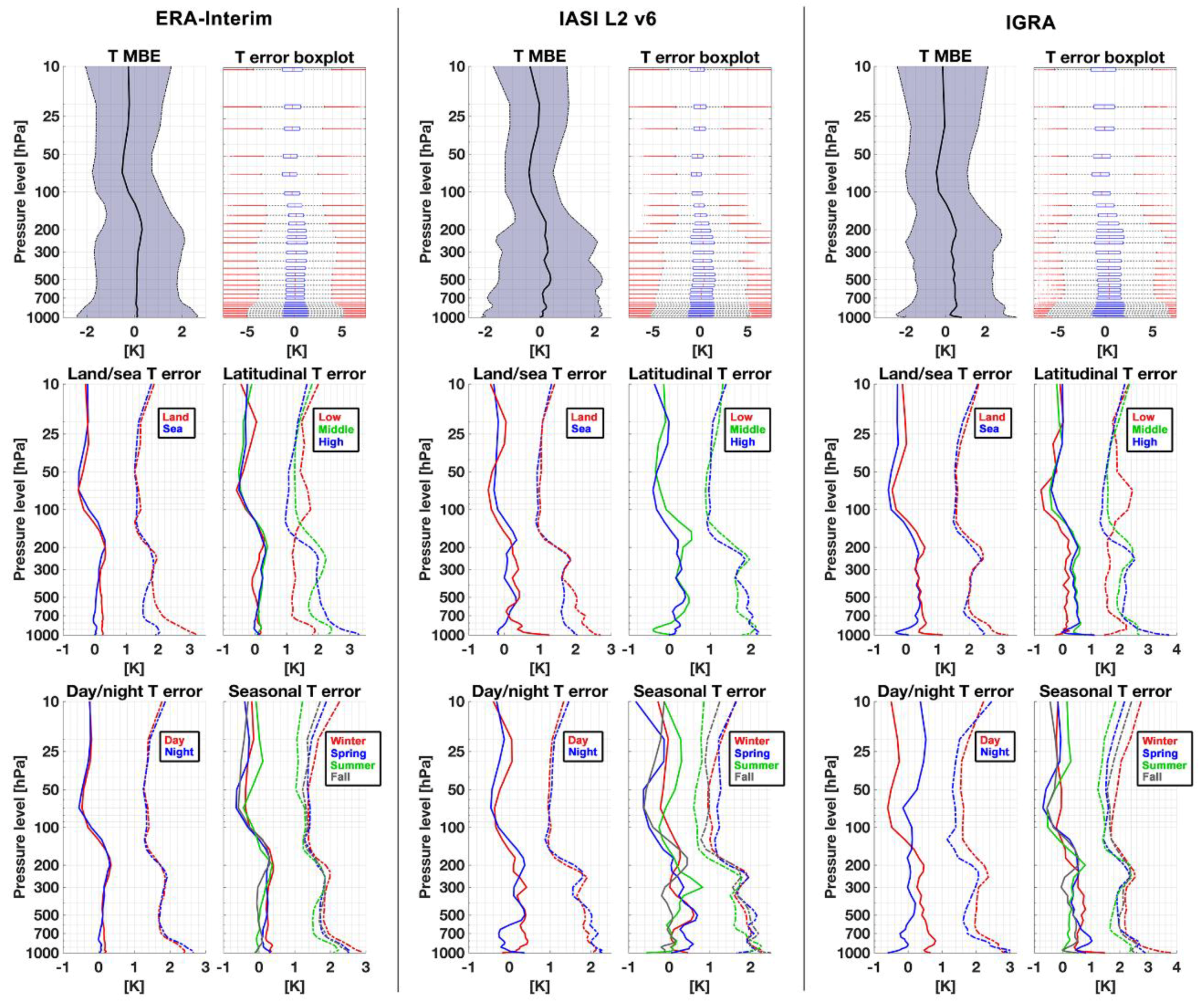
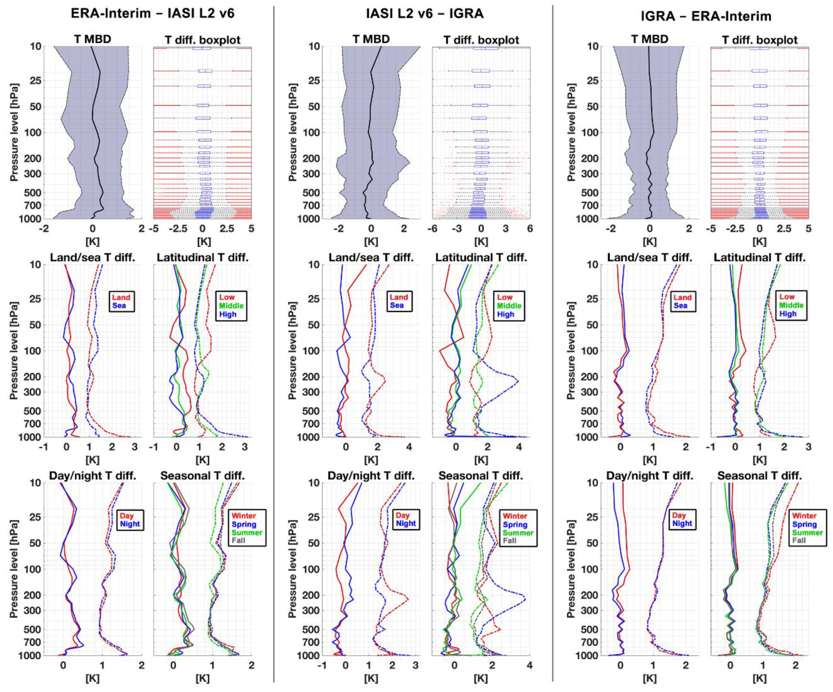
Appendix A. ERA-Interim, IASI L2 v6, and IGRA Intercomparisons

Figure A1 shows the T and Q mean vertical profiles with the standard deviation for ERA-Interim, IASI L2 v6, and IGRA separately. These profiles were obtained by using all the 2016 available data for ERA-Interim and IGRA, consisting of 5·106 and 5·105 samples respectively, and by using 107 IASI L2 v6 profiles randomly drawn from the full dataset of more than 1.8·108 samples. The trend of both T and Q vertical profiles seem quite regular and similar among the three data sources, although there are non-negligible differences, mostly near the surface. In fact, near the surface, ERA-Interim T is lower than IASI L2 v6 T and IGRA T up to ~10 K and ~5 K, respectively, while IASI L2 v6 Q is generally larger than ERA-Interim Q and IGRA Q by about 2 g/kg below the 800 hPa level. Furthermore, the IASI L2 v6 profile shows a minor Q inversion around 725 hPa. To better understand the differences among the three databases, the space and time colocated T and WV vertical profiles among ERA-Interim–IASI L2 v6, IASI L2 v6–IGRA, and IGRA–ERA-Interim were analyzed separately, for all the 2016 data. By using a one-minute delay, the IASI L2 v6 and IGRA vertical profiles were considered coincident with the ERA-Interim ones when the IASI IFOV center and the IGRA station were inside the (0.75 × 0.75)° box around the ERA-Interim grid point, while the IASI L2 v6 and IGRA vertical profiles were considered coincident when IGRA station was inside the IASI IFOV. The small number of the IASI L2 v6–IGRA profiles is due to the lack of space–time coincidences of the IGRA stations with the IASI overpass, combined with having only two years of IASI-L2 v6 product availability.
Figure A1. ERA-Interim, IASI L2 v6, and IGRA T (left) and Q (right) mean vertical profiles (solid) and standard deviation (dashed lines and shaded areas).
Remotesensing 10 01398 g0a1
Figure A2 (top panels) show the ERA-Interim, IASI L2 v6, and IGRA MBD and the standard deviations in a circular way; that is, the ERA-Interim–IASI L2 v6 T differences, the IASI L2 v6–IGRA T differences, and the IGRA–ERA-Interim T differences, with relative boxplots. In the middle and bottom panels of Figure A2, the MBD and the RMSD are shown separately for land/sea; for low, middle, and high latitude; for day/nighttime; and for the four seasons. Even if the three mean values with their standard deviations in the top panels are similar, the boxplot shows non-negligible differences in colocated T values, characterized by about 1 K for the interquartile range. Consistently with these values, the MBD are generally contained in the range −0.5–0.5 K, with the largest differences at high latitudes and low altitudes between IASI L2 v6 and IGRA. Furthermore, for low–middle altitudes, the IASI L2 v6 mean values are a little lower than IGRA and ERA-Interim ones. The RMSD is generally contained in the range 1–2 K, with larger values near the surface and smaller values around 500–600 hPa. The highest variations are for different latitudes and for land/sea surface, while day/nighttime, as well as the season, has slightly less impact on both MBD and RMSD. The smallest errors are generally for high latitude, land surface, and low altitudes. Among the three datasets, the largest differences are between IASI L2 v6–IGRA and ERA-Interim–IASI L2 v6, while IGRA and ERA-Interim seem more regular and similar to each other.
Figure A2. ERA-Interim, IASI L2 v6, and IGRA T intercomparisons. Top panels show mean bias difference (MBD) (solid) with standard deviations (dashed area) and the boxplot of the differences. Middle and bottom panels show MBD (solid lines) and root mean square difference (RMSD) (dashed lines) of the differences for land/sea surface, high/middle/low latitude, daytime/nighttime, and for the four seasons. ERA-Interim–IASI L2 v6, IASI L2 v6–IGRA, and IGRA–ERA-Interim are shown by the left, center, and right panels, respectively.
Remotesensing 10 01398 g0a2
The analysis for Q (Figure A3) shows similar results to those obtained for T, even if the former is more variable than the latter. The interquartile difference is about −0.75–0.75 g/kg, and both the MBD and RMSE show the maximum values generally at low latitudes, around 875 hPa when IASI L2 v6 is compared against both ERA-Interim and IGRA. The largest differences are in the ERA-Interim–IASI L2 v6 and IASI L2 v6–IGRA intercomparisons, while the IGRA and ERA-Interim datasets seem more homogeneous among them. The RMSD is maximum near 875 hPa for low latitude, while day/night, season, and land/sea effect do not produce evident effects.
Figure A3. ERA-Interim, IASI L2 v6, and IGRA Q intercomparisons. Top panels show MBD (solid) with standard deviations (dashed area) and the boxplot of the differences. The panels of the second and third rows show MBD (solid lines) and RMSD (dashed lines) of the differences for land/sea surface, high/middle/low latitude, daytime/nighttime, and for the four seasons. ERA-Interim–IASI L2 v6, IASI L2 v6–IGRA, and IGRA–ERA-Interim are shown by the left, center, and right panels, respectively.
Remotesensing 10 01398 g0a3

Appendix B. Mixing Ratio Calculation

To obtain Q starting from RH and T, the following formulas were used [66,67,68]:
  Q = 621.97   P q   P r e f P q
  P q = R H   100 P q s
where Pqs is the saturated vapor pressure, Pq is the water vapor pressure, and Pref is the reference pressure. To obtain Pqs, the Wagner and Pruß equation was used [69]:
  P q s   = P c exp   [   τ   ( α 1 θ + α 2 θ 1.5 + α 3 θ 1.5 + α 3 θ 3 + α 4 θ 3.5 + α 5 θ 4 + α 6 θ 7.5   ) ]
where Pc = 22.064002·107 Pa is the critical pressure, τ = Tc/T, θ = 1−T/Tc, α1 = −7.85951783, α2 = 1.84408259, α3 = −11.7866497, α4 = 22.6807411, α5 = −15.9618719, α6 = 1.80122502, and Tc = 647.096 K is the water critical-point temperature. Equation (A3) is valid in the temperature interval 273.16 K ≤ T ≤ 647 K; for this reason, the following formula was used below 273.16 K, claimed to be valid in the range 123K < T < 332K [70]:
P q s   = exp   [ β 1 + β 2 T + β 3 l n ( T ) + β 4 T + t a n h { β 5 ( T + β 6 ) } ( β 7 + β 8 T + β 9 l n ( T ) + β 10   T ) ]
where β1 = 54.842763, β2 = −6763.22, β3 = −4.21, β4 = 0.000367, β5 = 0.0415, β6 = −218.8, β7 = 53.878, β8 = −1331.22, β9 = −9.44523, β10 = 0.014025, tanh(·) denotes a hyperbolic tangent, and ln(·) is the natural logarithm.

References

  1. Liu, X.; Kizer, S.; Barnet, C.; Divakarla, M.; Gu, D.; Zhou, D.K.; Larar, A.M.; Xiong, X.; Guo, G.; Nalli, N.R.; et al. Retrieving Atmospheric Temperature and Moisture Profiles from Suomi NPP Cris/ATMS Sensors Using Crimss EDR Algorithm. In Proceedings of the 2012 IEEE International Geoscience and Remote Sensing Symposium, Munich, Germany, 22–27 July 2012; pp. 1956–1959. [Google Scholar] [CrossRef]
  2. Di Paola, F.; Dietrich, S. Resolution enhancement for microwave-based atmospheric sounding from geostationary orbits. Radio Sci. 2008, 43, RS6001. [Google Scholar] [CrossRef]
  3. Kwon, E.; Sohn, B.J.; Smith, W.L.; Li, J. Validating IASI Temperature and Moisture Sounding Retrievals over East Asia Using Radiosonde Observations. J. Atmos. Ocean. Technol. 2012, 29, 1250–1262. [Google Scholar] [CrossRef]
  4. Singh, R.; Kishtawal, C.M.; Pal, P.K.; Joshi, P.C. Improved tropical cyclone forecasts over north Indian Ocean with direct assimilation of AMSU-A radiances. Meteorol. Atmos. Phys. 2012, 115, 15–34. [Google Scholar] [CrossRef]
  5. Bony, S.; Colman, R.; Kattsov, V.M.; Allan, R.P.; Bretherton, C.S.; Dufresne, J.-L.; Hall, A.; Hallegatte, S.; Holland, M.M.; Ingram, W.; et al. How well do we understand and evaluate climate change feedback processes? J. Clim. 2006, 19, 3445–3482. [Google Scholar] [CrossRef]
  6. Soden, B.J.; Held, I.M. An assessment of climate feedbacks in coupled ocean-atmosphere models. J. Clim. 2006, 19, 3354–3360. [Google Scholar] [CrossRef]
  7. Santer, B.D.; Sausen, R.; Wigley, T.M.L.; Boyle, J.S.; Achuta Rao, K.; Doutriaux, C.; Hansen, J.E.; Meehl, G.A.; Roeckner, E.; Ruedy, R.; et al. Behavior of tropopause height and atmospheric temperature in models, reanalyses, and observations: Decadal changes. J. Geophys. Res. 2003, 108, 4002. [Google Scholar] [CrossRef]
  8. Barker, D.; Huang, X.; Liu, Z.; Auligné, T.; Zhang, X.; Rugg, S.; Ajjaji, R.; Bourgeois, A.; Bray, J.; Chen, Y.; et al. The Weather Research and Forecasting Model’s Community Variational/Ensemble Data Assimilation System: WRFDA. Bull. Am. Meteorol. Soc. 2012, 93, 831–843. [Google Scholar] [CrossRef]
  9. Li, J.; Li, J.; Schmit, T.J.; Otkin, J.; Liu, C.-Y. Warning information in preconvection environment from geostationary advanced infrared sounding system—A simulation study using the IHOP case. J. Appl. Meteorol. Climatol. 2011, 50, 766–783. [Google Scholar] [CrossRef]
  10. Li, J.; Liu, H. Improved hurricane track and intensity forecast using single field-of-view advanced IR sounding measurements. Geophys. Res. Lett. 2009, 36, L11813. [Google Scholar] [CrossRef]
  11. Liu, H.; Li, J. An improved in forecasting rapid intensification of Typhoon Sinlaku (2008) using clear-sky full spatial resolution advanced IR soundings. J. Appl. Meteorol. Climatol. 2010, 49, 821–827. [Google Scholar] [CrossRef]
  12. Zou, X.; Weng, F.; Zhang, B.; Lin, L.; Qin, Z.; Tallapragada, V. Impacts of assimilation of ATMS data in HWRF on track and intensity forecasts of 2012 four landfall hurricanes. J. Geophys. Res. Atmos. 2013, 118, 11558–11576. [Google Scholar] [CrossRef]
  13. Gangwar, R.K.; Mathur, A.K.; Gohil, B.S.; Basu, S. Neural Network Based Retrieval of Atmospheric Temperature Profile Using AMSU-A Observations. Int. J. Atmos. Sci. 2014, 8. [Google Scholar] [CrossRef]
  14. Rosenkranz, P.W.; Komichak, M.J.; Staelin, D.H. A Method for Estimation of Atmospheric Water Vapor Profiles by Microwave Radiometry. J. Appl. Meteorol. 1982, 21, 1364–1370. [Google Scholar] [CrossRef] [Green Version]
  15. Kakar, R.K.; Lambrigtsen, B.H. A Statistical Correlation Method for the Retrieval of Atmospheric Moisture Profiles by Microwave Radiometry. J. Climate Appl. Meteorol. 1984, 23, 1110–1114. [Google Scholar] [CrossRef] [Green Version]
  16. Cabrera-Mercadier, C.; Staelin, D. Passive microwave relative humidity retrievals using feedforward neural networks. IEEE Trans. Geosci. Remote Sens. 1995, 33, 1324–1328. [Google Scholar] [CrossRef]
  17. Shi, L. Retrieval of atmospheric temperature profiles from AMSU-A measurements using a neural network approach. J. Atmos. Ocean. Technol. 2001, 18, 340–347. [Google Scholar] [CrossRef]
  18. Aires, F.; Prigent, C.; Rossow, W.B.; Rothstein, M. A new neural network approach including first guess for retrieval of atmospheric water vapor, cloud liquid water path, surface temperature, and emissivities over land from satellite microwave observations. J. Geophys. Res. 2001, 106, 14887–14907. [Google Scholar] [CrossRef] [Green Version]
  19. Karbou, F.; Aires, F.; Prigent, C.; Eymard, L. Potential of Advanced Microwaves Sounding Unit-A (AMSU-A) and AMSU-B measurements for atmospheric temperature and humidity profiling over land. J. Geophys. Res. 2005, 110, D07109. [Google Scholar] [CrossRef]
  20. Wang, J.R.; Chang, L.A. Retrieval of Water Vapor Profiles from Microwave Radiometric Measurements near 90 and 183 GHz. J. Appl. Meteorol. 1990, 29, 1005–1013. [Google Scholar] [CrossRef] [Green Version]
  21. Blankenship, C.B.; Al-Khalaf, A.; Wilheit, T.T. Retrieval of Water Vapor Profiles Using SSM/T-2 and SSM/I Data. J. Atmos. Sci. 2000, 57, 939–955. [Google Scholar] [CrossRef]
  22. Rosenkranz, P.W. Retrieval of temperature and moisture profiles from AMSU-A and AMSU-B measurements. IEEE Trans. Geosci. Remote Sens. 2001, 39, 2429–2435. [Google Scholar] [CrossRef]
  23. Boukabara, S.-A.; Garrett, K.; Chen, W.; Iturbide-Sanchez, F.; Grassotti, C.; Kongoli, C.; Chen, R.; Liu, Q.; Yan, B.; Weng, F.; et al. MiRS: An all-weather 1DVAR satellite data assimilation and retrieval system. IEEE Trans. Geosci. Remote Sens. 2011, 49, 3249–3272. [Google Scholar] [CrossRef]
  24. Romano, F.; Cimini, D.; Nilo, S.T.; Di Paola, F.; Ricciardelli, E.; Ripepi, E.; Viggiano, M. The Role of Emissivity in the Detection of Arctic Night Clouds. Remote Sens. 2017, 9, 406. [Google Scholar] [CrossRef]
  25. Romano, F.; Ricciardelli, E.; Cimini, D.; Di Paola, F.; Viggiano, M. Dust Detection and Optical Depth Retrieval Using MSG-SEVIRI Data. Atmosphere 2013, 4, 35–47. [Google Scholar] [CrossRef]
  26. Gallucci, D.; Romano, F.; Cersosimo, A.; Cimini, D.; Di Paola, F.; Gentile, S.; Geraldi, E.; Larosa, S.; Nilo, S.T.; Ricciardelli, E.; et al. Nowcasting Surface Solar Irradiance with AMESIS via Motion Vector Fields of MSG-SEVIRI Data. Remote Sens. 2018, 10, 845. [Google Scholar] [CrossRef]
  27. Weng, F.; Zou, X.; Wang, X.; Yang, S.; Goldberg, M.D. Introduction to Suomi national polar-orbiting partnership advanced technology microwave sounder for numerical weather prediction and tropical cyclone applications. J. Geophys. Res. 2012, 117, D19112. [Google Scholar] [CrossRef]
  28. Zabolotskikh, E.V. Contemporary methods for retrieving the integrated atmospheric water-vapor content and the total cloud liquid-water content. Izv. Atmos. Ocean. Phys. 2017, 53, 294–300. [Google Scholar] [CrossRef]
  29. Zheng, J.; Li, J.; Schmit, T.; Li, J.; Liu, Z. The impact of AIRS atmospheric temperature and moisture profiles on hurricane forecasts: Ike (2008) and Irene (2011). Adv. Atmos. Sci. 2015, 32, 319–335. [Google Scholar] [CrossRef]
  30. Breiman, L. Random forests. Mach. Learn. 2001, 45, 5–32. [Google Scholar] [CrossRef]
  31. Svetnik, V.; Liaw, A.; Tong, C.; Culberson, J.C.; Sheridan, R.P.; Feuston, B.P. Random Forest: A Classification and Regression Tool for Compound Classification and QSAR Modeling. J. Chem. Inf. Comput. Sci. 2003, 43, 1947–1958. [Google Scholar] [CrossRef] [PubMed]
  32. Berrisford, P.; Dee, D.; Poli, P.; Brugge, R.; Fielding, K.; Fuentes, M.; Kallberg, P.; Kobayashi, S.; Uppala, S.; Simmons, A. The ERA-Interim Archive, Version 2.0; ERA Report Series; Technical Report; ECMWF: Reading, UK, 2011; p. 23. [Google Scholar]
  33. Dee, D.P.; Uppala, S.M.; Simmons, A.J.; Berrisford, P.; Poli, P.; Kobayashi, S.; Andrae, U.; Balmaseda, M.A.; Balsamo, G.; Bauer, P.; et al. The ERA-Interim reanalysis: Configuration and performance of the data assimilation system. Q. J. R. Meteorol. Soc. 2011, 137, 553–597. [Google Scholar] [CrossRef]
  34. Schlüessel, P.; Hultberg, T.H.; Phillips, P.L.; August, T.; Calbet, X. The operational IASI Level 2 processor. Adv. Space Res. 2005, 36, 982–988. [Google Scholar] [CrossRef] [Green Version]
  35. August, T.; Klaes, D.; Schlüssel, P.; Hultberg, T.; Crapeau, M.; Arriaga, A.; O’Carroll, A.; Coppens, D.; Munro, R.; Calbet, X. IASI on Metop-A: Operational level 2 retrievals after five years in orbit. J. Quant. Spectrosc. Radiat. Transf. 2012, 113, 1340–1371. [Google Scholar] [CrossRef]
  36. Durre, I.; Vose, R.S.; Wuertz, D.B. Overview of the Integrated Global Radiosonde Archive. J. Clim. 2006, 19, 53–68. [Google Scholar] [CrossRef] [Green Version]
  37. Durre, I.; Yin, X. Enhanced radiosonde data for studies of vertical structure. Bull. Am. Meteorol. Soc. 2008, 89, 1257–1262. [Google Scholar] [CrossRef]
  38. Hortal, M.; Simmons, A.J. Use of reduced Gaussian grids in spectral models. Mon. Weather Rev. 1991, 119, 1057–1074. [Google Scholar] [CrossRef]
  39. Roman, J.; Knuteson, R.; August, T.; Hultberg, T.; Ackerman, S.; Revercomb, H. A global assessment of NASA AIRS v6 and EUMETSAT IASI v6 precipitable water vapor using ground-based GPS SuomiNet stations. J. Geophys. Res. Atmos. 2016, 121, 8925–8948. [Google Scholar] [CrossRef]
  40. Dietrich, S.; Casella, D.; Di Paola, F.; Formenton, M.; Mugnai, A.; Sanò, P. Lightning-based propagation of convective rain fields. Nat. Hazards Earth Syst. Sci. 2011, 11, 1571–1581. [Google Scholar] [CrossRef] [Green Version]
  41. Munoz, E.A.; Di Paola, F.; Lanfri, M. Advances on Rain Rate Retrieval from Satellite Platforms using Artificial Neural Networks. IEEE Lat. Am. Trans. 2015, 13, 3179–3186. [Google Scholar] [CrossRef]
  42. Munoz, E.A.; Di Paola, F.; Lanfri, M.; Arteaga, F.J. Observing the Troposphere through the Advanced Technology Microwave Sensor (ATMS) to Retrieve Rain Rate. IEEE Lat. Am. Trans. 2016, 14, 586–594. [Google Scholar] [CrossRef]
  43. Sanò, P.; Panegrossi, G.; Casella, D.; Marra, A.C.; Di Paola, F.; Dietrich, S. The new Passive microwave Neural network Precipitation Retrieval (PNPR) algorithm for the cross-track scanning ATMS radiometer: Description and verification study over Europe and Africa using GPM and TRMM spaceborne radars. Atmos. Meas. Tech. 2016, 9, 5441–5460. [Google Scholar] [CrossRef]
  44. Zou, X.; Lin, L.; Weng, F. Absolute Calibration of ATMS Upper Level Temperature Sounding Channels Using GPS RO Observations. IEEE Trans. Geosci. Remote Sens. 2014, 52, 1397–1406. [Google Scholar] [CrossRef]
  45. Hastie, T.; Tibshirani, R.; Friedman, J. The Elements of Statistical Learning; Springer: New York, NY, USA, 2001. [Google Scholar]
  46. Breiman, L.; Friedman, J.H.; Olshen, R.A.; Stone, C.J. Classification and Regression Trees; Routledge, Wadsworth International Group: Belmont, CA, USA, 1984. [Google Scholar]
  47. Dietterich, T.G. Machine learning for sequential data: A review. In Structural, Syntactic, and Statistical Pattern Recognition; Caelli, T., Ed.; Volume 2396 of Lecture Notes in Computer Science; Springer: Berlin/Heidelberg, Germany, 2002; pp. 15–30. [Google Scholar]
  48. Breiman, L. Bagging Predictors. In Machine Learning; Springer: Berlin/Heidelberg, Germany, 1996; Volume 24, pp. 123–140. [Google Scholar]
  49. Ricciardelli, E.; Cimini, D.; Di Paola, F.; Romano, F.; Viggiano, M. A statistical approach for rain intensity differentiation using Meteosat Second Generation–Spinning Enhanced Visible and InfraRed Imager observations. Hydrol. Earth Syst. Sci. 2014, 18, 2559–2576. [Google Scholar] [CrossRef] [Green Version]
  50. Mitchell, M.W. Bias of the random forest out-of-bag (OOB) error for certain input parameters. Open J. Stat. 2011, 1, 205–211. [Google Scholar] [CrossRef]
  51. Mugnai, A.; Smith, E.A.; Tripoli, G.J.; Bizzarri, B.; Casella, D.; Dietrich, S.; Di Paola, F.; Panegrossi, G.; Sanò, P. CDRD and PNPR satellite passive microwave precipitation retrieval algorithms: EuroTRMM/EURAINSAT origins and HSAF operations. Nat. Hazards Earth Syst. Sci. 2013, 13, 887–912. [Google Scholar] [CrossRef]
  52. Chen, F.W.; Staelin, D.H. AIRS/AMSU/HSB Precipitation Estimates. IEEE Trans. Geosci. Remote Sens. 2003, 41, 410–417. [Google Scholar] [CrossRef]
  53. Hashemi, M. Reusability of the Output of Map-Matching Algorithms Across Space and Time through Machine Learning. IEEE Trans. Intell. Transp. Syst. 2017, 18, 3017–3026. [Google Scholar] [CrossRef]
  54. Aquino, L.D.; Tullis, J.A.; Stephen, F.M. Modeling red oak borer, Enaphalodes rufulus (Haldeman), damage using in situ and ancillary landscape data. For. Ecol. Manag. 2008, 255, 931–939. [Google Scholar] [CrossRef]
  55. Liaw, A.; Wiener, M. Classification and regression by randomForest. R News 2002, 2/3, 18–22. [Google Scholar]
  56. Segal, M.R. Machine Learning Benchmarks and Random Forest Regression. In eScholarship Repository; University of California: Berkeley, San Francisco, CA, USA, 2003; Available online: http://repositories.cdlib.org/cbmb/bench_rf_regn (accessed on 1 August 2018).
  57. Boulesteix, A.; Janitza, S.; Kruppa, J.; König, I.R. Overview of random forest methodology and practical guidance with emphasis on computational biology and bioinformatics. Wiley Interdiscip. Rev. Data Min. Knowl. Discov. 2012, 2, 493–507. [Google Scholar] [CrossRef] [Green Version]
  58. Roy, M.-H.; Larocque, D. Robustness of random forests for regression. J. Nonparametr. Stat. 2012, 24, 993–1006. [Google Scholar] [CrossRef]
  59. Chevallier, F.; Di Michele, S.; McNally, A.P. Diverse Profile Datasets from the ECMWF 91-Level Short-Range Forecasts; Report NWPSAF-EC-TR-010; European Centre for Medium-Range Weather Forecasts: Reading, UK, 2006. [Google Scholar]
  60. Gislason, P.O.; Benediktsson, J.A.; Sveinsson, J.R. Random Forests for land cover classification. Pattern. Recognit. Lett. 2006, 27, 294–300. [Google Scholar] [CrossRef]
  61. Vallance, L.; Charbonnier, B.; Paul, N.; Dubost, S.; Blanc, P. Towards a standardized procedure to assess solar forecast accuracy: A new ramp and time alignment metric. Sol. Energy 2017, 150, 408–422. [Google Scholar] [CrossRef]
  62. McGill, R.; Tukey, J.W.; Larsen, W.A. Variations of Box Plots. Am. Stat. 1978, 32, 12–16. [Google Scholar] [CrossRef]
  63. Boukabara, S.-A.; Garrett, K.; Grassotti, C.; Iturbide-Sanchez, F.; Chen, W.; Jiang, Z.; Clough, S.A.; Zhan, X.; Liang, P.; Liu, Q.; et al. A physical approach for a simultaneous retrieval of sounding, surface, hydrometeor, and cryospheric parameters from SNPP/ATMS. J. Geophys. Res. Atmos. 2013, 118, 12600–12619. [Google Scholar] [CrossRef]
  64. Nalli, N.R.; Gambacorta, A.; Liu, Q.; Barnet, C.D.; Tan, C.; Iturbide-Sanchez, F.; Reale, T.; Sun, B.; Wilson, M.; Borg, L.; et al. Validation of Atmospheric Profile Retrievals from the SNPP NOAA-Unique Combined Atmospheric Processing System. Part 1: Temperature and Moisture. IEEE Trans. Geosci. Remote Sens. 2018, 56, 180–190. [Google Scholar] [CrossRef]
  65. Nalli, N.R.; Barnet, C.D.; Reale, A.; Tobin, D.; Gambacorta, A.; Maddy, E.S.; Joseph, E.; Sun, B.; Borg, L.; Mollner, A.K.; et al. Validation of satellite sounder environmental data records: Application to the Cross-track Infrared Microwave Sounder Suite. J. Geophys. Res. Atmos. 2016, 118, 13628–13643. [Google Scholar] [CrossRef]
  66. Wexler, A. Vapor Pressure Formulation for Water in Range 0 to 100 °C. A Revision. J. Res. Natl. Bur. Stand. A 1976, 80, 775–785. [Google Scholar] [CrossRef]
  67. Bolton, D. The computation of equivalent potential temperature. Mon. Weather Rev. 1980, 108, 1046–1053. [Google Scholar] [CrossRef]
  68. Lawrence, M. The relationship between relative humidity and the dewpoint temperature in moist air: A simple conversion and applications. Bull. Am. Meteorol. Soc. 2005, 86, 225–233. [Google Scholar] [CrossRef]
  69. Wagner, W.; Pruß, A. The IAPWS Formulation 1995 for the Thermodynamic Properties of Ordinary Water Substance for General and Scientific Use. J. Phys. Chem. Ref. Data 2002, 31, 387–535. [Google Scholar] [CrossRef]
  70. Murphy, D.M.; Koop, T. Review of the vapor pressures of ice and supercooled water for atmospheric applications. Q. J. R. Meteorol. Soc. 2005, 131, 1539–1565. [Google Scholar] [CrossRef]
Figure 1. Location of the stations considered in the Integrated Global Radiosonde Archive (IGRA) database and involved in the training procedures.
Remotesensing 10 01398 g001
Figure 2. Flowchart of the action performed to develop the algorithm detailed in Section 3. Q: Water vapor mixing ratio, T: Temperature, RF: random forest, Nt: number of trees in the forest, Np: number of randomly selected predictors, Ms: minimum size of the terminal node.
Remotesensing 10 01398 g002
Figure 3. Predictor importance analysis for T (top) and Q (bottom) at three representative levels: 200 hPa (left), 500 hPa (center), and 900 hPa (right).
Remotesensing 10 01398 g003
Figure 4. Predictor selection and Np parameter analysis for T (top) and Q (bottom) at three representative levels: 200 hPa (left), 500 hPa (center), and 900 hPa (right). The panels also show the out-of-bag (OOB) root mean square error (RMSE) minimum values found (white crosses) and the chosen OOB RMSE minimum, corresponding to the lowest value of Np (white circle).
Remotesensing 10 01398 g004
Figure 5. Nt parameter analysis for T (left) and Q (right) at three representative levels (top to bottom: 900, 500, and 200 hPa). The cross-circle markers indicate the selected values of the Nt parameter.
Remotesensing 10 01398 g005
Figure 6. Ms parameter analysis for T (left) and Q (right) at three representative levels (top to bottom: 900, 500, and 200 hPa). The cross-circle markers indicate the selected values of the Ms parameter.
Remotesensing 10 01398 g006
Figure 7. Left: Estimated profile of T mean (solid) and standard deviation (STD) (shaded) for 2017. Center: profiles of the corresponding mean bias error (MBE). Right: profiles of the corresponding RMSE (dashed lines) compared with STD (solid lines).
Remotesensing 10 01398 g007
Figure 8. Top panels: T MBE with the STD and error boxplots for ERA-Interim (left), IASI L2 v6 (center), and IGRA (right) separately. Middle and bottom panels show MBE (solid lines) and RMSE (dashed lines) for land/sea surface, high/middle/low latitude, day/night, and the four seasons. The 2017 validation dataset is used to compute the statistics.
Remotesensing 10 01398 g008
Figure 9. Left: Estimated profile of Q mean (solid) and STD (shaded) for 2017. Center: profiles of the corresponding MBE. Right: profiles of the corresponding RMSE (dashed lines) compared with STD (solid lines).
Remotesensing 10 01398 g009
Figure 10. Top panels: Q MBE with the standard deviations and errors boxplot for ERA-Interim (left), IASI L2 v6 (center), and IGRA (right) separately. Middle and bottom panels show MBE (solid lines) and RMSE (dashed lines) for land/sea surface, high/middle/low latitude, day/night, and the four seasons. The 2017 validation dataset is used to compute the statistics.
Remotesensing 10 01398 g010
Table 1. ATMS (1) channel characteristics.
ChannelCentral Frequency [GHz]Beam Width [deg]Resolution at s.s.p. (2) [km]NEΔT (3) [K]Peak WF (4) [mb]
123.85.2∼750.51085.394
231.45.2∼750.61085.394
350.32.2∼320.71085.394
451.762.2∼320.51085.394
552.82.2∼320.5891.7679
653.596 ± 0.1152.2∼320.5606.847
754.42.2∼320.5351.237
854.942.2∼320.5253.637
955.52.2∼320.5165.241
1057.29032.2∼320.7586.337
1157.2903 ± 0.2172.2∼321.049.326
1257.2903 ± 0.322 ± 0.0482.2∼321.024.793
1357.2903 ± 0.322 ± 0.0222.2∼321.510.240
1457.2903 ± 0.322 ± 0.0102.2∼322.25.385
1557.2903 ± 0.322 ± 0.0042.2∼323.63.010
1688.22.2∼320.31085.394
17165.51.1∼160.61085.394
18183.31 ± 71.1∼160.8790.017
19183.31 ± 4.51.1∼160.8695.847
20183.31 ± 31.1∼160.8606.847
21183.31 ± 1.81.1∼160.8506.115
22183.31 ± 11.1∼160.9450.738
Note: (1) Advanced Technology Microwave Sounder; (2) Sub-satellite point; (3) Noise equivalent ΔT; (4) Weighting function.
Table 2. Main characteristics of the data considered in this study.
NameSizeFormatPeriodSpatial ResolutionTemporal Resolutions# Profile per Year
ERA-Interim~500 GbGRIB2012–2017(0.75 × 0.75)°4 simulation per day~1.6 × 10⁸
IASI L2 v6~2 TbNetCDF2015–201712 km (s.s.p.)~28 orbits per day~8.5·× 108
IGRA~5 KbASCII2012–2017punctual2 or 4 measures per day~4.7·× 105
ATMS~1 TbHDF2012–201716 km (s.s.p.)~14 orbits per day~1.1·× 109
Table 3. Predictors definition for the RF training purpose.
Short NamePredictor
p1–p22ATMS BT ch. 1–22 [K]
p23ATMS scan angle [deg]
p24latitude [deg]
p25sin(longitude)
p26cos(longitude)
p27land/sea flag
p28sin(2p·DOY (1)/365)
p29cos(2p·DOY/365)
p30solar zenith angle [deg]
Note: (1) day-of-year.
Table 4. Summary of predictors and parameters used to train the RFs. T profiles are defined within 10–1000 hPa, while WV profiles are defined within 200–1000 hPa.
LevelTWV
PredictorsNpNtMsPredictorsNpNtMs
10 hPap5 ÷ p15, p23 ÷ p24, p28 ÷ p29121902
20 hPap5 ÷ p15, p17, p23 ÷ p24, p28, p29112801
30 hPap4 ÷ p15, p17 ÷ p18, p23 ÷ p24, p28 ÷ p30113201
50 hPap4 ÷ p15, p17 ÷ p18, p23 ÷ p24, p28 ÷ p29102601
70 hPap3 ÷ p15, p17 ÷ p21, p23 ÷ p26, p28 ÷ p30172501
100 hPap3 ÷ p15, p17 ÷ p21, p23 ÷ p26, p28 ÷ p30162302
125 hPap4 ÷ p15, p17 ÷ p19, p21 ÷ p24, p26, p28 ÷ p29143201
150 hPap4 ÷ p15, p17 ÷ p19, p22 ÷ p25, p28 ÷ p29172601
175 hPap5 ÷ p14, p23 ÷ p24, p2891702
200 hPap5 ÷ p13, p23 ÷ p24, p2883301p1 ÷ p30112003
225 hPap4 ÷ p15, p17, p22 ÷ p26, p28 ÷ p29162502p1 ÷ p30183202
250 hPap4 ÷ p14, p17 ÷ p18, p21 ÷ p26, p28, p29152501p1 ÷ p30194402
300 hPap1 ÷ p30203801p1 ÷ p30213902
350 hPap1 ÷ p30203801p1 ÷ p30173101
400 hPap1 ÷ p30202201p1 ÷ p30133101
450 hPap1 ÷ p30204601p1 ÷ p30174001
500 hPap1 ÷ p30204102p1 ÷ p30163801
550 hPap1 ÷ p30183101p1 ÷ p30162202
600 hPap1 ÷ p30183301p1 ÷ p30172701
650 hPap1 ÷ p30213301p1 ÷ p30182102
700 hPap1 ÷ p30172901p1 ÷ p30173801
750 hPap1 ÷ p30144401p1 ÷ p30123602
775 hPap1 ÷ p30182701p1 ÷ p30132201
800 hPap1 ÷ p30182602p1 ÷ p30172601
825 hPap1 ÷ p30163701p1 ÷ p30133201
850 hPap1 ÷ p30133501p1 ÷ p30173602
875 hPap1 ÷ p30152701p1 ÷ p30162701
900 hPap1 ÷ p30183201p1 ÷ p30183301
925 hPap1 ÷ p30162901p1 ÷ p30186201
950 hPap1 ÷ p30213701p1 ÷ p30166001
975 hPap1 ÷ p30162501p1 ÷ p30153401
1000 hPap1 ÷ p30222501p1 ÷ p30213502

