Sea Surface Temperature (SST) Variability of the Eastern Coastal Zone of the Gulf of California

Abstract

The coastal zones are areas with a high flow of energy and materials where diverse ecosystems are developed. The study of coastal oceanography is important to understand the variability of these ecosystems and determine their role in biogeochemical cycles and climate change. Sea surface temperature (SST) analysis is indispensable for the characterization of physical and biological processes, and it is affected by processes at diverse timescales. The purpose of this work is to analyze the oceanographic variability of the Eastern Coastal Zone of the Gulf of California through the study of the SST from time series analysis of monthly data obtained from remote sensors (AVHRR-Pathfinder Version 5.1 and Version 5 resolution of 4 km, MODIS-Aqua, resolution of 4 km) for the period 1981 to 2016. The descriptive analysis of SST series showed that the values decrease from south to north, as well as the amplitude of the warm period decrease from south to north (cold period increase from south to north). The minimum values occurred during January and February, and ranged between 18 and 20 °C; and maximum values, of about 32 °C, arose in August and September. Cluster analysis allowed to group the data in four regions (south, center, midriff islands and north), the spectral analysis in each region showed frequencies of variation in scales: Annual (the main), seasonal, semiannual, and interannual. The latter is associated with the El Niño and La Niña climatological phenomena.

1. Introduction

The coastal zones are wide geographical areas with intense physical, chemical and biological interactions with strong exchange of energy and materials between the terrestrial environment, aquatic environment and the atmosphere [1]. The coastal zones have high primary productivity levels and play important role in the biogeochemical cycles [2]. These areas support high abundance of natural resources, providing refuge, feeding and spawning areas for diverse organisms, and enhancing activities like tourism, aquaculture and fisheries [3].

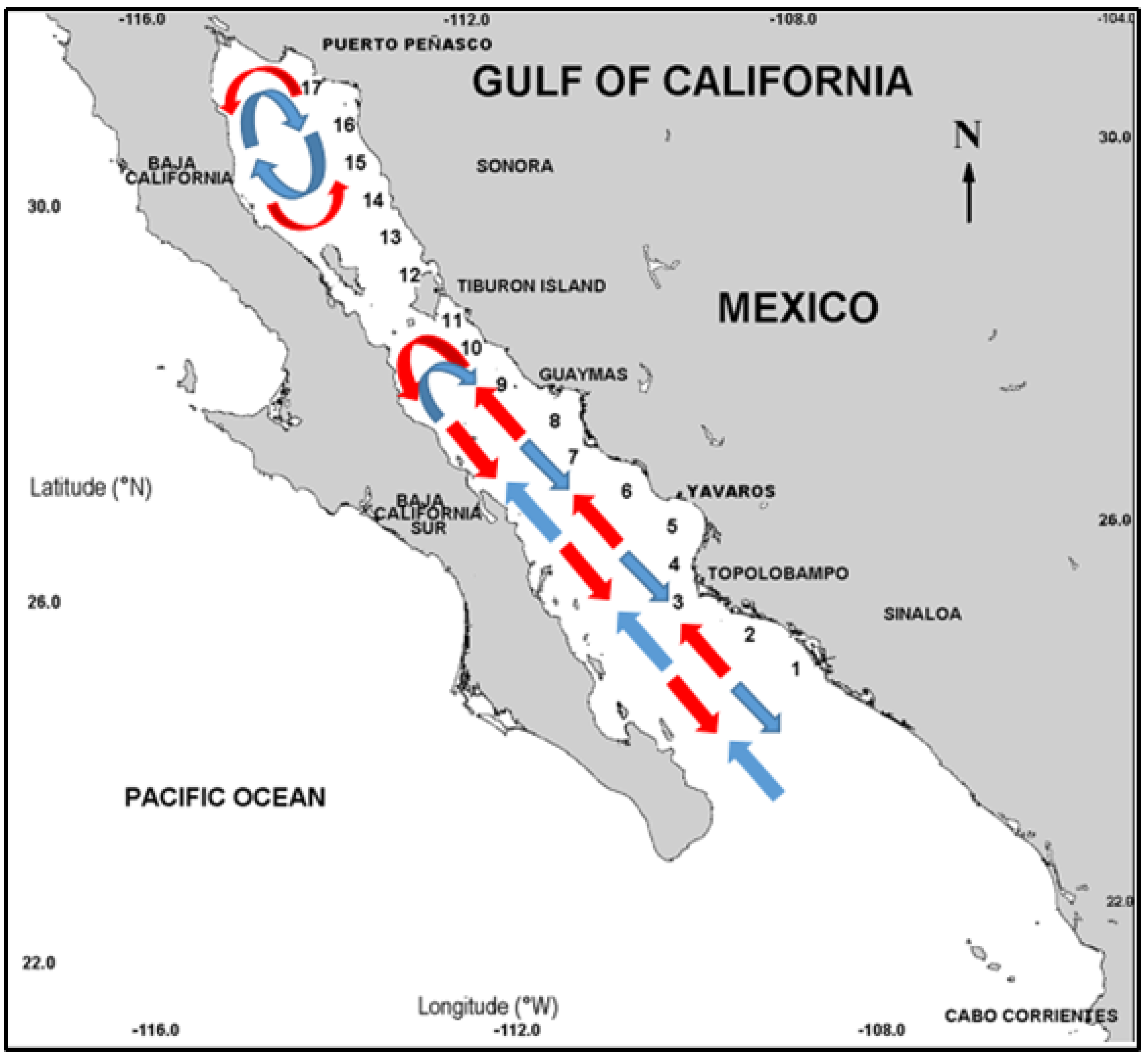
The Gulf of California is a marginal sea located in the Eastern Pacific Ocean, surrounded by arid environment that encompasses the Baja California Peninsula, and the states of Sonora, Sinaloa, and Nayarit, with an average length and width of 1400 and 150–200 km respectively and basins (deepening to the south) separated by sills [4,5]. Tidal currents, the transfer of wind moment, upwelling and high solar heating determine a strong physical dynamics [5]. Northwest Winds from December to May produce intense upwelling processes off the Eastern Coast. During these “winter conditions”, nutrients supply enhance the growth of phytoplankton communities. While, from July to October, the prevailing winds from the southeast, are weak and do not have enough energy to break the strong thermal stratification of the water column in summer, these “summer conditions” do not have an effect on the levels of phytoplankton biomass on the western coast [5,6]. The months of June and November are considered periods of transition between both conditions [7]. On the other hand, the Baja California Peninsula has mountain ranges that prevent the low-level clouds from the Pacific Ocean influencing in the gulf generating cloud-free most of the time with exceptions in summer when the tropical air from the south moves into the gulf [8].

The Eastern Coast of the Gulf of California is characterized by diverse water bodies, that play an important role in fisheries. This coastal zone has a coastal plain with an extensive deltaic river formed by the Colorado, Sonora, Yaqui and Mayo Rivers [9]. The seasonal coastal winds develop a sea surface circulation along the coast, to the south during October–March, and to the north during June–September [8,10].

Sea surface temperature (SST) is considered the most important variable in oceanography, it is considered an essential climate variable (ECV) and essential ocean variable (EOV) [11], because influences many physical, chemical and biological properties of oceans, and is an effective indicator of changes in marine ecosystems [12]. SST is considered the most important variable in oceanography. The SST temporal spatial distribution is useful in the location of thermal fronts, current systems in the oceans and the exchange of thermal energy between the ocean and the atmosphere [13]. In the recent years, the anthropogenic activities have increased contributing to climate change through modifications of physical and chemical aspects in the marine ecosystems [14,15]. Global warming associated with anthropogenic climate change impacts both mean SST, and as well as the thermal and atmospheric processes that affect ocean circulations. It also has influence on the physiology, behavior and demographic aspects of organism, altering size, structure, range of distribution, and abundance of populations consequently generating changes the trophic routes and the community and functions of the ecosystem [15]. The changes in the SST have as a consequence, alterations in the marine biological processes, from individuals to ecosystems, in local to global scales, impacting the ecosystem services [16]. The SST as an ECV is of great importance for the study, monitoring and management of the marine environment since it allows to quantitatively estimate recent changes and their effect on ecosystem services [12].

When analyzing SST variability, it is important to study its trends of change associated with environmental modifications that can occur of a natural or anthropogenic form [17]. From this perspective, remote sensing is a technique that can provide a high temporal resolution with a wide coverage of environmental variables; besides, their cost is lower than in situ measurements from boats that are not considered optimal when looking for long and large regions. The use of satellite images, through remote sensing, has allowed having accurate information on a global scale describing the physical and biological aspects of the oceans [18]. One of the disadvantages of remote sensors are uncertainty of SST retrievals in the presence of clouds, atmospheric gases and aerosols [19]. The analysis of SST in marine environments can be a challenge due to the variety of available remote sensors characteristics and resolution (spatial, spectral, radiometric and temporal). The coastal areas are sites with large spatial and temporal fluctuations, showing a high complexity, their study requires the analysis of high-resolution processes [20,21]. Remote sensing provides adequate resolution of SST, a very important variable in oceanography that contributes to their long-term studies [20].

Several time series analyses have shown that sea surface temperature in the Gulf of California varies on seasonal to interannual scales [22,23]. Soto-Mardones et al. [22] found a decrease in the sea surface temperature from south to north, and also that the annual scale is responsible for most of the SST variability oscillating in phase with minor north-south variations. Escalante et al. [24] also reported this decrease of the SST average from south to north along the Gulf of California, with clear differences between the warm (summer and autumn) and cold (winter and spring) conditions for the entire gulf. Robles and Marinone [25], as well as Ripa and Marinone [26] found a clear seasonal SST variability across the Guaymas Basin in the Central Gulf of California: Winter conditions extend from December to April and summer conditions from June to October with transition periods in May and November. Valenzuela-Sánchez [23] worked in the Central Region of the Gulf of California focusing on SST off Guaymas Bay, concluding that the annual cycle dominates following the semiannual signal. Interannual variability was associated with the cyclonic north equatorial circulation composed of the North Equatorial Countercurrent, the North Equatorial Current and the Costa Rica Current [27], El Niño-La Niña, and also with the Interdecadal Variability of the Pacific Ocean [28]. García-Morales et al. [29] analyzed meso-scale phenomena, and their influence on SST in the southern and central region of the coastal area of the State of Sonora. They showed that environmental conditions in the Gulf of California have a great influence, seasonal and interannual, of the meteorological and oceanographic processes variability of the Pacific Ocean. The studies in the eastern side of the Gulf of California have done in coastal lagoons and bays, but there are lack of studies along this coastal zone to analyze its oceanographic variability. These areas are vulnerable to natural and anthropogenic changes, and it is required to provide more environmental and oceanographic information along this area through the SST analysis considered important in the marine ecosystems. According to Heras-Sánchez [30], there are clear differences in the Western and Eastern Coast of the Gulf of California, with clear variability in the SST values. Lon-term observations in coastal zones are important for the analysis and prediction of changes in marine ecosystems allowing developing an adequate management of the marine and coastal resources. The SST analysis allows us to establish ecological characterizations, change trends associated with environmental and oceanographic factors, how it influences the ecosystem and its possible effect on the distribution and abundance of marine resources, promoting knowledge of oceanography of the Eastern Coastal Zone by remote sensing. 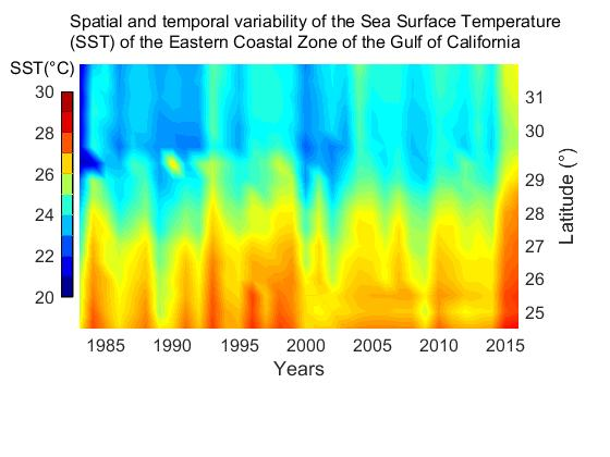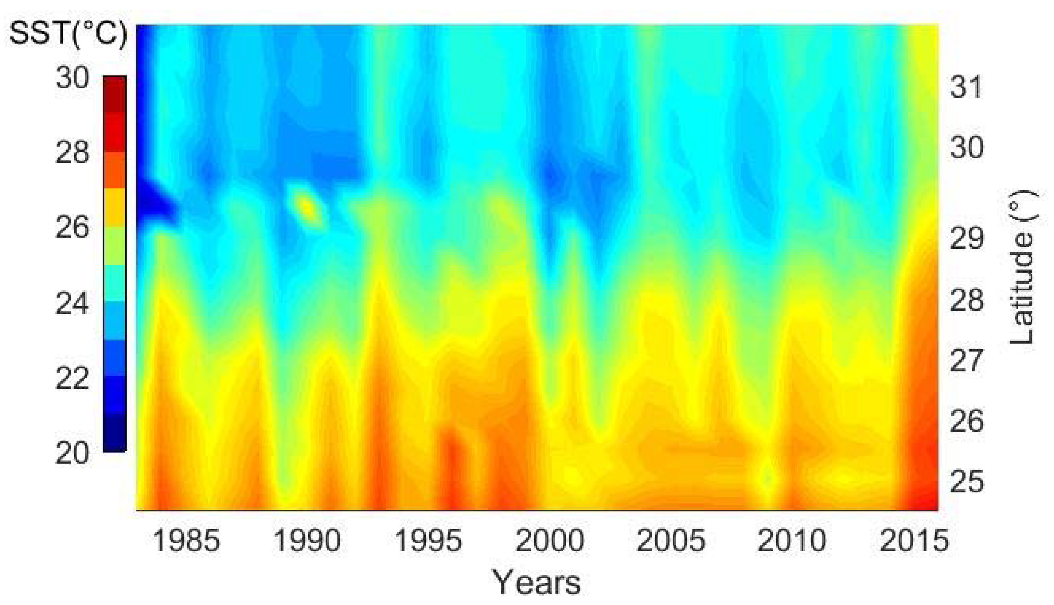The Gulf of California is often cloud free, which makes it ideal for observations using satellite remote sensing techniques [8]. Therefore, the objective of this work is to describe the spatial and temporal variability (regional and monthly) of the SST in the Eastern Coastal Zone of the Gulf of California using a 415-month (September 1981–March 2016) series of remote sensor databases.

2. Materials and Methods

2.1. Study Area

This study comprised the Eastern Coastal Zone of the Gulf of California (from the north of Sinaloa State to the delta of the Colorado River) (Figure 1). This coastal region has a great diversity of costal ecosystems with several important fishing ports like Yavaros, Guaymas and Puerto Peñasco, and highly productive irrigated farmlands are located in the coastal plain; it also has a high fertility induced by coastal upwellings [31]. The central region has a seasonal pattern of biological production, pigment concentration, pigment-rich water is found at northeast side (continental side) during early winter (November to December), and sometime later this water expands to southwestern region (peninsula side). Summer conditions contracts the rich water in the opposite direction, remaining a small rich area in the northeastern central coastal zone [32,33,34]. In the Midriff Islands area, there is a vertical distribution of nutrients constantly associated to tidal mixing [35]. Hidalgo-González et al. [36] indicated near from the Tiburón Island and Ángel de la Guarda Island there are sills and deep basins forming tidal streams developing a particular behavior in the distribution of the temperature with different levels in the south of Ángel de la Guarda and Tiburón Island [37]. We retrieved SST data from 17 georeferenced sites (sampling points), from the Eastern Coast of the Gulf of California. These sampling points were 60 km separated from each other and 30 km from the coastline, that ranges from the northern Sinaloa to northern Sonora (

Table 1. List of geographic coordinates of the sampling points of the Eastern Coastal Zone of the Gulf of California.

Sampling Point	Geographic Coordinates	Sampling Point	Geographic Coordinates	Sampling Point	Geographic Coordinates
1	24°48′N, 108°24′W	8	27°36′N, 111°W	15	30°24′N, 113°18′N
2	25°12′N, 108°54′W	9	28°N, 111°36′W	16	30°48′N, 113°24′W
3	25°36′N, 109°42′W	10	28°24′N, 112°W	17	31°12′N, 113°48′W
4	25°60′N, 109°42′W	11	28°42′N, 112°12′W
5	26°24′N, 109°42′W	12	29°12′N, 112°42′W
6	26°48′N, 110°12′W	13	29°36′N,112°54′W
7	27°12′N, 110°48′W	14	30°N, 113°6′W

).

2.2. Oceanographic Characterization and Obtaining Data of the Sea Surface Temperature (SST)

The SST data were obtained of the Physical Oceanography Distributed Active Archive Center (PODAAC) of the Jet Propulsion Laboratory California Institute of Technology (https://podaac.jpl.nasa.gov/) and OceanColor Web (https://oceancolor.gsfc.nasa.gov/) from NASA, processed at level 3 and downloaded in HDF (Hierarchical Data Format). The data processing from PODAAC at level 3 consist on variables mapped on uniform space-time. The all-pixel SST files contain values for each pixel location, including those contaminated with clouds or other sources of error. The Overall Quality Flag values may be used to filter out these unwanted values. The SST value in each pixel location is an average of the highest quality AVHRR Global Area Coverage (GAC) observations available in each roughly 4 km bin. First-guess SST, the Pathfinder algorithm uses a first guess SST based on the Reynolds Optimally Interpolated SST (OISST), Version 2 product. The OISST V2 is also used in the quality control procedures. That is this parameter indicates the number of AVHRR GAC observations falling in each approximately 4 km bin, as well as standard deviation of the observations in each 4 km bin. Overall Quality Flag, the overall quality flag is a relative assignment of SST quality based on a hierarchical suite of tests. The Quality Flag varies from 0 to 7, with 0 being the lowest quality and 7 the highest. For most applications, using SST observations with quality levels of 4 to 7 is typical, this being the quality indicator that was used to validate the AVHRR GAC images, since the of the pixels of poor values (level 0) are discarded in the first tests of condition, quality or error. For applications requiring only the best-available observations (at the expense of the number of observations), use quality levels of 7 only [39].

The data processing from OceanColor are of geophysical variables that have been projected onto a well-defined spatial grid over a well-defined time period, each file contains an equirectangular projection and a registration of structure square cells grids grid of floating-point values for a single geophysical parameter. NASA standard processing and distribution of the SST products from the MODIS sensors is now performed using software developed by the Ocean Biology Processing Group (OBPG). The OBPG generates Level-2 SST products using the Multi-Sensor Level-1 to Level-2 software (l2gen), which is the same software used to generate MODIS ocean color products. The SST algorithm and quality assessment logic are the responsibility of the MODIS Science Team Leads for SST (currently P. Minnett and R. Evans of the Rosenstiel School of Marine and Atmospheric Science at the University of Miami). The description is valid for both the standard products distributed by the OBPG through the ocean color web and the products delivered to the Physical Oceanography DAAC, where the latter are subsequently repackaged for GHRSST distribution. MODIS Aqua Global Level 3 Mapped Thermal SST products consists of sea surface temperature (SST) data derived from the 11 and 12 um thermal IR infrared (IR) bands (MODIS channels 31 and 32). Daily, weekly (8 day), monthly and annual MODIS SST products are available at both 4.63 and 9.26 km spatial resolution and for both daytime and nighttime passes. This particular dataset is the MODIS Aqua, thermal-IR SST level 3, 4 km, daily, daytime product (ftp://podaac-ftp.jpl.nasa.gov/allData/modis/L3/docs/modis_sst.html).

The sensors used of the PODAAC portal to obtain the SST data were Advanced Very High Resolution Radiometer (AVHRR-Pathfinder Version 5.1) for the period from September 1981 to January 1985 and Advanced Very High Resolution Radiometer (AVHRR-Pathfinder Version 5) for the period from February 1985 to June 2002. These sensors correspond to day period in Celsius degrees (°C) with pixel size 4 × 4 km². However, due the AVHRR-Pathfinder sensor only presents SST data until 2009, the other sensor used was Aqua MODIS Sea Surface Temperature (11µ daytime) in scale of degree centigrade (°C) with a resolution of 4 km from the OceanColor Web for the period from July 2002 to March 2016 with the objective to construct and continue a database of 415 months. This last sensor is of the new generations of radiometers that combine a wider range of spectral measurement with improvements in technology, the values measured with both sensors are similar [40]. The satellite images were processed with the Windows Image Manager (WIM), WimSoft version 9.06 Software (Copyright Mati Kahru 1995–2015) to obtain the SST monthly mean data of the 17 sampling points transect of the coastal zone.

2.3. Analysis and Processing Monthly Data of SST

Before performing the statistical analysis that will be presented here, SST data were previously inter-calibrated to adjust the values from the different sensors used, by means of lineal regression in each one of the data pair where the SST were obtained. This process was developed using a five years’ period where both sensors coincide (July 2002–July 2007), a strong correlation between both data and an intersection that is not significantly different from zero indicated that the values are practically similar. Monthly SST comparisons of different sensors have done to validate the combination of these sensors, obtaining a similar distribution pattern and a high correlation coefficient justifying the analysis of long SST time series from different sensors [40]. Each regression equation (AVHRR-Pathfinder VS Aqua MODIS) was used to adjust the SST data of the Aqua MODIS.

Once the sensor data were inter-calibrated, a cluster analysis was carried out, with the purpose of grouping the sampling points with greater homogeneity among them, and greater difference (statistical distance) between the groups. A nonparametric test (Kruskal-Wallis, p < 0.05) was used to show the statistical differences between the groups obtained from the cluster analysis. A descriptive analysis that includes tables, box plots and Receiver Operating Characteristic (ROC) curves were done to analyze the climatology and time series by regions and during the different months. The ROC curves, is a statistical tool, which are widely used for assessing the performance of classification algorithms. The class assignment is made comparing a score or measurement, with a threshold: If the score is above the threshold, it is assigned to one class, otherwise, is assigned to the other class [41]. In this way, ROC curves allows us to identify if we could differentiate between two regions, based on their mean SST values. On the other hand, a simple way to see if the classifier has the ability to discriminate between two populations or in this case, two regions, is checking if the Area Under the Curve (AUC) is significantly greater than 0.5, the chance diagonal. From an averaged time series of each group, a Fast Fourier Transform was performed to obtain the spectral density. The software Statistical Software version 7.5 and R Software version 3.3.2 performed all the analyzes.

3. Results

3.1. Distribution and General Variability of SST

The overall SST distribution (Figure 2) evince a latitudinal gradient. The warmest SST values were located at the entrance of the gulf, with average values higher than 26 °C, and the coldest SST values from the Midriff Islands to the north, with average values lower than 24 °C.

The coastal zone SST rapidly increases from minimum values of 18 to 20 °C (January and February) to maximum temperatures of 30 to 32 °C (August and September). Two well defined periods were observed in the annual SST pattern for the Eastern Coast of the Gulf of California: Warm period with SST higher than 25 °C, and cold period with SST lower than 25 °C, May–June and November are transitions periods with temperatures around the 25 °C (Figure 3).

3.2. Characterization of Regions

Cluster analysis clearly grouped the SST values in four clusters from 20 linkage distance units (Figure 4). The first group includes from the first to the third sampling point, South Region. The second group, Central Region, comprises from the fourth to the tenth sampling point. The third group is the Midriff Islands Region that covers only the eleventh sampling point, and the fourth group is the North Region that spans from the twelfth to the seventeenth sampling point. These regions will be analyzed from now on (

Table 2. Classification of the Regions of the sampling points of the Eastern Coastal Zone of the Gulf of California.

Sampling Point	Region	Sampling Point	Region	Sampling Point	Region
1	South Region	8	Central Region	15	North Region
2	South Region	9	Central Region	16	North Region
3	South Region	10	Central Region	17	North Region
4	Central Region	11	Midriff Islands Region
5	Central Region	12	North Region
6	Central Region	13	North Region
7	Central Region	14	North Region

).

3.3. Time Series and Climatology

The averaged time series for SST of each group showed values between 12 and 36 °C. The South Region presented the narrowest range, between 17 and 32 °C (Figure 5), while Central Region has a range of values between 16 and 32 °C (Figure 6). On the other hand, Midriff Islands Region (Figure 7) presented the widest range of values (12 to 36 °C) and the North Region (Figure 8) has the similar range as the Central Region.

The SST anomalies varied from −5.5 to 4.3 °C. The South Region has the narrowest range between −2.9 and 2.8 °C (Figure 9) and the Midriff Islands Region showed the widest range of values between −5.5 and 4.3 °C (Figure 10). The Central and North Region anomalies varied from −4.1 to 2.9 °C (Figure 11) and −4.8 and 2.4 °C (Figure 12). The SST anomalies were compared with a database of Southern Oscillation Index (SOI) from the Equatorial Pacific Ocean downloaded from ClimateDateGuide (https://climatedataguide.ucar.edu/climate-data/nino-sst-indices-nino-12-3-34-4-oni-and-tni) with a range between −3.4 and 4.2 indicating that the positive anomalies are associated to El Niño event and a negative anomalies are associated to La Niña event.

Some overall statistics for SST are described in

Table 3. Descriptive statistics of SST for each region of the Eastern Coastal Zone of the Gulf of California.

Region	Mean ± SD (°C)	Maximum (°C)	Minimum (°C)
South	25.81 ± 4.28	32.43	16.76
Central	24.80 ± 4.77	32.41	15.71
Midriff Islands	23.67 ± 5.68	36.30	11.90
North	23.49 ± 5.01	31.83	15.48

. This table contains the mean, standard deviation, as well as the maximum and minimum of SST, for each region, and clearly, we can observe a decrease in the SST mean value from south to north region.

For each of these regions a similar variability was observed, with different time intervals of the transitions periods around 25 °C (Figure 13). The South Region present the transition to summer between April and May reaching maximum values in August and September for seven months of warm period with a mean of 28.53 °C and a maximum of 32.43 °C, while the transition to winter starts between November and December reaching the minimum values in February for five months of cold period with a mean of 22.10 °C and a minimum of 16.76 °C. The Central Region begins its transition to summer between May and June reaching the maximum values in August and September for seven months of warm period with a mean of 28.55 °C and maximum of 32.41 °C, while the transition to winter starts again between November and December obtaining minimum values in January and February for six months of cold period with a mean of 21.12 °C and a minimum of 15.71 °C. The Midriff Islands Region begins the transition to summer between May and June with maximum values in August for five months of warm period with a mean of 28.77 °C and maximum of 36.30 °C, while the transition to winter that starts between October and November with minimum values in January for seven months of cold period with a mean of 20.08 °C and a minimum of 11.90 °C. The North Region has a summer transition that begins in June with maximum values in August for four months of warm period with a mean of 29.01 °C and a maximum of 31.83 °C, while the transition to winter begins between October and November having minimum values in February for eight months with a mean of 20.76 °C and a minimum of 15.48 °C.

According to the statistics for SST during each one of the periods (warm and cold) that are described in

Table 4. Descriptive statistics of SST for each region of the Eastern Coastal Zone of the Gulf of California (warm period).

Region	Time	Mean ± SD (°C)	Maximum (°C)	Minimum (°C)
South	7 Months	28.53 ± 3.00	32.43	19.49
Central	6 Months	28.55 ± 2.96	32.41	18.94
Midriff Islands	5 Months	28.77 ± 3.32	36.30	13.92
North	4 Months	29.01 ± 2.18	31.83	24.03

and

Table 5. Descriptive statistics of SST for each region of the Eastern Coastal Zone of the Gulf of California (cold period).

Region	Time	Mean ± SD (°C)	Maximum (°C)	Minimum (°C)
South	5 Months	22.10 ± 2.68	28.03	16.76
Central	6 Months	21.12 ± 3.06	30.79	15.71
Midriff Islands	7 Months	20.08 ± 3.99	34.85	11.90
North	8 Months	20.76 ± 3.55	29.47	15.48

, the SST gradients are reversed in each period. During the warm period, the months of summer decreased in time from south to north, as well as SST mean values increased from south to north. During the cold period, the months of winter increased in duration and the SST mean values decreased from south to north.

For the comparison of the monthly SST values in the warm and cold period between the four regions, a Kruskal-Wallis test was performed. The monthly SST values of the warm period between these regions were not statistically different (p = 0.7763); however, the monthly SST winter values were statistically different (p < 0.0001). Differences of monthly SST mean of the cold period values were confirmed by a Bonferroni multiple comparison post hoc test. Significant p values (2-Tailed) are denoted with an asterisk in

Table 6. Multiple comparison p values (2-Tailed) of the monthly values of the cold periods with a Bonferroni adjustment of each one of the regions of the Eastern Coastal Zone of the Gulf of California. Asterisk (*) denotes probability values of statistical differences.

	South	Central	Midriff Islands	North
South		0.003880 *	0.000000 *	0.000000 *
Central	0.003880 *		0.000094 *	0.339130
Midriff Islands	0.000000 *	0.000094 *		0.048219 *
North	0.000000 *	0.339130	0.048219 *

, where can be observed that only North and Central Regions are not statistically significant.

A Box-Whisker plot for winter SST mean values can be observed in Figure 14, where a clear difference in variability can be seen. Graphically the differences between the regions obtained in Table 5 were presented using ROC Curves based on the mean SST values. It is clear that during the warm period the South and Midriff Islands Regions are practically similar with a low sensitivity and specificity levels (0.617, 0.462) and a confidence interval for the Area Under the Curve (AUC) of (0.47, 0.584), where 0.5 is into this interval (Figure 15), being not possible to discriminate between these regions. However, during the cold period the results were different obtaining a high sensitivity but low specificity levels (0.943, 0.473) and a confidence interval of (0.656, 0.755) for AUC, obtaining clear differences between these regions (Figure 16).

3.4. Fourier Analyses

The SST spectral analysis of the regions (Figure 17, Figure 18, Figure 19 and Figure 20) showed that the main frequencies are annual associated with maximum levels in summer and minimum levels in winter, semiannual (six months), and also interannual (periods of three to five years), whose frequencies of variation are associated to global climatological-oceanographic phenomena such as El Niño and La Niña. In addition to all these frequencies, also a seasonal variability can be observed in some regions (South, Central and Midriff Islands), but not at the North Region. The spectral analysis showed an increase in the semiannual frequency from the South to the North Region as well an increase in the seasonal frequency in the Midriff Islands Region reaching almost the same semiannual spectral density level. The interannual frequency rise in the Midriff Islands Region, as well, a possible rise of the decadal frequency.

4. Discussion

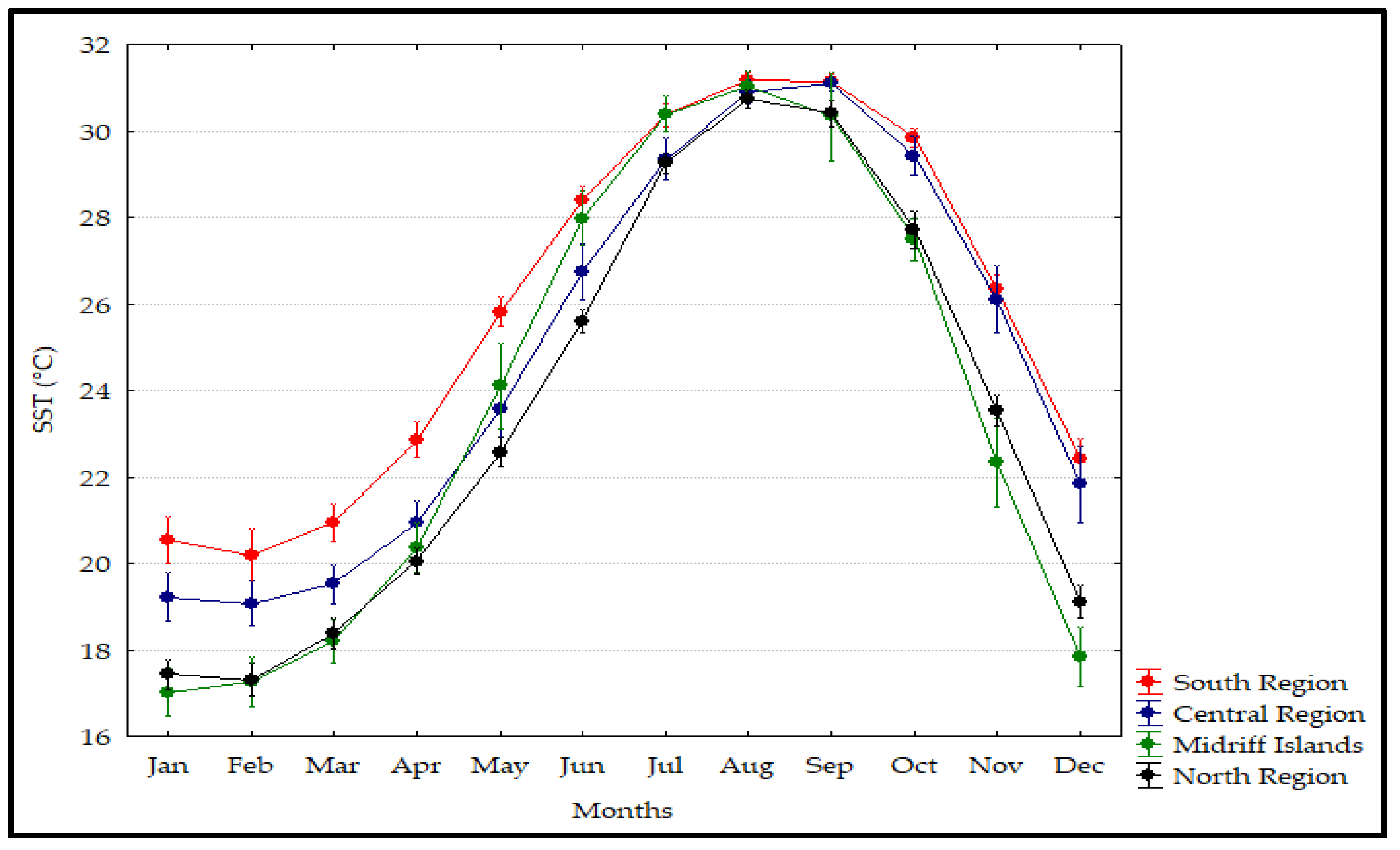
The SST during the year is similar to the values reported by Robles and Marinone [25] and Valenzuela-Sánchez [23] allowing establishing a general climatology, highlighting the occurrence of two clearly defined periods. A warm and a cold period, with very short transition periods. The climatology of the Gulf of California has been described by Roden [42], showing clear latitudinal differences and from the east and west coasts, related to atmospheric circulation and mountain ranges that influences its circulation. The SST mean values of the study area decreased from south to north during the warm period, and reversed during the cold period. This gradient from south to north is similar to the results for whole Gulf of California described by Soto-Mardones et al. [22], Escalante et al. [24] and Hidalgo-González and Álvarez-Borrego [43]. This SST distribution, during the warm period, can be explained by the fact that the direct communication with the Tropical Pacific Ocean allows the entry of Equatorial Surface Water [29,44], and inside the Gulf of California it is modified by greater solar irradiance and evaporation effects [42], generating this gradient. 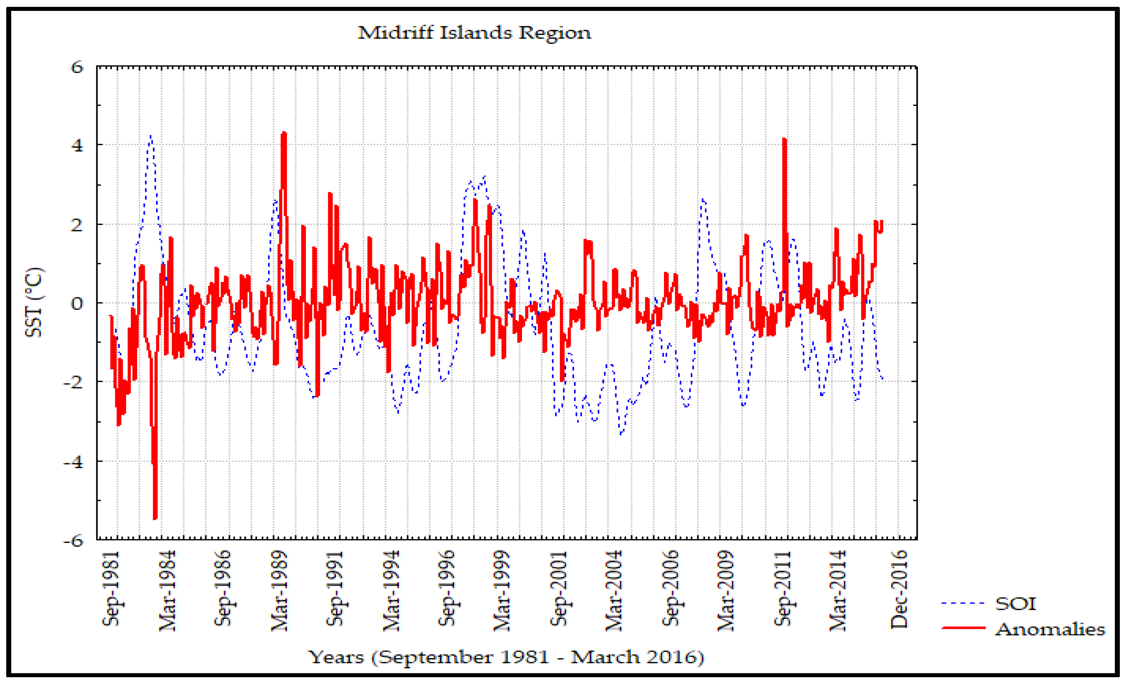During the cold period, SST decrease inside the Gulf by physical dynamics such tidal and wins mixing [25], mainly in the Midriff Islands and North Regions. In addition, the effect of the continental meteorological conditions in the northern Gulf of California are important in the decrease of the SST [42,45]. Low temperatures are found all around the year in the Midriff Islands, where winds and tides [46], hydraulic jump [8] and strong currents through the narrow channels mix the water column. López et al. [47] reported a decrease on SST in this region, coldest SST were associated to tidal pumping and mean flow in the sills in the southern part of this region, developing a particular circulation pattern that generates persistent upwelling of deep waters causing low SST values, high productivity and well mixed conditions throughout the water column. A more constant SST at the entrance of the Gulf allows these gradients to exist, as well as, the varying duration of warm or cold periods. The further south the duration of the warm period is longer, and the cold period is shorter.

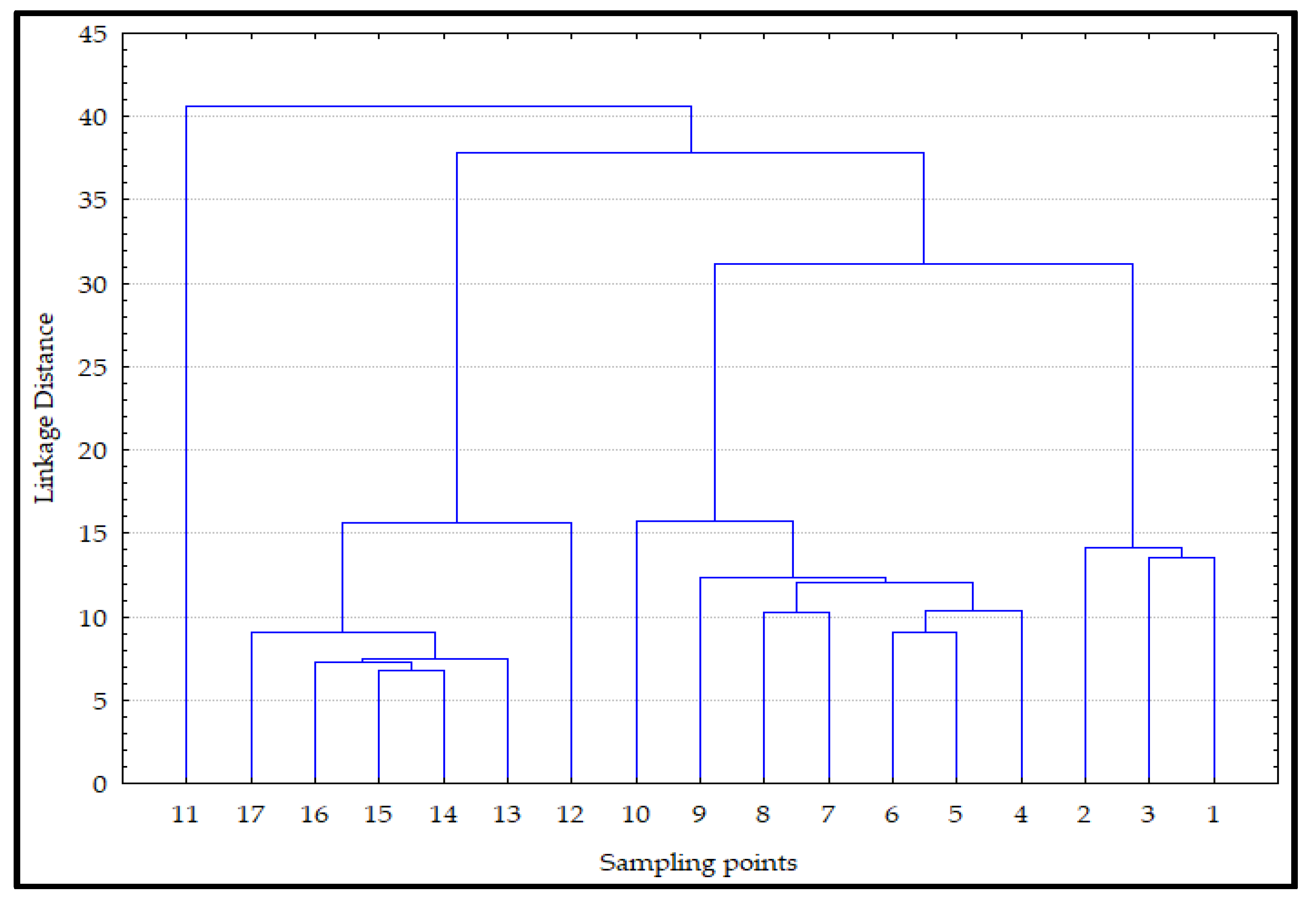
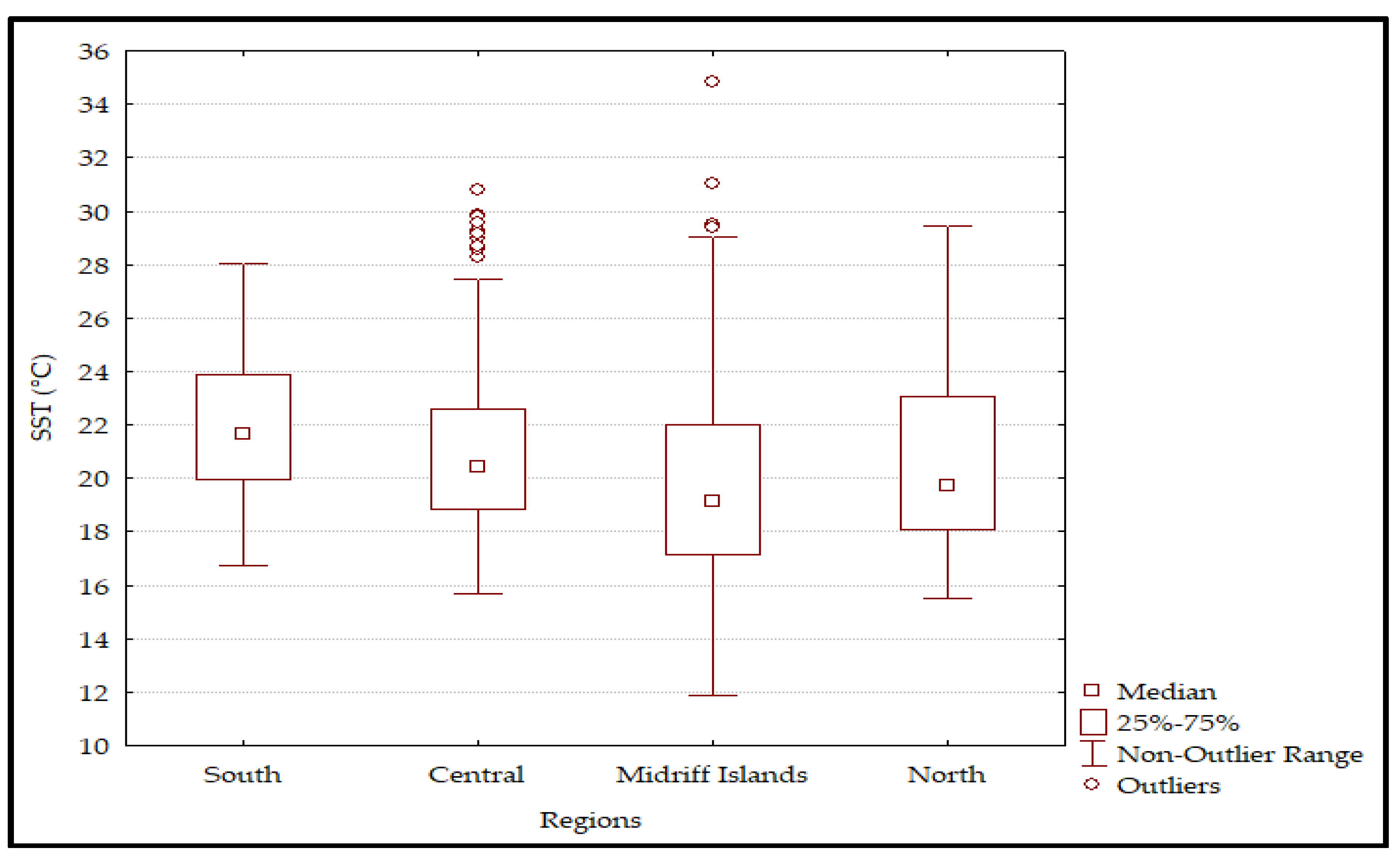
Based on the Cluster analysis, four regions were obtained: South, Central, Midriff Islands and North. Different regionalizations have made for the whole Gulf based on different aspects: Round [48] on the phytoplankton remains in sediments. Santamaría-del-Angel et al. [6] used a time series of Chl a in a number of stations throughout the gulf and for a short period (eight years). Hidalgo-González and Álvarez-Borrego [43] analyzed Chl a data during the cold season along the Gulf of California and Heras-Sánchez [30] used a combination of SST and Chl a for a period of 18 years included in their regionalizations the coastal zone of the Gulf. Our results agree with Hidalgo-González and Álvarez-Borrego [43], and also are very similar with Heras-Sánchez [30], who identified four regions of the Gulf of California with three trophic levels with a clear seasonality. The results of this work are different from Santamaría-del-Angel et al. [6], because they obtained 14 regions using eight years chlorophyll weekly composites of the Coastal Zone Color Scanner data. The high chlorophyll variability associated to physical phenomena such as the movement of water masses and the upwelling systems generated a greater number of regions along the Gulf of California.

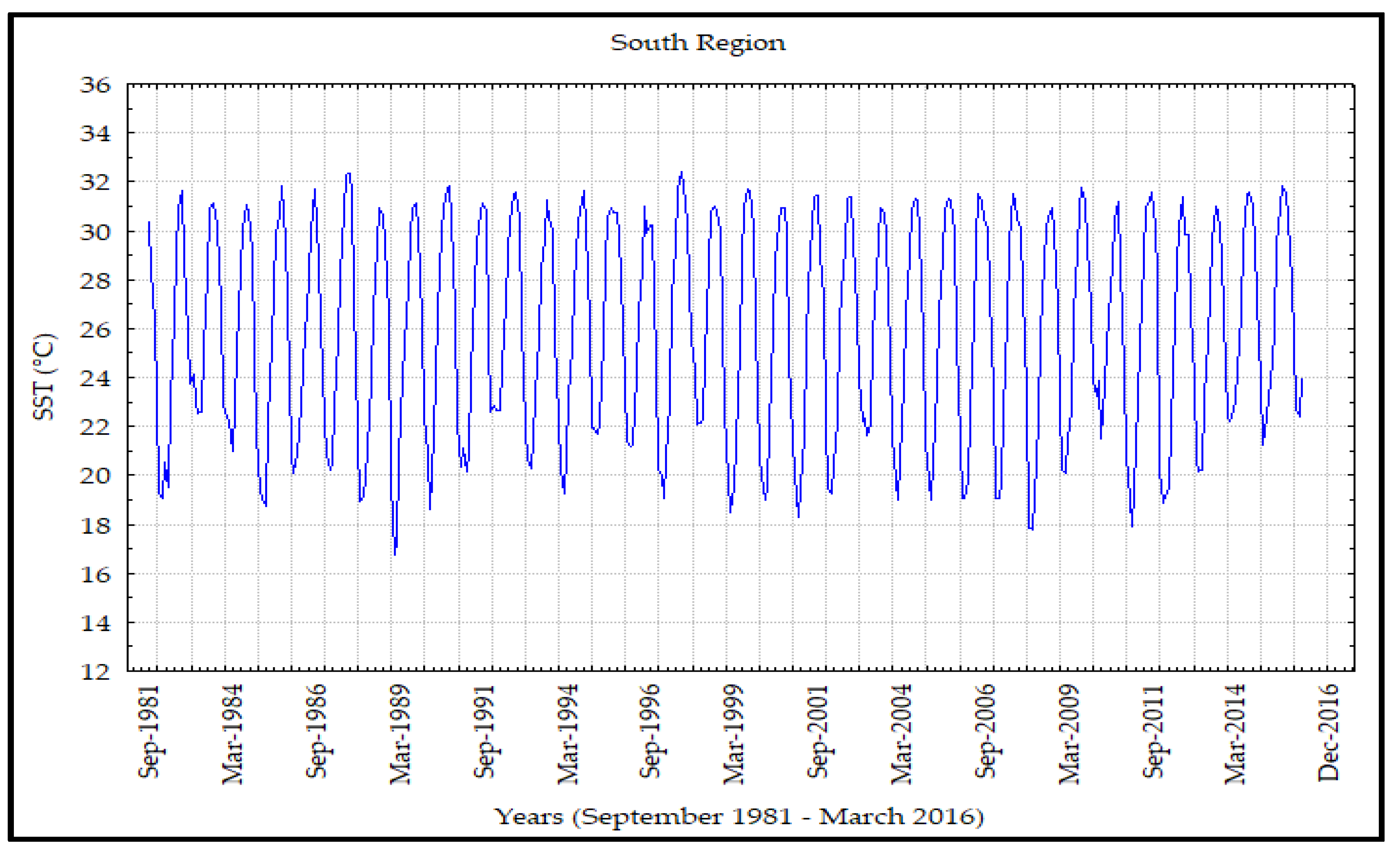
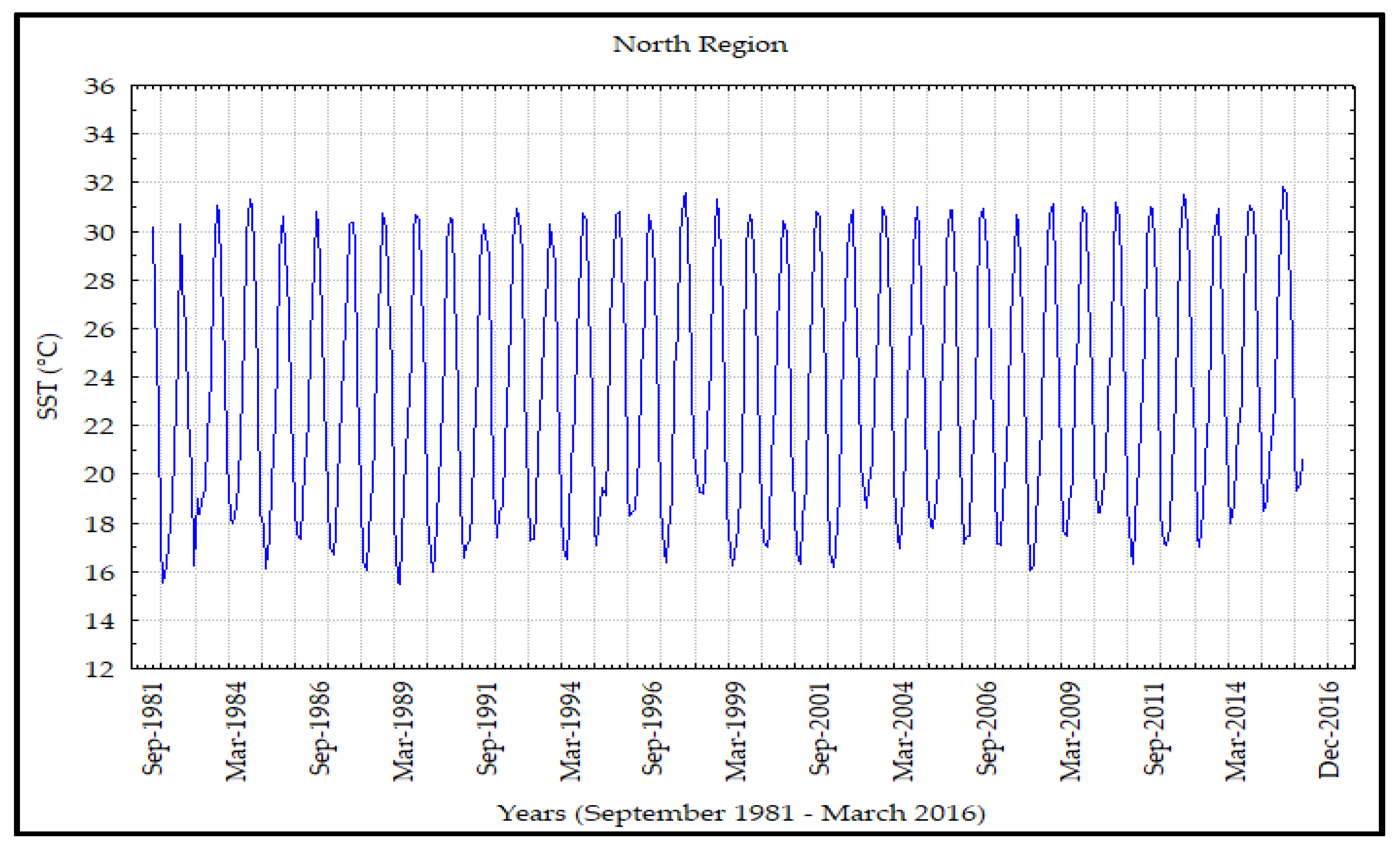
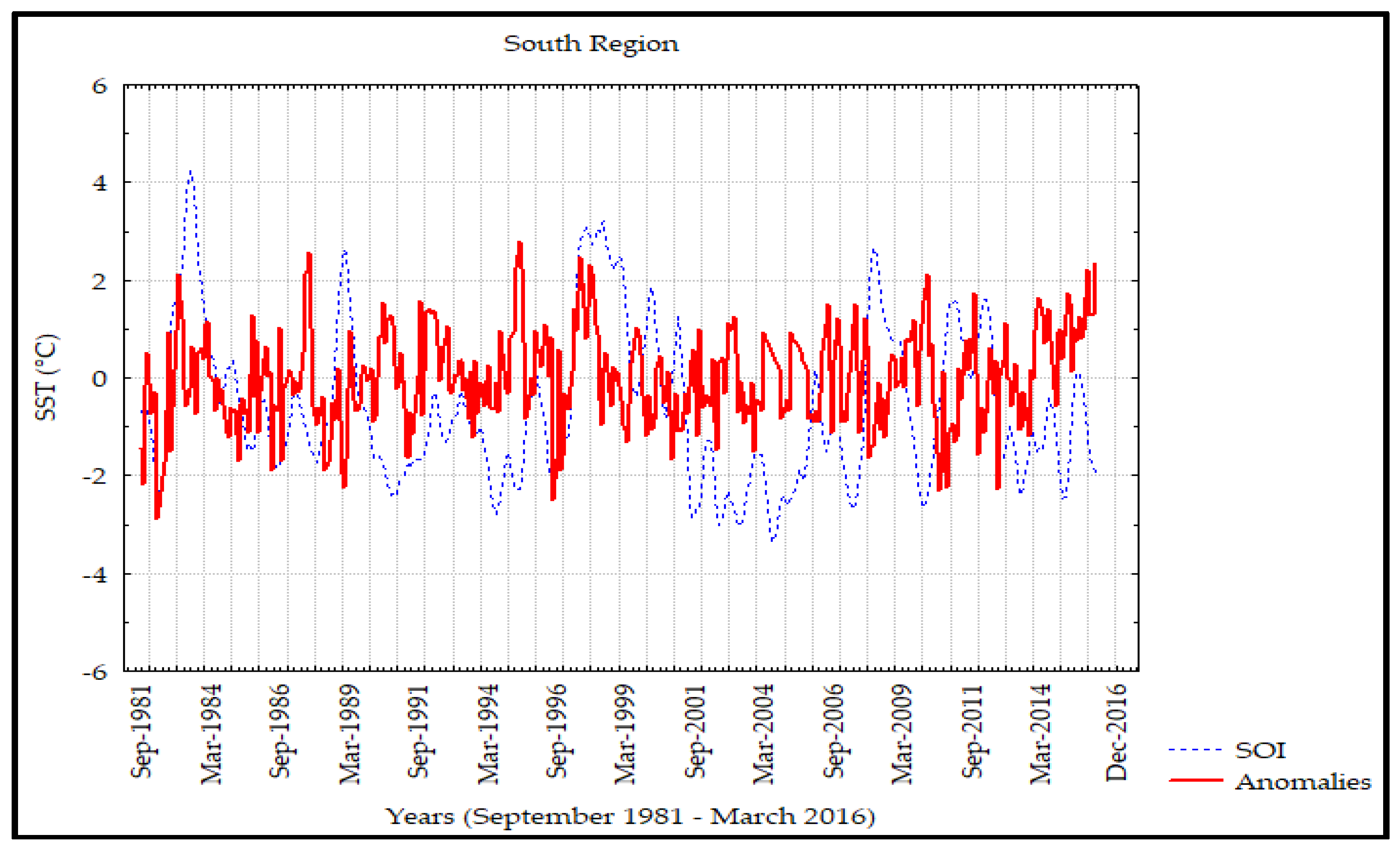
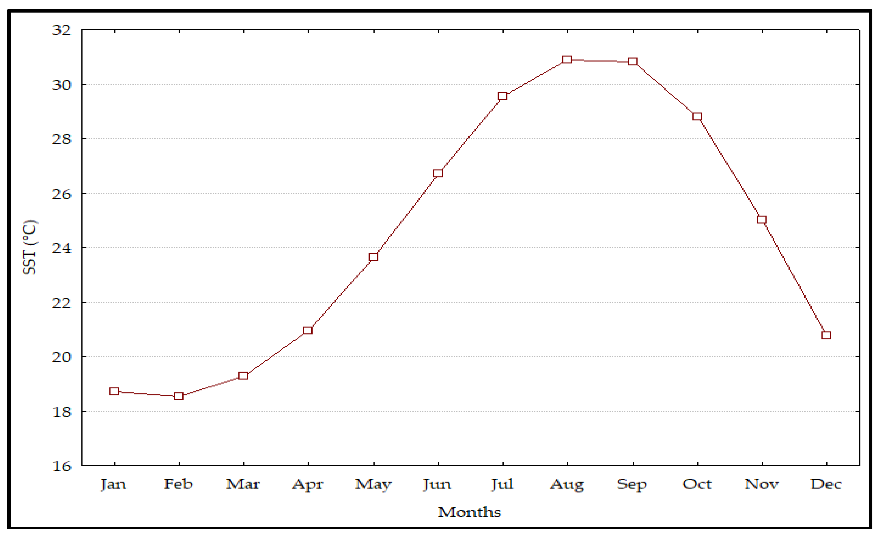
The South Region is directly influenced by the tropical Pacific, and has a more homogenous temperature distribution throughout the year. During the summer with the northward displacement of the Inter-Tropical Convergence Zone (ITCZ) [27], there is advection of water of tropical origin. The SST climatology of this region, maximum values during August and September and minimum during January and February, agreed with the observed by Castro et al. [49] at the entrance of the Gulf of California, showing a seasonal increase of the thermocline, due to the exchanges that take place when alternating the inflow and outflow of water masses. These conditions reported by Castro et al. 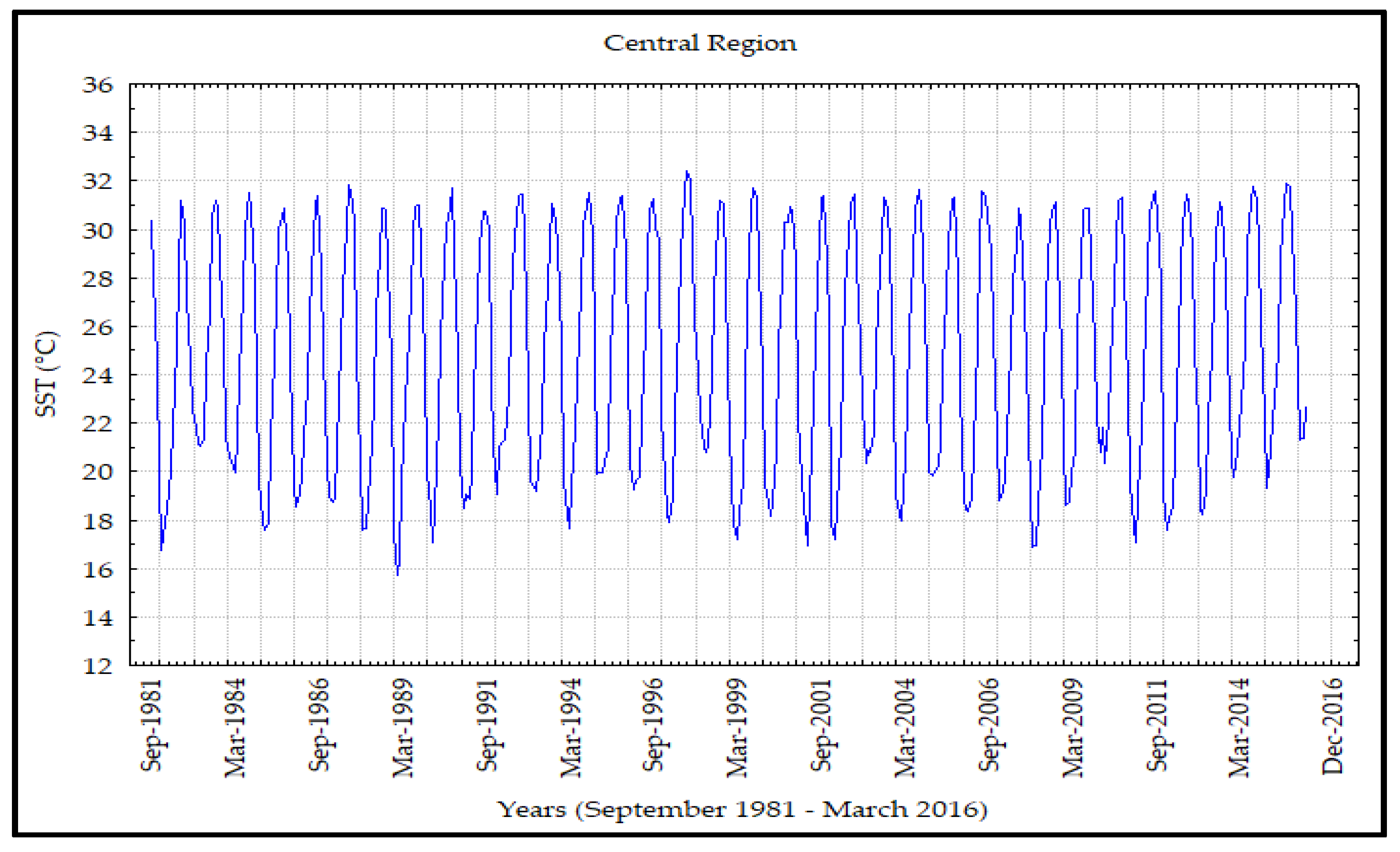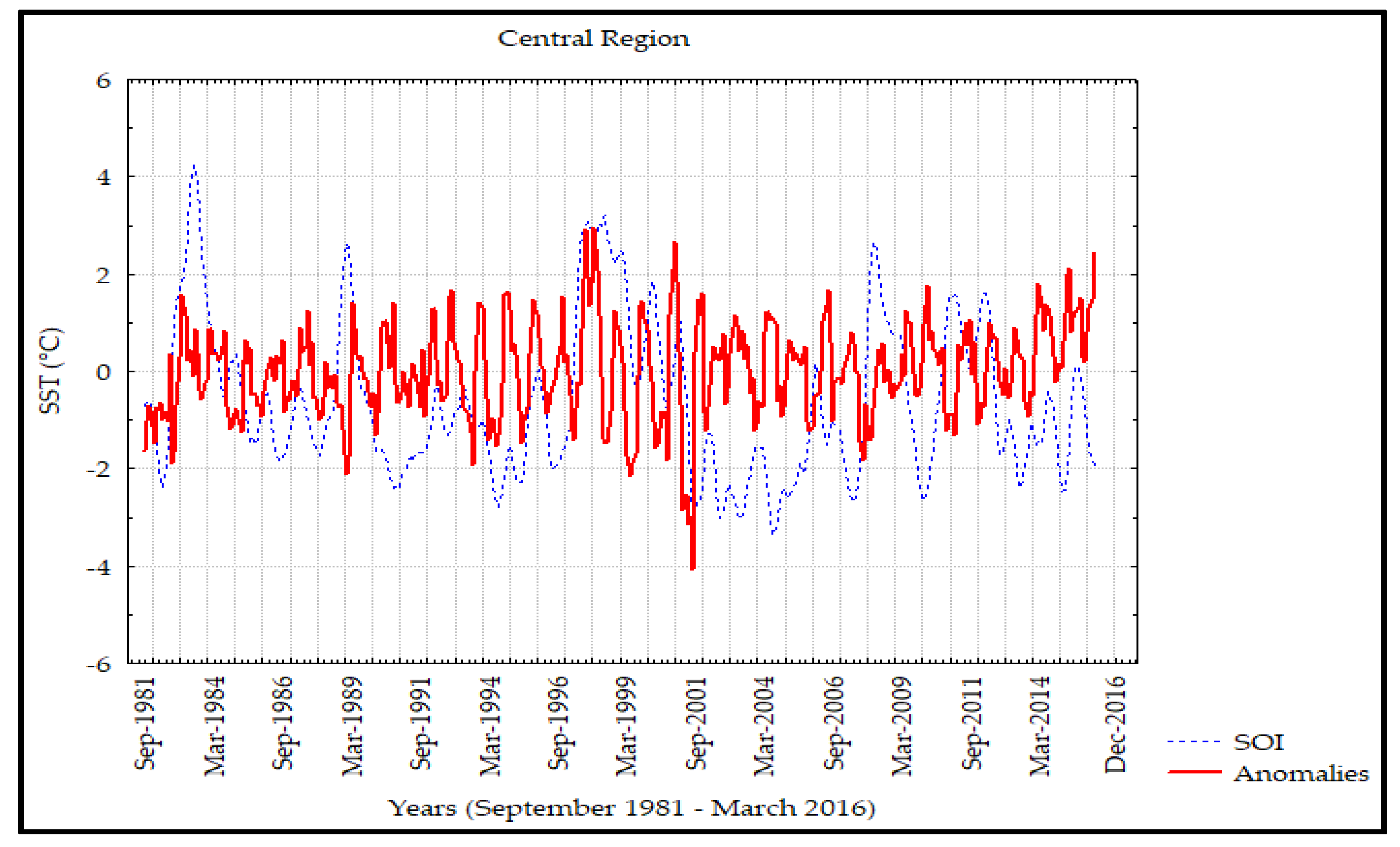[49] can extend to the Central Region, and agree with the one reported by Robles and Marinone [25] in the Guaymas Basin. They found winter conditions from December to April and summer conditions from June to October, with an increase of SST from 16° in February–March to 31 °C in August. The SST values were similar to Valenzuela-Sánchez [23], Soto-Mardones et al. [22] and García-Morales et al. [29], as well as in this study. Bernal et al. [50] report that the variability in this region is caused by the effects of seasonal winds and the oceanographic influence from the Pacific Ocean, the seasonal coastal winds develop a sea surface circulation along the Eastern Coast, to the south during October–March and to the north during June–September [8]. 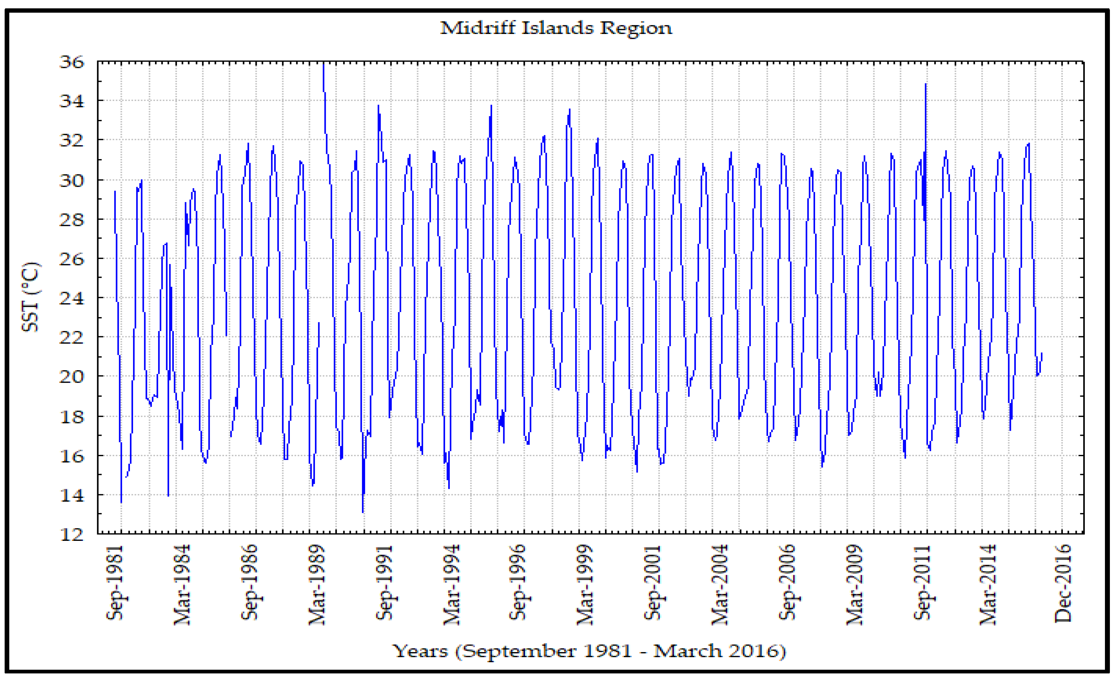Robles and Marinone [25] suggested an advection process of the California Current Water and indicated that Subtropical Subsurface Water may occur around the year in this region, but vertical mixing during winter attenuated their characteristics. Midriff Islands and North Regions presented the lowest minimum in comparison with the ones observed in Central and South Regions. This minimum value is due to the mixing processes in the Midriff Islands Region, system of fronts influenced by seasonal winds and the development of coastal upwellings in the Eastern Coast [8]. Strong currents take place at the channels between the islands, particularly at the Sonora Coast, El Infiernillo Channel is a narrow and shallow channel between Tiburon Island and mainland that allows a well-mixed water column. The North Region is considered a shallow area [4,22], and subjected to a strong tidal mixing in a vertical form as well by the effect of the gravity currents [51] that modulate the distribution pattern of the temperature, the lowest averaged SST observed. However, the maximum temperature values associated with the summer months cause the climatology between each of the regions to cover the same range of values, indicating little difference between them, probably due to the stratification effect, causing the surface temperature of the sea to be constant in each of the regions. In this region, the influence of the continental climate, surrounded by desert with high solar irradiance may be part important of higher temperatures during warm periods.

The range of average annual values was very wide, and almost of the same magnitude, in all the regions of the Eastern Coast of the Gulf. In such a way, the main frequency of variation in each of the regions was the annual, same frequency that was observed by Garcia-Morales et al. [29], Lavín et al. [28] and Herrera-Cervantes et al. [52]. Soto-Mardones et al. [22] showed that the annual scale determines most of the SST variability with small variations from south to north and a warming and cooling process in the entire gulf. The annual variability in the gulf is determined by the influence of the Tropical Pacific Ocean, through the displacement of the Inter-Tropical Converge Zone (ITCZ) that develops latitudinal displacements of all the current systems and consequently modulating the SST values at a seasonal scale [38,53] as well by the influence of the continental climate [42,45]. In addition, the semiannual variability was observed in the four regions. Soto-Mardones [22] showed an increase of the semianual and annual amplitude to the north, with a maximum in the Islands Region. The winds in the gulf are strong and dominant from the northwest (NW) in winter-spring, and weak in summer–autumn with a main component of the southeast (SE) [42,45], upwelling is present in the Eastern Coast during the cold period, while in the warm period the Eastern Coast presents a strong stratification [22,45], with a great semiannual variability in SST. Furthermore, associated to this, winds, surface circulation changes from warm (coastal circulation to the north) to cold (coastal circulation to the south) periods [8]. In the region of the islands, this effect is more important because in this region other physical processes increase semiannual variability: Tide mixing and water and heat flows between the north and central gulf [4,38]. The seasonal cycle is present in these regions, except in the Northern Region, where it is clear that they dominate the annual and semiannual signal, possibly due to a greater influence of the continental desert climate. 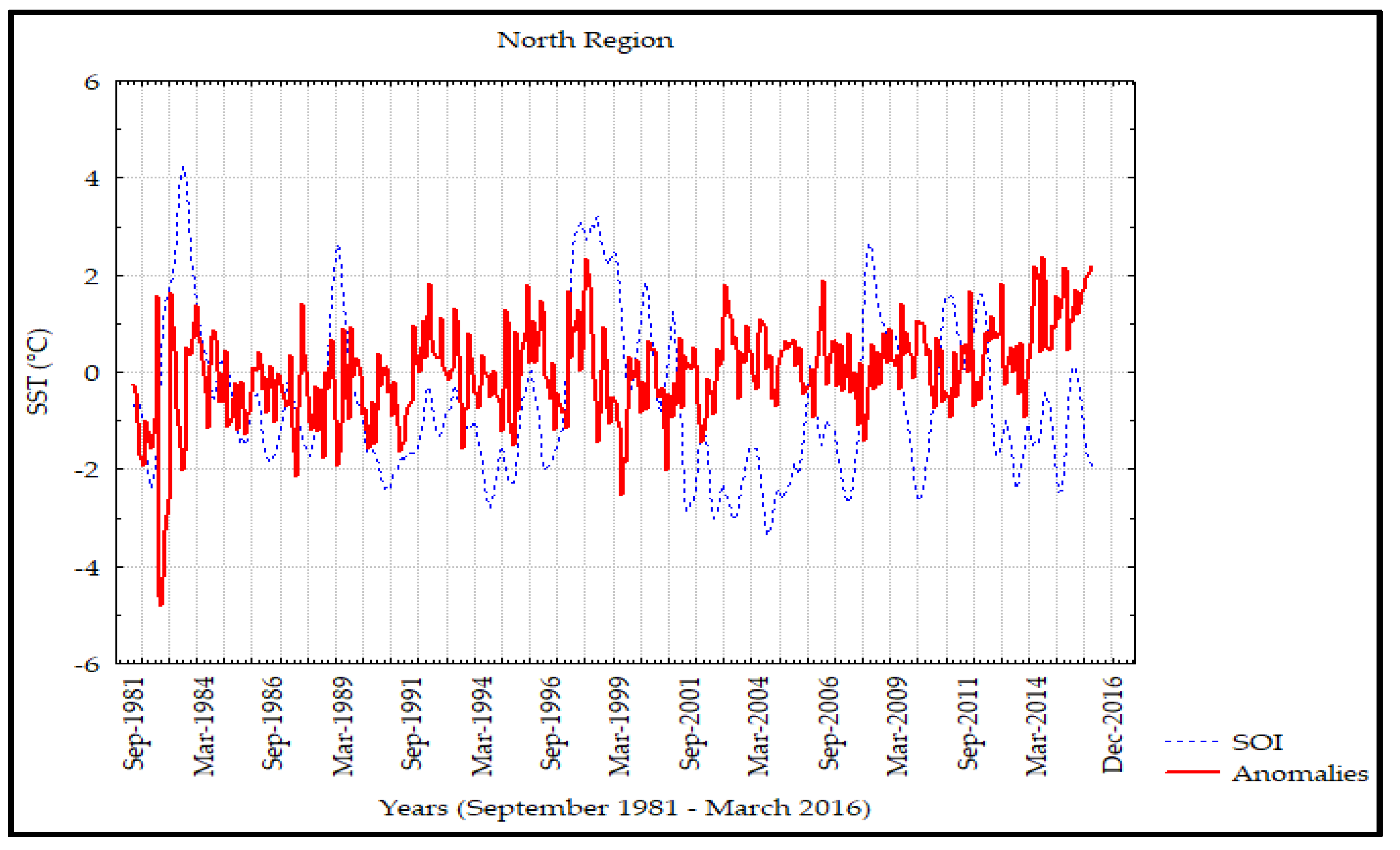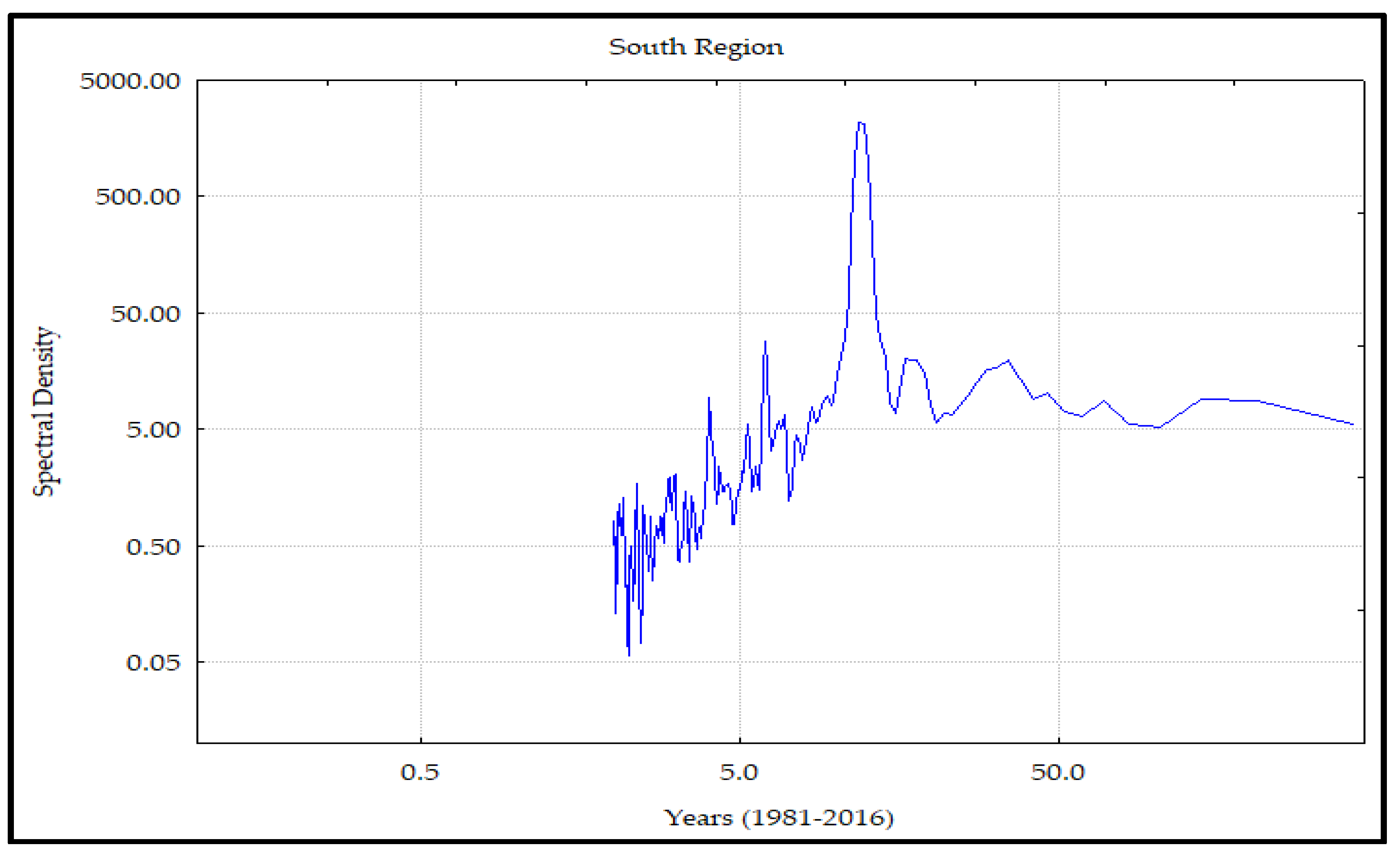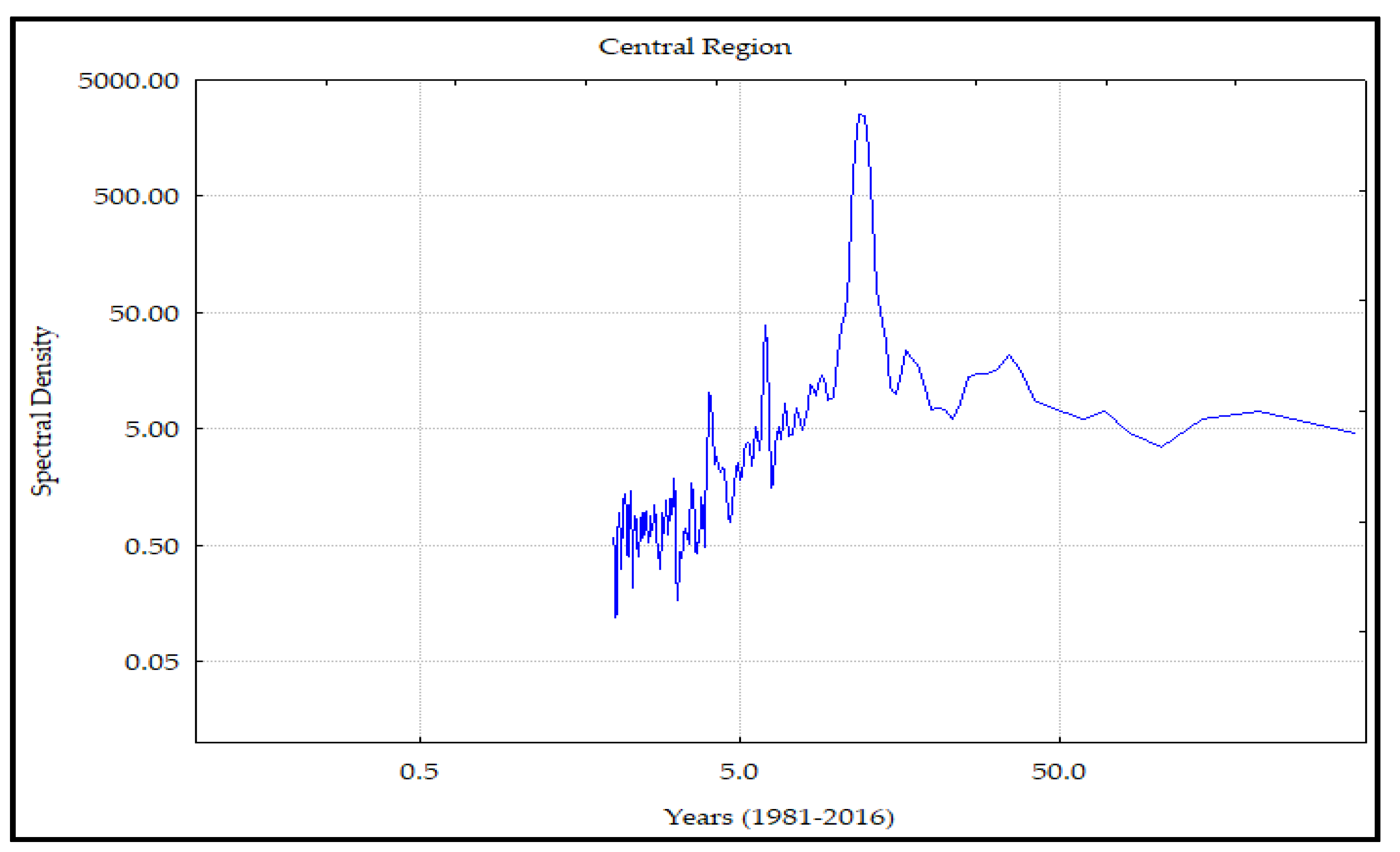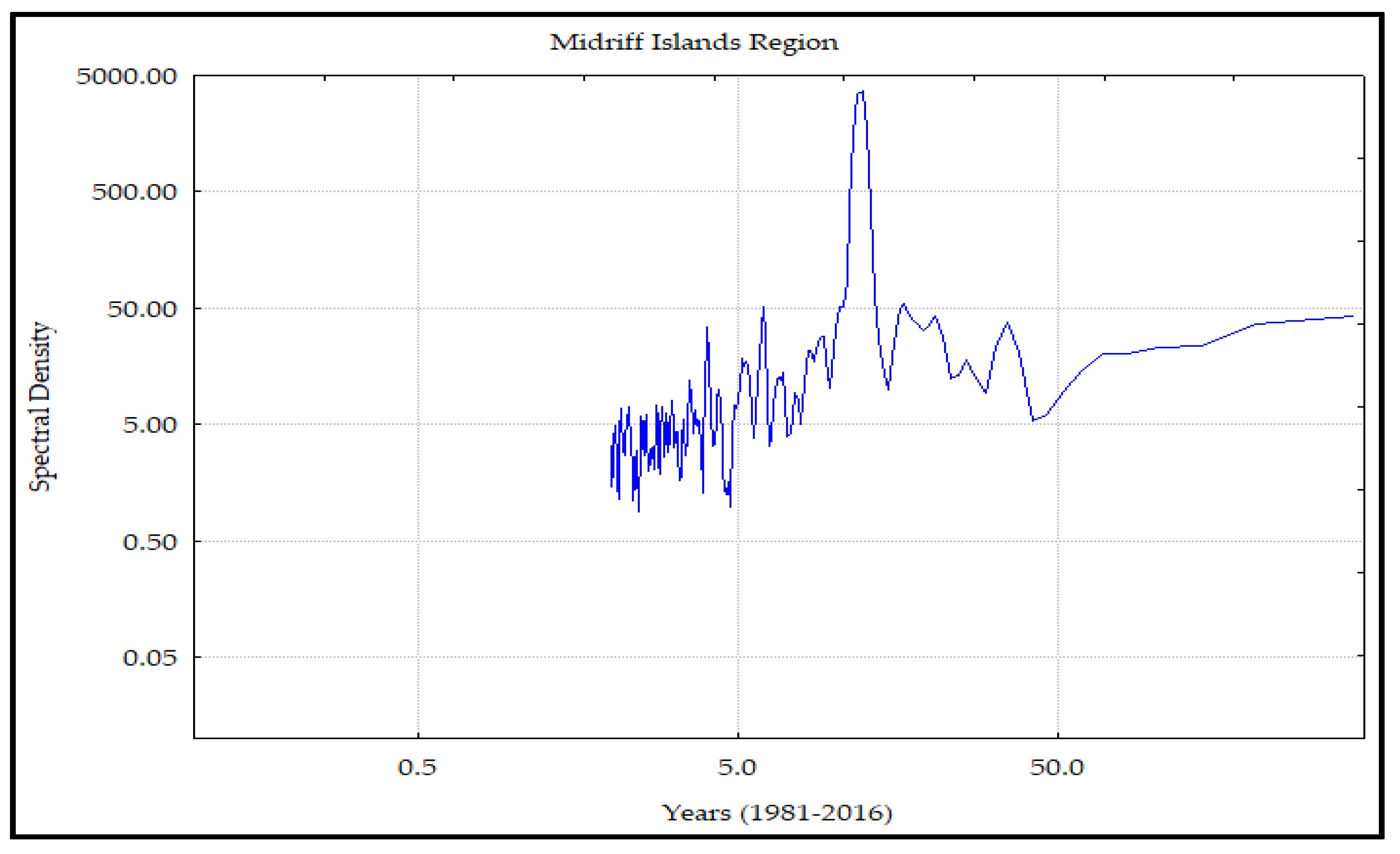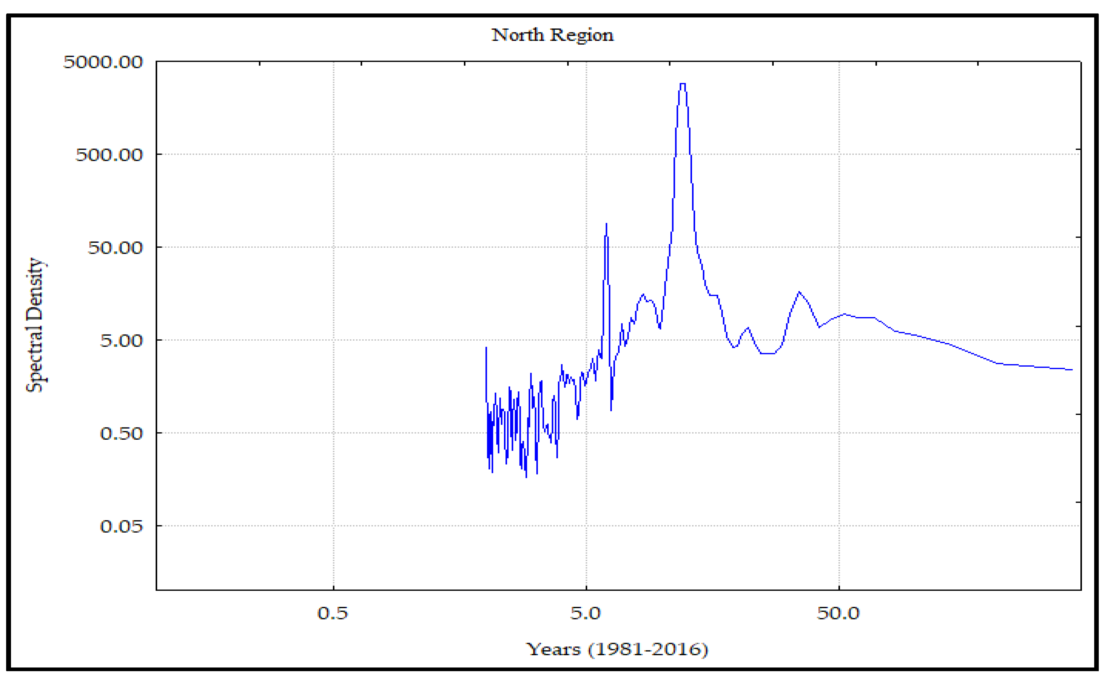Ripa and Marinone [26] indicated a significant seasonal cycle associated to the interaction with the atmosphere through turbulent diffusion of heat, as well horizontal physical processes that contribute in the heat balance in the upper layers. A five-year signal was detected in each of the regions of the coastal zone, this interannual variability is associated with periods such as the El Niño Southern Oscillation. This signal increases from south to Midriff Islands, and then decreased to northern region, the influence of these processes (El Niño–La Niña) in the Gulf have been described by Baumgartner and Christensen [27], Robles and Marinone [25] and Lavín et al. [28]. Lavin et al. [28] explained that the positive anomalies are related to warm water advection of El Niño and negative anomalies associated to La Niña events, with positive anomalies larges in the Central Gulf and the negatives did not have a pattern. Robles and Marinone [25] mention that this signal is attenuated in the central region by mixing processes in this place; in this work, this signal is greater in the region of the Midriff Islands and present in the northern region, according to Herrera-Cervantes et al. [52] concludes that it can be observed in the northern region. Although the spectral analysis requires repeating 10 times the observations of a particular period, it is evident in the region of the islands a variability associated with decadal changes; in the other regions, it is not observed. This frequency of variability, as well as a greater variability in interannual scales, El Niño-La Niña, suggests that the region of the islands is potentially more susceptible to long period events.

The SST variability analysis indicated that this variable is determined mainly by physical and climatological processes in different timescales, with an influence in the coastal ecosystems either a positive or negative effect and consequently to the distribution of the organism. García-Morales et al. [29] found indicating that the SST and chlorophyll a (Chl a) in the central coastal zone of Sonora can influence on the pelagic ecosystems providing productive and biologically rich habitats of diverse species, some of them of commercial interest reported this effect. Nevárez-Martínez et al. [54] obtained similar results when analyzing the distribution and abundance of the Pacific sardine (Sardinops sagax) in the Gulf of California, and its relationship with the environment, determining that the distribution is influenced by the SST and winds that causes upwelling effects. On the other hand, García-Morales et al. [55] determined the influence of environmental variability in the distribution of whales in the Gulf of California, based on the SST and Chl a, they obtained that the largest number of whales were during the cold season of the Gulf of California and the lowest number during the warm season, concluding that the SST influence the relative abundance of the whales while the concentration of Chl a influences its distribution.

5. Conclusions

There is an increase (decrease) of SST mean value from south to north region during the warm (cold) period, with different duration in time and effects in the SST mean values.

A clear semiannual variability in the SST climatology was observed with maximum values in August and September while the minimum values were during January and February. Ranges of the transition periods during summer and winter were different.

Statistical analysis showed that the Eastern Coastal Zone of the Gulf of California can be grouped in four regions. During cold period mean monthly SST values were significant different, something that is not observed during warm period due to homogenization process in the water column.

Based on the results in this research, the four regions of the coastal zone of Sonora have different climatology and transitions periods.

In each one of the regions, the annual variability was the main frequency of variability followed by the variability associated with semiannual, seasonal and interannual events.

The SST analysis showed that the variability is determined by physical and climatological and processes that present different timescales, developing an influence in oceanographic processes as well as in environmental conditions of the coastal zone of Sonora.

References

1. Yañez-Arancibia, A.; Day, J.W. La Zona Costera frente al cambio climático: Vulnerabilidad de un sistema biocomplejo e implicaciones en el manejo costero. In Impactos del Cambio Climático Sobre la Zona Costera, 1st ed.; Yañez-Arancibia, A., Ed.; Instituto Nacional de Ecología (INE-SEMARNAT): México D.F.; Instituto de Ecología A.C. (INECOL): Xalapa, Veracruz, México; Texas Sea Grant College Program: College Station, TX, USA, 2010; pp. 12–35. ISBN 978 607-7579-17-5. [Google Scholar]
2. Hernández-Ayón, J.M.; Camacho-Ibar, V.F.; Mejía-Trejo, A.; Cabello-Pasini, A. Variabilidad del CO2 total durante eventos de surgencia en Bahía San Quintín, Baja California, México. In Carbono en Ecosistemas Acuáticos, 1st ed.; Hernández-de la Torre, B., Gaxiola-Castro, G., Eds.; Instituto Nacional de Ecología, SEMARNAT: México D.F.; Centro de Investigación Científica y de Educación Superior de Ensenada, CICESE: Ensenada, Baja California, México, 2007; pp. 187–200. ISBN 978-968-817-855-3. [Google Scholar]
3. Martínez-López, A.; Cervantes-Duarte, R.; Reyes-Salinas, A.; Valdez-Holguín, J.E. Cambio estacional de clorofila a en la Bahía de La Paz, Baja California Sur. Hidrobiológica 2001, 11, 45–52. [Google Scholar]
4. Lavín, M.F.; Marinone, S.G. An overview of the physical oceanography of the Gulf of California. In Nonlinear Processes in Geophysical Fluid Dynamics, 1st ed.; Velasco-Fuentes, O.U., Sheinbaum, J., Ochoa-de la Torre, J.L., Eds.; Kluwer Academic Publishers: Dordrecht, The Netherlands, 2003; pp. 173–204. ISBN 978-94-010-0074-1. [Google Scholar]
5. Álvarez-Borrego, S. Flujos de carbono en los Golfos de California y México. In Carbono en Ecosistemas Acuáticos, 1st ed.; Hernández-de la Torre, B., Gaxiola-Castro, G., Eds.; Instituto Nacional de Ecología, SEMARNAT: México D.F.; Centro de Investigación Científica y de Educación Superior de Ensenada, CICESE: Ensenada, Baja California, México, 2007; pp. 337–353. ISBN 978-968-817-855-3. [Google Scholar]
6. Santamaría-del-Angel, E.; Álvarez-Borrego, S.; Muller-Karger, F.E. Gulf of California biogeographic regions based on coastal zone color scanner imagery. J. Geophys. Res. 1994, 99, 7411–7421. [Google Scholar] [CrossRef]
7. Álvarez-Borrego, S. Physical, chemical and biological oceanography of the Gulf of California. In The Gulf of California: Biodiversity and Conservation, 2nd ed.; Brusca, R., Ed.; The University of Arizona Press: Tucson, AZ, USA, 2010; pp. 24–48. ISBN 978-0816500109. [Google Scholar]
8. Badan-Dangon, A.; Koblisnksy, C.J.; Baumgartner, T. Spring and summer in the Gulf of California: Observations of surface thermal patterns. Oceanol. Acta 1985, 8, 13–22. [Google Scholar]
9. Álvarez-Arellano, A.D.; Gaitán-Moran, J. Lagunas costeras y el Litoral Mexicano: Geología. In Lagunas Costeras y el Litoral Mexicano, 1st ed.; de la Lanza-Espino, G., Cáceres-Martínez, C., Eds.; Universidad Autónoma de Baja California Sur: La Paz, Baja California Sur, México, 1994; pp. 13–74. ISBN 968-896-048-9. [Google Scholar]
10. Reyes, A.C.; Lavín, M.F. Effects of the autumn–winter meteorology upon the surface heat lost in the Northern Gulf of California. Atmósfera 1997, 10, 101–123. [Google Scholar]
11. Ocean Observations Panel for Climate (OOPC). EOV Spec Sheet: Sea Surface Temperature, Global Ocean Observations System (GOOS) Panel for Physics, EOV-SeaSurfaceTemperature v5.2. Available online: http://goosocean.org/index.php?option=com_oe&task=viewDocumentRecord&docID=17466 (accessed on 8 August 2018).
12. Filipponi, F.; Valentini, E.; Taramelli, A. Sea Surface Temperature changes analysis, an Essential Climate Variable for Ecosystems Service Provisioning. In Proceedings of the 2017 9th International Workshop of Multitemporal Remote Sensing Images (MultiTemp2017), Brugge, Belgium, 27–29 June 2017; Institute of Electrical and Electronic Engineers (IEEE): New York, NY, USA, 2017; pp. 244–251. [Google Scholar]
13. Rojas-Acuña, J.; Eche-Llenque, J.C. La temperatura de la superficie del mar peruano a partir de imágenes AVHRR/NOOA (2000–2003). Rev. Investig. Fis. 2006, 9, 24–30. [Google Scholar]
14. Harley, C.D.G.; Hughes, A.R.; Hultgren, K.M.; Miner, B.G.; Sorte, C.J.B.; Thornber, C.S.; Rodríguez, L.F.; Tomanek, L.; Williams, S.L. The impacts of climate change in coastal marine ecosystems. Ecol. Lett. 2006, 9, 228–241. [Google Scholar] [CrossRef] [PubMed]
15. Doney, S.C.; Ruckelshaus, M.; Duffy, J.E.; Barry, J.P.; Chan, F.; English, C.A.; Galindo, H.M.; Grebmeier, J.M.; Hollowed, A.W.; Knowlton, N.; et al. Climate change impacts on marine ecosystems. Annu. Rev. Mar. Sci. 2012, 4, 11–37. [Google Scholar] [CrossRef] [PubMed] [Green Version]
16. Brierley, A.S.; Kingsford, M.J. Impacts of climate change on marine organisms and ecosystems. Curr. Biol. 2009, 19, 602–614. [Google Scholar] [CrossRef] [PubMed]
17. Morales-Hernández, J.C.; Carrillo-González, F.M.; Farfán-Molina, L.M.; Cornejo-López, V.M. Cambio de cobertura vegetal en la región de Bahía de Banderas, México. Rev. Colomb. Biotecnol. 2016, 18, 17–29. [Google Scholar] [CrossRef]
18. Longhurst, A.R. Ecological Geography of the Sea, 2nd ed.; Elsevier Academic Press: San Diego, CA, USA, 2007; p. 5. ISBN 978-0-12-455521-1. [Google Scholar]
19. Gentemann, C. Three way validation of MODIS and AMRS-E sea surface temperatures. J. Geophys. Res. 2014, 119, 2583–2598. [Google Scholar] [CrossRef]
20. Klemas, V. Remote Sensing Techniques for studying Coastal Ecosystems: An Overview. J. Coast. Res. 2011, 27, 2–17. [Google Scholar] [CrossRef]
21. Rajeesh, R.; Dwarakish, G.S. Satellite oceanography-A review. Aquat. Procedia 2015, 4, 165–172. [Google Scholar] [CrossRef]
22. Soto-Mardones, L.; Marinone, S.G.; Parés-Sierra, A. Variabilidad espaciotemporal de la temperatura superficial del mar en el Golfo de California. Cienc. Mar. 1999, 25, 1–30. [Google Scholar] [CrossRef]
23. Valenzuela-Sánchez, C.G. Tendencia de la Temperatura Superficial del Mar, Nivel Medio del Mar e Incidencia de Vientos en la Región Central del Golfo de California. Master’s Thesis, Maestría en Biociencias de la Universidad de Sonora, Hermosillo, Sonora, México, 25 August 2016. [Google Scholar]
24. Escalante, F.; Valdez-Holguín, J.E.; Álvarez-Borrego, S.; Lara-Lara, J.R. Variación temporal y espacial de la temperatura superficial del mar, clorofila a y productividad primaria en el Golfo de California. Cienc. Mar. 2013, 39, 203–215. [Google Scholar] [CrossRef]
25. Robles, J.M.; Marinone, S.G. Seasonal and interannual Thermohaline variability in the Guaymas Basing in the Gulf of California. Cont. Shelf Res. 1987, 7, 715–733. [Google Scholar] [CrossRef]
26. Ripa, P.; Marinone, S.G. Seasonal variability of temperature, salinity, velocity and sea level in the central Gulf of California, as inferred from historical data. Q. J. R. Meteorol. Soc. 1989, 115, 887–913. [Google Scholar] [CrossRef]
27. Baumgartner, T.R.; Christensen, N. Coupling of the Gulf of California to large-scale interannual climatic variability. J. Mar. Res. 1985, 43, 825–848. [Google Scholar] [CrossRef]
28. Lavín, M.F.; Palacios-Hernández, E.; Cabrera, C. Sea Surface Temperature Anomalies in the Gulf of California. Geofís. Int. 2003, 42, 363–375. [Google Scholar]
29. García-Morales, R.; López-Martínez, J.; Valdez-Holguín, J.E.; Herrera-Cervantes, H.; Espinosa-Chaurand, L.D. Environmental Variability and Oceanographic Dynamics of the Central and Southern Coastal Zone of Sonora in the Gulf of California. Remote Sens. 2017, 9, 925. [Google Scholar] [CrossRef]
30. Heras-Sánchez, M.C. Biosimulación de la Producción Primaria en el Golfo de California. Ph.D. Thesis, Doctorado en Ciencias en Especialidad en Biotecnología del Instituto Tecnológico de Sonora, Ciudad Obregón, Sonora, México, 22 June 2018. [Google Scholar]
31. Merino-Ibarra, M. The coastal zone of Mexico. Coast. Manag. 1987, 15, 27–42. [Google Scholar] [CrossRef]
32. Álvarez-Borrego, S.; Lara-Lara, J.R. The physical environment and primary production in the Gulf of California. In The Gulf and Peninsular Province of the Californias, 1st ed.; Dauphin, J.P., Simoneit, B.R.T., Eds.; American Association of Petroleum Geologist: Tulsa, OK, USA, 1991; pp. 555–567. ISBN 978162981130. [Google Scholar]
33. Lluch-Cota, S.E. Coastal upwelling in the Eastern Gulf of California. Oceanol. Acta 2000, 23, 731–740. [Google Scholar] [CrossRef]
34. Espinosa-Carreón, L.; Valdez-Holguín, E. Variabilidad interanual de clorofila en Golfo de California. Ecol. Apl. 2007, 6, 83–92. [Google Scholar] [CrossRef]
35. Hernández-Ayón, J.M.; Chapa-Balcorta, C.; Delgadillo-Hinojosa, F.; Camacho-Ibar, V.F.; Huerta-Díaz, M.A.; Santamaría-del-Angel, E.; Galindo-Bect, S.; Segovia-Zavala, J.A. Dinámica del carbono inorgánico disuelto en la Región de las Grandes Islas del Golfo de California. Cienc. Mar. 2013, 39, 183–201. [Google Scholar] [CrossRef]
36. Hidalgo-González, R.M.; Álvarez-Borrego, S.; Zirino, A. Mezcla en la Región de las Grandes Islas del Golfo de California: Efecto en la pCO2 superficial. Cienc. Mar. 1997, 23, 317–327. [Google Scholar]
37. Álvarez-Borrego, S. Oceanografía de la Región de las Grandes Islas. In Bahía de Los Ángeles: Recursos Naturales y Comunidad. Línea Base 2007, 1st ed.; Danemann, G.D., Ezcurra, E., Eds.; Secretaría del Medio Ambiente y Recursos Naturales, Instituto Nacional de Ecología: México D.F.; Pronatura Noroeste A.C.: Ensenada, Baja California, México; San Diego Natural History Museum: San Diego, CA, USA, 2008; pp. 45–65. ISBN 978-968-817-891-1. [Google Scholar]
38. Lavín, M.F.; Beier, E.; Badan, A. Estructura hidrográfica y circulación del Golfo de California: Escalas estacional e interanual. In Contribuciones a la Oceanografía Física en México, 1st ed.; Monografía No. 3; Lavín, M.F., Ed.; Unión Geofísica Mexicana: Ensenada, Baja California, México, 1997; pp. 141–172. ISBN 968-7829-00-1. [Google Scholar]
39. Kilpatrick, K.A.; Podesta, G.P.; Evans, R. Overview of the NOAA/NASA Advanced Very High Resolution Radiometer Pathfinder algorithm for sea surface temperature and associated matchup database. J. Geophys. Res. 2001, 106, 9179–9197. [Google Scholar] [CrossRef]
40. Allega, L.; Cozzolino, E.; Pisoni, J.P.; Piccolo, M.C. Comparison of SST L3 products generated from the AVHRR and MODIS sensors in front of the San Jorge Gulf, Argentina. Rev. Teledetec. 2017, 50, 17–26. [Google Scholar] [CrossRef]
41. Krzanowski, W.J.; Hand, D.J. ROC Curves for Continues Data, 1st ed.; Chapman and Hall/CRC Monographs on Statistics and Applied Probability: Boca Raton, FL, USA, 2009; p. 37. ISBN 978-1-4398-0021-8. [Google Scholar]
42. Roden, G.I. Oceanographic and meteorological aspects of the Gulf of California. Pac. Sci. 1958, 12, 21–45. [Google Scholar]
43. Hidalgo-González, R.; Álvarez-Borrego, S. Chlorophyll profiles and the water column structure in the Gulf of California. Oceanol. Acta 2001, 24, 19–28. [Google Scholar] [CrossRef]
44. Torres-Orozco, E. Análisis Volumétrico de las Masas de Agua del Golfo de California. Master’s Thesis, Maestría en Oceanografía Física del Centro de Investigación Científica y Educación de Ensenada, Ensenada, Baja California, México, 1993. [Google Scholar]
45. Álvarez-Borrego, S. Gulf of California. In Estuaries and Enclosed Areas, 1st ed.; Ketchum, B.H., Ed.; Elsevier Scientific Publishing Company: Amsterdam, The Netherlands, 1983; Volume 26, pp. 427–449. ISBN 0-444-41921-7. [Google Scholar]
46. Fu, L.L.; Holt, B. Internal waves in the Gulf of California: Observations from a spaceborne radar. J. Geophys. Res. 1984, 89, 2053–2060. [Google Scholar] [CrossRef]
47. López, M.; Candela, J.; Argote, M.L. Why does the Ballenas Channel have the coldest SST in the Gulf of California? Geophys. Res. Lett. 2006, 33. [Google Scholar] [CrossRef] [Green Version]
48. Round, F.E. The phytoplankton of the Gulf of California-Part I. Its composition, distribution and contribution to the sediments. J. Exp. Mar. Biol. Ecol. 1967, 1, 76–97. [Google Scholar] [CrossRef]
49. Castro, R.; Mascarenhas, A.S.; Durazo, R.; Collins, C.A. Variación estacional de la temperatura y salinidad en la entrada del Golfo de California, México. Cienc. Mar. 2000, 26, 561–583. [Google Scholar] [CrossRef]
50. Bernal, G.; Ripa, P.; Herguera, J.C. Variabilidad oceanográfica y climática en el Bajo Golfo de California: Influencias de trópico y pacifico norte. Cienc. Mar. 2001, 27, 595–617. [Google Scholar] [CrossRef]
51. Lavín, M.F.; Godínez, V.; Álvarez, L.G. Inverse-estuarine features of the Upper Gulf of California. Estuar. Coast. Shelf Sci. 1998, 47, 769–795. [Google Scholar] [CrossRef]
52. Herrera-Cervantes, H.; Lluch-Cota, D.B.; Gutiérrez-de-Velasco, G.; Lluch-Cota, S.E. The ENSO signature in sea-surface temperature in the Gulf of California. J. Mar. Res. 2007, 65, 589–605. [Google Scholar] [CrossRef]
53. Flores-Morales, A.L.; Páres-Sierra, A.; Marinone, S.G. Seasonal variability of the sea surface temperature in the Eastern Tropical Pacific Ocean. Geof. Int. 2009, 48, 337–349. [Google Scholar]
54. Nevárez-Martínez, M.O.; Lluch-Belda, D.; Cisneros-Mata, M.A.; Santos-Molina, J.P.; Martínez-Zavala, M.A.; Lluch-Cota, S.E. Distribution and abundance of the Pacific sardine (Sardinops sagax) in the Gulf of California and their relation with the environment. Prog. Oceanogr. 2001, 49, 565–580. [Google Scholar] [CrossRef]
55. García-Morales, R.; Pérez-Lezama, E.L.; Shirasago-Germán, B. Influence of environmental variability of baleen whales (suborden Mysticeti) in the Gulf of California. Mar. Ecol. 2017, 38. [Google Scholar] [CrossRef]
Figure 1. Map of the Eastern Coastal Zone of the Gulf of California showing the location of the sampling points where monthly sea surface temperature (SST) was measured for environmental and oceanographic analyses. Ocean surface circulation: Warm period (red) and cold period (blue) [38].
Remotesensing 10 01434 g001
Figure 2. Hovmoller diagram of the Sea Surface Temperature (SST) of Eastern Coastal Zone of the Gulf of California.
Remotesensing 10 01434 g002
Figure 3. Climatology of the SST of the Eastern Coastal Zone of the Gulf of California.
Remotesensing 10 01434 g003
Figure 4. Cluster analysis of the sampling points of the Eastern Coastal Zone of the Gulf of California.
Remotesensing 10 01434 g004
Figure 5. Time series of the SST of the South Region of Eastern Coastal Zone of the Gulf of California.
Remotesensing 10 01434 g005
Figure 6. Time series of the SST of the Central Region of the Eastern Coastal Zone of the Gulf of California.
Remotesensing 10 01434 g006
Figure 7. Time series of the SST of the Midriff Islands Region of Eastern Coastal Zone of the Gulf of California.
Remotesensing 10 01434 g007
Figure 8. Time series of the SST of the North Region of the Eastern Coastal Zone of the Gulf of California.
Remotesensing 10 01434 g008
Figure 9. Time series of the SST anomalies of the South Region of the Eastern Coastal Zone of the Gulf of California.
Remotesensing 10 01434 g009
Figure 10. Time series of the SST anomalies of the Central Region of the Eastern Coastal Zone of the Gulf of California.
Remotesensing 10 01434 g010
Figure 11. Time series of the SST anomalies of the Midriff Islands Region of the Eastern Coastal Zone of the Gulf of California.
Remotesensing 10 01434 g011
Figure 12. Time series of the SST anomalies of the North Region of the Eastern Coastal Zone of the Gulf of California.
Remotesensing 10 01434 g012
Figure 13. Climatology of the SST of each region of the Eastern Coastal Zone of the Gulf of California.
Remotesensing 10 01434 g013
Figure 14. Variance distribution of the monthly SST values during cold period of each one of the regions of the Eastern Coastal Zone of the Gulf of California.
Remotesensing 10 01434 g014
Figure 15. ROC curve analysis of the South and Midriff Islands Regions of the Eastern Coastal Zone of the Gulf of California (warm period).
Remotesensing 10 01434 g015
Figure 16. ROC curve analysis of the South and Midriff Islands Regions of the Eastern Coastal Zone of the Gulf of California (cold period).
Remotesensing 10 01434 g016
Figure 17. Spectral Analysis for the SST of the South Region of the Eastern Coastal Zone of the Gulf of California.
Remotesensing 10 01434 g017
Figure 18. Spectral Analysis for the SST of the Central Region of the Eastern Coastal Zone of the Gulf of California.
Remotesensing 10 01434 g018
Figure 19. Spectral Analysis for the SST of the Midriff Islands Region of the Eastern Coastal Zone of the Gulf of California.
Remotesensing 10 01434 g019
Figure 20. Spectral Analysis for the SST of the North Region of the Eastern Coastal Zone of the Gulf of California.
Remotesensing 10 01434 g020