3D Façade Labeling over Complex Scenarios: A Case Study Using Convolutional Neural Network and Structure-From-Motion

Abstract

Urban environments are regions in which spectral variability and spatial variability are extremely high, with a huge range of shapes and sizes, and they also demand high resolution images for applications involving their study. Due to the fact that these environments can grow even more over time, applications related to their monitoring tend to turn to autonomous intelligent systems, which together with remote sensing data could help or even predict daily life situations. The task of mapping cities by autonomous operators was usually carried out by aerial optical images due to its scale and resolution; however new scientific questions have arisen, and this has led research into a new era of highly-detailed data extraction. For many years, using artificial neural models to solve complex problems such as automatic image classification was commonplace, owing much of their popularity to their ability to adapt to complex situations without needing human intervention. In spite of that, their popularity declined in the mid-2000s, mostly due to the complex and time-consuming nature of their methods and workflows. However, newer neural network architectures have brought back the interest in their application for autonomous classifiers, especially for image classification purposes. Convolutional Neural Networks (CNN) have been a trend for pixel-wise image segmentation, showing flexibility when detecting and classifying any kind of object, even in situations where humans failed to perceive differences, such as in city scenarios. In this paper, we aim to explore and experiment with state-of-the-art technologies to semantically label 3D urban models over complex scenarios. To achieve these goals, we split the problem into two main processing lines: first, how to correctly label the façade features in the 2D domain, where a supervised CNN is used to segment ground-based façade images into six feature classes, roof, window, wall, door, balcony and shop; second, a Structure-from-Motion (SfM) and Multi-View-Stereo (MVS) workflow is used to extract the geometry of the façade, wherein the segmented images in the previous stage are then used to label the generated mesh by a “reverse” ray-tracing technique. This paper demonstrates that the proposed methodology is robust in complex scenarios. The façade feature inferences have reached up to 93% accuracy over most of the datasets used. Although it still presents some deficiencies in unknown architectural styles and needs some improvements to be made regarding 3D-labeling, we present a consistent and simple methodology to handle the problem.

1. Introduction

A three-dimensional (3D) representation of cities became a common term in the last decade [1]. What was once considered an alternative for visualization and entertainment has become a powerful instrument of urban planning [2,3]. The technology is now well known in most of the countries on the European continent, such as Switzerland [4], England [5,6] and Germany [7,8,9,10], also being commercially popular in North America, where many leading companies and precursor institutions reside. However, the semantic 3D mapping with features and applicability that go beyond the visual scope is still considered a novelty in many other countries.

According to a recent survey [11], approximately thirty real applications with the use of 3D urban models have been reported, ranging from environmental simulations, support of planning, cost reduction in modeling and decision making [12,13]. Understanding the principles that establish the organization of such an environment, as well as its dynamics, requires a structural analysis between its objects and geometry [14]. Therefore, reproducing the maximum of its geometry and volume allows studies such as the estimation of solar irradiance on rooftops [15], as well as the determination of occluded areas [16,17], in analyzing hotspots for surveillance cameras [18], WiFi coverage [19], in the urbanization and planning of green areas [20,21] and in evacuation plans in the case of disasters [22], among others.

Representing cities digitally exactly as they look like in the real world was considered, for many years, mostly an entertainment application, rather than cartography. With the appearance of LiDAR (Light Detection and Ranging) [23] and the Structure-from-Motion (SfM) and Multi-View Stereo (MVS) workflows [24] was brought the real structural urban mapping. Even though the data were extremely accurate, the surveys in mid-2010 were mostly made by airplanes, which fostered large-scale 3D reconstructions, in which buildings can be accurately represented with their rooftops, occupation, area, height or volume characteristics [25]. With this remarkable stage, today, new branches of research try not to represent the scene faithfully, but mitigate new ways to add knowledge to it, increasingly toward semantic cities, where the nature of the object is known and the relationship among them could easily be investigated.

In this sense, acquiring knowledge from remotely-sensed data was always a permanent problem for the computer vision and pattern recognition community, which basically has the mission of interpreting huge amounts of data automatically. Until mid-2012, extracting any kind of information from images required methodologies that would certainly not fully solve the problem, in many cases, only part of it. However, the resurgence of the Machine Learning (ML) technique in 2012 [26], built on top of the original concept from 1989 [27], has changed the way of interpreting images due its high accuracy and robustness in complex scenarios. The respective ML concept called Convolutional Neural Network (CNN) has enormous potential for interpretation, especially when dealing with a large amount of data. In remote sensing, it has also been successfully used to detect urban objects [28,29,30] with high quality inferences.

Identifying simple façade features such as doors, windows, balconies and roofs might be a tough task due to the infinite variations in shape, material compositions and the unpredictable possibilities of occlusions. That means not only a good method would be required, but the addition of another variable, such as geometry, should be used to improve class separability. A new demand in the areas of photogrammetry and remote sensing is leading the research to further analysis of these urban objects, taking advantage of the aforementioned optical campaigns, such as in [31,32,33,34], to acquire the object geometries in a low-cost and simple-to-use manner.

Urban environments have high spectral and spatial variability, because they are dynamic scenarios, which means that not only the presence of cars, vegetation, vehicles and pedestrians aggravates the extraction of information, but also the constant actions of man on urban elements. We believe that not all cities are that complex. One city could present a better geometry when compared to another in terms of architectural styles; in addition, suburbs have less traffic than city-centers, and that also affects the extraction. The term “complex” in this work refers to images where no preprocessing is performed, no cars are removed, no trees are cut off to benefit the imaging, no house or street was chosen beforehand and we only took images that represented the perfect register of a real chaotic scenario.

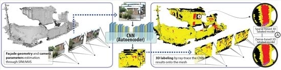
Considering these difficulties and the fact that today, only a few experiments with complex scenarios have been carried out, we present our methodology using ground images, since they can provide us all the façade details that aerial imagery might not be able to [35]. The purpose here is to delineate regions of interest of façade images and assign each of them to a particular semantic label: roof, wall, window, balcony, door and shop. After, these segmented features are used to link them to their respective geometries. In order to detect these features, six datasets with distinct architectural styles are used as training samples for a CNN model. Once trained, the artificial knowledge generated for each dataset is tested on an unknown scene in Brazil. The façade geometry is then extracted through the use of an SfM/MVS pipeline, which is finally labeled by ray-tracing analysis according to each segmented image.

Based on this workflow, in Section 2, we highlight the essential urban characteristics for the extraction of information through remote sensing, its challenges and the evolution of techniques. In Section 4, the details of the methodology and data adopted for the study are presented. In Section 5, we analyze the results in both categories: on two (quality of detection) and three dimensions (quality of 3D-labeling), as well as the training effects between the architectural style and the inference quality under an unknown one. Finally, in Section 6, our main conclusions and future prospects are given. Summarizing, we see three main contributions:

• An alternative methodology to detect façade features in common urban scenarios,
• An analysis under a wide variety of datasets, including a new one that does not follow usual architectural styles,
• An easy-to-use and less complex routine to label 3D models from 2D segmented images.

2. Related Work

Essentially, the results in the range of alternatives to reconstruct cities vary according to the definition of three main phases: (i) sensors and an appropriate measurement of the targets, (ii) processing and classification, according to a desired level of detail, and (iii) standardization in well-established formats, such as CityGML [36]. The following sections introduce the main works and methodologies in 3D reconstruction of buildings and façades, as well as the spatial and spectral characteristics usually found in these environments, which represent the great challenges of the area.

2.1. Urban Environments and Their Many Representations

The different categories of artificial coverage (man-made) constantly change in small fractions of space and time, often altered by humans, as well. Understanding the aspects of texture, geometry, material, architectural styles and coverage, among other physical properties, helps define the level of abstraction in the method to be developed [37]. The following sections briefly discuss some of the geometric aspects of buildings and their features, in order to contextualize the main factors for 3D modeling and reconstruction of these environments. For a more comprehensive reading, we recommend the work of [35].

2.1.1. Façade Features

The reconstruction of façades fulfills an important segment in inspecting and enforcing urban planning laws. For instance, the mapping of façade features (sometimes called openings and referenced here as façade features, such as doors, windows, balconies, gates, etc.) could assist in determining whether a new building can be erected in front of or at a given distance from a reference point. Burochin, J.P., et al. analyzed the façade characteristics in order to validate building constructions in accordance with French planning laws [38]. Not only is the geometry of buildings important, but their semantics are, as well. For the validation of urban plans, it is essential that windows and doors are not only geometrically represented, but also explicitly labeled as such [39].

Regardless of the imaging platform, artificial structures are easily distinguished from natural structures by their linear patterns. Areas with vegetation are generally heterogeneous, with non-uniform texture and typical spectral properties. Simple vegetation indexes, in this case, would separate adequately between vegetation and artificial cover [1,40]. However, in some cases, the vegetation is entirely mixed with urban environments, such as terrace-gardens or vertical gardens on balconies, aspects that make it difficult to classify them at the spectral level, but which could easily be categorized as buildings by complementing with volumetric information.

The perception of a building through the human visual system provides innumerable premises on which characteristics should be considered at first. As mentioned, linear structures are those that clearly expose an artificial structure and possibly a region of interest. In the real world, buildings are, in general, complex structures, with different orientations, slopes and roofs with different textures and compositions. Consequently, the analysis of applications involving the extraction of façades becomes less complex when the presence of objects in their surroundings is minimal [41,42].

In this study, however, we are interested in details of the building façades, and so far, there is no better way than close-range imaging to observe those details. The survey of urban data via terrestrial platforms benefits from the rich information collection, but it is a disadvantage by not allowing wide observation of the building structure, such as their internal architecture, roof and, depending to their height, only heir bottom part (Figure 1). However, as soon as these features are correctly mapped, other geospatial databases could equally benefit by merging of information.

The characteristics of doors and windows are pretty much distinguishable: a rectangular geometric pattern, sometimes occluded by vertical-gardens, cars, poles or other objects. The uniformity of the texture, structure and repeatability of such openings could be verified by the use of radiometric statistics, Histograms of Oriented Gradient (HOG) and the gradient accumulation profile, as in [38]. However, depending on the façade layout, the symmetry between the openings may not favor the respective method, unless the imaging is done by two different platforms.

In terms of architectural style classification, recent studies such as [43,44,45] have addressed the problem that we believe is the first stage in a 3D reconstruction methodology: first, to identify what we are dealing with: Is it a residential area? Is it industrial? The success of any method depends solely on the geometry of the façade, which lies exclusively in its architectural style. Van Gool, L., et al. discussed the importance of such pre-classification for a successful autonomous method [37].

Even though we will not approach the classification of styles in this work, we emphasize the importance of this stage. Instead, we aim to segment façade features without this “pre-classification” process by using Machine Learning (ML) techniques, which have been proven to be robust under complex scenarios, such as undefined architectural styles or areas occluded by obstacles. Our method considers not only multi-scale analysis, but it is also sensitive to the context, when objects obstruct doors or walls, for example, and are easily ignored by the neural model when the obstruction is small. In the following section, we list and discuss some of the main works focused on the extraction and reconstruction of urban environments.

2.1.2. Advances in 3D Urban Reconstruction

The use of high resolution images has been the most effective method for systematic monitoring in all contexts, be it forest, ocean or city. Understanding patterns of changes over time is, however, a task that requires enormous effort when executed manually. In addition, human touch is susceptible to failure and could require prior experience in target perception. As a matter of fact, so far, few studies have been carried out in the field of architectural style identification or façade feature extraction and reconstruction [46]. Research has reached a certain level of maturity today, with a variety of technologies for acquisition, high graphics processing and storage and dissemination of information that is available for the automatic operators.

The development of intelligent operators for image labeling can be categorized into model-free, model-based and procedural models. The first, classical segmentation methods such as normalized cuts [47], markov random fields [48], mean shift [49], superpixel [50] and active contours [51], do not consider the shape of objects or their spectral characteristics, which in practice, means they always fail in regions where the elements of the same façade do not share the same spectral attributes. Model-based or parametric model operators use a prior knowledge base, which together with segmentation procedures, provides more consistent results on a given region. However, this knowledge is finite and opens up new possibilities for failures when applied in regions with different characteristics. The third and last, procedural models, like grammar shape [52], comprise the group of rule-based methods, in which algorithms are applied to the production of geometric forms [33].

Image segmenters that have some intelligence usually carry issues with them, as well. First, it is necessary to configure and train the model, then make inferences about to what each pixel or region corresponds. Teboul, O., et al. proposed a grammar-based procedure to segment building façades, where a finite number of architectural styles was considered [33]. The proposed method was able to classify a wide variety of façade layouts and their features using a tree-based classifier, which improved the detection with only a small percentage of false negatives.

The grammar-based approaches, however, are normally formulated by rules that follow common characteristics, such as the sequentiality, which is normally present in “Manhattan-world” or European styles [53], where the shapes found seem to have lower geometric accuracy since the 3D model is generated, not reconstructed. Still, the outcomes of grammar-based approaches provide simplicity and perfectly resume the real scene. Other similar works, such as [54,55,56,57], have proposed equivalents solutions to the problem, but still having on the same deficiencies mentioned above.

In addition to procedural modeling, urban 3D reconstruction incorporates a new class of research, one based on physical (structural) measurements, which are comprised of measurements by laser scanners and MVS workflows (mainly). As far as we know, in this category lie the works that present the most consistent methodologies and results, which take into account the geometric accuracy, where the classification of objects can also be explored by their shapes or volume, in addition to their spectral information.

Jampani, V., et al. and Gadde, R., et al. respectively proposed a 2D and 3D segmentation-based Auto-Context (AC) [58] classifier [34,59]. The façade features were explored by their spectral attributes and then iteratively refined until the results were acceptable. The AC classifier applied in a urban environment is a good choice since it considers the vicinity contribution, which is essential in this particular scenario. The downside, however, is that in this case, the AC only succeeds when the feature detection (based on spectral attributes) is good enough; otherwise, it could demand many AC stages to get an acceptable output.

Unlike the approaches mentioned above, there are also lines of research that address the problem of 3D reconstruction over the mesh itself; for this reason, other structural data can be explored, such as LiDAR. The works in [41,60,61] presented different contributions, however with strictly related focuses. It should be noted, therefore, that the approaches in this line of research demand complex geometric operations, for instance regularities using parallelism, coplanarity or orthogonality. These operations usually have refinement purposes and also give the 3D modeling an alternative to acquire more consistent and simplified models.

Automatic 3D reconstruction from images using SfM/MVS workflows is challenging due to the non-uniformity of the point cloud, and it might contain higher levels of noise when compared to laser scanners. In addition to that, missing data is an unavoidable problem during data acquisition due to occlusions, lighting conditions and the trajectory planning [62]. The following mentioned papers explored what we understand as some of the best methodologies in 3D reconstruction, according to our established goals: exploring the texture first and then acquiring the semantic 3D model [63]. Martinovic, A., et al. proposed an end-to-end façade modeling technique by combining image classification and semi-dense point clouds [46].

As seen in Riemenschneider, H., et al. and Bódis-Szomorú et al., the respective approaches have motivated us in the sense that façade 2D information can be explored more thoroughly in order to improve its volumetry reconstruction [31,32]. Martinovic, A., et al., for instance, used the extracted façade features to analyze the alignment among them, where a simple discontinuity showed the boundaries between different façades [46]. Thereby, it could be used to pre-classify subareas, such as residential, commercial, industrial, and others. Sengupta, S., et al., Riemenschneider, H., et al. and Bódis-Szomorú et al., similarly explored different spectral attributes in order to discriminate the façade features as well as possible [31,32,64]. Moreover, the 3D modeling was later supported by these outcomes by performing a complex regularization and refinements over the mesh faces.

2.1.3. Deep-Learning

In terms of image labeling, years of advances have brought what is now considered a gold-standard in segmentation and classification: the use of Deep-Learning (DL). The technology is the new way to solve old problems in remote sensing [65]. It is one of the branches of Machine Learning (ML) that allows computational models with multiple processing layers to learn representations at multiple levels of abstraction. The term “deep” refers to the amount of processing layers.

These models have made remarkable advances in the state-of-the-art of pattern recognition, speech recognition, detection of objects, faces and others. To put it breifly, DL methods are trained to recognize structures in a massive amount of data using, for example, supervised learning with the concept of backpropagation (method commonly used in ML to calculate the error contribution of each neuron after each training iteration), where portions of what must be changed in each of their layers is corrected until “learning” occurs (error decay) [66].

In 1943, the first Artificial Neural Network (ANN) appeared [67]. With only a few connections, the authors were able to demonstrate how a computer could simulate the human learning process. In 1968, Hubel, D.H. and Wiesel, T. N. proposed an explanation for the way in which mammals visually perceive the world using a layered architecture of neurons in their brain [68]. Then, in 1989, the neural model started to get attention not only because of its results, but also for its similarities to the biological visual system, with processing and sensation modules.

LeCun, Y., et al. presented a sophisticated neural model for the recognition of handwritten characters, named Convolutional Neural Network (CNN), precisely by the successive mathematical operations of convolution on the image [27]. Since then, many engineers have been inspired by the development of similar algorithms for pattern recognition in computer vision. Different models have emerged and contributed to the evolved state of neural networks in the present day.

In the field of image analysis, the first reference to the use of CNNs for images was the AlexNet model [26]; that was when the technique began to be exhaustively tested and became a practical and fast solution for object classification. The typical CNN architecture is structured in stages. The first ones are composed of two types of layers: convolutional and pooling. Units in a convolutional layer are organized into feature maps or filters, where each unit is connected to a window (also called patch) in the feature map of the previous layer. The connection between the window and the feature map is given by weights. The weighted sum of the convolution operations is followed by a nonlinear activation function, called the Rectified Linear Unit (ReLU). For many years, activation in neural networks was composed of smoother functions, such as the $tanh\left(x\right)$ or $1/(1+e^{-x})$ sigmoid, but a recent study has shown ReLU to be faster when learning in multilayered architectures [66].

Neural models came to be used, then, in numerous applications in remote sensing [69], as in the analysis of orbital images [70,71], radar [72,73,74], hyperspectral [75,76] and in urban 3D reconstruction [77,78,79]. Although not focused specifically on the analysis of facades, excellent results have been reported in the classification of urban elements through the use of DL.

An example of this evolution can be observed in the annual PASCAL VOC [80] challenge, bringing together experts to solve classical tasks in computer vision and related areas. The applications range from recognition [26] to environment understanding, where the analysis is focused on the relationship between the objects themselves. Therefore, certain constraints could be imposed on the relation, for example between a pedestrian and street or vehicles in applications involving self-driving [29,30], such that distance and speed constraints could be imposed between these detected objects. Lettry, L., et al. used CNN to detect repeating features in rectified façade images, wherein the repeated patters were verified on a projected grid [81]. Then, it was used as a device to detect those regular characteristics and reconstruct the scene.

The DL as an automatic extractor of urban features is a scientific question of great interest to the community and also covers a limited number of works. The efforts, so far, show that there is progress in identifying facade features in specific architectural layouts, with well-defined, symmetrical and accessible modeling façades. The use of benchmark datasets is common and provides a wide overview of the extraction algorithms available today.

In [82], for example, DL was used for the identification of façade features on two online datasets, the eTRIMS and Ecole Centrale Paris (ECP) atasets, presenting similar results to those shown in this work. The VarCity project [32] (available at https://varcity.ethz.ch/index.html; accessed 22 June 2018), provides an accurate perspective of 3D cities and image-based reconstruction. The research involves not only studies of “how” to reconstruct, but how these semantic models could automatically assist in daily life events (e.g., traffic, pedestrians, vehicles, green areas, among others).

In this respect, our focus was to mitigate how this emerging technology could complement and guide studies such as the ones performed by VarCity [32] or virtualcitySYSTEMS [7], by presenting shortcomings, advantages, disadvantages and how it could fit in the 3D urban scope.

2.2. 3D Mapping around the World

Investigating the exact number of cities that actually use 3D urban models as a strategic tool in their daily lives can be a difficult task. However, [11] presented a consistent review of entities (industry, government agencies, schools and others) that make or made use of 3D maps beyond the visual purpose. Hence, only applications supported by 3D maps are, in fact, listed. Examples of such applications are the visibility analysis for security camera installation [18,83], urban planning [84,85], air quality analysis [86,87], evacuation plans in emergency situations [22] and urban inventories with database updating [88], among others.

Although the number of cities adopting this tool is uncertain, some of these are known for their technological advances and social development, an important indicator in the implementation of innovative projects. Countries such as the United States, Canada, France, Germany, Switzerland, England, China and Japan are among the leading suppliers of Earth observation equipment, for example, Leica Geosystems™ (Switzerland) laser systems, FARO™ (USA), Zoller-Fröhlich™ (Germany), RIEGL Laser Measurement Systems™ (Austria), Trimble Inc.™ (USA), TOPCON™ (Japan) and countless optical sensors used in ground and airborne surveys. It is natural, therefore, that these great providers also become references in conducting research in the sector.

In Germany, the so-called “city-models” were built with the basic purpose of assisting and visualizing simple scenarios or critical situations. At that time, these models did not have sufficient quality for certain analyses or permanent updating, making use of the old 2D registers for queries. In the end, the 3D models never became part of the register. The concept of urban 3D reconstruction has become, due to demand, a scientific trend in cartographic, photogrammetry and remote sensing almost everywhere in the world, especially in the aforementioned countries.

Naturally, new questions arose. How does one merge information already available in 2D databases with the ones in 3D? In certain circumstances, what is the limit on the use of 3D information? When is 2D already enough, and when is it not? Biljecki, F., et al. argued that all applications that require 2D information can be solved with 3D, but that does not make it a unique feature, but an optional one [11]. For example, de Kluijver, H. and Stoter, J. carried out a study of the propagation of noise in urban environments from 2D data [89]. Years later, in [90], the study was complemented with 3D information, showing considerable improvement in the estimation.

In Brazil, the Geographic Service Directorate (in Portuguese, Diretoria de Serviço Geográfico (DSG)) (available at http://www.dsg.eb.mil.br; accessed 22 June 2018) is the unit of the Brazilian Army responsible for establishing Brazilian cartographic standards for 1:250,000 and larger scales, which implies standardizing the representation of urban space for basic reference mapping. Recently, the National Commission of Cartography (in Portuguese, Comissão Nacional de Cartografia (CONCAR)) has put forward the new version of the Technical Specification for Structuring of Vector Geospatial Data (in Portuguese, Especificações Técnicas para Estruturação de Dados Geoespaciais Vetoriais (ET-EDGV)) [91], which standardizes reference geoinformation structures from the 1:1000 scale. The data on this scale serve as a basis for the planning and management of the urban geographic Brazilian space. In Brazil, the demand for 3D urban mapping is still low and faces challenges that go beyond its standardization.

As documented in this section, the state-of-the-art in automatic 3D urban reconstruction covers areas with moderate modeling, whose architectural styles are very specific, streets with large spacing or symmetry between facade elements, which makes the creation of automatic methods a bit more feasible [37]. In countries where there is a high density of buildings, such as Brazil, India or China, this factor is aggravated by the urban geometry. Many of the Brazilian cities do not have a specific style. In suburbs, for example, this factor can prove even more aggravating, where settlement areas or subnormal settlements (in Portuguese, favelas) are all built under these circumstances, with high density and sometimes erected irregularly or over risky areas.

Initiatives such as the TáNoMapa, by Grupo Cultural AfroReggae (available at https://www.afroreggae.org/ta-no-mapa/; accessed 22 June 2018), together with the North American company Google™, consist of mapping hard-to-reach areas such as streets with narrow paths and cliffs, among others, by the local residents. Such areas, in addition to being geometrically complex, require not only cooperation from the government, but also from the community that lives there, which due to social or security reasons, may require some consent.

Even though it faces many obstacles, Brazilian urban mapping is moving towards more sophisticated levels. In 2016, the National Civil Aviation Agency (in Portuguese, Agência Nacional de Aviação Civil (ANAC)) regulated the use of UAVs for recreational, corporate, commercial or experimental use (Brazilian Civil Aviation Regulation, in Portuguese, Regulamentos Brasileiros da Aviação Civil (RBAC), portaria E n° 94 [92]). The regulation, widely discussed with society, associations, companies and public agencies, establishes limits that still follow the definitions established by other civil aviation entities such as the Federal Aviation Administration (FAA), the Civil Aviation Safety Authority (CASA) and the European Aviation Safety Agency (EASA), regulators from the United States, Australia and the European Union, respectively [93]. Thus, close-range acquisitions through the use of UAVs became feasible and have fostered research in these fields.

3. Study Areas and Datasets

In

Table 1. Datasets for façade analysis and benchmarks. RueMonge2014 and Graz, ETH Zürich; CMP, Center for Machine Perception; eTRIMS, University of Bonn; ECP, Ecole Centrale Paris; SJC, São José dos Campos.

Name	Location	Arch.	Images	Labels	Rectified	PC Generation	Reference
RueMonge	France	Haussmannian	428	219	✗	✓	[32]
CMP	Multiple	Multiple	378	378	✓	✗	[94]
eTRIMS	Multiple	Multiple	60	60	✗	✗	[95]
ENPC	France	Haussmannian	79	79	✓	✗	[34]
ECP	France	Haussmannian	104	104		✗	[96]
Graz	Austria	Classicism, Biedermeier, Historicism, Art Nouveau	50	50	✓	✓	[97]
SJC	Brazil	Multiple	175	-	✓	✓	-

, seven different datasets are listed. The first six rows are online shared datasets, mainly used for evaluation and to perform benchmarks over different extraction models. They are then used in this study as diversified inputs, since each of them presents different façade characteristics. The last row is a dataset obtained exclusively for this work and used as test images. We aim to extract eight semantic classes: roof, wall, window, balcony, door, shop and, finally, two more, but unrelated to the façade, sky and background. Some of the datasets listed did not provide all eight classes, and in some cases, their annotations had to be adapted.

RueMonge2014: The RueMonge2014 dataset was acquired to provide a benchmark for 2D and 3D façade segmentation and inverse procedural modeling. It consists of 428 high resolution images, with the street-side view (overlapped) of the façade, with Haussmannian architecture, for a street in Paris, Rue Monge. Together with the 428 images, a set of 219 annotated images with seven semantic classes was also provided. Due to the geometry of acquisition, the dataset offers the possibility to generate a 3D reconstruction of the entire street scene.

Center for Machine Perception (CMP): CMP consists of 378 rectified façade images of multiple architectural styles. Here, the annotated images have 12 semantic classes; among them, some façade features such as pillars, decoration and window-doors were considered as being part of the wall (for pillars and decoration) and window (window-doors). Then, we adapted the CMP dataset by unifying its classes and their respective colors.

eTRIMS: The façades in this set do not have a specific architecture style and sequence, as in the previous dataset. The eTRIMS provides 60 images, with two sets of annotated images, one with four semantic classes (wall, sky, pavement and vegetation) and another with eight (window, wall, door, sky, pavement, vegetation, car and road). For our project, we chose the last, but adapted it to window, wall and door features only. The other classes were considered as background.

ENPC: The ENPC dataset provides 79 rectified and cropped façades in the Haussmannian style. The annotations, however, are shared not in image format, but in text, which also had to be adapted to the seven classes and colors defined in this work.

Ecole Centrale Paris (ECP): Just like RueMonge2014, the 104 façade images provided by ECP are in the Haussmannian style, but the images are rectified, with cropped façades. In some cases, the classes’ windows, roof and walls were not perfectly delineated, which may be considered noise by supervised neural models. The same issue can also be found in the ENPC dataset. Even though we noticed the problem, no adaptation was performed.

Graz: The Graz dataset consists of multiple architectural styles, selected from the streets in Graz (Austria), rectified with the same seven semantic classes defined in RueMonge2014.

São José dos Campos (SJC): The SJC dataset consists of buildings in a residential area in São José dos Campos, São Paulo, Brazil. Like most of the country, the architectural style throughout this city is not unique, often diverging between free-form and modern styles. This set consists of 175 sequential images, overlapped, and taken at the same moment.

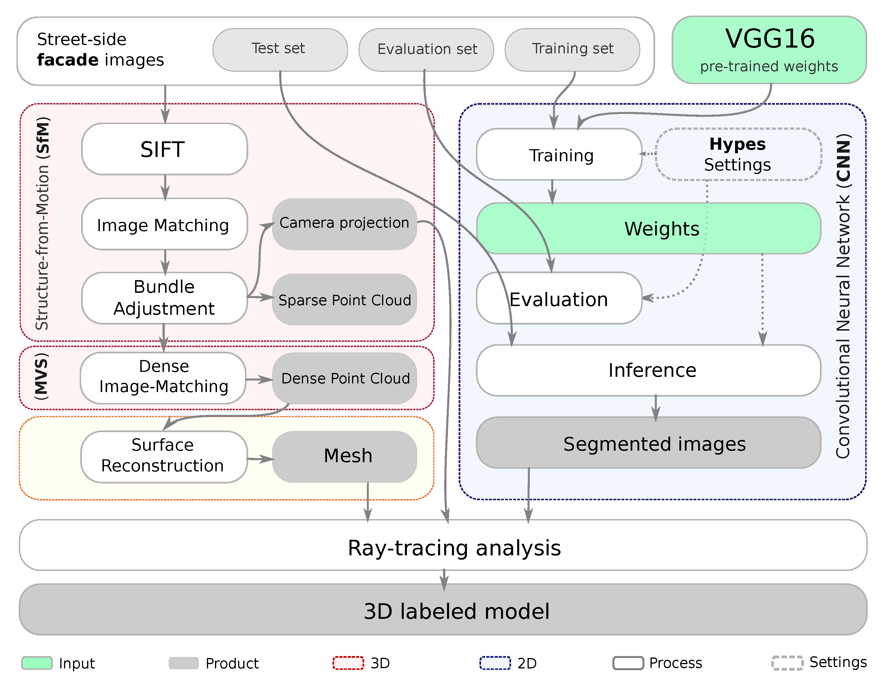
4. Methodology

The complete methodology of this case study, as shown in Figure 2, consists of three stages: a supervised CNN model for semantic segmentation (blue); scene geometry acquirement (3D reconstruction) through the SfM pipeline (red); MVS (also in red); Post-processing (yellow); and 3D-labeling through ray-tracing analysis. The boxes in gray represent the products, delivered at different steps of the workflow. The following sections, therefore, are presented according to this sequence.

4.1. Façade Feature Detection

4.1.1. Training Set

Each of the six datasets has been divided into three different subsets: training, validation and testing. Eighty percent of the annotated images were used for training and 20% for validation. Only RueMonge2014 had a non-annotated set of images (209), which was used for testing. Due to the small number of training samples, no set of test images was used for the other group of data. Instead, a new acquisition with similar geometry as RueMonge2014 was performed in the city of São José dos Campos (SJC), São Paulo, Brazil. The images will be used only for testing, whereas each of the mentioned datasets are used for training.

4.1.2. Neural Model

The classic DL architectures used in visual data processing can be categorized in Autoencoders (AE) and CNN architectures [69]. An AE is a neural network that is trained to reconstruct its own input as an output. It consists of three layers: input, hidden and output. The hidden layer takes care of all operations behind this model; here, the weights are iteratively adjusted to become more and more sensitive to the input [98]. The CNNs, on the other hand, take advantage of performing numerous convolution operations in the image domain, where a finite number of filters is repetitively applied in a downsampling image strategy, which allows the analysis of the scene at different orientations and scales.

The decoder is seen as a component that interprets chaotic signals as something intelligible, akin to the human senses. For example, it would be like the equivalence between a noise (signal) and a person talking in a known language (interpreted signal by our brain), radiation (signal) and the perception of being under a garden with flowers and animals (brain interpretation of this same radiation), etc. Similarly, we use only one decoder since our purpose is the interpretation of images, emulating what would be the the visual sense. The neural architecture presented by [30], for instance, used 3 different decoders with 3 different tasks in a way that real-time application could be performed. The use of multiple decoders for our purpose, however, is not interesting due to the useless computational demand and unnecessary processing.

Our final network is then composed of an encoder with a VGG16 network and a decoder with a Fully Convolutional Network (FCN) architecture [99]. The encoder corresponds to the same topological structure of the convolutional layers of VGG16 [100], where it was originally composed of 13 convolutional layers, followed by their respective pooling and Fully-Connected (FC) layers. Our encoder, however, had its FC replaced by a $1\times 1$ convolutional layer, which takes the output from the last pooling layer (called pool5) of size $39\times 12\times 512$ and generates a low resolution segmentation of size $39\times 12$ [30]. This change makes the network smaller and easier to train [29]. Then, the FCN decoder takes the $39\times 12$ matrix as an input for its 3 convolutional layers, which finally performs the upsampling operation, resulting in the pixel-wise prediction.

4.1.3. Multi-View Surface Reconstruction

Our input is a set of images that were initially fed to standard SfM/MVS algorithms to produce a 3D model. Not all datasets listed in Table 1 have properties that could allow the application of SfM/MVS. For instance, random, rectified and cropped images are not overlapped or, at least, were not taken at the same moment. Only RueMonge2014 was able to be used to run this experiment. A case where random images were taken at different times was proposed by [101], but not used in this work.

The façade geometry acquirement was carried out by the common SfM pipeline, which includes the camera parameters estimation and the point cloud densification by the MVS technique. For this task, we have used the Agisoft™ PhotoScan${}^{\circledR }$.

The geometric accuracy in this study corresponds to the proximity between the reconstructed model and the point cloud, not necessarily to the positional part $(X,Y,Z)$. In this case, it was assumed that the point cloud had previously proven positional accuracy. It was beyond the scope of this work to analyze adjustments or positioning issues.

4.2. 3D Labeling by Ray-Tracing Analysis

At this point, two products are achieved: the classified façade features (2D image segmentation) and their respective geometry (mesh). The idea here is to merge each feature with its respective geometry, and that can be done by analyzing the ray-tracing of each image with respect to their camera projection (estimated during the SfM pipeline) onto the mesh.

Often used in computer graphics for rendering real-world scenarios, such as lighting and reflections, ray-tracing analysis mimics real physical processes that happen in nature. A energy source emits radiation at different frequencies of the electromagnetic spectrum. The small portion visible to human eyes, called the visible region, travels straight in wave forms, and it is only intercepted when it encounters a surface in its trajectory. Such a surface has specific physical, chemical and biological properties. Such characteristics define the behavior of radiation under its structure, determining exactly what we see.

Each façade image, in essence, is the record of the reflection of electromagnetic waves in a tiny interval of time, captured by a sensor at a certain distance and orientation. Once the camera’s projection parameters (focal length, center of projection, orientation, among others) are known, the original images used for its estimation during SfM are replaced by the segmented ones. Thus, the “reverse” ray-tracing process can then be performed.

It is evident, therefore, that the rays’ trajectory from the images can intersect one another. Because of that, different rays can reach an identical point on the mesh, what in fact creates questions such as “which class should be assigned to each individual mesh facet?”. The work in [32] proposed the Reducing View Redundancy (RVR) technique, where the number of overlapped images was reduced, which does not fit to our purpose, since the greater the number of overlaps, the better the labeling (more classes to choose). That could be solved through the application of a simple rule such as the mode (most frequent class) or even a smarter decision rule (e.g., choose the class where the segmented image’s ray had the highest accuracy during the CNN inference), but we have noticed that a simple mode operation can provide sufficient labeling.

The external camera parameters are initially estimated during the bundle adjustment in the scope of the SfM procedure. Thus, each image has its position C and orientation R, consisting respectively of the camera projection center located at the origin of the 3D coordinate system $C=(C_X,C_Y,C_Z)$ and rotation matrix $R=(R_X,R_Y,R_Z)$. The origin of a certain ray, then, is all camera projection center C, with its direction given by R. Considering no optical blur, distortion or defocus, a point $C_i$ is mapped to a point in the image plane $(u,v)$ by:

$$\begin{array}{c}\hfill p_i(u,v,f)=\frac{f}{Z}\left(\begin{array}{c}X\\ Y\\ Z\end{array}\right),\end{array}$$

(1)

where f is the known focal distance (left in Figure 3), $u=f\frac{X}{Z}$ and $v=f\frac{Y}{Z}$.

Knowing the pixel class from the incident ray, the mesh triangle is finally labeled as such. If more than one ray reaches the same point on $p^{\prime }$, then the face is labeled by the most frequent class from the $C_n$ rays (right in Figure 3).

5. Results and Discussion

5.1. Performance

As a supervised methodology, the DL requires reference images (also referenced as annotation, labels or ground-truth images), which means the methodology is extensible for images of any kind, but it will always require their respective reference. On the other hand, the same neural model could fit any other detection issue, for instance in the segmentation of specific tree species in a vast forest image, as soon as a sufficient amount of training samples is presented.

All the source-code regarding DL procedures was prepared to support GPU processing. Unfortunately, the server used during all the experiments was not equipped with such technology, increasing training time significantly (

Table 2. Training attributes and performance.

Dataset	No. of Iterations	Average Resolution	Training (hours)	Inference (seconds per Image)
RueMonge2014	50 k	800 × 1067	172.46	5.4
CMP	50 k	550 × 1024	135.25	4.45
eTRIMS	50 k	500 × 780	83.57	3.52
ENPC	50 k	570 × 720	53.47	2.01
ECP	50 k	400 × 640	38.32	3.13
Graz	50 k	450 × 370	29.27	2.05
SJC	-	1037 × 691	-	4.2

).

The DL source-code was mainly developed under the Tensorflow™ library (available at https://www.tensorflow.org/; accessed 22 June 2018) and adjusted to the problem together with other Python libraries. Except for the 3D tasks in PhotoScan, the source-code is freely available on a public platform (for access and further explanations, please, contact us) and can be easily extended. For training and inferences, we used an Intel${}^{\circledR }$ Xeon${}^{\circledR }$ CPU E5-2630 v3 @ 2.40 GHz. For SfM/MVS and 3D-labeling, with respect to the RueMonge2014 and SJC datasets, we used an Intel${}^{\circledR }$ Core™ i7-2600 CPU @ 3.40 GHz. Both met our expectations, but we strongly recommend machines with GPU support or alternatives such as IaaS (Infrastructure as a Service).

5.2. Experiments

The experiments in this work were divided into the 2D and 3D domains. To mitigate the influences of each dataset, or the influences of the model under each specific architectural style, we split the 2D experiments into three different CNN trainings. First, all six online datasets listed in Table 1 were trained and inferred independently. Second, the knowledge reached from the respective datasets was used for testing under SJC, which has a completely undefined architectural style. Third, all datasets were then put together, and a new training was performed under SJC (

Table 3. Experiments performed in this work. The term “independent” means the dataset or inference was made using only one dataset for training or prediction.

#	Domain	Dataset	Inferences	Goal
1	2D	Independent	Independent	Evaluate the performance of the neural model according to each dataset
2	2D	Independent	SJC	Evaluate the performance of the neural model according to the SJC dataset, where the inferences are made six times, using the datasets’ knowledge separately
3	2D	All-together	SJC	Evaluate the performance of the neural model according to the SJC dataset, where only one inference is made, using all knowledge together
4	3D	RueMonge2014	-	Evaluate how accurate the 3D-labeling is according to the point cloud density, under a known dataset
5	3D	SJC	-	Evaluate how accurate the 3D-labeling is according to the point cloud density (sparse and dense), under an unknown dataset

). In the 3D analysis, the experiments consisted of permuting the density in the point cloud, allowing us to know how the number of points affects the 3D-labeling and how many are actually necessary to acquire reliable geometry.

5.3. Image Segmentation

5.3.1. Inference over the Online Datasets

As mentioned in Section 4.1.1, 20% of annotated images from each dataset were used to evaluate the model. The set consists of pairs of original and ground-truth images, which were not used during the training. The experiments carried out in this study were done individually. First, we discuss the quality of the segmentation through the use of CNN for each dataset (following the sequence according to Table 1), then we highlight our impressions of the detection of objects and in which situations it might have failed or still need attention. We proceed with the analysis of the geometry extraction and the quality of the 3D-labeled model.

Figure 4 below shows the neural network training results. It is simple to notice a similar behavior for all training datasets, except for the weight loss, the decay of which is strongly related to the image dimension. The demand for the learning of all features (generalization) is greater and varies among them. Accuracy and cross entropy, on the other hand, had progressed mostly from 0–10 k iterations, stabilizing near 90% and 0.1 thereafter, respectively. Thirty thousand iterations were sufficient to reach similar results for all datasets (as we will show later in the visual inspection). However, RueMonge2014, ENPC and Graz still had high error rates, which means that not all classes could be detected or clearly delineated.

Then, in

Table 4. Inference accuracy over the online datasets. Var.—Variance; StD.—Standard Deviation. The values in bold, expose the best datasets according to the Accuracy and F1-Score metrics.

Dataset	Accuracy	Var.	StD.	F1-Score	Var.	StD.
RueMonge2014	0.93	0.008	0.090	0.22	0.000	0.027
CMP	0.87	0.005	0.073	0.73	0.001	0.043
eTRIMS	0.92	0.000	0.027	0.82	0.000	0.017
ENPC	0.85	0.001	0.031	0.76	0.000	0.009
ECP	0.91	0.000	0.021	0.90	0.000	0.014
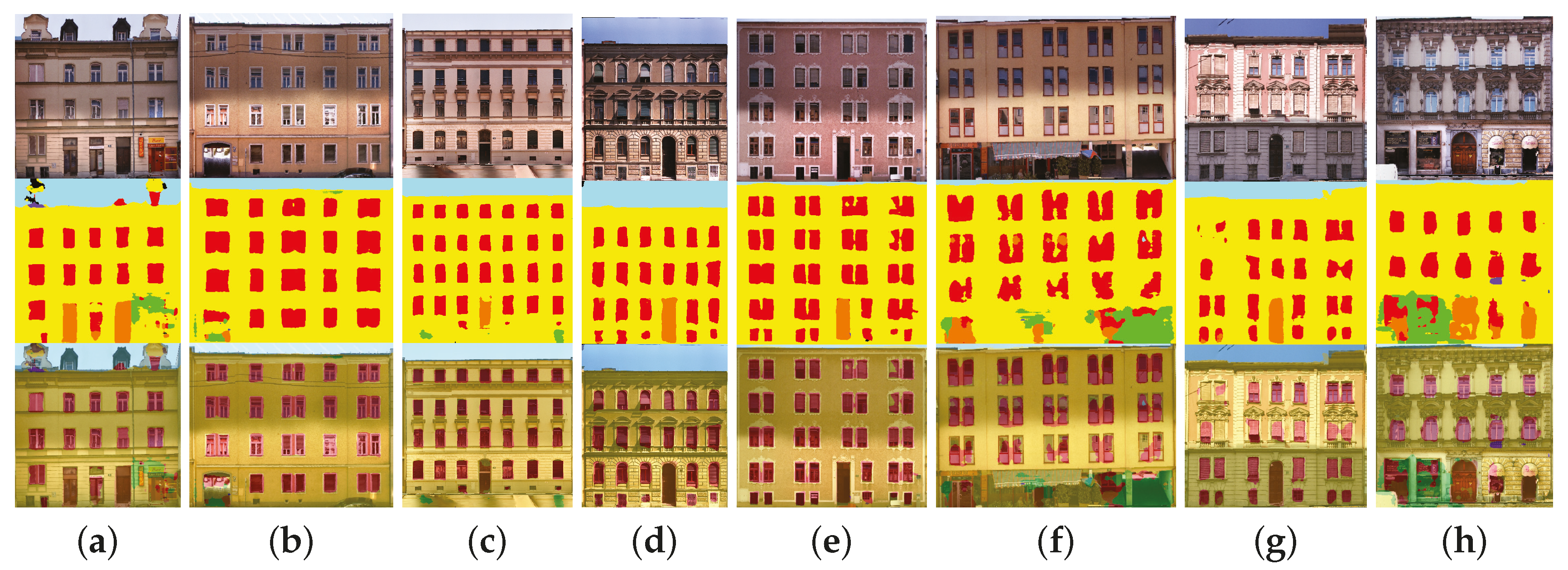
Graz	0.85	0.014	0.117	0.65	0.000	0.023

, we list the accuracies and F1-scores (expressing the harmonic mean of precision and recall) for each online dataset. The values reveal how good the segmentation was according to the correct assignment (accuracy) and object delineation (precision). RueMonge2014 presented the best results among the datasets. However, although its accuracy was superior, its F1-score was far below the others. This demonstrated an excellent inference of the region in which the object was found, but unsatisfactory regarding its delineation. Thus, the predictions with the ECP dataset presented better quality in both metrics. The others had similar results to ECP. The columns in red and green represent the variance and standard deviation, respectively, for the validation samples.

Figure 5 shows the inferences from RueMonge2014 over the validation set. Instead of showing only a few example results, we decided to expose as much of each dataset as possible, to allow the reader to better understand how the neural model behaves according to different situations. Here, we positively highlight two aspects. First is the robustness of the neural model in the detection of façade features even under shadow or occluded areas, such as in the presence of pedestrians or cars. This aspect has been one of the most difficult issues to overcome due to the respective obstacles being dynamic and difficult to deal with, especially with the use of pixel-wise segmenters. The second aspect is that at 50 k, all images presented fine class delineation, exceeding our expectation. Only in a few situations were the inferences unsatisfactory.

The annotated images from RueMonge2014 did not cover the entire scene, e.g., sky, street intersections, background buildings (far from main façades), etc, were annotated as background. This means that when presented to the CNN, all those features (sky, street intersection, etc.) annotated as background are going to be trained as background, as well. Therefore, whenever an intersection or sky appears, the neural model treats it as being background. The problem is that only half of the feature will be assignd as background, which is not the case with the other half. The same behavior was visible in other classes. For instance, when an annotated façade appears only partially in the validation set (clear in Figure 5f,h,i), the model will act as if the façade that it was trained to detect was not present in this image, only a part of it. That supervised neural model is strongly related to the context in which it has been trained. If a feature appears in the image, but only part of it is detected, the segmentation will fail because of the incomplete context.

Both CMP (Figure 6) and eTRIMS (Figure 7), present classes beyond those already analyzed in this study. The classes that are not related were ignored and had their annotations adapted to the problem, as well as their colors. For example, CMP has annotations for pillars and wall decorations, which we considered as a single class: wall. For eTRIMS, in addition to the classes not approached in this study, there were façade features where the annotation belonged to only one class, e.g., the roof in eTRIMS is annotated as being wall. For that reason, images with a roof had it assigned as wall and, consequently, assumed as a True Positive (TP) (Figure 7). Among the six façade features of interest, only three in eTRIMS were considered: window, door and wall. For CMP, all classes were considered, but some annotations were unified in order to make the inputs consistent for training.

The level of accuracy for all sets made the use of CNN the best of all alternatives. However, when looking closely at the results, we notice some remaining issues that could be investigated in a possible future work. For example, when objects such as trees appear right in front of the facade, they might add disturbances in the training phase. In the case it was a tree, it could be annotated as either vegetation or part of the façade itself (for example, note the differences between Figure 7b and Figure 8b). We understand that the lack of information in the first figure is the best inference, and in this case, the neural model is actually right: there is a façade with an unknown object in front of it.

However, in cases such as in Figure 8b, the façade inference is noisy or unreadable, which is not the case in Figure 8h, where the disturbance is minimal.

In addition to ENPC, ECP also presented inconsistencies in some of its annotations. The missing roof-parts in Figure 9a–f are expected behaviors since the annotations from the training sets do not consider these objects as being part of the roof. However, the learning happens for most of the features and should not be a problem since the neural model will identify the main content in the image.

No online datasets does have any certificate of quality. When checking the annotated images of some of them, there is a high degree of inconsistency between the annotations. This implies incorrect segmentation (see overlapping images, detail on the roofs) according to the real scenario, not to the validation set. This means the validation metrics might present some inconsistency, since they are calculated according to the validation (annotated) images. The inferences for CMP reached 0.87% accuracy, 0.92% for eTRIMS, 0.91% for ECP, 0.85% for ENPC and 0.85% for Graz. All those sets had similar inferences and errors, regardless of the predominant architectural style.

Among the inputs, Graz has the smallest number of images, but the spectral variability is clearly greater when compared to the others. The symmetry between windows, however, was pretty much the same in CMP, ECP and ENPC. We saw then that the results for Graz (Figure 10) did not change much from what was seen with the other datasets.

5.3.2. Inference over the SJC Dataset

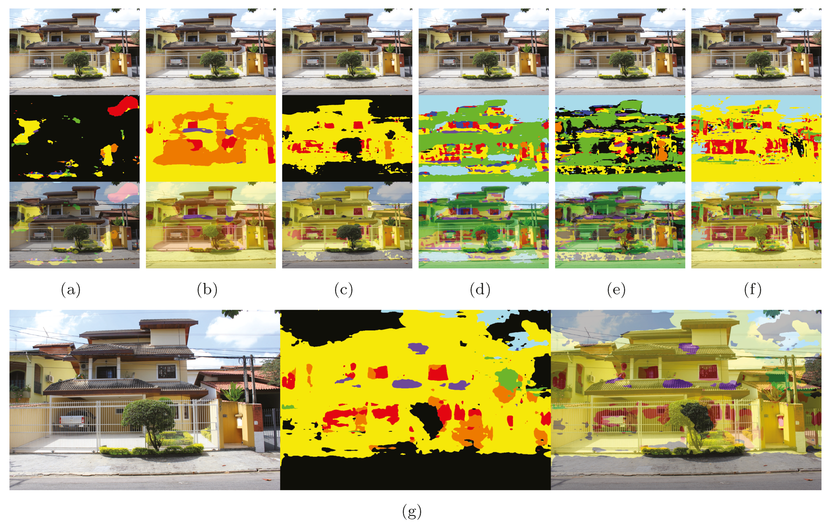
The idea behind the usage of the SJC dataset is simple: to observe how the neural network reacts to an unknown architectural style after being trained with different ones. The outcome could then provide insights into how the training set should look for the detection of façades of any kind. Figure 11 shows the results after presenting SJC images to a different version of the training data (knowledge).

Figure 11a–f shows the respective results from the datasets listed in Table 1 (online). When looking at these results as seen in the figures, we can safely conclude that these are incorrect and inaccurate segmentations. The fact is that in environments having a diversity of objects, any other segmentation and classification methods would have a certain imprecision. The operation of a CNN is not to perfectly delineate an object, but to provide hints (as close as possible) to where a given object is located in the image. This shows us that in order to extract precise parameters, such as the height and area of a feature, a post-processing phase should certainly be conducted on the CNN beforehand.

Going through one problem at a time, we notice that, firstly, there is a need to define a background class in supervised approaches. Using RueMonge2014 knowledge, the inference process was not able to segment properly even under the most common feature: wall. It is unlikely that some knowledge generalized it to sky, sidewalk and street, especially when there is no general class that represents too many objects in the scene (Figure 11c). When the class is annotated correctly such as sky, we see proper segmentation: that is the case with ECP (Figure 11d), ENPC (Figure 11e) and Graz (Figure 11f). When it is not, the inference is poor or average: which was the case with RueMonge2014 (Figure 11a). Features in RueMonge2014 were pretty much dependent on local architectural style. In general, we see eTRIMS as the dataset with the most similar features for SJC. Despite being trained with only four classes, including background, the results have shown a certain level of intelligence in detecting sidewalks and streets as being part of the background, as well as for sky and vegetation.

Therefore, when using a supervised neural network, it is evident that the arrangement of the annotations can affect the inference, either positively or negatively; for instance, annotations for all the sky coverage instead of only part of it, or sidewalks and street as background, in cases that it is not a desired feature.

In Figure 11g, we see the summarized contributions of each dataset, when used together in the training. For instance, eTRIMS was the only one sensitive to sidewalk and street, and balconies were only detected in CMP, even though this was incorrectly segmented. Meanwhile, the results for unknown features were understandable and expected. We believe that with the addition of more classes (e.g., gate), improvements to the annotation process and an increase in the number of training epochs, the better the results of the inferences would be.

Table 5. Inference accuracy over the SJC data. The last row corresponds to the accuracy with the knowledge of all trainings together. The values in bold, expose the best datasets according to the Accuracy and F1-Score metrics. When together, the quality metrics increased due to the better generalization of the neural network, as it has received a bigger amount of images.

Knowledge from...	Accuracy	Var.	StD.	F1-Score	Var.	StD.
RueMonge2014	0.31	0.003	0.054	0.10	0.000	0.014
CMP	0.36	0.006	0.080	0.16	0.001	0.043
eTRIMS	0.45	0.001	0.037	0.17	0.000	0.017
ENPC	0.29	0.001	0.031	0.19	0.000	0.009
ECP	0.25	0.012	0.016	0.17	0.000	0.014
Graz	0.37	0.006	0.078	0.18	0.000	0.023
All together	0.55	0.011	0.107	0.30	0.000	0.020

below shows the accuracy overview for each individual learned feature (knowledge) over the SJC dataset.

Both visually (Figure 7) and in the table, it is evident that eTRIMS was better suited to deal with the architectural style seen in the SJC dataset. It was expected, however, that the values for accuracy and precision would be low, due to the characteristics (similarities) of the SJC dataset. However, eTRIMS consists of unrectified façades, lacks symmetry between doors and windows and presents specific architectural styles, characteristics that bear similarity with the SJC images. When the data collection was united (all-together dataset), the accuracy was increased, but without improvements to the correct delineation of the objects.

5.4. 3D Labeling

The quality of the reconstructed surface (mesh) is highly dependent on the density of the point cloud and the method of reconstruction. Very sparse point clouds can generalize feature volumetry too much, while very dense point clouds can represent it faithfully, and the associated computational cost will also increase. Therefore, there is a limit between the quality of the 3D-labeled model and the point cloud density, which falls in the question: How many points do we need to fairly represent a specific feature? Features that are segmented in the 2D domain might perfectly align with their geometry, but imprecisions between the geometric edges and the classification may occur. These impressions are directly related to the mesh quality.

Table 6. Ray-tracing performance for geometry classification.

Dataset	Point	No. of Faces	3D Reconstruction: SfM	Ray-Tracing
	Cloud Density	(Triangles)	(min)	(s)
RueMonge2014	Sparse	1,072,646	21.4	12.42
RueMonge2014	Dense	9,653,679	46.4	27.13
SJC	Sparse	800,000	13.6	20.89
SJC	Dense	3,058,329	35.5	41.12

shows how the ray-tracing procedure performed. It was responsible for connecting each segmented feature to its respective geometry.

In order to illustrate the influences of the point cloud density on the quality of 3D-labeling, Figure 12 shows the result for the RueMonge2014 dataset. Only sparse and dense point clouds were tested. However, we would like to explore the limits between the number of points and the geometric accuracy in a future work.

Figure 12d,g, we highlight how well the point cloud density could represent a labeled 3D model. Assuming a hypothetical situation where area information or window height is required to estimate the brightness of the building (indoor and outdoor), the estimation of these parameters should be as close as possible to reality. Therefore, the height and area obtained from the mesh, as in the respective figures, may be inaccurate. Martinovic, A., et al. and Boulch, A., et al. proposed a post-processing procedure, in which the façade has its features simplified by the so-called parsing, where most of the time, grammar-based approaches [52] are used [46,57]. Perhaps the post-processing phase is essential in applications where precise geometric information is required, but we have to ensure that the geometric accuracy does not get penalized.

The 3D reconstruction performed by SfM is based on the identification of corners and image analysis, with the purpose of checking for correspondence and acquiring overlapping pairs. For this reason, the spectral properties from the urban elements influence the reconstruction process directly. For example, surfaces where the texture is too homogeneous or specular properties are present tend not to be detected by the algorithm and end up represented as a lack of information on the 3D model. Similarly, the MVS technique (responsible for dense 3D reconstruction) is equally dependent on the homogeneity of the objects.

Unfortunately, we can see many of these spectral properties over SJC façades. The textures related to walls are often uniform, with windows completed in glass. Besides, the geometry of acquisition did not contribute in this case. As seen in Figure 13a–c, all over the street, there are always gaps between the gate and the façade itself. These gaps often imposes problems during and after the reconstruction. As a consequence, we have many them among the important artifacts that could be determinant when trying to identify features in a semantic system. Hence, in order to fully map buildings through the use of SfM/MVS, the imaging of these areas, at least in Brazil, should be complemented by aerial imagery with the aim of targeting these areas (as presented and discussed in Section 2.1.1, Figure 1). The final 3D reconstruction, however, was moderate as the segmentation in the 2D domain.

Figure 14a (overview), Figure 14b,d (reconstruction details from sparse point cloud), and Figure 14e (reconstruction details from dense point cloud) correspond to the same residential building as the previous picture, the geometry of which is characterized by high walls and gates. Trees and cars appear in most of the images. These objects serve as obstacles, especially in terrestrial and optical campaigns. Of course, this depends solely on the imaged region. In the case of RueMonge2014, for example, while pedestrians, cars and vegetation act negatively in the reconstruction, the texture of the façade contributes positively. This makes the final 3D model penalized, but still, it is an acceptable product. As we can see in Figure 13 and Figure 14, however, not only the texture, but also the houses’ geometry and the frequent presence of obstructing objects negatively affected the reconstruction. In Figure 14c, a different area with very poor labeling is shown. Although the gate has been assigned partially correctly, the features here are mostly unreadable.

6. Conclusions

Increasingly, the research regarding façade feature extraction from complex structures, under a dynamic and difficult environment to work in (crowded cities), represents a new branch of research, with perspectives in the areas of technology, such as the concept of smart cities, as well as the areas of cartography, toward more detailed maps and semantized systems. In this study, we have presented an overview of the most common techniques, instruments and ways of observing structural information through remote sensing data. Besides, we also presented a methodology to detect façade features by the use of a CNN, incorporating this detection of its respective geometry through the application of an SfM pipeline and ray-tracing analysis.

We focused mainly on aspects such those aforementioned techniques and their computational capability in detecting façade features, regardless of architectural style, location, scale, orientation or color variation. None of the images used in the training procedures underwent any preprocessing whatsoever, keeping the study area as close as possible to what would be a common user dataset (photos taken from the street).

In this sense, the edges of the acquired delineated features show the robustness of the CNN technique in segmenting any kind of material, at any level of brightness (shadow and occluded areas), orientation or with the presence of pedestrians and cars. Considering that the values achieved for the individual datasets were above 90%, we can conclude that CNNs can provide good results for image segmentation in many situations. However, being a supervised architecture, the network has to pass through a huge training set, with no guarantees of good inputs, in order to get reliable inferences. When applied over unknown data, such as the experiment on the SJC data, we noted that the neural network failed, except in regions where the façade features share similar characteristics, though such occasions were rare.

This was the first of many studies directed towards the automatic detection of urban features focusing on complex and “non-patterned” environments. The methodology is consistent, but some traditional issues still remain, such as real-time detection and reconstruction, as well as façade geometry simplification and standardization.

As future prospects, we would like to explore aspects such as the use of non-supervised models, separate tasks such as pre-classification of architectural styles and a mix of different DL techniques to deal with specific scenarios, such as the chaotic arrangement of urban elements. Being our first case study, the methodology presented is highly dependent on the quality and number of images for training. The power of the generalization of the neural network occurs as the training sets are large and have good resolutions. Besides, this case study has shown the robustness of CNN in complicated situations, and we believe that efforts directed towards post-processing techniques could make the final 3D-labeled model even more accurate.