Deep&Dense Convolutional Neural Network for Hyperspectral Image Classification


Hyperspectral Computing Laboratory (HyperComp), Department of Computer Technology and Communications, Escuela Politecnica de Caceres, University of Extremadura, Avenida de la Universidad sn, E-10002 Caceres, Spain
*
Author to whom correspondence should be addressed.
†
These authors have contributed equally to this work.
Remote Sens. 2018, 10(9), 1454; https://doi.org/10.3390/rs10091454
Submission received: 17 July 2018
/
Revised: 28 August 2018
/
Accepted: 9 September 2018
/
Published: 11 September 2018
(This article belongs to the Special Issue Recent Advances in Neural Networks for Remote Sensing)
Abstract
:Deep neural networks (DNNs) have emerged as a relevant tool for the classification of remotely sensed hyperspectral images (HSIs), with convolutional neural networks (CNNs) being the current state-of-the-art in many classification tasks. However, deep CNNs present several limitations in the context of HSI supervised classification. Although deep models are able to extract better and more abstract features, the number of parameters that must be fine-tuned requires a large amount of training data (using small learning rates) in order to avoid the overfitting and vanishing gradient problems. The acquisition of labeled data is expensive and time-consuming, and small learning rates forces the gradient descent to use many small steps to converge, slowing down the runtime of the model. To mitigate these issues, this paper introduces a new deep CNN framework for spectral-spatial classification of HSIs. Our newly proposed framework introduces shortcut connections between layers, in which the feature maps of inferior layers are used as inputs of the current layer, feeding its own output to the rest of the the upper layers. This leads to the combination of various spectral-spatial features across layers that allows us to enhance the generalization ability of the network with HSIs. Our experimental results with four well-known HSI datasets reveal that the proposed deep&dense CNN model is able to provide competitive advantages in terms of classification accuracy when compared to other state-of-the-methods for HSI classification.
1. Introduction
The goal of this section is to introduce a new deep neural model for remote sensing data processing, aimed at conducting classification of hyperspectral images (HSIs). To present the rationale and objectives of this work, this section will introduce the problematic around hyperspectral data processing, focusing on the classification task, and indicating the most widely-used classification methods and algorithms. In particular, this section will highlight the use of deep learning (DL) strategies for data analysis, highlighting those methods based on convolutional neural networks (CNNs) as the current-state-of-the-art of DL field. Also, this section will point out the limitations of these methods when working with complex HSI datasets and very deep architectures, describing the new improvements developed on very deep neural networks. Finally, the section enumerates the goals and contributions of the current work.
1.1. Hyperspectral Imaging Concept and Missions
The combination of spectroscopy and photography technologies in current imaging spectrometers allows for the acquisition of spatial-spectral features capturing the visible and solar-reflected infrared (near-infrared and short-wavelength infrared) spectrum at different wavelength channels for different locations in an image plane. Particularly, in the remote sensing field this image plane is usually obtained over an observation area on the surface of the Earth by airborne and spaceborne spectrometers [1] which produce large amounts of data per hour, usually close to the Gigabytes of information, with improved spatial resolution also. In the category of aerial spectrometers we can highlight, for instance, the Airborne Visible InfraRed Imaging Spectrometer (AVIRIS) [2], which records information in the range of 0.4–2.45 m in 224 spectral bands, providing continuous spectral coverage at intervals of 10 nm over the spectrum. Another well-known aerial spectrometer is the the Reflective Optics System Imaging Spectrometer (ROSIS-3) [3], which covers the region from 0.43–0.86 m with more than 100 spectral bands at intervals of 4nm. Other aerial spectrometers are the Hyperspectral Digital Imagery Collection Experiment (HYDICE) [4], the HyMAP [5,6], the PROBE-1 [7] or the family of spectrometers composed by the Compact Airborne Spectrographic Imager (CASI), which capture information in the visible/near infrared regions, and its related SASI and TASI, which capture information in the short wave infrared and also in the thermal infrared, respectively [8,9,10]. Focusing on spaceborne sensors, we can highlight the Earth Observing-1 (EO-1) Hyperion [11,12], which also records information in the range 0.4–2.5 m with 10nm spectral resolution, obtaining data cubes with 220 spectral bands. Other spectrometers allocated on satellite-platforms are the Moderate Resolution Imaging Spectroradiometer (MODIS) [13], the Fourier Transform HyperSpectral Imager (FTHSI) [14], and the CHRIS Proba [15]. New missions include the German Environmental Mapping and Analysis Program (EnMAP) [16], the Italian Precursore IperSpettrale della Missione Applicativa (PRISMA) program [17], the commercial Space-borne Hyperspectral Applicative Land and Ocean Mission (SHALOM) [18], the NASA Hyperspectral Infrared Imager (HyspIRI) [19], or the Japanese Hyperspectral Imager Suite (HISUI) [20]. These missions are expected to generate a continuous stream of HSI data [21,22]. For instance, AVIRIS can collect nearly 9 GB/h, while Hyperion can collect 71.9 GB/h in many different locations over the world, which generates large HSI repositories [23] characterized by their heterogeneity and complexity.
1.2. Hyperspectral Image Classification
The data acquired by imaging spectrometers is a collection of images that measure the spectrum in narrow and continuous spectral bands [24]. Usually, in hyperspectral images the parameter is in the order of hundreds or thousands, covering a wide spectral range of frequencies [25]. As a result, each pixel provides a spectral signature that contains a highly detailed and unique representation of the reflectance for each captured land-cover material. This leads to a better discrimination among the different materials contained in the image, allowing hyperspectral imagery (HSI) to serve as a tool for the analysis of the surface of the Earth in many applications [26,27,28,29]. The analysis of HSIs involves a wide range of techniques, including classification [29,30], spectral unmixing [31,32,33,34], target and anomaly detection [35,36,37,38]. In recent years, HSI classification has become a popular research topic in the remote sensing field [39]. Given a HSI data cube , the goal of classification is to assign a unique class label (from a set of predefined classes) to each pixel vector in the scene. Let us denote by , a pixel vector in the scene, with [40]. Several efforts have been made in order to develop effective and efficient methods for HSI classification. Traditionally, the spectral information contained in each HSI pixel allows standard pixel-wise methods to achieve an improved characterization of land cover targets, i.e., by processing each HSI pixel as an independent entity whose content is considered to be a pure spectral signature, related to only one surface material. These kind of methods are known as spectral-based approaches [41], where the HSI is considered to be a collection of pixel vectors of without a specific spatial arrangement, so that the classification process only takes into account the information comprised by individual pixels .
In the literature, several unsupervised and supervised pixel-wise classifiers have demonstrated good performance in terms of classification accuracy. On the one hand, unsupervised methods do not require labeled data, performing the classification based on the inherent similarities present in the data structure, which is usually measured as the distance between the features of each sample and separating the data into groups accordingly, assigning a label to each group (clustering). The most representative unsupervised methods are the k-means [21], k-nearest neighborhood (KNN) [42], and iterative self-organizing data analysis technique algorithm (ISODATA) [43,44,45]. In turn, supervised methods generally obtain a better performance than their unsupervised counterparts by learning a function that models the relationship between the data and the output categories , using a training set made up of labeled samples . Popular supervised methods are decision trees (DTs) and random forests (RFs), which have been successfully used in the past, providing good and accurate land cover maps [46,47,48]; the multinomial logistic regression (MLR) [49] and support vector machines (SVMs) [50,51], which are able to perform accurately in the presence of limited training sets, where the first one allows to easily model the posterior probability distributions of the data while the second one produces highly accurate results, even with large numbers of classes in high dimensional feature spaces; bayesian estimation models [52], which provide a flexible framework to represent the probabilistic features of HSI data and efficiently exploit the prior knowledge of it; kernel-based methods [53,54], which present a great simplicity in data modeling and effective performance over traditional learning techniques (although one-single kernel approaches tend to overfit when dealing with high dimensional data coupled sparsity of training samples [55]); extreme learning machines (ELMs) [56], and artificial neural networks (ANNs) [26]. These methods face challenges related by the high spectral dimensionality of HSI data and the limited availability of training samples [54]. In fact, supervised classifiers tend to suffer the Hughes phenomenon [57,58,59] when dealing with HSI data, where the obtained classification accuracy increases gradually at the beginning as the number of spectral bands increases, but decreases dramatically when exceeds a limit, introducing the need for dimensionality reduction methods in order to reduce . Some of these methods include principal component analysis (PCA) [60,61], independent component analysis (ICA) [62], or the maximum noise fraction (MNF) [63,64]. For instance, the SVM and MLR methods can deal with small sets in a robust way [65] and exhibit good performance with high-dimensional data [66].
1.3. Deep Neural Networks for Hyperspectral Image Classification
Traditional classification methods present some limitations when compared to ANNs. In fact, ANNs present more flexible architectures, which are able to scale much better with larger amounts of data, exhibiting a great generalization power, without the need for prior knowledge about the statistical distribution of the data. In this sense, deep ANN architectures [67,68] (also called deep neural networks or DNNs) have attracted broad attention in HSI data classification due to their ability to extract more abstract data representations from the original data in a hierarchical way. In other words, DNNs are able to learn simple features in the first (low-level) layers and then build more complex features at last (high-level) layers by merging the simpler ones [69]. Particularly, convolutional neural network (CNNs) [70] have become a widely representative deep model due to their feature detection power, which drastically improves the classification and detection of objects. As result, the CNN is able to reach good generalization in HSI classification [71,72,73]. In particular, its kernels-based architecture allows to naturally integrate the spectral and spatial information contained in the HSI in a simple and natural way, taking into account not only the spectral signature of each pixel but also the spectral information of a neighborhood (also called patch) that surrounds it, denoted by . Spectral-spatial classification techniques are a tool of choice because it is well-known that the simultaneous consideration of spectral and spatial-contextual information can signnificantly improve the performance of HSI classifiers [40], reinforcing the learning process of the classifier by adding more information provided by adjacent pixels (that commonly belong to the same class). This additional information helps to reduce label uncertainty, reducing the intra-class variance present into HSI pixels.
1.4. Convolutional Neural Networks and Their Limitations in Hyperspectral Image Classification
The aforementioned characteristics have placed the CNN model as the current state-of-the-art in Deep Learning (DL) frameworks for HSI classification, with an increasing interest in the task of improvements to the network architecture in order to adapt the model to complex and large datasets such as HSIs. This is because the pixels in a HSI often present intraclass variability and interclass similarity, which introduces high correlation between adjacent bands and also high data redundancy due to the high number of spectral bands . The tendency of Deep Learning (DL) models is to develop very deep network architectures, increasing the number of layers under the assumption that deeper architectures are more expressive than shallow ones, allowing for the extraction of more complex and high-level relationships between input data sets [74], which leads to improvements in the model accuracy and performance [75,76].
However, deep stacks of CNN building blocks (i.e., convolutional, pooling or fully connected layers, for instance) are hard to train [77], requiring a with a large number of training samples in order to correctly fine-tune all the network’s parameters with the aim of avoiding the overfitting problem. DL-based approaches could induce to think that the deeper model is, the better performance can be achieved. However, although deep architectures are able to produce more high-level features at the end of the network thanks to their hierarchical structure [71,78,79], helping the classifier to perform better decisions, the real fact is that the excessively increasing network depth will result in several negative effects [80], producing an accuracy degrading of the network. In particular supervised DNN models such as standard CNN are very susceptible to overfit because of two main reasons: (i) the lack of available labeled samples to train the model and (ii) the large number of parameters that must be fine-tunned [81,82]. As result, the model is able to perform properly on training data, learning the details and features present in these samples, but its results over the testing or held out data are quite poorly [83], where the previous learned features are not helping into the model performance and even can produce a negative impact on the model’s ability to generalize when new data must be processed. This fact can get worse due to the complexity of HSI data, composed by thousand of spectral channels, which gives rise to the curse of dimensionality [57]. Usually, techniques such as data augmenting [84], active learning [85], or regularization methods (such as dropout [86] or L1/L2 regularization) have been employed in order to minimize this problem. However, deep CNN models still have to face the vanishing gradient problem, which arises from the backpropagation mechanism used for training an ANN or DNN. In this sense, it must be taken into account that training is composed by two main steps:
- The forward pass, where data is passed through the network until it reaches the final layer, whose output is used to calculate an optimization or cost function (normally the difference between all the desired outputs and the obtained ones , calculated as the cross-entropy of the data )—normally optimized by a stochastic gradient descent method.
- The backward pass, where the obtained gradient signal must be backpropagated through the network in order to ensure that the model’s parameters are properly updated. However, this gradient fades slightly as it passes through each layer of the CNN, which in very deep networks produces its practical disappearance or vanishing. As result, the accuracy of the deep CNNs is saturated and degrades rapidly. To avoid this problem, models implement their optimizer with a really small learning rate, making the training more reliable but forcing the gradient to perform many small steps until convergence.
Several solutions have been proposed in the literature with the aim of avoiding the vanishing gradient problem. These solutions can be categorized into four main tendencies: (i) developing new and better initialization strategies [77,87,88,89], (ii) modifying the network’s non-linear activation function [90,91], (iii) developing better optimizers [92,93,94], and (iv) changing the network topology. In this last category, several efforts have been recently made in order to increase the depth of the CNN architecture. For instance, Lin et al. [95] present a network in Network (NIN) architecture, where multilayer perceptrons (MLPs) are inserted between convolutional layers. In fact, the architecture of NIN-based MLPs can be understood as a set of additional convolutional layers followed by an activation function. This approach has inspired the work in Szegedy et al. [96], where the inception architecture is presented as a stack of inception modules, being each one composed by n-parallel streams (which in turn are composed by several layers) whose outputs are merged by concatenation [97]. On the other hand, some works focuse on increasing the network’s depth by creating short paths from low-level layers to high-level layers. In this sense, we can highlight the residual neural networks (ResNets) [79,98] which are composed by residual units [99] as groups of several CNN layers and whose inputs are connected to their outputs in order to reformulate the layers as learning residual functions where identity mappings help to avoid the degradation problem and promotes gradient propagation. The hourglass CNN architecture [100,101] follows a similar approach, making extensive use of residual modules. In this case, each hourglass module presents an encoder-decoder architecture, where the encoder’s blocks are connected to their decoder’s counterparts via skip connections, maintaining the overall hourglass shape. Other deep models with connections between their layers are the ResNet in ResNet [102], the FractalNet [103], and the highway networks [74,104,105]. Also, for HSI classification, we highlight the deep feature fusion network (DFFN) presented by Song et al. [80], which combines the fusion of multiple-layer features with the use of residual blocks, combining additional levels of information which reduces the “distance” between each layer and the final classifier while enhancing, at the same time, the final performance without sacrificing layers of depth. Another interesting work is presented by Mou et al. [106], which propose a fully Conv-Deconv network with residual blocks and shortcut connections between the convolutional and deconvolutional network branches for unsupervised spectral-spatial feature learning of hyperspectral data. Lee and Kwon [107] also suggest the fusion of features from different levels, developing the deep contextual CNN (DC-CNN), a full CNN (FCN) with 9 convolutional layers that combines, after applying an inception module, feature maps from different layers to form a joint feature map used as input to the subsequent layers. This DC-CNN model was extended by Lee and Kwon [108], increasing the richness and diversity of the extracted information using a multi-scale filter bank at the initial stage of the network. Finally, Zhang et al. [109] propose the diverse region-based CNN (DR-CNN) to encode semantic context-aware representation of hyperspectral scenes by implementing an architecture of several CNN branches or “multi-scale summation” modules which combine local fine details and high-level structure information by implementing two cross-layer aggregation through shortcut connections between the top and deep layers.
1.5. Contributions of This Work
Inspired by [110], this paper proposes a new deep&dense CNN model architecture for spectral-spatial classification of HSIs. Following the structure of a production line, each different convolutional layer of the proposed model extracts an output volume composed by several feature maps. These volumes represents the original input HSI data at different abstraction levels. The proposed architecture presents some important advantages for HSI classification:
- It exploits the rich and diverse amount of information contained in HSI data, integrating the spectral and the spatial-contextual information in the classification process by analyzing, for each sample, its full spectrum and surrounding neighborhood.
- It improves the network generalization while avoiding the vanishing of the model gradient.
- It combines both low-level and high-level features in the classification process. This is done by concatenating the output volume of each convolutional layer with the corresponding inputs of the subsequent high-level layers , , ⋯, .
- It can perform properly in the presence of limited training samples, as will be shown in our experimental assessment.
The remainder of the paper is organized as follows. Section 2 describes the proposed method. Section 3 validates the newly proposed deep&dense model by drawing comparisons with other state-of-the-art HSI classification approaches over four well-known HSI datasets. Finally, Section 4 concludes the paper with some remarks and hints at plausible future research lines.
2. Methodology
2.1. Classification of Hyperspectral Images Using Traditional Neural Networks
HSI data cubes have been traditionally processed and analyzed as a collection of pixel vectors, being each one an array of spectral values measured at different wavelengths. In this sense, standard ANNs (such as MLPs) process HSIs in pixel-by-pixel fashion, so that each pixel is passed through their computational units (neurons or nodes), organized as fully connected layers, from input to output, passing through the hidden ones [111]. Each neuron obtains the corresponding representation of the original input HSI vector by applying a dot product between the connection weights of the previous and current layers (when the current layer is not the input one) and its input data vector as follows:
where is the output value of the k-th neuron in the l-th layer, is the number of neurons in the previous layer, is the weight of matrix that connects the k-th neuron in layer l with the previous j-th neuron in layer , is the bias of layer l, and is the incoming data provided by neurons in (i.e., ). This output is passed through a non-linear activation function , implemented by the sigmoid, hyperbolic tangent or the rectified linear unit (ReLU) [112]. As we can observe from Equation (1), a standard ANN with L fully connected layers needs to learn different and independent weights, which in practice is extremely inefficient in deep architectures for HSI classification, due the large number of parameters that must be fine-tuned.
2.2. Classification of Hyperspectral Images Using Convolutional Neural Networks
The CNN architecture resorts to local-connected blocks (also called D-dimensional blocks, with , or operations layers), applying kernels with parameter sharing over small regions of the input data, which allows the network to look for specific features at any location in the HSI image while drastically reducing the number of parameters to train. In this sense, CNN offers an efficient model, which can be easily adapted to naturally integrate the spectral and spatial-contextual information in HSI classification. This is done by considering a neighborhood region around each instead of only the spectral information contained in . In this sense, a spatial window or patch needs to be extracted for each , usually setting d to an odd value in order to leave each as the central pixel. Also, for those pixels that belong to the image borders, a mirroring technique is applied in order to replicate the spatial information as described in Paoletti et al. [71]. This design decision implies that the CNN takes each spatial patch as 3-dimensional input data, imposing a 3D structure throughout the entire network (3D-CNN).
Conventional CNNs are composed by several blocks, stacked one after the other, where the output volume of the -th layer (composed by several feature maps) is used as the input volume of the next l-th layer (). The final objective of this stack of layers is to perform the feature extraction process. In this way, the l-th convolutional layer adapts Equation (1) in order to apply its kernels over small windows of , defined by its receptive field , as follows:
being and the matrix of weights and biases vector of the l-th layer, and the convolutional operator. As a result of Equation (2), an output volume is generated as a collection of feature maps, where the element of the z-th feature map can be calculated by an element-wise multiplication of the input feature and the corresponding weight as follows:
where is the weight, which makes the dot-product between the weight kernel and the input feature element that it overlaps, is the bias of the z-th kernel and s is the kernel stride, which defines how the connected regions are overlapped. Then, as in standard ANNs, the ouput volume is sent to a non-linear layer that computes the activation function of the CNN model, usually the ReLU, so the output volume will be . Also, a sample-based discretization step can be added, sending the obtained to a down-sampling or pooling layer, which is usually employed to perform a spatial reduction, without affecting the volume’s depth () by applying an average, sum or max pooling operation. This allows for a simplification in the parameters of the network, reducing the chances of overfitting while, at the same time, providing translation invariance to the model. Finally, the resulting output volume is considered to be the new input volume of the next convolutional layer . This stack of convolution-reduction normally ends with an MLP made up of several fully connected layers, whose goal is to obtain the final representation of the original input data . The final output is used to calculate an empirical cost function , which in fact obtains the error incurred by the network. Then, in the backward pass, this error is propagated through all the layers of the CNN in order to compute how much a change in the network’s parameters would affect the cost function. Particularly, the backward phase tries to compute how each weight —derived from a weight kernel being , the number of layers)—affects :
where is obtained by Equation (3), being the spatial-spectral dimensions of the l-th layer output volume, . From Equation (4), it is clear that the weights of the CNN are proportionally updated to , i.e., the partial derivative of the cost function with respect to the current weight , in each training iteration [113]. However, error signals fade away during the backpropagation phase as they go deeper inside the CNN model. If the gradient is very close to zero (and usually, traditional activation functions work in the range ), this can prevent the weight to change its value, stopping the learning process.
2.3. Proposed Deep&Dense Architecture for Hyperspectral Image Classification
To avoid the vanishing gradient problem described in the previous subsection, the proposed deep&dense architecture employs several inter-layer connections to reinforce the learning process. In this sense, the architecture of the proposed model can be regarded as a hierarchy of layers. From the upper levels to the lower levels, the architecture is organized as a collection of M dense blocks, where the m-th block, , is composed by N densely connected inner blocks, i.e., the input of the n-th inner block allocated into the m-th dense block, , is composed by the outputs of all the preceding layers 1, 2, ⋯, , while its output is sent as an input to the following inner blocks , , ⋯, N. The main idea behind this model is that, if each inner block is connected directly (in feed-forward fashion) to every other inner block in a dense block , the network model will be easier to train because each will take its decisions by making use of more advanced and elaborate features, reaching a more accurate performance [114]. While standard CNN models have only L connections (which corresponds to the number of layers), our model employs connections per . Such increasing number of connections does not imply a growth of model parameters that must be fine-tuned. Quite opposite, these connections allow to reduce their number due to the amount of redundant information, which encourages a reuse of the output volumes (i.e., using more than once those feature maps obtained by each inner block), which reinforces the feature propagation along the network. The reuse of redundant information at different blocks also allows to reduce the overfitting problem, while the connections between the inner blocks have a regularizing effect on the network [110], which tends to avoid also the vanishing gradient effect and the performance degradation.
This idea is inspired by the architecture of the ResNet. Following the previous notation and looking at standard CNN, we can observe that the output volume of the l-th convolutional layer (including the non-linear activation function) can be obtained as:
As the output volume of the l-th layer in any CNN will feed the next layer, becoming the input volume of the -th layer, we can change by , so Equation (5) can be re-written and simplified as:
From Equation (6) we can observe how the extracted features are hierarchically processed by the successive layers that compose the classical CNN architecture. Instead of that, the ResNet combines the output volumes of previous layers (which are in fact group of layers called residual units) with those obtained by the top layers. In this case, Equations (5) and (6) can be expressed as:
where contains the convolutions and activations of those layers that compose the l-th residual block, being indeed and the output and input volumes of the entire block. At the end, Equation (7) implies the reuse of those features obtained by previous residual blocks, which also allows to transmit the gradient of Equation (4) to previous and earlier blocks of layers in a simpler and easier way. Our proposal follows the same simple idea. However, instead of combining the outputs of previous inner blocks by additive identity transformations as the ResNet does, our model employs the concatenation (⌢) of all the previous feature maps, so each dense block can be interpreted as an iterative concatenation of those feature maps extracted by its inner blocks. In this sense, the input of each is calculated as:
being in this case and the input and output volumes of each inner block , while contains all the convolutions and activation operations of every layer that compose the inner block, as we can observe in Figure 1. From Equation (8) we can infer that the internal connections of each dense block strongly encourage the reuse of all the features obtained by every inner block. As a result, all layers in the architecture receive a direct supervision signal [114].
Each inner block extract its feature maps using several layers with traditional layer-to-layer connections that perform different operations. Speficically, each is composed by two packs, where each one implements its corresponding convolution preceded by one normalization and one non-linearity layer, following the standard composition of those building blocks present in He et al. [79], as we can observe in Figure 1. In the following, we will describe the main idea behind these layers. Each pack begins with a normalization layer, which normalizes the input data by scaling and adjusting previous activations into the non-linear activation function’s range, as shown by Equation (9):
where and are learnable parameter vectors of a linear transformation that scales and shifts the input data, and is a parameter for numerical stability. The goal of Equation (9) is to avoid the internal covariance shift [115], where the data distribution in each network layer changes training, allowing a more independent learning process in each layer. Then, the normalized data are sent to the non-linearity layer, which performs a ReLU function over the input data and feeds a subsequent convolutional layer, which applies Equation (2) in order to obtain its output volume. In the first bottleneck , identity kernels of size are used [95]. Their goal is to combine the data by aplying the same operation to the full input volume, changing the depth of the output volume without affecting the spatial dimension [96]. In the second bottleneck , kernels of size have been implemented in order to extract spatial-spectral features from the data. Precisely, the feature maps obtained by the second pack’s convolutional layer, are the final inner block’s output volume, , which is concatenated to the outputs of the previous layers to form the next input volume, following Equation (8), i.e., . To perform the actual data concatenation, maintaining the spatial dimensions after the second convolutional layer becomes crucial, so zero-padding has been added before the convolution. Another interesting aspect of the inner blocks is the number of filters and in their convolutional layers, which are controlled by a fixed growth rate g. In fact, for any inner block , its filters are obtained as and , being a constant in order to obtain . Finally, after each convolutional layer of , a dropout layer [86] has been added for regularization purposes. The layer deactivates a percentage of the activations in order to improve the network generalization, preventing overfitting.
In the same way that we can stack inner blocks in a dense block, the dense blocks can also be stacked in the global CNN architecture. To achieve this, intermediate or transition layers are added between each pair of and to connect the feature maps obtained by with the inner blocks of . Also, transition layers are composed by several operations. In particular, they perform a convolution implemented by filters of size (preceded by a normalization and non-linearity layers and followed by a dropout layer) and a spatial downsampling, which implements an average pooling. The goal of these layers is to reduce in half the spatial and depth dimensions of the final output volume of , , being and the resulting height and width of the output volume and the depth, obtained as the sum of the number of filters contained in the second convolutional layer of the N inner blocks that compose the dense block, (with being the depth of the dense block’s input data). The resulting volume is an array, with .
In summary, the proposed topology is composed by two main parts: (i) a feature extractor, which implements a first convolutional layer that transforms and prepares the input HSI patches into feature maps and is followed by two dense blocks, which are connected by a transitional layer, and (ii) a classifier, composed by a first group of layers that normalize and reduce the obtained feature maps, and a fully connected layer that performs a softmax operation. The proposed topology is summarized in graphical form in Figure 2, while Table 1 provides a detail of the parameters of the network. The cost function has been minimized by using the Adam optimizer [116], with 100 epochs and using a batch size of 100 samples. The learning rate has been adapted to the different considered HSI datasets, described in the following section.
3. Experimental Results and Discussion
3.1. Experimental Settings
The conducted experiments have been carried out in a hardware environment composed by a 6th Generation Intel® Core™i7-6700K processor, with 8 M of Cache and up to 4.20 GHz (4 cores/8 way multi-task processing), 40 GB of DDR4 RAM with a serial speed of 2400 MHz, a graphical processing unit (GPU) NVIDIA GeForce GTX 1080 with 8 GB GDDR5X of video memory and 10Gbps of memory frequency, a Toshiba DT01ACA HDD with 7200RPM and 2 TB of storage, and an ASUS Z170 pro-gaming motherboard. The software environment is composed by Ubuntu 16.04.4 x64 as operating system, CUDA 9 and cuDNN 5.1.5, Tensorflow [117] and Python 2.7 as programming language.
3.2. Hyperspectral Datasets
To demonstrate the performance of the proposed deep&dense model for HSI classification, four well-known datasets have been used: AVIRIS Indian Pines (IP), ROSIS University of Pavia (UP), AVIRIS Salinas Valley (SV) and AVIRIS Kennedy Space Center (KSC). Table 2 provides a summary of these datasets, indicating the number of labeled samples per class and the available ground-truth information.
- Indian Pines (IP): It was gathered by the AVIRIS sensor [2] in Northwestern Indiana (United States), capturing a set of agricultural fields. This HSI scene contains pixels of 224 spectral bands in the wavelength range 0.4–2.45 m, with spectral and spatial resolution of 0.01 m and 20 m per pixel (mpp). For experimental purposes, 200 spectral bands have been selected, removing 4 and 20 spectral bands due to noise and water absorption, respectively. About half of the data (10,249 pixels from a total of 21,025) are labeled into 16 different classes.
- University of Pavia (UP): It was captured by the ROSIS sensor [3] University of Pavia campus, located in northern Italy. In this case, the HSI dataset comprises pixels with 103 spectral bands, after discarding certain noisy bands. The remaining bands cover the range 0.43–0.86 m, with spatial resolution of 1.3 mpp. The available ground-truth information comprises about 20% of the pixels (42,776 of 207,400), labeled into 9 different classes.
- Salinas Valley (SV): It was acquired by the AVIRIS sensor over an agricultural area in the Salinas Valley, California (United States). The HSI dataset is composed by pixels with 204 spectral bands after discarding of 20 water absorption bands, i.e., [108–112], [154–167] and 224. The spatial resolution is 3.7 mpp, while the ground-truth is composed by 16 different classes including vegetables, bare soils, and vineyard fields.
- Kennedy Space Center (KSC): It was also collected by the AVIRIS instrument over the Kennedy Space Center in Florida (United States). It is composed by pixels with 176 spectral bands after discarding noisy bands. The remaining bands cover the spectral range 0.4–2.5 m, with spatial resolution of 20 mpp. The dataset contains a total of 5122 ground-truth pixels labeled in 13 different classes.
3.3. Results and Discussion
Several experiments have been carried out with the goal of evaluating the performance of the proposed method. At this point, it is important to indicate the adopted learning rates, which have been set to 0.001 for the IP and KSC data sets, and to 0.0008 for the UP and SV data sets, based on their spectral characteristics.
3.3.1. Experiment 1: Comparison between the Proposed Model and Standard HSI Classifiers
Our first experiment conducts an experimental comparison between the proposed method and a total of five different and well-known classification methods available in the HSI literature. As Table 3, Table 4 and Table 5 indicate, we have compared the proposal with three different kinds of classifiers: (i) three spectral-based classifiers, i.e., the SVM with radial basis function kernel (SVM-RBF) [118], the RF, and the MLP; (ii) a spatial-based classifier, the 2D-CNN), for which each patch is reduced to a single component using PCA; and (iii) a spectral-spatial classifier, the 3D-CNN [71], which receives the complete patch , just like the proposed method.
Table 3, Table 4 and Table 5 report the obtained classification accuracies obtained for the IP, UP and SV datasets, calculated as the average of 5 Monte Carlo runs (indicating also the standard deviation values) and using 15% of the available labeled data (randomly selected per class) to carry out the training phase of the different supervised classifiers. For spatial and spectral-spatial methods, patches of pixels have been extracted from the original data in order to feed the classifiers. Three widely used quantitative metrics have been used: overall accuracy (OA), average accuracy (AA), and Kappa coefficient. As we can observe, the proposed method obtains high accuracies in all the considered HSI scenes. In general, spectral-based classifiers (SVM, RF and MLP) obtain the lowest results in terms of OA, being the SVM the one with best values (86.24%, 95.20% and 94.15% with IP, UP and SV, respectively). This is due to its ability to handle large data sets, while RF results in the lowest accuracies (78.55%, 92.03% and 90.76%). Regarding the results obtained by the 2D-CNN and the 3D-CNN, it can be observed on the one hand that the spatial classifier is not able to outperform the SVM and MLP, which indicates that spatial information (i.e., larger patches) are needed to improve the classification accuracy. The combination of spatial information (given by the pixel’s neighborhood) and spectral signatures can improve the classification, as indicated by the results obtained by the 3D-CNN model. In this sense, the use of both sources of information (spatial and spectral) plays a fundamental role, and the architecture of the proposed model helps to natyrally integrate these sources of information.
If we focus on the results obtained for the IP dataset (Table 3), the proposed method is able to outperform the spectral-based methods SVM, RF and MLP (in terms of OA) in 13.22, 20.91 and 14.19 percentual points, respectively. The proposed method also outperforms the spatial and the spectral-spatial classifiers 2D-CNN and 3D-CNN (in terms of OA) in 15.87 and 1.65 percentual points, respectively. An interesting issue is the classification of the class Oats, with only 20 labeled samples. The limited number of samples and their complexity in this case negatively affects the considered classifiers, being the MLP the only one able to achieve 70% accuracy. In this sense, the internal connections of the proposed network become crucial to the generalization power of the network, contributing to the final accuracy by adding more features to each block of the network. This greatly helps to characterize the data. Also, these additional connections allow to reduce the standard deviation values, as it can observed in the first class (Alfalfa), which is very hard to classify due to its spectral variability. This demonstrates that the proposed architecture is quite robust and stable, suggesting the potential of our method to deal with the inherent complexity of HSI datasets. Figure 3 shows some of the obtained classification maps for the IP scene. Spectral-based methods present the characteristic “salt and pepper” noise in the obtained classifications, which is reduced by the 2D-CNN (that still exhibits misclassifications within large regions). The classification maps obtained by the 3D-CNN and the proposed method significantly reduce misclassifications, with the proposed method providing a slightly more similar map with regards to the available ground-truth.
Table 4 reports the results obtained for the UP data set. In this case, the proposed method is able to outperform spectral-based methods SVM, RF and MLP (in 4.76, 7.93 and 5.14 percentual points, respectively). The proposed method also reaches an OA that is 5.19 percentual points higher than the 2D-CNN, and 0.68 percentual points higher than the 3D-CNN. We can also observe that certain classes such as the third and seventh (Gravel and Bitumen, respectively) are hard to classify. In the case of the third class, the 2D-CNN and 3D-CNN try to overcome the problem using spatial information, reaching better results than spectral-based methods. The proposed method is able to reach the best accuracies due to its communication channels between the layers, which results in a variety of information that helps obtaining a higher precision. Figure 4 shows some of the obtained classification maps, where the SVM, RF and MLP exhibit salt and pepper noise in the classification results and the 2D-CNN also present noise, that is reduced by the 3D-CNN. The clearest map is the one provided by the proposed method, which also exhibits better delineation of urban classes such as Bitumen.
Table 5 shows the results obtained for the SV dataset, where the proposed method reaches an OA that is 5.81, 9.2 and 5.99 percentual points better than SVM, RF and MLP, respectively. This superiority is also observed in the comparison with the CNN classifiers, being the 2D-CNN 7.65 percentual points worse than the proposed method and the 3D-CNN 2.52 percentual points worse than our method. Again, in those classes that are hard to classify, such as the eighth or the fifteenth (Grapes-untrained and Vinyard-untrained, respectively), the spectral classifiers exhibit sharp drops in classification accuracy. For instance, the Vinyard-untrained class is difficult to classify using only spectral information, while spectral-spatial classifiers such as the proposed one increase significantly the classification accuracy. Figure 5 shows some of the obtained classification maps. The one obtained by the proposed method exhibit almost perfect classification of the Vinyard-untrained and Grapes-untrained regions, as opposed to the other methods that exhibit misclassified pixels (SVM, RF and MLP) and patches (2D-CNN and 3D-CNN) in the same regions.
3.3.2. Experiment 2: Sensitivity of the Proposed Model to the Number of Available Labeled Samples
In this experiment, we use different percentages of training data with the aim of providing a relevant comparison in the performance of the proposed method and other HSI data classifiers when few training samples are available. In this sense, we compare the classification accuracy of the proposed approach with that obtained by spectral methods (in particular: SVM, RF, MLR, MLP and 1D-CNN), by considering different training percentages over the IP and UP datasets, following the same configuration proposed in Experiment 1. Specifically, we use 1%, 5%, 10%, 15%, 20% randomly selected labeled samples per class to perform the training step. Also, we compare these results with those obtained by spatial and spectral-spatial classifiers (in particular 2D-CNN and 3D-CNN) when 1%, 3%, 5%, 10%, 15%, 20% of training samples are used, employing spatial patches of for the 2D-CNN model, and spectral-spatial blocks of for the 3D-CNN and the proposed model.
The results obtained for the IP and UP datasets can be observed in Figure 6. Focusing on the IP dataset, we can observe how the spectral classifiers are strongly affected by the number of available labeled samples and the characteristic complexity of IP spectral signatures, being the RF and MLR the most most strongly affected methods, and SVM the one with better results when less than 10% labeled samples per class are used. For 10–20% training percentages, the 1D-CNN and MLP obtain similar results to those obtained by the SVM. The 2D-CNN is negatively affected by the limited number of training samples and also by the fact that the neighborhood cannot properly capture spatial information, suggesting that IP samples are more difficult to characterize when using only small patches of spatial information than when using the full spectral information. However, the combination of spatial and spectral features allows the model to improve substantially its performance, even when only 1% of the available labeled samples are used, as the results obtained by the 3D-CNN suggest. In this sense, we can observe how the proposed method is able to reach the best accuracy for different training percentages, being closely followed by the 3D-CNN model when 15–20% of labeled data are used. These results demonstrate that, although the proposed model is the deepest classifier, the reuse of different levels of features and the regularization performed by the internal connections indeed help to mitigate the overfitting and gradient vanishing problems.
Similar conclusions can be obtained by looking at the UP results. In this case, when comparing the different spectral methods, we can observe that the spectral characteristics allow the 1D-CNN to reach the best results, being closely followed by the SVM and the MLP when 5% of the available labeled data are used for training. Also, the spatial features present in UP dataset provide more discriminative information, allowing the 2D-CNN model to obtain better accuracy when more than 10% of the available training data are used. This represents a significant improvement wuth regards to the IP results. However, looking at the accuracy results with 1–10% training percentages, we can conclude that the spatial classifier is still the worst method when very few training samples are available. Again, the combination of spectral and spatial features allows spectral-spatial models (in our case, 3D-CNN and the proposed method) to achieve the best accuracy results, even with a neighborhood window of small size. This suggest that UP spatial features are more discriminative than those in the IP dataset. Finally, we emphasize that the proposed model is able to outperform the accuracy reached by the 3D-CNN model with all the considered training percentages.
3.3.3. Experiment 3: Deep&Dense Model Learning Procedure
Once we have tested how the proposed model is able to deal with overfitting, we now study the characteristics of its learning process. To do that, we perform a comparison between the 3D-CNN model and the proposed one, taking into account the training and overall accuracy (OA) reached by both models as the number of epochs increases, with the goal of observing how the network is learning the features at different epochs and how this affects in the final OA during the testing step. The obtained results are shown in Figure 7. In both the IP and UP datasets, we can observe that the training accuracy is higher than the OA at the first training epochs, whereas the OA tends to vary below the training accuracy until reaching a more stable state from the 48th epoch.
Regarding the variations present in OA during the earliest epochs, these are produced by the employed optimizer and the selected learning rate. In fact, the Adam optimizer [116] is characterized by being quite aggressive during the gradient descent process, producing large jumps in the function to be optimized. Also, the selected learning rates (0.001 for IP and and 0.0008 for UP) are large enough to allow those jumps in the optimization process, being the models robust enough to stabilize themselves in relatively few epochs (between 40–48).
Finally, we can observe that the proposed model is able to adjust better its OA values to those accuracies obtained during the training procedure, as compared with the standard 3D-CNN model. This suggests that the reuse of features through dense connections allows deep supervision, where additional information in each inner-block enforces discriminative feature learning.
3.3.4. Experiment 4: Comparison between the Proposed Deep&Dense Model and Fast Convolutional Neural Networks for HSI Data Classification
In this experiment we compare the proposed method with the DFCNN architecture in Paoletti et al. [71]. In this case, two HSI data sets have been considered: IP and UP, using a fixed number of samples per class, as shown in the samples column of Table 6 and Table 7. These samples have been randomly extracted from the original scenes in patches of size , and for DFCNN and for the proposed method when considering the IP dataset. For the UP dataset, patches have been fixed to and for DFCNN and for the proposal (the difference is due to the higher spatial resolution of the UP scene). The main objective of this experiment is to demonstrate the performance of the proposed architecture by employing the minimum amount of spatial information in comparison with DFCNN, highlighting its robustness and precision compared to that model. The obtained results have been calculated as the average of 5 Monte Carlo runs.
Table 6 shows the results obtained for each class of IP dataset, as well the OA, AA and Kappa statistic. As we can see in Table 6, the FDCNN improves its accuracy by incrementing the input patch size. The proposed method is able to reach an OA value 4.71 percentual points higher than the FDNN with the same amount of spatial information ( patch size). Also, it is able to reach an OA 2.36 percentual points higher using 77.56% less spatial information than FDCNN ( patch size) and 0.78 percentual points higher using a 90.37% less spatial information than FDCNN ( patch size). Focusing on runtime, we can observe that the fast full-GPU implementation of FCNN is able to reach the lowest execution time when spatial patches of size are processed, while the proposed model is faster than the FCNN when patches of and are adopted.
Table 7 shows the results obtained for the UP dataset. Again, the FDCNN improves its results by adding more spatial information but, after a saturation point, the improvement is not relevant (the difference between and patch sizes is just 0.01 OA). With patch size, the proposed architecture is 1.09 percentual points better points better. Even with patches of size and the DFCNN cannot improve the accuracy obtained by the proposed method. The aforementioned results demonstrate that the proposed model architecture is able to achieve the best global performance with two HSIs with different spatial resulutions, exhibiting relevant performance improvements even with reduced input patch spatial sizes. Finally, focusing on runtime, we can observe that the fast full-GPU implementation of FCNN is able to reach the lowest execution time again. In both cases (IP and UP dataset) we emphasize that FCNN has been implemented to be highly efficient in GPU. On the other hand, as Figure 7 demonstrates, the proposed network is able to reach a good OA value in the first epochs (from 40–48 epochs), although we run several additional epochs in order to ensure the correct convergence of the model.
3.3.5. Experiment 5: Comparison between the Proposed Deep&Dense Model and Spectral-Spatial Residual Networks for HSI Data Classification
Our last experiment performs a comparison between the proposed network and a recent state-of-the-art spectral-spatial classification method. Particularly, in this experiment we compare the proposed architecture with the spectral-spatial ResNet (SSRN) proposed by Zhong et al. [119] for HSI data classification, a model that also employs shortcut connections between its residual units, increasing the variety of the input information of each one by adding an identity mapping. To carry out this experiment, 20% of the available labeled samples in the IP and KSC datasets have been randomly selected. For, the UP dataset, 10% of the available labeled samples have been randomly selected. Also, patches with different spatial sizes have been considered: and . The results have been obtained as the average of five Monte Carlo runs.
Table 8 shows the results obtained in this experiment. The table indicates that the proposed architecture provides remarkable improvements in terms of OA regardless of the sizes of the considered input patches (only in the case of KSC with a patch size of the SSRN reaches an OA that is slightly superior to the one obtained by the proposed approach). This suggests that the proposed deep&dense exhibits good generalization ability, extracting discriminative features that are effectively exploited in each dense block, adding more information to each layer. Table 8 also shows that the standard deviation values for the proposed approach are very small, indicating that our deep&dense CNN architecture exhibits a robust and stable behavior.
4. Conclusions and Future Lines
This work introduces a new deep neural network architecture for spectral-spatial classification of HSI datasets. The proposed model adds internal connections between the hidden blocks of convolutional layers in order to forwardly propagate all the obtained feature maps to all the layers that compose the network. As a result, more quantity and variety of information is provided to the internal operators, which are able to better discriminate the features contained in the original HSI, resulting in improved classification accuracies. Our method has been evaluated using four well-known HSIs and compared to traditional spectral-based classifiers (SVM, RF and RF), convolutional neural models (2D-CNN, 3D-CNN and FDCNN) and new deep techniques (SSRN), using different training percentages as well as input spatial dimensions. The obtained results reveal that the proposed model exhibits competitive advantages with regards to state-of-the-art HSI data classification methods, demonstrating higher robustness and stability when dealing with limited amounts of training data. This makes the proposed approach a powerful tool for the analysis of large and complex hyperspectral datasets. In future developments, we will consider additional HSIs for the evaluation of the method.
Author Contributions
The authors contributed equally to the development of this work.
Funding
This work has been supported by Ministerio de Educación (Resolución de 26 de diciembre de 2014 y de 19 de noviembre de 2015, de la Secretaría de Estado de Educación, Formación Profesional y Universidades, por la que se convocan ayudas para la formación de profesorado universitario, de los subprogramas de Formación y de Movilidad incluidos en el Programa Estatal de Promoción del Talento y su Empleabilidad, en el marco del Plan Estatal de Investigación Científica y Técnica y de Innovación 2013-2016. This work has also been supported by Junta de Extremadura (decreto 297/2014, ayudas para la realización de actividades de investigación y desarrollo tecnológico, de divulgación y de transferencia de conocimiento por los Grupos de Investigación de Extremadura, Ref. GR15005) and by MINECO project TIN2015-63646-C5-5-R.
Acknowledgments
We gratefully thank the Associate Editor and the five Anonymous Reviewers for their outstanding comments and suggestions, which greatly helped us to improve the technical quality and presentation of our work.
Conflicts of Interest
The authors declare no conflict of interest.
References
- Vorovencii, I. The Hyperspectral Sensors used in Satellite and Aerial Remote Sensing. Bull. Transilvania Univ. Braşov 2009, 2, 51–56. [Google Scholar]
- Green, R.O.; Eastwood, M.L.; Sarture, C.M.; Chrien, T.G.; Aronsson, M.; Chippendale, B.J.; Faust, J.A.; Pavri, B.E.; Chovit, C.J.; Solis, M.; et al. Imaging spectroscopy and the Airborne Visible/Infrared Imaging Spectrometer (AVIRIS). Remote Sens. Environ. 1998, 65, 227–248. [Google Scholar] [CrossRef]
- Kunkel, B.; Blechinger, F.; Lutz, R.; Doerffer, R.; van der Piepen, H.; Schroder, M. ROSIS (Reflective Optics System Imaging Spectrometer)—A candidate instrument for polar platform missions. In Optoelectronic Technologies for Remote Sensing From Space, Proceedings of the 1987 Symposium on the Technologies for Optoelectronics, Cannes, France, 19–20 November 1987; Seeley, J., Bowyer, S., Eds.; SPIE: Bellingham, WA, USA, 1988; p. 8. [Google Scholar] [CrossRef]
- Nischan, M.L.; Kerekes, J.P.; Baum, J.E.; Basedow, R.W. Analysis of HYDICE noise characteristics and their impact on subpixel object detection. SPIE Proc. 1999, 3753. [Google Scholar] [CrossRef]
- Bucher, T.; Lehmann, F. Fusion of HyMap hyperspectral with HRSC-A multispectral and DEM data for geoscientific and environmental applications. In Proceedings of the IEEE 2000 International Geoscience and Remote Sensing Symposium Taking the Pulse of the Planet: The Role of Remote Sensing in Managing the Environment (IGARSS 2000), Honolulu, HI, USA, 24–28 July 2000; Volume 7, pp. 3234–3236. [Google Scholar] [CrossRef]
- Camps-Valls, G.; Gomez-Chova, L.; Calpe-Maravilla, J.; Martin-Guerrero, J.D.; Soria-Olivas, E.; Alonso-Chorda, L.; Moreno, J. Robust support vector method for hyperspectral data classification and knowledge discovery. IEEE Trans. Geosci. Remote Sens. 2004, 42, 1530–1542. [Google Scholar] [CrossRef] [Green Version]
- Bannari, A.; Staenz, K. Hyperspectral chlorophyll indices sensitivity analysis to soil backgrounds in agrirultural aplications using field, Probe-1 and Hyperion data. In Proceedings of the 2016 IEEE International Geoscience and Remote Sensing Symposium (IGARSS), Beijing, China, 10–15 July 2016; pp. 7129–7132. [Google Scholar] [CrossRef]
- Chen, J.M.; Leblanc, S.G.; Miller, J.R.; Freemantle, J.; Loechel, S.E.; Walthall, C.L.; Innanen, K.A.; Whit, H.P. Compact Airborne Spectrographic Imager (CASI) used for mapping biophysical parameters of boreal forests. J. Geophys. Res. Atmos. 1999, 104, 27945–27958. [Google Scholar] [CrossRef] [Green Version]
- Xu, Q.; Liu, S.; Ye, F.; Zhang, Z.; Zhang, C. Application of CASI/SASI and fieldspec4 hyperspectral data in exploration of the Baiyanghe uranium deposit, Hebukesaier, Xinjiang, NW China. Int. J. Remote Sens. 2018, 39, 453–469. [Google Scholar] [CrossRef]
- Achal, S.; McFee, J.E.; Ivanco, T.; Anger, C. A thermal infrared hyperspectral imager (tasi) for buried landmine detection. SPIE Proc. 2007, 6553, 655316. [Google Scholar] [CrossRef]
- Pearlman, J.; Carman, S.; Segal, C.; Jarecke, P.; Clancy, P.; Browne, W. Overview of the Hyperion Imaging Spectrometer for the NASA EO-1 mission. In Proceedings of the IEEE 2001 International Geoscience and Remote Sensing Symposium on Scanning the Present and Resolving the Future (IGARSS 2001), Sydney, Australia, 9–13 July 2001; Volume 7, pp. 3036–3038. [Google Scholar] [CrossRef]
- Pearlman, J.S.; Barry, P.S.; Segal, C.C.; Shepanski, J.; Beiso, D.; Carman, S.L. Hyperion, a space-based imaging spectrometer. IEEE Trans. Geosci. Remote Sens. 2003, 41, 1160–1173. [Google Scholar] [CrossRef]
- Cheng, Y.B.; Ustin, S.L.; Riaño, D.; Vanderbilt, V.C. Water content estimation from hyperspectral images and MODIS indexes in Southeastern Arizona. Remote Sens. Environ. 2008, 112, 363–374. [Google Scholar] [CrossRef]
- Yarbrough, S.; Caudill, T.R.; Kouba, E.T.; Osweiler, V.; Arnold, J.; Quarles, R.; Russell, J.; Otten, L.J.; Jones, B.A.; Edwards, A.; et al. MightySat II. 1 Hyperspectral imager: Summary of on-orbit performance. SPIE Proc. 2002, 4480, 12. [Google Scholar] [CrossRef]
- Duca, R.; Frate, F.D. Hyperspectral and Multiangle CHRIS–PROBA Images for the Generation of Land Cover Maps. IEEE Trans. Geosci. Remote Sens. 2008, 46, 2857–2866. [Google Scholar] [CrossRef]
- Kaufmann, H.; Guanter, L.; Segl, K.; Hofer, S.; Foerster, K.P.; Stuffler, T.; Mueller, A.; Richter, R.; Bach, H.; Hostert, P. Environmental Mapping and Analysis Program (EnMAP)—Recent Advances and Status. IEEE Int. Geosci. Remote Sens. Symp. IGARSS 2008, 4, 109–112. [Google Scholar]
- Galeazzi, C.; Sacchetti, A.; Cisbani, A.; Babini, G. The PRISMA Program. In Proceedings of the IGARSS 2008—2008 IEEE International Geoscience and Remote Sensing Symposium, Boston, MA, USA, 6–11 July 2008; pp. IV-105–IV-108. [Google Scholar] [CrossRef]
- Tal, F.; Ben, D. SHALOM—A Commercial Hyperspectral Space Mission. In Optical Payloads for Space Missions; Wiley-Blackwell: New York, NY, USA, 2015; Chapter 11; pp. 247–263. [Google Scholar] [CrossRef]
- Abrams, M.J.; Hook, S.J. NASA’s Hyperspectral Infrared Imager (HyspIRI). In Thermal Infrared Remote Sensing: Sensors, Methods, Applications; Kuenzer, C., Dech, S., Eds.; Springer: Dordrecht, The Netherlands, 2013; pp. 117–130. [Google Scholar] [CrossRef]
- Iwasaki, A.; Ohgi, N.; Tanii, J.; Kawashima, T.; Inada, H. Hyperspectral Imager Suite (HISUI)—Japanese hyper-multi spectral radiometer. In Proceedings of the 2011 IEEE International Geoscience and Remote Sensing Symposium, Vancouver, BC, Canada, 24–29 July 2011; pp. 1025–1028. [Google Scholar] [CrossRef]
- Haut, J.; Paoletti, M.; Plaza, J.; Plaza, A. Cloud implementation of the K-means algorithm for hyperspectral image analysis. J. Supercomput. 2017, 73. [Google Scholar] [CrossRef]
- Molero, J.M.; Paz, A.; Garzón, E.M.; Martínez, J.A.; Plaza, A.; García, I. Fast anomaly detection in hyperspectral images with RX method on heterogeneous clusters. J. Supercomput. 2011, 58, 411–419. [Google Scholar] [CrossRef]
- Sevilla, J.; Plaza, A. A New Digital Repository for Hyperspectral Imagery With Unmixing-Based Retrieval Functionality Implemented on GPUs. IEEE J. Sel. Top. Appl. Earth Obs. Remote Sens. 2014, 7, 2267–2280. [Google Scholar] [CrossRef]
- Goetz, A.F.H.; Vane, G.; Solomon, J.E.; Rock, B.N. Imaging Spectrometry for Earth Remote Sensing. Science 1985, 228, 1147–1153. [Google Scholar] [CrossRef] [PubMed]
- Falco, N. Advanced Spectral and Spatial Techniques for Hyperspectral Image Analysis and Classification. Ph.D. Thesis, Information and Communication Technology, University of Trento, Trento, Italy, University of Iceland, Reykjavík, Iceland, 2015. [Google Scholar]
- Plaza, A.; Plaza, J.; Paz, A.; Sanchez, S. Parallel Hyperspectral Image and Signal Processing [Applications Corner]. IEEE Signal Proc. Mag. 2011, 28, 119–126. [Google Scholar] [CrossRef]
- Teke, M.; Deveci, H.S.; Haliloğlu, O.; Zübeyde Gürbüz, S.; Sakarya, U. A Short Survey of Hyperspectral Remote Sensing Applications in Agriculture. In Proceedings of the 2013 6th International Conference on Recent Advances in Space Technologies (RAST), Istanbul, Turkey, 12–14 June 2013. [Google Scholar] [CrossRef]
- Lu, X.; Li, X.; Mou, L. Semi-Supervised Multitask Learning for Scene Recognition. IEEE Trans. Cybern. 2015, 45, 1967–1976. [Google Scholar] [CrossRef] [PubMed]
- Ghamisi, P.; Plaza, J.; Chen, Y.; Li, J.; Plaza, A. Advanced Spectral Classifiers for Hyperspectral Images: A Review. IEEE Geosci. Remote Sens. Mag. 2017, 5, 8–32. [Google Scholar] [CrossRef]
- Chutia, D.; Bhattacharyya, D.K.; Sarma, K.K.; Kalita, R.; Sudhakar, S. Hyperspectral Remote Sensing Classifications: A Perspective Survey. Trans. GIS 2016, 20, 463–490. [Google Scholar] [CrossRef]
- Plaza, A.; Du, Q.; Chang, Y.L.; King, R.L. High Performance Computing for Hyperspectral Remote Sensing. IEEE J. Sel. Top. Appl. Earth Obs. Remote Sens. 2011, 4, 528–544. [Google Scholar] [CrossRef]
- Bioucas-Dias, J.M.; Plaza, A.; Dobigeon, N.; Parente, M.; Du, Q.; Gader, P.; Chanussot, J. Hyperspectral Unmixing Overview: Geometrical, Statistical, and Sparse Regression-Based Approaches. IEEE J. Sel. Top. Appl. Earth Obs. Remote Sens. 2012, 5, 354–379. [Google Scholar] [CrossRef] [Green Version]
- Lopez, S.; Vladimirova, T.; Gonzalez, C.; Resano, J.; Mozos, D.; Plaza, A. The Promise of Reconfigurable Computing for Hyperspectral Imaging Onboard Systems: A Review and Trends. Proc. IEEE 2013, 101, 698–722. [Google Scholar] [CrossRef]
- Heylen, R.; Parente, M.; Gader, P. A Review of Nonlinear Hyperspectral Unmixing Methods. IEEE J. Sel. Top. Appl. Earth Obs. Remote Sens. 2014, 7, 1844–1868. [Google Scholar] [CrossRef]
- Matteoli, S.; Diani, M.; Theiler, J. An Overview of Background Modeling for Detection of Targets and Anomalies in Hyperspectral Remotely Sensed Imagery. IEEE J. Sel. Top. Appl. Earth Obs. Remote Sens. 2014, 7, 2317–2336. [Google Scholar] [CrossRef]
- Frontera-Pons, J.; Veganzones, M.A.; Pascal, F.; Ovarlez, J.P. Hyperspectral Anomaly Detectors Using Robust Estimators. IEEE J. Sel. Top. Appl. Earth Obs. Remote Sens. 2016, 9, 720–731. [Google Scholar] [CrossRef]
- Poojary, N.; D’Souza, H.; Puttaswamy, M.R.; Kumar, G.H. Automatic target detection in hyperspectral image processing: A review of algorithms. In Proceedings of the 2015 12th International Conference on Fuzzy Systems and Knowledge Discovery (FSKD), Zhangjiajie, China, 15–17 August 2015; pp. 1991–1996. [Google Scholar] [CrossRef]
- Zhao, C.; Li, X.; Ren, J.; Marshall, S. Improved sparse representation using adaptive spatial support for effective target detection in hyperspectral imagery. Int. J. Remote Sens. 2013, 34, 8669–8684. [Google Scholar] [CrossRef] [Green Version]
- Landgrebe, D.A. Pattern Recognition in Remote Sensing. In Signal Theory Methods in Multispectral Remote Sensing; Wiley-Blackwell: New York, NY, USA, 2005; pp. 91–192. ISBN 9780471723806. [Google Scholar] [CrossRef] [Green Version]
- Bioucas-Dias, J.M.; Plaza, A.; Camps-Valls, G.; Scheunders, P.; Nasrabadi, N.; Chanussot, J. Hyperspectral Remote Sensing Data Analysis and Future Challenges. IEEE Geosci. Remote Sens. Mag. 2013, 1, 6–36. [Google Scholar] [CrossRef] [Green Version]
- Ghamisi, P.; Yokoya, N.; Li, J.; Liao, W.; Liu, S.; Plaza, J.; Rasti, B.; Plaza, A. Advances in Hyperspectral Image and Signal Processing: A Comprehensive Overview of the State of the Art. IEEE Geosci. Remote Sens. Mag. 2017, 5, 37–78. [Google Scholar] [CrossRef]
- Cariou, C.; Chehdi, K. Unsupervised Nearest Neighbors Clustering With Application to Hyperspectral Images. IEEE J. Sel. Top. Signal Proc. 2015, 9, 1105–1116. [Google Scholar] [CrossRef]
- Abbas, A.W.; Minallh, N.; Ahmad, N.; Abid, S.A.R.; Khan, M.A.A. K-Means and ISODATA Clustering Algorithms for Land cover Classification Using Remote Sensing. Sindh Univ. Res. J. (Sci. Ser.) 2016, 48, 315–318. [Google Scholar]
- El-Rahman, S.A. Hyperspectral imaging classification using ISODATA algorithm: Big data challenge. In Proceedings of the 2015 Fifth International Conference on e-Learning (econf), Manama, Bahrain, 18–20 October 2015; pp. 247–250. [Google Scholar] [CrossRef]
- Wang, Q.; Li, Q.; Liu, H.; Wang, Y.; Zhu, J. An improved ISODATA algorithm for hyperspectral image classification. In Proceedings of the 2014 7th International Congress on Image and Signal Processing, Dailan, China, 14–16 October 2014; pp. 660–664. [Google Scholar] [CrossRef]
- Goel, P.; Prasher, S.; Patel, R.; Landry, J.; Bonnell, R.; Viau, A. Classification of hyperspectral data by decision trees and artificial neural networks to identify weed stress and nitrogen status of corn. Comput. Electron. Agric. 2003, 39, 67–93. [Google Scholar] [CrossRef]
- Ham, J.; Chen, Y.; Crawford, M.M.; Ghosh, J. Investigation of the random forest framework for classification of hyperspectral data. IEEE Trans. Geosci. Remote Sens. 2005, 43, 492–501. [Google Scholar] [CrossRef] [Green Version]
- Joelsson, S.R.; Benediktsson, J.A.; Sveinsson, J.R. Random forest classifiers for hyperspectral data. In Proceedings of the 2005 IEEE International Geoscience and Remote Sensing Symposium (IGARSS’05), Seoul, Korea, 29 July 2005; Volume 1, p. 4. [Google Scholar] [CrossRef]
- Haut, J.; Paoletti, M.; Paz-Gallardo, A.; Plaza, J.; Plaza, A. Cloud implementation of logistic regression for hyperspectral image classification. In Proceedings of the 17th International Conference on Computational and Mathematical Methods in Science and Engineering (CMMSE 2017), Cadiz, Spain, 4–July 2017; Vigo-Aguiar, J., Ed.; pp. 1063–2321, ISBN 978-84-617-8694-7. [Google Scholar]
- Melgani, F.; Bruzzone, L. Classification of hyperspectral remote sensing images with support vector machines. IEEE Trans. Geosci. Remote Sens. 2004, 42, 1778–1790. [Google Scholar] [CrossRef] [Green Version]
- Mountrakis, G.; Im, J.; Ogole, C. Support vector machines in remote sensing: A review. ISPRS J. Photogram. Remote Sens. 2011, 66, 247–259. [Google Scholar] [CrossRef]
- Landgrebe, D. Signal Theory Methods in Multispectral Remote Sensing; Wiley Series in Remote Sensing and Image Processing; Wiley: New York, NY, USA, 2005. [Google Scholar]
- Camps-Valls, G.; Bruzzone, L. Kernel-based methods for hyperspectral image classification. IEEE Trans. Geosci. Remote Sens. 2005, 43, 1351–1362. [Google Scholar] [CrossRef] [Green Version]
- Plaza, A.; Benediktsson, J.A.; Boardman, J.W.; Brazile, J.; Bruzzone, L.; Camps-Valls, G.; Chanussot, J.; Fauvel, M.; Gamba, P.; Gualtieri, A.; et al. Recent advances in techniques for hyperspectral image processing. Remote Sens. Environ. 2009, 113, S110–S122. [Google Scholar] [CrossRef] [Green Version]
- Gurram, P.; Kwon, H. Optimal sparse kernel learning in the Empirical Kernel Feature Space for hyperspectral classification. In Proceedings of the 2012 4th Workshop on Hyperspectral Image and Signal Processing: Evolution in Remote Sensing (WHISPERS), Shanghai, China, 4–7 June 2012; pp. 1–4. [Google Scholar] [CrossRef]
- Haut, J.M.; Paoletti, M.E.; Plaza, J.; Plaza, A. Fast dimensionality reduction and classification of hyperspectral images with extreme learning machines. J. Real-Time Image Proc. 2018. [Google Scholar] [CrossRef]
- Hughes, G. On the mean accuracy of statistical pattern recognizers. IEEE Trans. Inf. Theory 1968, 14, 55–63. [Google Scholar] [CrossRef]
- Donoho, D.L. High-dimensional data analysis: The curses and blessings of dimensionality. In Proceedings of the AMS Conference on Math Challenges of the 21st Century, Los Angeles, CA, USA, 7–12 August 2000. [Google Scholar]
- Ma, W.; Gong, C.; Hu, Y.; Meng, P.; Xu, F. The Hughes phenomenon in hyperspectral classification based on the ground spectrum of grasslands in the region around Qinghai Lake. In Proceedings of the International Symposium on Photoelectronic Detection and Imaging 2013: Imaging Spectrometer Technologies and Applications, Beijing, China, 25–27 June 2013; Volume 8910. [Google Scholar] [CrossRef]
- Wold, S.; Esbensen, K.; Geladi, P. Principal Component Analysis. Chemometr. Intell. Lab. Syst. 1987, 2, 37–52. [Google Scholar] [CrossRef]
- Fernandez, D.; Gonzalez, C.; Mozos, D.; Lopez, S. FPGA implementation of the principal component analysis algorithm for dimensionality reduction of hyperspectral images. J. Real-Time Image Proc. 2016, 1–12. [Google Scholar] [CrossRef]
- Villa, A.; Chanussot, J.; Jutten, C.; Benediktsson, J.A.; Moussaoui, S. On the use of ICA for hyperspectral image analysis. In Proceedings of the 2009 IEEE International Geoscience and Remote Sensing Symposium, Cape Town, South Africa, 12–17 July 2009; Volume 4, pp. IV-97–IV-100. [Google Scholar] [CrossRef]
- Iyer, R.P.; Raveendran, A.; Bhuvana, S.K.T.; Kavitha, R. Hyperspectral image analysis techniques on remote sensing. In Proceedings of the 2017 Third International Conference on Sensing, Signal Processing and Security (ICSSS), Chennai, India, 4–5 May 2017; pp. 392–396. [Google Scholar] [CrossRef]
- Gao, L.; Zhang, B.; Sun, X.; Li, S.; Du, Q.; Wu, C. Optimized maximum noise fraction for dimensionality reduction of Chinese HJ-1A hyperspectral data. EURASIP J. Adv. Signal Proc. 2013, 2013, 65. [Google Scholar] [CrossRef] [Green Version]
- Wu, Z.; Shi, L.; Li, J.; Wang, Q.; Sun, L.; Wei, Z.; Plaza, J.; Plaza, A. GPU Parallel Implementation of Spatially Adaptive Hyperspectral Image Classification. IEEE J. Sel. Top. Appl. Earth Obs. Remote Sens. 2018, 11, 1131–1143. [Google Scholar] [CrossRef]
- Benediktsson, J.A.; Swain, P.H.; States, U. Statistical Methods and Neural Network Approaches For Classification of Data From Multiple Sources; Laboratory for Applications of Remote Sensing, School of Electrical Engineering, Purdue University: West Lafayette, IN, USA, 1990. [Google Scholar]
- LeCun, Y.; Bengio, Y.; Hinton, G. Deep Learning. Nature 2015, 521, 436–444. [Google Scholar] [CrossRef] [PubMed]
- Deng, L.; Yu, D. Deep Learning: Methods and Applications. Found. Trends Signal Proc. 2014, 7, 197–387. [Google Scholar] [CrossRef] [Green Version]
- Mou, L.; Ghamisi, P.; Zhu, X.X. Deep Recurrent Neural Networks for Hyperspectral Image Classification. IEEE Trans. Geosci. Remote Sens. 2017, 55, 3639–3655. [Google Scholar] [CrossRef]
- Lecun, Y.; Bottou, L.; Bengio, Y.; Haffner, P. Gradient-based learning applied to document recognition. Proc. IEEE 1998, 86, 2278–2324. [Google Scholar] [CrossRef] [Green Version]
- Paoletti, M.E.; Haut, J.M.; Plaza, J.; Plaza, A. A new deep convolutional neural network for fast hyperspectral image classification. ISPRS J. Photogram. Remote Sens. 2017. [Google Scholar] [CrossRef]
- Zhang, Q.; Yuan, Q.; Zeng, C.; Li, X.; Wei, Y. Missing Data Reconstruction in Remote Sensing Image With a Unified Spatial-Temporal-Spectral Deep Convolutional Neural Network. IEEE Trans. Geosci. Remote Sens. 2018, 56, 4274–4288. [Google Scholar] [CrossRef]
- He, N.; Paoletti, M.E.; Haut, J.M.; Fang, L.; Li, S.; Plaza, A.; Plaza, J. Feature Extraction With Multiscale Covariance Maps for Hyperspectral Image Classification. IEEE Trans. Geosci. Remote Sens. 2018, 1–15. [Google Scholar] [CrossRef]
- Srivastava, R.K.; Greff, K.; Schmidhuber, J. Training Very Deep Networks. In Advances in Neural Information Processing Systems 28; Cortes, C., Lawrence, N.D., Lee, D.D., Sugiyama, M., Garnett, R., Eds.; Curran Associates, Inc.: Vancouver, BC, Canada, 2015; pp. 2377–2385. [Google Scholar]
- Yu, D.; Seltzer, M.L.; Li, J.; Huang, J.; Seide, F. Feature Learning in Deep Neural Networks—A Study on Speech Recognition Tasks. arXiv, 2013; arXiv:1301.3605. [Google Scholar]
- Krizhevsky, A. Learning Multiple Layers of Features From Tiny Images; Technical Report; University of Toronto: Toronto, ON, Canada, 2012. [Google Scholar]
- Glorot, X.; Bengio, Y. Understanding the difficulty of training deep feedforward neural networks. In Proceedings of the Thirteenth International Conference on Artificial Intelligence and Statistics, Sardinia, Italy, 13–15 May 2010; Teh, Y.W., Titterington, M., Eds.; PMLR: Chia Laguna Resort, Sardinia, Italy, 2010; Volume 9, pp. 249–256. [Google Scholar]
- Chen, Y.; Jiang, H.; Li, C.; Jia, X.; Ghamisi, P. Deep Feature Extraction and Classification of Hyperspectral Images Based on Convolutional Neural Networks. IEEE Trans. Geosci. Remote Sens. 2016, 54, 6232–6251. [Google Scholar] [CrossRef]
- He, K.; Zhang, X.; Ren, S.; Sun, J. Deep residual learning for image recognition. In Proceedings of the IEEE Conference on Computer Vision and Pattern Recognition, Las Vegas, NV, USA, 27–30 June 2016; pp. 770–778. [Google Scholar]
- Song, W.; Li, S.; Fang, L.; Lu, T. Hyperspectral Image Classification With Deep Feature Fusion Network. IEEE Trans. Geosci. Remote Sens. 2018, 56, 3173–3184. [Google Scholar] [CrossRef]
- Yosinski, J.; Clune, J.; Bengio, Y.; Lipson, H. How transferable are features in deep neural networks? In Advances in Neural Information Processing Systems 27; Ghahramani, Z., Welling, M., Cortes, C., Lawrence, N.D., Weinberger, K.Q., Eds.; Curran Associates, Inc.: Vancouver, BC, Canada, 2014; pp. 3320–3328. [Google Scholar]
- Caruana, R.; Lawrence, S.; Giles, C.L. Overfitting in Neural Nets: Backpropagation, Conjugate Gradient, and Early Stopping. In Advances in Neural Information Processing Systems 13; Leen, T.K., Dietterich, T.G., Tresp, V., Eds.; MIT Press: Cambridge, MA, USA, 2001; pp. 402–408. [Google Scholar]
- Cogswell, M.; Ahmed, F.; Girshick, R.; Zitnick, L.; Batra, D. Reducing overfitting in deep networks by decorrelating representations. arXiv, 2015; arXiv:1511.06068. [Google Scholar]
- Acquarelli, J.; Marchiori, E.; Buydens, L.M.C.; Tran, T.; Van Laarhoven, T. Convolutional Neural Networks and Data Augmentation for Spectral-Spatial Classification of Hyperspectral Images. arXiv, 2017; arXiv:1711.05512. [Google Scholar]
- Haut, J.M.; Paoletti, M.E.; Plaza, J.; Li, J.; Plaza, A. Active Learning With Convolutional Neural Networks for Hyperspectral Image Classification Using a New Bayesian Approach. IEEE Trans. Geosci. Remote Sens. 2018, 1–22. [Google Scholar] [CrossRef]
- Srivastava, N.; Hinton, G.; Krizhevsky, A.; Sutskever, I.; Salakhutdinov, R. Dropout: A Simple Way to Prevent Neural Networks from Overfitting. J. Mach. Learn. Res. 2014, 15, 1929–1958. [Google Scholar]
- Koturwar, S.; Merchant, S. Weight Initialization of Deep Neural Networks(DNNs) using Data Statistics. arXiv, 2017; arXiv:1710.10570. [Google Scholar]
- Erhan, D.; Bengio, Y.; Courville, A.; Manzagol, P.A.; Vincent, P.; Bengio, S. Why Does Unsupervised Pre-training Help Deep Learning? J. Mach. Learn. Res. 2010, 11, 625–660. [Google Scholar]
- He, K.; Zhang, X.; Ren, S.; Sun, J. Delving Deep into Rectifiers: Surpassing Human-Level Performance on ImageNet Classification. arXiv, 2015; arXiv:1502.01852. [Google Scholar]
- Pedamonti, D. Comparison of non-linear activation functions for deep neural networks on MNIST classification task. arXiv, 2018; arXiv:1804.02763. [Google Scholar]
- Klambauer, G.; Unterthiner, T.; Mayr, A.; Hochreiter, S. Self-Normalizing Neural Networks. arXiv, 2017; arXiv:1706.02515. [Google Scholar]
- Martens, J.; Sutskever, I. Training Deep and Recurrent Networks with Hessian-Free Optimization. In Neural Networks: Tricks of the Trade, 2nd ed.; Montavon, G., Orr, G.B., Müller, K.R., Eds.; Springer: Berlin/Heidelberg, Germany, 2012; pp. 479–535. [Google Scholar] [CrossRef]
- Sutskever, I.; Martens, J.; Dahl, G.; Hinton, G. On the importance of initialization and momentum in deep learning. In Proceedings of the 30th International Conference on Machine Learning, Atlanta, Georgia, USA, 16–21 June 2013; Dasgupta, S., McAllester, D., Eds.; PMLR: Atlanta, Georgia, USA, 2013; Volume 28, pp. 1139–1147. [Google Scholar]
- Dauphin, Y.; Pascanu, R.; Gülçehre, Ç.; Cho, K.; Ganguli, S.; Bengio, Y. Identifying and attacking the saddle point problem in high-dimensional non-convex optimization. arXiv, 2014; arXiv:1406.2572. [Google Scholar]
- Lin, M.; Chen, Q.; Yan, S. Network In Network. arXiv, 2013; arXiv:1312.4400. [Google Scholar]
- Szegedy, C.; Liu, W.; Jia, Y.; Sermanet, P.; Reed, S.E.; Anguelov, D.; Erhan, D.; Vanhoucke, V.; Rabinovich, A. Going Deeper with Convolutions. arXiv, 2014; arXiv:1409.4842. [Google Scholar]
- Szegedy, C.; Vanhoucke, V.; Ioffe, S.; Shlens, J.; Wojna, Z. Rethinking the Inception Architecture for Computer Vision. arXiv, 2015; arXiv:1512.00567. [Google Scholar]
- Wei, Y.; Yuan, Q.; Shen, H.; Zhang, L. Boosting the Accuracy of Multispectral Image Pansharpening by Learning a Deep Residual Network. IEEE Geosci. Remote Sens. Lett. 2017, 14, 1795–1799. [Google Scholar] [CrossRef] [Green Version]
- Xie, S.; Girshick, R.B.; Dollár, P.; Tu, Z.; He, K. Aggregated Residual Transformations for Deep Neural Networks. arXiv, 2016; arXiv:1611.05431. [Google Scholar]
- Newell, A.; Yang, K.; Deng, J. Stacked Hourglass Networks for Human Pose Estimation. In Proceedings of the Computer Vision—ECCV 2016 Workshops, Amsterdam, The Netherlands, 8–10, 15–16 October 2016; Leibe, B., Matas, J., Sebe, N., Welling, M., Eds.; Springer International Publishing: Cham, Switzerland, 2016; pp. 483–499. [Google Scholar]
- Haut, J.M.; Fernandez-Beltran, R.; Paoletti, M.E.; Plaza, J.; Plaza, A.; Pla, F. A New Deep Generative Network for Unsupervised Remote Sensing Single-Image Super-Resolution. IEEE Trans. Geosci. Remote Sens. 2018. [Google Scholar] [CrossRef]
- Targ, S.; Almeida, D.; Lyman, K. Resnet in Resnet: Generalizing Residual Architectures. arXiv, 2016; arXiv:1603.08029. [Google Scholar]
- Larsson, G.; Maire, M.; Shakhnarovich, G. FractalNet: Ultra-Deep Neural Networks without Residuals. arXiv, 2016; arXiv:1605.07648. [Google Scholar]
- Srivastava, R.K.; Greff, K.; Schmidhuber, J. Highway Networks. arXiv, 2015; arXiv:1505.00387. [Google Scholar]
- Greff, K.; Srivastava, R.K.; Schmidhuber, J. Highway and Residual Networks learn Unrolled Iterative Estimation. arXiv, 2016; arXiv:1612.07771. [Google Scholar]
- Mou, L.; Ghamisi, P.; Zhu, X.X. Unsupervised Spectral-Spatial Feature Learning via Deep Residual Conv-Deconv Network for Hyperspectral Image Classification. IEEE Trans. Geosci. Remote Sens. 2018, 56, 391–406. [Google Scholar] [CrossRef]
- Lee, H.; Kwon, H. Contextual deep CNN based hyperspectral classification. In Proceedings of the 2016 IEEE International Geoscience and Remote Sensing Symposium (IGARSS), Beijing, China, 10–15 July 2016; pp. 3322–3325. [Google Scholar] [CrossRef]
- Lee, H.; Kwon, H. Going Deeper With Contextual CNN for Hyperspectral Image Classification. IEEE Trans. Image Proc. 2017, 26, 4843–4855. [Google Scholar] [CrossRef] [PubMed] [Green Version]
- Zhang, M.; Li, W.; Du, Q. Diverse Region-Based CNN for Hyperspectral Image Classification. IEEE Trans. Image Proc. 2018, 27, 2623–2634. [Google Scholar] [CrossRef] [PubMed]
- Huang, G.; Liu, Z.; Weinberger, K.Q. Densely Connected Convolutional Networks. arXiv, 2016; arXiv:1608.06993. [Google Scholar]
- Merényi, E.; Farrand, W.H.; Taranik, J.V.; Minor, T.B. Classification of hyperspectral imagery with neural networks: comparison to conventional tools. EURASIP J. Adv. Signal Proc. 2014, 2014, 71. [Google Scholar] [CrossRef] [Green Version]
- Nair, V.; Hinton, G.E. Rectified Linear Units Improve Restricted Boltzmann Machines. In Proceedings of the 27th International Conference on Machine Learning (ICML-10); Fürnkranz, J., Joachims, T., Eds.; Omnipress: Madison, WI, USA, 2010; pp. 807–814. [Google Scholar]
- Bengio, Y.; Simard, P.; Frasconi, P. Learning long-term dependencies with gradient descent is difficult. IEEE Trans. Neural Netw. 1994, 5, 157–166. [Google Scholar] [CrossRef] [PubMed]
- Jégou, S.; Drozdzal, M.; Vazquez, D.; Romero, A.; Bengio, Y. The One Hundred Layers Tiramisu: Fully Convolutional DenseNets for Semantic Segmentation. In Proceedings of the 2017 IEEE Conference on Computer Vision and Pattern Recognition Workshops (CVPRW), Honolulu, HI, USA, 21–26 July 2017; pp. 1175–1183. [Google Scholar] [CrossRef]
- Ioffe, S.; Szegedy, C. Batch Normalization: Accelerating Deep Network Training by Reducing Internal Covariate Shift. arXiv, 2015; arXiv:1502.03167. [Google Scholar]
- Kingma, D.P.; Ba, J. ADAM: A method for stochastic optimization. arXiv, 2014; arXiv:1412.6980. [Google Scholar]
- Abadi, M.; Agarwal, A.; Barham, P.; Brevdo, E.; Chen, Z.; Citro, C.; Corrado, G.S.; Davis, A.; Dean, J.; Devin, M.; et al. TensorFlow: Large-Scale Machine Learning on Heterogeneous Systems. 2015. Available online: tensorflow.org (accessed on 10 September 2018).
- Waske, B.; van der Linden, S.; Benediktsson, J.A.; Rabe, A.; Hostert, P. Sensitivity of support vector machines to random feature selection in classification of hyperspectral data. IEEE Trans. Geosci. Remote Sens. 2010, 48, 2880–2889. [Google Scholar] [CrossRef]
- Zhong, Z.; Li, J.; Luo, Z.; Chapman, M. Spectral-Spatial Residual Network for Hyperspectral Image Classification: A 3-D Deep Learning Framework. IEEE Trans. Geosci. Remote Sens. 2018, 56, 847–858. [Google Scholar] [CrossRef]
Figure 1.
Internal structure of the inner blocks employed by the proposed deep&dense model. Each block, denoted by , is composed by two packs of batch normalization, non-linearity, convolution and dropout layers.
Figure 1.
Internal structure of the inner blocks employed by the proposed deep&dense model. Each block, denoted by , is composed by two packs of batch normalization, non-linearity, convolution and dropout layers.

Figure 2.
Architecture of the proposed deep&dense CNN architecture for spectral-spatial HSI data classification. The input patch is passed through a first convolutional layer that transforms the data into an output volume of feature maps. This feeds the first dense block, , which is composed by 6 inner blocks (see Figure 1). The obtained output volume is reduced spectrally and spatially by the transition layers , and then it feeds the second dense block , composed by 16 inner blocks. The final output is normalized and reduced with global average pooling (GAP) [95] after applying a ReLU that calculates an average value for each feature map, obtaining a final 1D-tensor that feeds the final fully connected layer which performs the final classification.

Figure 3.
Classification maps for the Indian Pines (IP) dataset. The first image (a) represents a simulated RGB composition of the scene. The second one (b) contains the ground-truth classification map. Finally, images from (c–h) provide some of the classification maps corresponding to Table 3.
Figure 3.
Classification maps for the Indian Pines (IP) dataset. The first image (a) represents a simulated RGB composition of the scene. The second one (b) contains the ground-truth classification map. Finally, images from (c–h) provide some of the classification maps corresponding to Table 3.

Figure 4.
Classification maps for the University of Pavia (UP) dataset. The first image (a) represents a simulated RGB composition of the scene. The second one (b) contains the ground-truth classification map. Finally, images from (c–h) provide the classification maps corresponding to Table 4.
Figure 4.
Classification maps for the University of Pavia (UP) dataset. The first image (a) represents a simulated RGB composition of the scene. The second one (b) contains the ground-truth classification map. Finally, images from (c–h) provide the classification maps corresponding to Table 4.

Figure 5.
Classification maps for The Salinas Valley (SV) dataset. The first image (a) represents a simulated RGB composition of the scene. The second one (b) contains the ground-truth classification map. Finally, images from (c–h) provide some of the classification maps corresponding to Table 5.
Figure 5.
Classification maps for The Salinas Valley (SV) dataset. The first image (a) represents a simulated RGB composition of the scene. The second one (b) contains the ground-truth classification map. Finally, images from (c–h) provide some of the classification maps corresponding to Table 5.

Figure 6.
Performance in terms of overall accuracy (OA) of the proposed method as compared to several traditional HSI classification methods with different percentages of training samples per class over the IP (left) and UP (right) datasets.
Figure 6.
Performance in terms of overall accuracy (OA) of the proposed method as compared to several traditional HSI classification methods with different percentages of training samples per class over the IP (left) and UP (right) datasets.

Figure 7.
Training and overall accuracy (OA) of a 3D-CNN and the proposed deep model for HSI classification as the number of epochs increases for the IP (left) and UP (right) datasets.
Figure 7.
Training and overall accuracy (OA) of a 3D-CNN and the proposed deep model for HSI classification as the number of epochs increases for the IP (left) and UP (right) datasets.


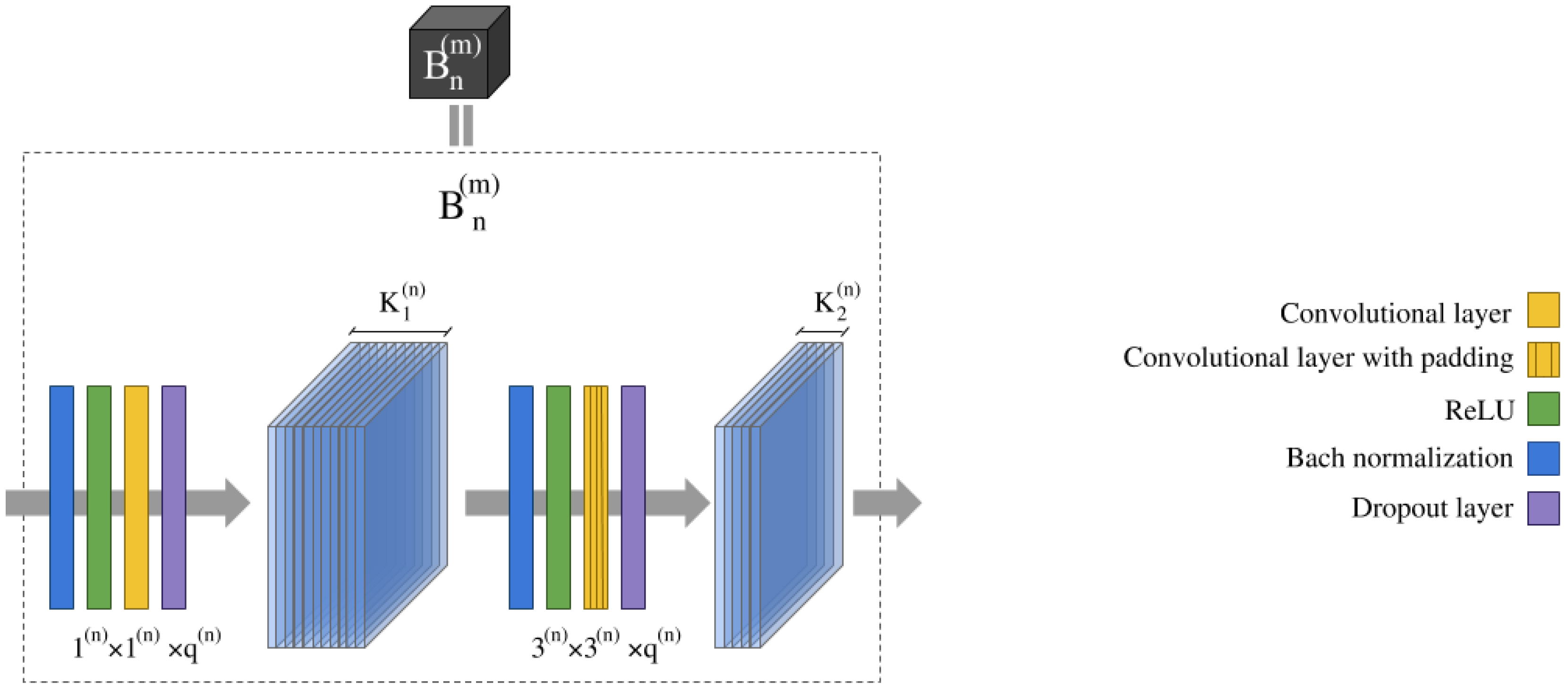
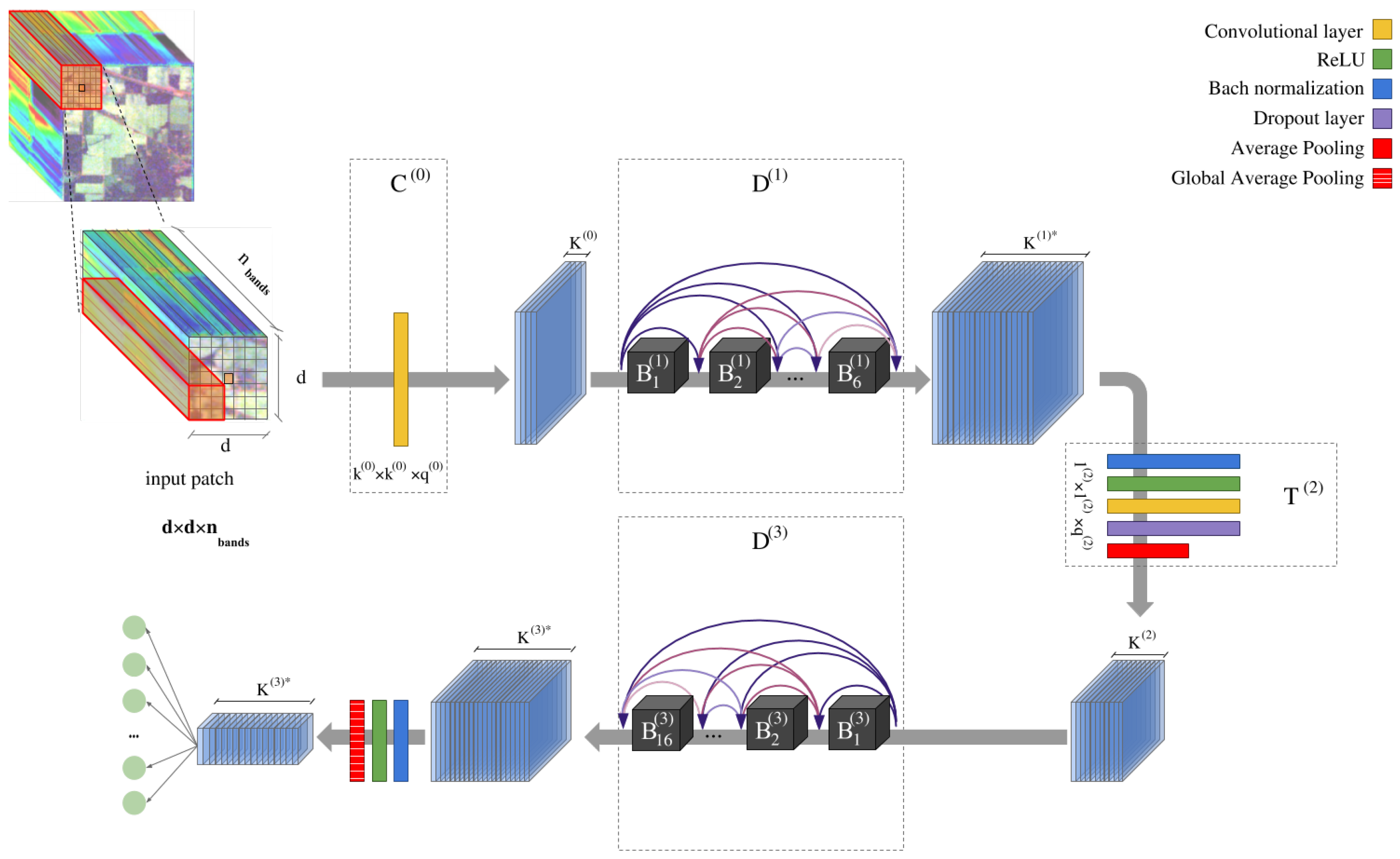
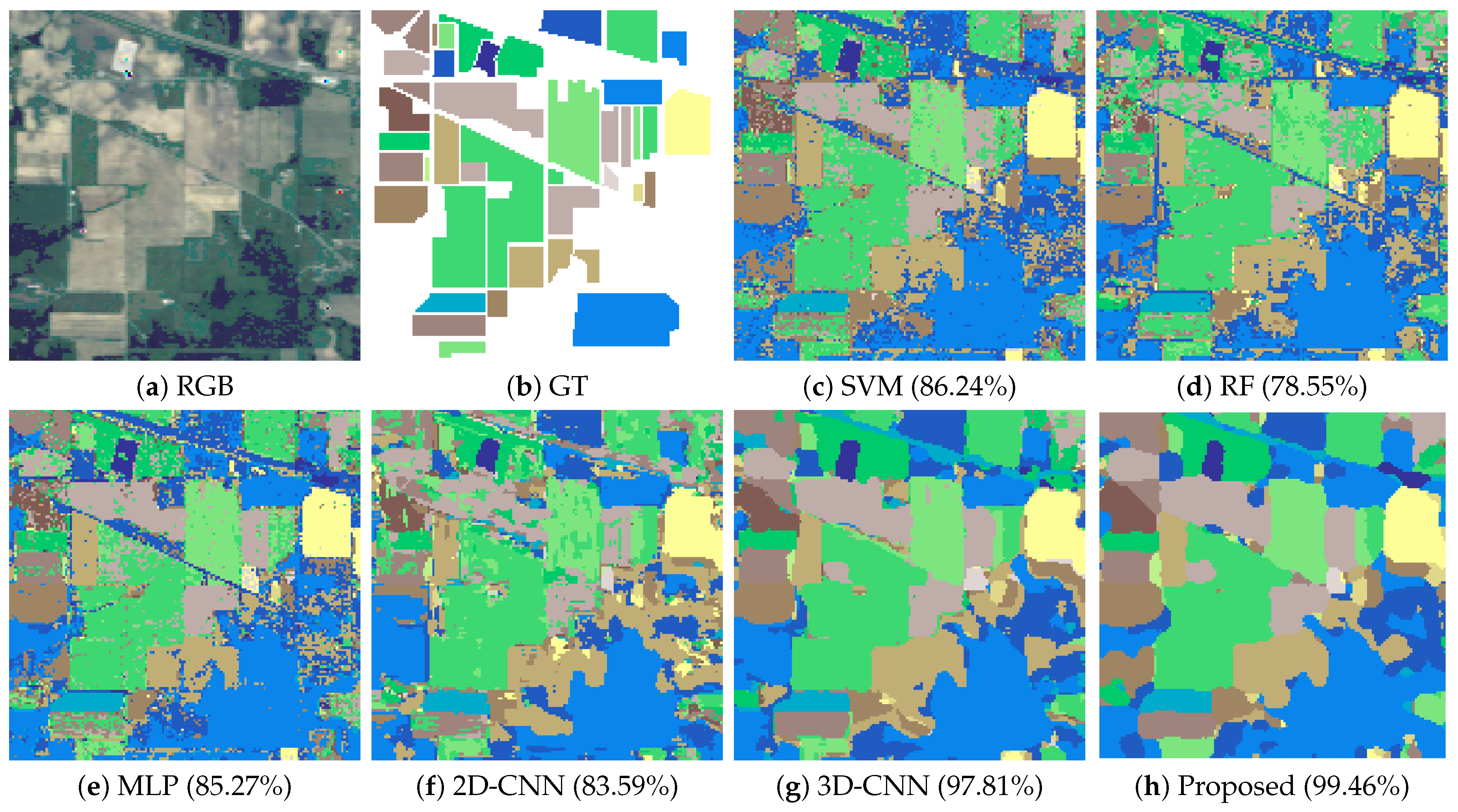
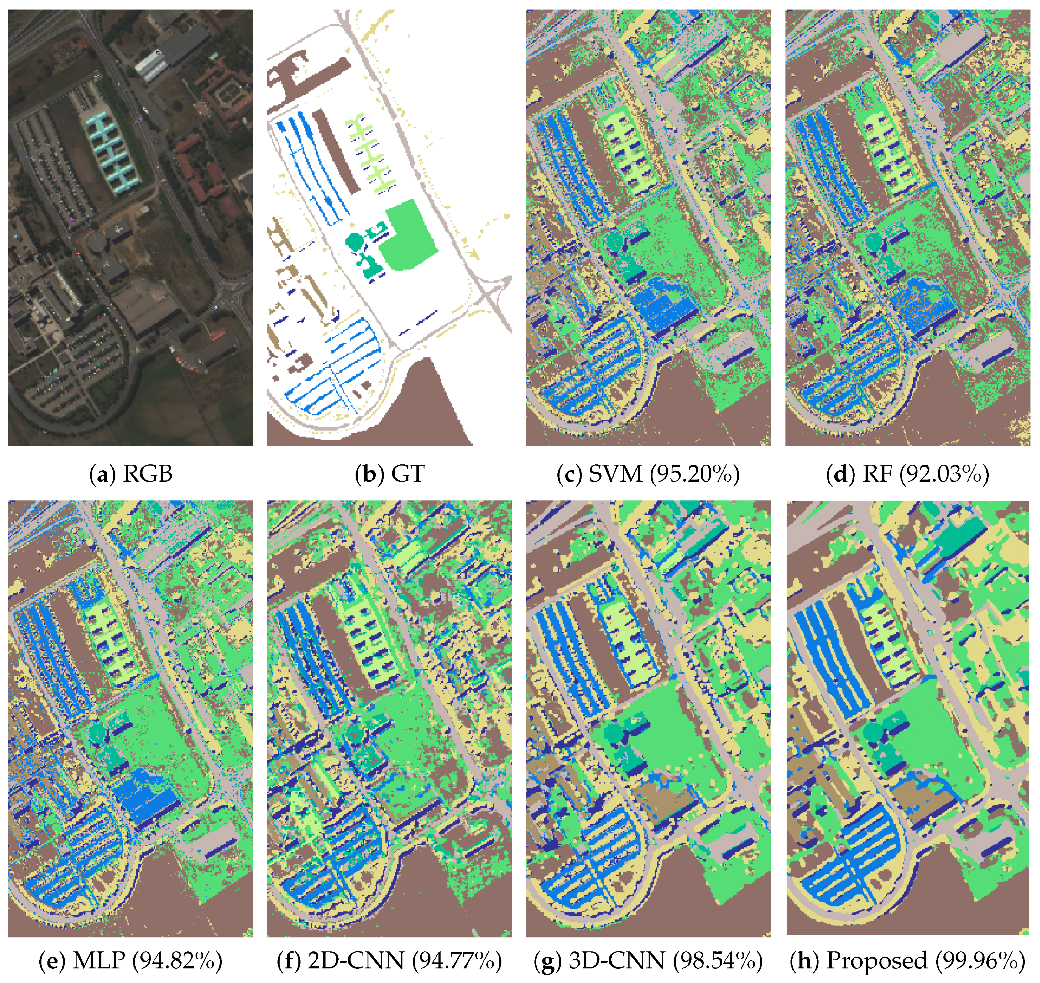
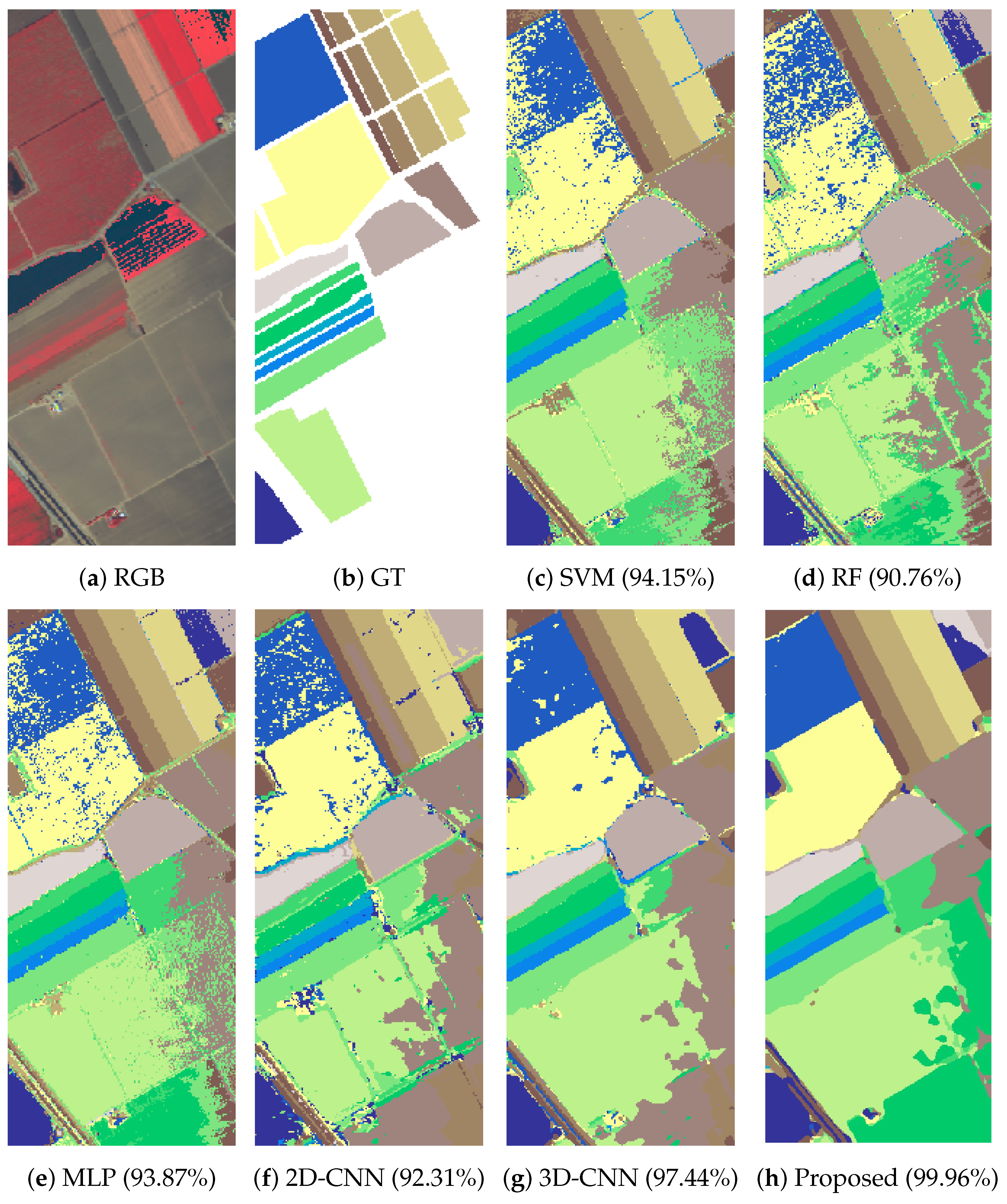
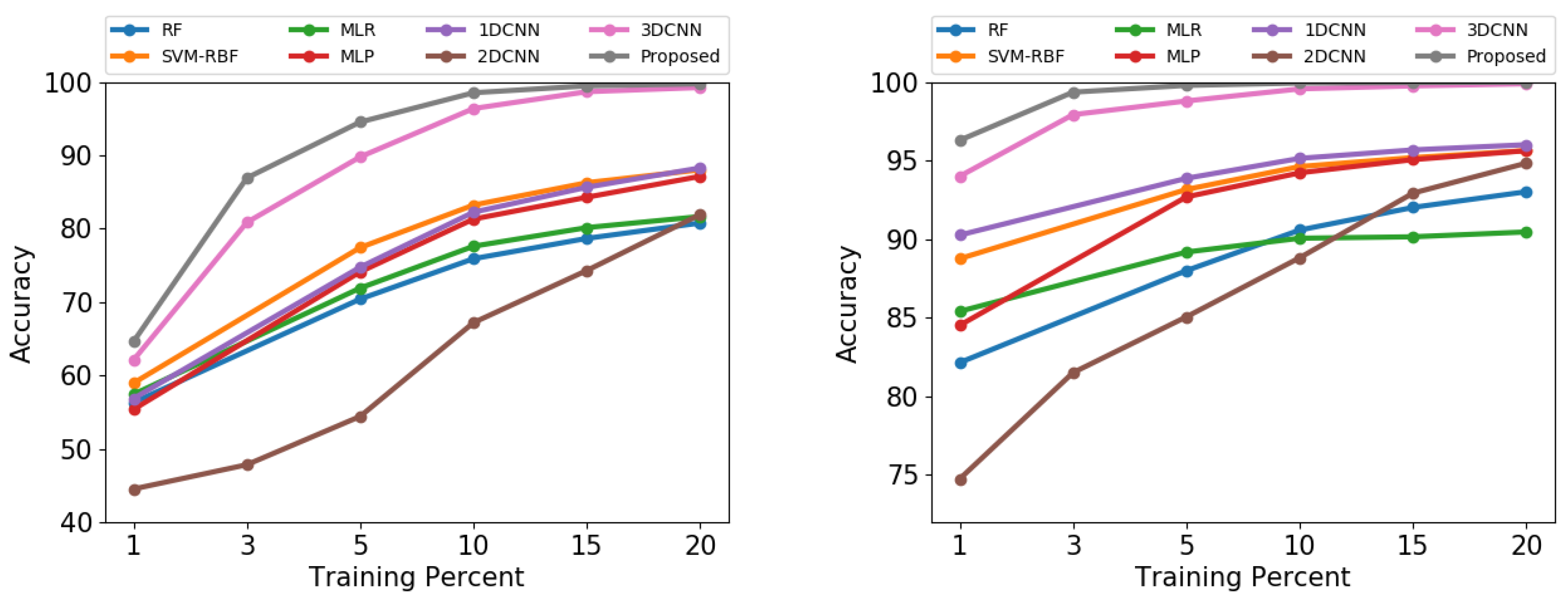
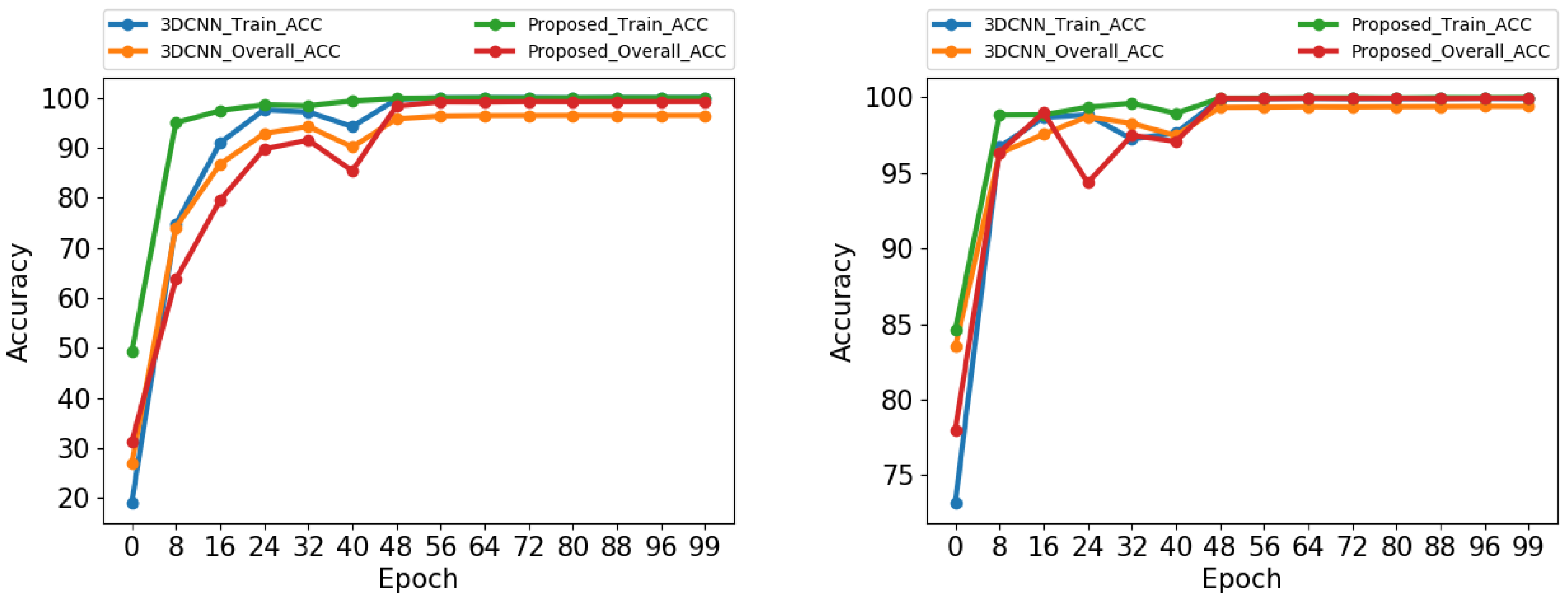
Table 1.
Parameters used in the different layers of the proposed network topology. Kernels are indicated as , while strides are represented by s. The growth rate has been fixed to , with .
Table 1.
Parameters used in the different layers of the proposed network topology. Kernels are indicated as , while strides are represented by s. The growth rate has been fixed to , with .
| Input Convolutional Layer | |
| kernels = , | |
| First dense block | |
| kernels = with , , ReLU, dropout = | |
| Transition layer | |
| kernels = , with , , ReLU, dropout = | |
| Average Pooling , | |
| Second dense block | |
| kernels = with , , ReLU, dropout = | |
| Classification layers | |
| ReLU, Global Average Pooling with output , with | |
| Fully connected of layers, with softmax | |
Table 2.
Number of samples of the Indian Pines (IP), University of Pavia (UP), Salinas Valley (SV) and Kennedy Space Center (KSC) hyperspectral datasets.
Table 2.
Number of samples of the Indian Pines (IP), University of Pavia (UP), Salinas Valley (SV) and Kennedy Space Center (KSC) hyperspectral datasets.

Table 3.
Classification results for the Indian Pines (IP) dataset using of the labeled data for training and input spatial patch size.
Table 3.
Classification results for the Indian Pines (IP) dataset using of the labeled data for training and input spatial patch size.
| Class | SVM | RF | MLP | 2D-CNN | 3D-CNN | Proposed |
|---|---|---|---|---|---|---|
| 1 | 68.04 ± 6.95 | 33.04 ± 7.45 | 62.39 ± 13.96 | 65.87 ± 10.34 | 89.13 ± 7.28 | 93.91 ± 4.64 |
| 2 | 83.55 ± 1.31 | 66.68 ± 1.67 | 83.84 ± 2.46 | 81.04 ± 3.28 | 98.33 ± 0.71 | 99.38 ± 0.44 |
| 3 | 73.82 ± 1.44 | 56.20 ± 2.41 | 76.37 ± 5.03 | 79.07 ± 6.75 | 98.05 ± 1.40 | 99.4 ± 0.31 |
| 4 | 71.98 ± 3.86 | 41.10 ± 2.50 | 68.35 ± 6.12 | 82.70 ± 8.34 | 98.23 ± 0.62 | 99.49 ± 0.62 |
| 5 | 94.29 ± 0.97 | 87.12 ± 1.73 | 90.87 ± 2.09 | 69.25 ± 10.58 | 97.56 ± 2.84 | 98.84 ± 0.59 |
| 6 | 97.32 ± 0.97 | 95.32 ± 1.79 | 96.95 ± 1.10 | 88.29 ± 5.51 | 98.93 ± 1.14 | 99.84 ± 0.16 |
| 7 | 88.21 ± 5.06 | 32.86 ± 12.66 | 78.21 ± 10.28 | 67.86 ± 25.65 | 83.57 ± 19.51 | 99.29 ± 1.43 |
| 8 | 98.16 ± 0.75 | 98.49 ± 0.81 | 98.08 ± 0.90 | 96.26 ± 1.60 | 99.41 ± 0.61 | 99.96 ± 0.08 |
| 9 | 52.00 ± 8.43 | 13.00 ± 3.32 | 72.00 ± 8.12 | 67.00 ± 27.68 | 65.00 ± 21.68 | 100.0 ± 0.0 |
| 10 | 79.49 ± 2.76 | 69.95 ± 4.31 | 82.17 ± 5.41 | 68.82 ± 9.80 | 97.22 ± 0.31 | 99.36 ± 0.35 |
| 11 | 86.83 ± 1.05 | 90.66 ± 1.18 | 83.66 ± 2.85 | 86.55 ± 3.14 | 98.12 ± 2.16 | 99.47 ± 0.29 |
| 12 | 83.41 ± 2.26 | 55.43 ± 4.80 | 75.89 ± 3.33 | 73.41 ± 6.07 | 93.09 ± 5.85 | 99.33 ± 0.44 |
| 13 | 97.41 ± 2.99 | 93.32 ± 2.04 | 98.68 ± 0.54 | 94.54 ± 4.80 | 99.80 ± 0.39 | 100.0 ± 0.0 |
| 14 | 96.14 ± 0.97 | 96.45 ± 0.76 | 96.17 ± 1.02 | 96.24 ± 2.33 | 99.43 ± 0.33 | 99.76 ± 0.34 |
| 15 | 67.31 ± 3.05 | 50.44 ± 2.44 | 67.80 ± 3.56 | 85.39 ± 7.71 | 96.58 ± 2.81 | 99.17 ± 0.72 |
| 16 | 92.47 ± 4.14 | 85.27 ± 3.37 | 88.71 ± 2.77 | 92.90 ± 3.97 | 93.12 ± 3.82 | 98.49 ± 1.1 |
| OA (%) | 86.24 ± 0.38 | 78.55 ± 0.68 | 85.27 ± 0.47 | 83.59 ± 0.88 | 97.81 ± 0.56 | 99.46 ± 0.07 |
| AA (%) | 83.15 ± 1.10 | 66.58 ± 0.93 | 82.51 ± 1.04 | 80.95 ± 1.55 | 94.10 ± 2.00 | 99.11 ± 0.26 |
| Kappa | 84.27 ± 0.45 | 75.20 ± 0.81 | 83.20 ± 0.53 | 81.23 ± 1.04 | 97.50 ± 0.64 | 99.38 ± 0.08 |
| Time(s) | 208.98 ± 1.70 | 1301.68 ± 45.94 | 7.31 ± 0.15 | 56.45 ± 0.19 | 39.62 ± 0.67 | 160.60 ± 1.68 |
Table 4.
Classification results for the University of Pavia (UP) dataset using of the labeled data for training and input spatial size.
Table 4.
Classification results for the University of Pavia (UP) dataset using of the labeled data for training and input spatial size.
| Class | SVM | RF | MLP | 2D-CNN | 3D-CNN | Proposed |
|---|---|---|---|---|---|---|
| 1 | 95.36 ± 0.30 | 93.52 ± 0.45 | 94.17 ± 1.73 | 93.43 ± 2.70 | 99.16 ± 0.25 | 99.95 ± 0.06 |
| 2 | 98.25 ± 0.16 | 98.29 ± 0.18 | 98.06 ± 0.50 | 97.59 ± 0.88 | 99.77 ± 0.17 | 99.99 ± 0.02 |
| 3 | 82.93 ± 0.91 | 75.56 ± 1.86 | 79.27 ± 7.04 | 89.96 ± 3.30 | 96.95 ± 1.78 | 99.74 ± 0.35 |
| 4 | 95.93 ± 0.70 | 91.68 ± 0.63 | 94.61 ± 2.58 | 94.16 ± 3.24 | 98.80 ± 0.69 | 99.83 ± 0.12 |
| 5 | 99.46 ± 0.36 | 98.88 ± 0.49 | 99.63 ± 0.27 | 97.97 ± 2.69 | 99.90 ± 0.17 | 99.97 ± 0.06 |
| 6 | 91.76 ± 0.60 | 74.54 ± 0.97 | 93.60 ± 1.70 | 89.62 ± 4.10 | 99.88 ± 0.12 | 100.0 ± 0.0 |
| 7 | 88.59 ± 0.65 | 81.01 ± 1.74 | 88.53 ± 3.47 | 80.20 ± 4.82 | 96.54 ± 1.41 | 99.95 ± 0.06 |
| 8 | 90.14 ± 0.54 | 90.70 ± 0.75 | 89.59 ± 4.56 | 96.05 ± 1.88 | 98.56 ± 0.78 | 99.99 ± 0.01 |
| 9 | 99.97 ± 0.05 | 99.75 ± 0.26 | 99.63 ± 0.28 | 99.48 ± 0.27 | 99.79 ± 0.19 | 99.89 ± 0.16 |
| OA (%) | 95.20 ± 0.13 | 92.03 ± 0.21 | 94.82 ± 0.26 | 94.77 ± 0.72 | 99.28 ± 0.25 | 99.96 ± 0.03 |
| AA (%) | 93.60 ± 0.14 | 89.33 ± 0.33 | 93.01 ± 0.60 | 93.16 ± 1.23 | 98.81 ± 0.33 | 99.93 ± 0.07 |
| Kappa | 93.63 ± 0.17 | 89.30 ± 0.28 | 93.13 ± 0.34 | 93.05 ± 0.97 | 99.04 ± 0.32 | 99.94 ± 0.04 |
| Time(s) | 6084.92 ± 55.64 | 6188.75 ± 35.16 | 29.10 ± 0.92 | 172.29 ± 0.71 | 140.09 ± 1.63 | 544.59 ± 4.57 |
Table 5.
Classification results for the Salinas Valley (SV) dataset using of the labeled data for training and input spatial patch size.
Table 5.
Classification results for the Salinas Valley (SV) dataset using of the labeled data for training and input spatial patch size.
| Class | SVM | RF | MLP | 2D-CNN | 3D-CNN | Proposed |
|---|---|---|---|---|---|---|
| 1 | 99.68 ± 0.21 | 99.61 ± 0.12 | 99.72 ± 0.42 | 87.99 ± 17.62 | 100.00 ± 0.00 | 100.00 ± 0.0 |
| 2 | 99.87 ± 0.12 | 99.86 ± 0.07 | 99.88 ± 0.15 | 99.75 ± 0.23 | 99.99 ± 0.01 | 100.00 ± 0.0 |
| 3 | 99.74 ± 0.11 | 99.22 ± 0.51 | 99.43 ± 0.44 | 81.40 ± 10.85 | 99.94 ± 0.07 | 100.00 ± 0.0 |
| 4 | 99.48 ± 0.18 | 99.28 ± 0.44 | 99.61 ± 0.27 | 95.11 ± 5.51 | 99.83 ± 0.23 | 99.97 ± 0.06 |
| 5 | 99.24 ± 0.31 | 98.46 ± 0.21 | 99.25 ± 0.48 | 64.31 ± 12.09 | 99.90 ± 0.09 | 99.97 ± 0.06 |
| 6 | 99.92 ± 0.06 | 99.80 ± 0.09 | 99.92 ± 0.07 | 99.60 ± 0.11 | 100.00 ± 0.00 | 100.00 ± 0.0 |
| 7 | 99.70 ± 0.15 | 99.58 ± 0.09 | 99.82 ± 0.12 | 98.01 ± 4.54 | 99.90 ± 0.15 | 100.00 ± 0.0 |
| 8 | 90.87 ± 0.39 | 84.41 ± 1.34 | 85.41 ± 8.00 | 91.89 ± 2.44 | 90.67 ± 6.83 | 99.92 ± 0.1 |
| 9 | 99.94 ± 0.02 | 99.07 ± 0.17 | 99.86 ± 0.07 | 98.02 ± 1.56 | 99.99 ± 0.01 | 100.00 ± 0.0 |
| 10 | 98.26 ± 0.27 | 93.40 ± 0.58 | 97.15 ± 0.77 | 97.05 ± 0.67 | 99.27 ± 0.43 | 99.99 ± 0.01 |
| 11 | 99.61 ± 0.34 | 94.79 ± 0.59 | 97.42 ± 2.29 | 94.58 ± 3.59 | 99.48 ± 0.73 | 99.91 ± 0.19 |
| 12 | 99.93 ± 0.05 | 99.08 ± 0.29 | 99.80 ± 0.14 | 92.67 ± 5.75 | 99.76 ± 0.38 | 100.00 ± 0.0 |
| 13 | 99.07 ± 0.72 | 98.23 ± 0.69 | 99.40 ± 0.28 | 98.10 ± 0.76 | 99.63 ± 0.58 | 100.00 ± 0.0 |
| 14 | 98.08 ± 1.00 | 92.81 ± 1.04 | 97.58 ± 0.94 | 95.25 ± 5.74 | 99.94 ± 0.11 | 100.00 ± 0.0 |
| 15 | 72.83 ± 0.78 | 63.32 ± 1.82 | 80.27 ± 8.41 | 87.36 ± 3.87 | 96.18 ± 1.52 | 99.94 ± 0.05 |
| 16 | 99.45 ± 0.25 | 98.17 ± 0.36 | 98.97 ± 0.38 | 93.72 ± 1.66 | 99.39 ± 0.42 | 99.75 ± 0.4 |
| OA (%) | 94.15 ± 0.10 | 90.76 ± 0.24 | 93.87 ± 0.70 | 92.31 ± 1.62 | 97.44 ± 1.28 | 99.96 ± 0.03 |
| AA (%) | 97.23 ± 0.11 | 94.94 ± 0.12 | 97.09 ± 0.33 | 92.18 ± 2.72 | 98.99 ± 0.40 | 99.97 ± 0.05 |
| Kappa | 93.48 ± 0.11 | 89.70 ± 0.26 | 93.18 ± 0.77 | 91.43 ± 1.81 | 97.15 ± 1.42 | 99.96 ± 0.03 |
| Time(s) | 3110.30 ± 29.20 | 4694.29 ± 158.39 | 36.42 ± 0.11 | 296.62 ± 3.52 | 260.41 ± 6.09 | 742.09 ± 8.22 |
Table 6.
Classification results obtained for the IP dataset using the DFCNN model in Paoletti et al. [71], with patch sizes of and , and the proposed model, with the smallest patch size of .
Table 6.
Classification results obtained for the IP dataset using the DFCNN model in Paoletti et al. [71], with patch sizes of and , and the proposed model, with the smallest patch size of .
| Classes | Samples | d = 9 | d = 19 | d = 29 | Proposed d = 9 | |
|---|---|---|---|---|---|---|
| 1 | Alfalfa | 30 | 100.00 | 100.00 | 100.00 | 100.00 |
| 2 | Corn-notill | 150 | 90.57 | 94.06 | 97.17 | 98.24 |
| 3 | Corn-min | 150 | 97.69 | 96.43 | 98.17 | 99.37 |
| 4 | Corn | 100 | 99.92 | 100.00 | 100.00 | 100.00 |
| 5 | Grass/Pasture | 150 | 98.10 | 98.72 | 98.76 | 99.67 |
| 6 | Grass/Trees | 150 | 99.34 | 99.67 | 100.00 | 99.73 |
| 7 | Grass/pasture-mowed | 20 | 100.00 | 100.00 | 100.00 | 100.00 |
| 8 | Hay-windrowed | 150 | 99.58 | 99.92 | 100.00 | 100.00 |
| 9 | Oats | 15 | 100.00 | 100.00 | 100.00 | 100.00 |
| 10 | Soybeans-notill | 150 | 94.28 | 97.63 | 99.14 | 99.65 |
| 11 | Soybeans-min | 150 | 87.75 | 92.93 | 94.59 | 96.89 |
| 12 | Soybean-clean | 150 | 94.81 | 97.17 | 99.06 | 99.53 |
| 13 | Wheat | 150 | 100.00 | 100.00 | 100.00 | 100.00 |
| 14 | Woods | 150 | 98.09 | 97.88 | 99.76 | 98.85 |
| 15 | Bldg-Grass-Tree-Drives | 50 | 89.79 | 95.80 | 98.39 | 98.24 |
| 16 | Stone-steel towers | 50 | 100.00 | 99.57 | 98.92 | 99.57 |
| Overall Accuracy (OA) | 93.94 | 96.29 | 97.87 | 98.65 | ||
| Average Accuracy (AA) | 96.87 | 98.11 | 99.00 | 99.36 | ||
| Kappa | 93.12 | 95.78 | 97.57 | 98.46 | ||
| Runtime (s) | 74.47 | 189.51 | 158.42 | 132.04 | ||
Table 7.
Classification results obtained for the UP dataset using the DFCNN model in Paoletti et al. [71], with patch sizes of and , and the proposed model, with the smallest patch size of .
Table 7.
Classification results obtained for the UP dataset using the DFCNN model in Paoletti et al. [71], with patch sizes of and , and the proposed model, with the smallest patch size of .
| Classes | Samples | d = 15 | d = 21 | d = 23 | Proposed d = 15 | |
|---|---|---|---|---|---|---|
| 1 | Asphalt | 548 | 97.53 | 98.80 | 98.59 | 99.97 |
| 2 | Meadows | 540 | 98.98 | 99.46 | 99.60 | 99.96 |
| 3 | Gravel | 392 | 98.96 | 99.59 | 99.45 | 100.00 |
| 4 | Trees | 542 | 99.75 | 99.68 | 99.57 | 99.75 |
| 5 | Painted metal sheets | 256 | 99.93 | 99.78 | 99.61 | 99.94 |
| 6 | Bare Soil | 532 | 99.42 | 99.93 | 99.84 | 100.00 |
| 7 | Bitumen | 375 | 98.71 | 99.88 | 100.00 | 100.00 |
| 8 | Self-Blocking Bricks | 514 | 98.58 | 99.53 | 99.67 | 99.99 |
| 9 | Shadows | 231 | 99.87 | 99.79 | 99.83 | 100.00 |
| Overall Accuracy (OA) | 98.87 | 99.47 | 99.48 | 99.96 | ||
| Average Accuracy (AA) | 99.08 | 99.60 | 99.57 | 99.96 | ||
| Kappa | 98.51 | 99.30 | 99.32 | 99.94 | ||
| Runtime (s) | 43.16 | 94.57 | 107.56 | 519.09 | ||
Table 8.
Overall Accuracy (%) achieved by the SSRN method [119] and the proposed approach when considering different input spatial patch sizes.
Table 8.
Overall Accuracy (%) achieved by the SSRN method [119] and the proposed approach when considering different input spatial patch sizes.
| Spatial Size | Indian Pines (IP) | Kennedy Space Center (KSC) | University of Pavia (UP) | |||
|---|---|---|---|---|---|---|
| SSRN [119] | Proposed | SSRN [119] | Proposed | SSRN [119] | Proposed | |
| 5×5 | 92.83 (0.66) | 97.85 (0.28) | 96.99 (0.55) | 97.11 (0.48) | 98.72 (0.17) | 99.13 (0.08) |
| 7×7 | 97.81 (0.34) | 99.24 (0.14) | 99.01 (0.31) | 98.81 (0.23) | 99.54 (0.11) | 99.71 (0.10) |
| 9×9 | 98.68 (0.29) | 99.58 (0.09) | 99.51 (0.25) | 99.52 (0.19) | 99.73 (0.15) | 99.82 (0.07) |
| 11×11 | 98.70 (0.21) | 99.74 (0.08) | 99.57 (0.54) | 99.73 (0.15) | 99.79 (0.08) | 99.93 (0.03) |
© 2018 by the authors. Licensee MDPI, Basel, Switzerland. This article is an open access article distributed under the terms and conditions of the Creative Commons Attribution (CC BY) license (http://creativecommons.org/licenses/by/4.0/).
Share and Cite
MDPI and ACS Style
Paoletti, M.E.; Haut, J.M.; Plaza, J.; Plaza, A. Deep&Dense Convolutional Neural Network for Hyperspectral Image Classification. Remote Sens. 2018, 10, 1454. https://doi.org/10.3390/rs10091454
AMA Style
Paoletti ME, Haut JM, Plaza J, Plaza A. Deep&Dense Convolutional Neural Network for Hyperspectral Image Classification. Remote Sensing. 2018; 10(9):1454. https://doi.org/10.3390/rs10091454
Chicago/Turabian StylePaoletti, Mercedes E., Juan M. Haut, Javier Plaza, and Antonio Plaza. 2018. "Deep&Dense Convolutional Neural Network for Hyperspectral Image Classification" Remote Sensing 10, no. 9: 1454. https://doi.org/10.3390/rs10091454
Note that from the first issue of 2016, this journal uses article numbers instead of page numbers. See further details here.