Supervised Classification of Multisensor Remotely Sensed Images Using a Deep Learning Framework
by
Sankaranarayanan Piramanayagam
1,*, 
Eli Saber
1,2,
Wade Schwartzkopf
3,† and
Frederick W. Koehler
3 1
Chester F. Carlson Center for Imaging Science, Rochester Institute of Technology, 54 Lomb Memorial Drive, Rochester, NY 14623, USA
2
Department of Electrical & Microelectronic Engineering, Rochester Institute of Technology, 54 Lomb Memorial Drive, Rochester, NY 14623, USA
3
National Geospatial-Intelligence Agency, 7500 GEOINT Dr, Springfield, VA 22153, USA
*
Author to whom correspondence should be addressed.
†
NGA Contractor.
Remote Sens. 2018, 10(9), 1429; https://doi.org/10.3390/rs10091429
Submission received: 2 July 2018
/
Revised: 30 August 2018
/
Accepted: 31 August 2018
/
Published: 7 September 2018
(This article belongs to the Special Issue Recent Advances in Neural Networks for Remote Sensing)
Abstract
:In this paper, we present a convolutional neural network (CNN)-based method to efficiently combine information from multisensor remotely sensed images for pixel-wise semantic classification. The CNN features obtained from multiple spectral bands are fused at the initial layers of deep neural networks as opposed to final layers. The early fusion architecture has fewer parameters and thereby reduces the computational time and GPU memory during training and inference. We also propose a composite fusion architecture that fuses features throughout the network. The methods were validated on four different datasets: ISPRS Potsdam, Vaihingen, IEEE Zeebruges and Sentinel-1, Sentinel-2 dataset. For the Sentinel-1,-2 datasets, we obtain the ground truth labels for three classes from OpenStreetMap. Results on all the images show early fusion, specifically after layer three of the network, achieves results similar to or better than a decision level fusion mechanism. The performance of the proposed architecture is also on par with the state-of-the-art results.
1. Introduction
Semantic classification of aerial/satellite images is essential for land cover and land use mapping, change detection, emergency response or management, and various other applications [1]. Numerous pixel- and object-based approaches, such as support vector machine (SVM) [2], random forest [3], and others [1], have been proposed to classify these images. These methods typically involve a feature generation and selection step before the classification stage. The intermediate step allows for selecting minimal but highly discriminative features. Reducing the number of features also avoids overfitting issues that often occur in remote sensing image classification, especially in hyperspectral images [4], where high dimensional data is available with limited ground truth data. Given this, extensive research has been conducted to select appropriate features and classifiers for various classification scenarios. New methods [5,6] are also being actively proposed. On the other hand, recent deep learning methods learn features automatically from the training data and have been successfully applied to various computer vision tasks with improved performance. This was made possible by improvements in neural network design, vast training datasets, and fast computation through graphical processing units (GPUs). The networks are trained in either a supervised or unsupervised fashion. In the supervised method, large input data and corresponding ground truth data are used to train the deep neural networks. Imagenet [7] is one such large dataset, and VGG-16 [8] is a convolutional network that uses the dataset for image classification. In our work, we extend the supervised deep learning methods for multisensor aerial/satellite image pixel-wise classification. The neural network framework learns the complex relationships between the input and ground truth data and generates results in the form of test data. The performance is significantly better than prior methods like SVM or random forest.
In this paper, we investigate an optimal way to combine features from multisensor imagery in a neural network framework [9]. Multiple convolutional neural network (CNN) branches were used to generate and fuse features of the multisensor data and perform semantic classification. The dataset used in the paper includes ISPRS Potsdam, Vaihingen, Sentinel-1, Sentinel-2, and IEEE Zeebruges datasets [10,11,12,13]. The Potsdam dataset makes available four bands, IR, R, G, B, and an additional normalized digital surface model (NDSM). These channels can be input to the neural networks in numerous ways. We employ CNN architectures (specifically, fully convolutional neural network (FCN) by Shelhamer et al. [14] and segmentation network (SegNet) by Badrinarayanan et al. [15]) on groups of these bands, e.g., one set of convolutional layers for R, G, B bands and another set for IR, NDVI, NDSM. Features from these branches are then merged at the initial and later stages of the network. We compare the results from early fusion, late fusion, and a third composite fusion, where features are merged throughout the network. Results from the three datasets indicate both late and early fusion methods achieve similar performance. Hence, it is desirable to combine features at early layers of CNN for a given multisensor image. Given our work, the main contributions of the paper include the following:
- Fuse information from multi-sensor images at various layers of deep neural networks and compare the results to find the optimal configuration. An example includes, combining RGB and LiDAR features obtained from distinct branches of FCN at various layers of the network. Fusion of features in early stages of neural networks, FCN and SegNet, achieve results similar to late fusion but with less GPU memory and reduced run time.
- Propose a composite fusion architecture that combines information from multi-sensor images throughout the network.
- Efficiently fuse multi-sensor data in neural network architecture and benchmark the proposed methods on various datasets. The datasets include (a) Sentinel-1 and -2 data (SAR and Multispectral), (b) ISPRS and IEEE datasets (Optical and LiDAR data). OpenStreetMap were used for generating ground truth data for Sentinel-1 and -2 satellite images. The performance of these proposed architectures are on par with the state-of-the-art results.
2. Literature Review
In the literature, many methods have been proposed to classify multisensor images. In this section, we first discuss the different fusion mechanisms and methods that combine information from multisensor data. We then proceed to examine the methods that combine multisensor information in a deep learning framework. Since it relates directly to our proposed work, we briefly describe all the recent approaches that yield state-of-the-art classification results. Finally, we review the general deep learning-based methods that classify aerial/satellite images.
2.1. Multisensor Fusion
Fusion of remotely sensed data acquired from multiple sensors for image classification has been a widely researched field [1,16,17,18,19,20]. The fusion techniques can be broadly categorized [1] into feature, decision, and pixel-/subpixel-level fusion and ensembles of these methods. Our current work falls into the categories of feature- and decision-level fusion. In decision-level fusion [19], the data are sent to different classifiers and the individual results are merged to obtain the final map. Feature-level fusion involves selecting features from multiple modalities and effectively combining them before a classification step.
In terms of the modalities, extensive research has been conducted to combine optical images with synthetic aperture radar (SAR) and LiDAR data. Since SAR images are acquired by an active sensor and the wavelength used could penetrate cloud cover, data can be obtained in any weather [21]. This allows SAR images to be used along with high-resolution optical data acquired at an earlier time for disaster management, urban expansion, and other applications [22,23,24]. In an early work, Waske et al. [25] first classified multitemporal SAR and multispectral Thematic Mapper (TM) images and their segmentation at different levels using a support vector machine (SVM). The individual predictions were then stacked and passed to another SVM and random forest classifier to obtain final land-cover maps. The use of multilevel and multisource data in the framework provided robust results. In a more recent study [26], 12 TM images and 25 SAR images captured over a period of time were combined using a spatiotemporal fuzzy clustering method to classify changed/unchanged pixels. With the availability of Sentinel-1 (SAR) and Sentinel-2 (multispectral) data, pixel-based [27] and object-based [28] methods have been proposed to combine them for land-cover classification. Similarly, optical images have been fused with LiDAR data for various applications, which include building extraction [29,30], semantic segmentation of forest stands [31], and others. An IEEE GRSS data fusion contest [32,33] is held every year, and new multisensor datasets like ISPRS Potsdam and Vaihingen [11] have accelerated research in the field.
2.2. Deep Learning: Multistream Fusion Architecture
Deep learning methods that fuse information from different modalities were initially proposed in the computer vision community [34,35]. Karpathy et al. [34] proposed several approaches to fuse spatial and temporal information available on video for large-scale video classification tasks. They used multiple frames in early, late, and slow fusion frameworks to predict various actions like cycling, bowling, etc., that occur in input video. They reported that slow fusion has robust performance, and in the future, they will test the framework on broader video categories. Another two-stream neural network was proposed by Simonyan et al. [35] to combine spatial and temporal information for action recognition. In their work, a single frame of video was input to the spatial stream of VGG-16 network [8] and multi-frame optical flow images were passed to the second VGG-16 network. The results from both branches were combined at the end for video classification. They report competitive performance and indicate that results could be further improved with additional training for the temporal branch.
In our initial work [9], we investigated the application of neural networks for multisensor aerial image classification. We merged the features before the first fully convolutional layer of FCN-8 architecture (instead of decision-level fusion). The features from two branches were concatenated and sent as input to a convolutional layer. The intuition was that an additional convolution layer would learn to select the features from both branches that are optimal for pixel-wise classification. We found that results obtained were similar to the decision-level fusion on the aerial image dataset and led to the current thorough analysis. Feichtenhofer et al. [36], around the same period, proposed a two-stream fusion architecture to combine single-frame and corresponding optical-flow images for the action recognition task. Their method was able to find better pixel correspondence between the spatial and temporal streams/branches. They did extensive experiments to combine features from multiple streams through sum, max, convolution, and bilateral operations and reported that sum and convolution strategies produced the best results. Another fusion architecture, named FuseNet [37], which sums the features at every convolutional layer, was proposed to combine RGB and depth information for semantic classification. Recently, Audebert et al. [38] proposed an efficient multiscale approach for the semantic classification of multimodal high-resolution remotely sensed data (ISPRS data). They compared results between the FuseNet method and a late fusion approach with residual correction. In these methods, feature information is obtained from two or more streams and later merged at some layer of the network. These fused features are then used to generate the final classification result. Most often the individual streams use pre-trained weights from another domain to generate features. It is possible, for the given task, features generated could be redundant or not optimized.
2.3. Deep Learning: Semantic Classification
Over the past few years, numerous CNN-based methods [39] have been proposed to assign a label for each pixel of an image or video. FCN, proposed by Shelhamer et al. [14], was the first method to train a network end-to-end for semantic segmentation. One of the limitations of the method was that it had millions of trainable parameters. Badrinarayanan et al. [15], in their work, reduced the number of parameters and proposed a new encoder-decoder architecture called SegNet. This significantly reduced the network memory while achieving performance similar to the FCN method. Another architecture, ResNet [40], has been augmented with conditional random fields [41] to further improve the semantic segmentation performance. These methods have been applied to multimodal data: RGB images [14,15,40], video [42], RGB + depth images [43], and others.
Deep learning methods for semantic segmentation are being actively applied to aerial images for land-use classification. Paisitkriangkrai et al. [44] proposed a method that combines classification results obtained from manually extracted and CNN features. Initially, two sets of features were generated from an image patch: (a) features like NDVI, edges, saturation, etc., and (b) CNN features. These features were then passed through two separate classifiers to obtain per-pixel probability maps. A CRF-based method further processes the ensemble of the maps to generate the final result. The performance of the method is better than stand-alone CNN methods. Sherrah [45] proposed a no-downsampling FCN approach that used sparse filters for classification. The method was tested on the Potsdam and Vaihingen datasets by employing two networks: FCN for color infrared (CIR) data and no-downsampling FCN for DSM data. Even though training time increased because of the no-downsampling operation, the method generated accurate and dense results for these high-resolution images. In another work [46], CNN predictions from CIR data and logistic regression classifier predictions from CIR and DSM data (manually extracted features) were combined within a higher-order CRF framework. The method has a simple architecture and incorporates object-level contextual information. However, the classification output is sensitive to the scale of initial segments used in higher-order terms of the CRF model. Other recent works include downsampling–upsampling CNN architecture [47] to obtain dense prediction and a patch-based CNN [48] to extract roads and buildings in urban areas. With the availability of aerial/satellite images and corresponding dense ground truth, like ISPRS [10,11], IEEE datasets [12,13], and SpaceNet challenge [49], numerous methods are being actively proposed and evaluated on these datasets.
3. Methodology
This section describes the deep learning architecture and different fusion networks proposed for combining information from multi-sensor images for pixel-wise classification.
3.1. Deep Learning Architecture
The building block of an artificial neural network is the neuron, where a weighted sum of the inputs followed by a nonlinear operation is computed. In a convolutional neural network (CNN), where the input is an image of size (e.g., 3D input for (R, G, B) images), these neurons are arranged in 3 dimensions. Each neuron is connected to only a certain number of inputs in the previous layer. Also, the weights are shared within each channel of the 3D neuron volume [50]. Let of size and of size be the input and output of a convolution layer, respectively. Output at location () is obtained from the input as follows:
Here, is the weight matrix of size with k determining the filter/kernel width, and is the bias vector of size t. For example, in a fully convolutional network (FCN) [14], the input image is of size 224 × 224 × 3 () and the first convolution layer outputs 64 (t) features of size 224 × 224. The 64 filters with support 3 × 3 × 3 (here , is of size 3 × 3 × 3 × 64 and a 64 element vector) transforms the 224 × 224 × 3 input into the 224 × 224 × 64 feature volume. The above operation (denoted as ) is followed by nonlinear activation (e.g., ReLU: ). The features obtained are further passed through multiple convolution, ReLU, and subsampling or pooling layers. These layers are then followed by a fully connected convolutional layer, where the neurons again have a 3D arrangement but each neuron has connections from all the features in the preceding layer. This transformation allows the network to generate coarse maps with spatial support. A convolution transpose layer [51] is then used to bring the coarse map to the original image resolution. The final prediction of the network is a 3-dimensional output of size . All the parameters () are learned during supervised training and then applied on new test data to classify them. There are 2 variants of the FCN architecture: FCN-32 and FCN-8. In FCN-32, the output from the scoring layer is upsampled to the original image resolution in a single step and thereby generating a coarse semantic map. Whereas in FCN-8, shown in Figure 1, gradual upsampling of scoring layer and merging of features from earlier layers are made to obtain finer semantic segmentation.
SegNet [15] is the second network used in our multimodal fusion analysis. SegNet (encoder-decoder) architecture removes the fully connected convolutional layers of the FCN and replaces them with multiple upsampling and convolution transpose layers. The downsampling information in the initial layers is also passed to a corresponding upsampling operation. These 2 modifications reduce the number of parameters of the network while achieving results comparable to FCN.
3.2. Multisensor Fusion
In general, a CNN can take an arbitrary number of spectral bands as input. Such networks, e.g., FCN or SegNet, will consist of a single stream of multiple convolutional layers. However, a large training dataset (image and corresponding ground truth data) is required to avoid overfitting. At present, only limited or moderate training datasets are available for aerial image collections. Randomly assigning values to the CNN parameters/weights and training the network from scratch with limited data will generate poor results on the test data. Thus, to avoid overfitting, the weights obtained from other tasks, like the semantic classification of RGB images, need to be used as initial values and further fine-tuned with the given labeled aerial image set. This transfer learning process [52] has been successfully used to classify aerial RGB images.
In a multisensor setup, where more than three bands are available, a simple approach is to employ two or more neural network branches and fuse the features at the very end to obtain a classification map. The parameters of the different streams could be initialized with pretrained weights from the image categorization task [14] and then further fine-tuned with current labeled data. However, the main drawback of late fusion architecture is that the number of neurons/operations is predominantly large, hence they require more computation time in both the training and testing phase. Also, this fusion approach may not provide the best results for a given dataset.
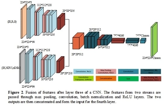
In our work, we propose a CNN that efficiently combines features from multiple spectral bands for semantic classification. The task at hand is to design a network that (a) takes in multiple bands, (b) requires minimal parameters and memory, (c) provides good quantitative results, and (d) uses pretrained weights because of moderate training data size. The proposed fusion architecture uses the existing CNN, e.g., FCN or SegNet, as a base network. The set of convolution filters that operate on features of the same scale is referred to as a layer. In FCN-8, layer 1 and layer 2 consist of two convolution filters each and layers 3 to 5 consist of three convolution filters (Figure 1). These are followed by two fully connected convolutional (FC) layers and a final scoring layer. The FC layer by itself consists of numerous parameters. Having multiple such layers in a network (e.g., late fusion) will increase the computational memory considerably. Hence, to construct a memory-efficient network, it is necessary to fuse the features before the FC layer (anywhere after layers 1 to 5). The features obtained from early layers are more general and correspond to low-level features. Yosinski et al. [52] studied the transition of features from general in shallow (early) layers of a network to specific ones for a given task in deeper layers. In one of their experiments, they found that transferring shallow-layer weights from one task to another and fine-tuning with additional new data provided results comparable to transferring deeper-layer features. Based on these findings, we anticipated that fusing pretrained features at some point before the FC layer and doing sufficient fine-tuning should provide results on par with late fusion. Similarly, for the SegNet architecture, we combined features in the early layers (encoder) of the network as opposed to the deeper layers (decoder).
The proposed fusion network consists of two or more branches/streams, depending on the number of input bands. For example, two branches are needed for a six-band input. Each branch consists of pretrained convolutional layers that operate on respective input bands to generate features. We adopted two approaches to combine these features from the individual branches. In the first method, we concatenated the features and passed them to a subsequent convolution layer where a weighted sum of these features was obtained. During training, these weights attained a value that minimized the global loss between the predicted class and ground truth. Thus, in principle, the network learns the appropriate combinations of features from two streams. On occasion, the feature values obtained from the multiple branches were at different scales and required an additional normalizing step. Thus, in the second method, features from each branch were initially sent through convolution, batch normalization, and ReLU layers before the concatenation step.
Let , , … be the outputs from different branches that needs to be fused. The concatenation (without normalization) and convolution operations performed are given by Equations (2) and (3) respectively.
Here, function h is the concatenation operation in the third dimension, are the weights, and g denotes the convolution operation shown in Equation (1). Please note that, in general, the features could be summed or multiplied instead of being concatenated. This would require features from various branches to have some correspondence. In our setup, the pretrained weights are used in multiple branches to generate features and may not have feature correspondence. Hence, we chose to concatenate the features instead of doing other operations. Figure 2 shows the fusion network where features from two branches are combined after layer 3. Here the features from two branches are passed through the max pooling (subsampling), convolution, batch normalization (BN), and ReLU operations and then concatenated. A comparison of fusing features after layers 1 through 5 is discussed in the experimental Section 4.3.
Figure 3a shows the late fusion approach with an FCN-32 base network. As evident, the network contains more parameters than the early fusion architecture. We also propose another fusion architecture, named composite fusion, shown in Figure 3b. In this network, the features from two branches are combined at multiple locations of the network (three locations in Figure 3b) as opposed to a single point in the early fusion framework. The setup allows access to features from all layers of the network but comes with a slightly increased computational load. We trained and tested these networks on multisensor aerial and satellite images, and discuss the results in the next section.
4. Experimental Setup and Results
The fusion architectures were evaluated on four datasets: Copernicus Sentinel-1,2 data, ISPRS Potsdam, Vaihingen and IEEE Zeebruges images that have more than three bands of spectral information.
4.1. Dataset Description
4.1.1. ISPRS Potsdam, Vaihingen and IEEE Zeebruges Dataset
ISPRS Potsdam and Vaihingen images, part of the ISPRS 2D semantic segmentation contest [10,11,53], have ground sampling distances of 5 cm and 9 cm, respectively. The Potsdam dataset consists of IR, R, G, B channels and a digital surface model (DSM). The collection is divided into 38 image patches, with 24 images and corresponding ground truth released for training and the remaining 14 images made available for testing. The Vaihingen set consists of IR, R, G, and DSM channels and a total of 33 image patches (17 training and 16 testing images). The normalized DSM for both sets is provided by Gerke [54]. For both datasets, ground truth consists of six classes: impervious surface (white), buildings (blue), low vegetation (cyan), trees (green), cars (yellow), and clutter (red). Information on image size and the original data can be found on the contest website [11]. Test images of the Potsdam and Vaihingen collections are shown in Section 4.4.1.
The Zeebruges images, part of the IEEE data fusion contest [12,13] (referred as grss_dfc_2015), consists of five images (R, G, B) of size 10,000 × 10,000 pixels and corresponding DSM images of size 5000 × 5000 pixels. The dense ground truth created by the ONERA [55] team consists of eight classes: impervious surface (white), buildings (blue), low vegetation (cyan), trees (green), cars (yellow), clutter (red), boats (pink), and water (dark blue). The two test image classification results can be uploaded to the IEEE GRSS data and algorithm standard evaluation website [56] to obtain accuracy and F-measures.
When training the deep learning architectures in the Caffe toolbox [57], input images and ground truth need to be at a fixed spatial size. We chose an image size of 224 × 224 pixels. The image patches can be extracted from the training set in numerous ways. In our work, we generated a training set using the following steps: (a) crop out image patches of size 224 × 224 pixels by sliding through each training image without any overlap (between sliding window); (b) for each class, randomly chose 1000 pixels in each training image and obtained the 224 × 224 pixels sized patch with a selected pixel as a starting point; and (c) included additional image patches for the car and boat classes. For the Potsdam and Vaihingen sets, we randomly selected 50 cars from each training image and obtained the patch enclosing these car pixels. Similarly, for the Zeebruges set, we randomly selected 200 cars and boats each from three training images and obtained the patches enclosing them. Thus, a total of 43,516, 18,780, and 60,130 training images were generated from the Potsdam, Vaihingen, and Zeebruges datasets, respectively. Data augmentation is necessary for training CNNs to avoid model overfitting. The percentage of car/boat pixels in an image is small compared to other classes and creates a class imbalance problem. We reduced the effect by including extra car/boat samples, as mentioned in the third step. The class imbalance issue can also be mitigated by employing a weighted loss function.
4.1.2. Sentinel-1 and -2 Dataset
The Sentinel-1 (S-1) and Sentinel-2 (S-2) data, available from the European Space Agency (ESA) website, were also used to validate the fusion networks. The training set consists of images that were acquired over regions of Austria, Czech Republic, Portugal, and Italy. The testing images cover regions over France, Netherlands, and Germany. The S-1 data consist of ground range–detected SAR images of polarization VV and VH (interferometric wide swath mode). These images, with pixel spacing of 10 m, were calibrated, orthorectified using the ESA S-1 toolbox, and then quantized to unsigned integer 0–255 range. We used 10 multispectral bands (bands 2–8, 8a, 11, and 12) of 10 m and 20 m resolutions from the S-2 satellite data. The Sen2Cor method was first used to convert the top-of-atmosphere (Level 1C) to bottom-of-atmosphere data. Next, the 20 m S-2 bands were upsampled to 10 m resolution by bilinear interpolation and then projected onto a WGS 84 coordinate system. Finally, all S-2 band values were stretched and quantized to the eight-bit values (0–98% (intensity histogram) map to 0–255).
The ground truth for the images was created from OpenStreetMap (OSM). The classes considered in our work are (a) water, (b) farmland, (c) forest and (d) urban area. Acquisition dates are available in the supplementary materials and instructions for creating ground truth data are mentioned on the website (https://github.com/sankar19/gthOSM). Even though the timestamp of OSM download was close to the S-1 and S-2 image acquisition dates, the ground truth labels in the OSM has been created over a period of time. The ground truth also does not cover the entire image, since it is a volunteer-driven open source process. In the OSM data, the river class is represented by a single pixel outline. Following the [skynet] approach, where road labels were widened, we did a morphologic operation to widen the single-pixel river labels. The widened labels were only used during training. Quantitative evaluation was made on the original OSM labels. It is necessary to have wider labels for two reasons: (a) the network makes a prediction at a lower resolution, and (b) the number of pixels representing the water class is increased (minimizing the class imbalance problem). The S-2 and S-1 images over the Czech Republic and the corresponding ground truth are shown in Figure 4.
From the training set, 48,497 image patches of size 224 × 224 pixels were generated from each band of preprocessed S-1 and S-2 data and the ground truth image. These images were generated by (a) cropping out image patches of size 224 × 224 pixels by sliding through each training image without any overlap between sliding windows, and (b) for each class, randomly selecting 3000 pixels in each training image and obtaining the 224 × 224 pixels sized patch with a selected pixel as a starting point. If only sparse labels were encountered in a patch (count of labels less than 1% of total pixels), then the patch was ignored.
4.2. Network Training and Inference
The training and testing of neural networks were made using the Caffe toolbox [57]. The fusion networks were trained in two stages. In the first stage, weights for all the layers before fusion were assigned with pretrained weights (FCN-32 Pascal model weights [14]), and weights for layers after fusion were initialized by the Xavier algorithm [59]. The network was then trained for 35 epochs with an initial learning rate of 1 ×. The learning rate was reduced by a factor of 0.1 after 15th and 30th epochs. In the second stage, all the layers assigned with weights from the first stage were trained for another 35 epochs. A reduced learning rate of 1 × was chosen. The learning rate was again multiplied by 0.1 after 15th and 30th epochs. The momentum and weight decay parameter values were chosen empirically to be 0.99 and 0.0005. The model was optimized through a stochastic gradient descent algorithm. The multinomial logistic loss of the probability of each target class was chosen as the cost function (Softmaxwithloss function in the Caffe toolbox). The weights after two-stage training were employed to obtain the test results. During testing, 224 × 224 pixels sized patches were obtained from the test images with a stride of 112 pixels (50% overlap rate) to avoid boundary artifacts. Thus pixels, except at the image boundaries, were predicted twice by the network. (These two predictions at corresponding locations were summed.) At each pixel location, the class that had a maximum score was chosen as the final label. Please note that the four datasets considered in the paper are of medium size and cannot be directly used to train the networks’ random initial weights (Section 3.2). Hence, we used the FCN pretrained weights to initialize the fusion architectures and have three channel inputs in each stream of the network.
4.3. Finding an Optimal Architecture
In this section, we (a) discuss the experiments conducted to find the optimal fusion point for the early fusion network, (b) analyze the outcomes from different fusion networks, and (c) compare the results from CNN trained with pretrained and random weights. The Potsdam and Vaihingen training images were used for quantitative comparisons for the three tasks. Fourteen Potsdam images were used for training (dev-train), and the remaining three (named 4_10, 6_8, and 6_11) for evaluation (dev-val). We also validated the network trained on Potsdam images on three Vaihingen images. The second validation will show how a network performs on an unseen image. We follow the same steps in Section 4.1.1 to obtain image patches (37,884) from the dev-train set. The networks were then trained by the two-stage method described in Section 4.2. However, to reduce computational time during inference, only nonoverlapping patches of the dev-val set were used for quantitative evaluation (each pixel of the image is predicted once). We also ignored the class “clutter”, in which numerous objects have limited examples.
We first compare the outcome of training the FCN-32 network with random initial values and with pretrained weights. Both setups were first trained on the Potsdam dev-train set (IR, R, G bands) and then used to generate a pixel-wise classification of three Potsdam dev-val and three Vaihingen images. Overall accuracy and average F1-score for the two setups are shown in the first and second rows of Table 1. FCN-32 trained with random initial values had poor performance on Vaihingen images (average F1-score: 43) when compared to FCN-32 trained with pretrained weights (average F1-score: 57.31). This is because networks trained on limited training data with random initialization usually overfit the data and generate poor results on unseen data. Hence, in the absence of large ground truth data, it is desirable to train a network with pretrained weights with a reduced learning rate (fine-tuning) instead of random initialization.
Even when the network is trained with pretrained weights, the classification results for Vaihingen images are poor. One of the main reasons is the ground sampling distance. Vaihingen test images are at 9 cm resolution whereas the network was trained with 5 cm Potsdam images. With Vaihingen images, the filters look at the objects at a different scale than it did during training. This degrades the classification performance on Vaihingen images. The car class which is scale dependent has an F1-score of 30.62%. This is significantly lower than the F1-score of 79.09% for the car class in Potsdam validation images. The classification accuracy will increase if the Vaihingen images are upsampled by a factor of two. Please note that, in our analysis, we are mainly interested in comparing the results within the Vaihingen set (e.g., what is the accuracy difference between training a network with pretrained and random weights? (Table 1: rows 2–3 & columns 4–5)).
The multiple streams in an early fusion network can be combined anywhere after layers 1 through 5 of a CNN. So we trained and tested layer 1–5 fusion networks (layer n fusion denotes the fusion of features after layer) on the dev-train and dev-test images. The layer 3 fusion network is shown in Figure 2. Please note that the weights before and after the fusion layers are initialized with pretrained and random weights, respectively. The (IR, R, G) data is input to one of the branches and (IR, NDVI, NDSM) data to the other. Among the early fusion networks, layer 3 & 4 fusion achieved top results on both Potsdam and Vaihingen images. The quantitative results for the five early fusion networks are shown in rows 4–8 of Table 1. We also found the accuracy and F1-scores for the late fusion and composite fusion networks. The late fusion performed poorly on the Potsdam validation images but achieved the best score on Vaihingen images, with an average F1-score of 63.11%. Since all the layers of late fusion, except the final layer, used pretrained weights, the network generalized well to achieve good results on a different scene (Vaihingen images). Layer 3 & 4 fusion had the next best average F1-scores (62.91%, 61.91%). However, the layer 3 & 4 fusion networks had significantly fewer parameters when compared to the late fusion architecture. We also did similar experiments with SegNet architecture and found that the layer 3 & 4 fusion networks achieved similar results to the late fusion approach. These results indicate that it is sufficient to combine multiband features early in the network to achieve results on par with decision-level fusion. Please note that we have not validated the step combination on a different modality. However, given that pretrained weights will be used for layers before the fusion point, we expect the performance to transfer to other modalities including S-1, S-2 data.
4.4. Quantitative and Qualitative Analysis
In this section, we analyze the quantitative and qualitative results of the various fusion networks evaluated on the four test datasets. Here, we employ FCN-8 instead of FCN-32 as the base architecture to obtain finer semantic maps. Since FCN-8 has a skip connection after layer 3, we use the layer 3 fusion strategy as opposed to layer 4 fusion.
4.4.1. ISPRS Dataset Test Results
Table 2 shows the quantitative results for the Potsdam dataset. Among the proposed fusion networks, fusion after layer 3 achieved the best average F1-score of 91.82%, closely followed by the composite fusion framework, with 91.62%. We also computed the results for layer 3 fusion for FCN-32 and SegNet architecture. Since FCN-32 provided a coarse segmentation map and SegNet removed the fully connected convolutional layers, they achieved slightly lower scores. Also, late fusion, where predictions were combined at the last layer, had an average F1-score of 89.28%. This again shows that fusion at early stages generates results similar to the late fusion approach. The mean F1-score of FCN-8 network trained with just with R, G, B bands was 87.08%, which indicates that other bands provide complementary information that improves results. We also compared our results against the state-of-art techniques listed on the benchmark website. The DST_5 approach is a late fusion framework where one stream of the network has IR, R, G bands as input and another stream has just DSM as input. The DSM branch is structured such that there is no downsampling of the image. The quantitative outcome of DST_5 is similar to our proposed approach of fusion after layer 3. The top method, CASIA2 [11], which achieves an average F1-score of 92.52%, uses the recent network ResNet [40] with IR, R, G bands as input. The increased performance can be attributed to the deeper layers and residual connections of ResNet. We believe that if fusion analysis were made on ResNet architecture, our results could be further improved.
Similarly, the quantitative results for the Vaihingen test images are shown in Table 3. On these images, composite fusion and layer 3 fusion networks obtained comparable average F-measure values (88.48% and 88.02%, respectively) and were slightly better than the late fusion approach. The table also lists results from three other methods: DST_2 [45], DLR_10 [60], and NLPR3 [11]. The DLR_10 method is a two-step semantic segmentation algorithm. In the first step, boundaries are computed by a memory-efficient neural network, and in the second step, boundary map and other image channel information are used in the second neural network to obtain classification results. Even though DLR_10 produces an overall accuracy 0.6% higher than fusion after layer 3 of FCN-8, it consists of two neural networks with a comparatively large number of neurons/parameters. The NLPR3 method includes an additional post-processing step of conditional random fields to improve the neural network outcome.
The classification results of fusion after the layer 3 network on the test Potsdam and Vaihingen images are shown in Figure 5 and Figure 6, respectively. The test (IR, R, G) image, corresponding normalized DSM, the classification results, and misclassification results are shown in the figures. Red pixels in Figure 5c represent the class “clutter”. Green and red pixels in Figure 5d and Figure 6d denote locations that have been correctly classified and misclassified, respectively. The buildings, except at the boundaries, have been classified with high accuracy in both Potsdam and Vaihingen images. This occurs because of the discriminative height features available in the normalized DSM data. In Figure 5, the helipad on top of a building is classified as road instead of building. Since normalized DSM images have low height value for these pixels, the network predicts it as road. These errors could be mitigated with accurate normalized DSM data. There are four more large misclassified areas: three parking lots and a dirt patch in Figure 5. These belong to the class “clutter” but are wrongly classified as road or low vegetation. This is because only limited training examples are available for most objects in the class “clutter”. Class “clutter” represents pixels that do not belong to the other classes and thus contains numerous distinct regions/objects. For the Vaihingen images, we ignored the class “clutter” during training, since very few pixels were available. As a consequence, the railway track in Figure 6 is classified as low vegetation. For both datasets, the F1-score of the tree and vegetation classes is less than 90%. Most often, trees get misclassified as vegetation and vice versa due to the single scale input, noisy height information, and ambiguity in the ground truth. The first row of Figure 7 shows an example of misclassification between trees and low vegetation. On the whole, there are errors at the region/object boundaries for all classes due to the use of single scale input and downsampling–upsampling operations in the network. In general, the layer 3 fusion and composite fusion results look similar, which is in agreement with their quantitative scores (examples in Figure 7b and c (columns 2 and 3). The late fusion results for the same areas are shown in Figure 7d (column 4). Some of the cars and buildings in shadow have been misclassified. The classification results for all test images can be found on the benchmark website [11].
4.4.2. Sentinel Dataset Test Results
The proposed fusion networks were trained on the 48,497 images generated from the four Sentinel images that cover Austria, Czech Republic, Portugal, and Italy and then evaluated on three test images (over France, The Netherlands, and Germany). The fusion network requires three band inputs, and there are 286 ways to choose three bands from the 10 S-2 bands, two S-1 bands, and the VV/VH band. In our work, support vector machines (SVMs) [61] were employed to find the best three-band combination. First, 286 SVM classifiers were trained on respective triple band combinations. The training data for the SVM consisted of 40,000 samples drawn randomly from training images over Austria and Czech Republic (5000 for each class). A linear kernel was used and the optimal value for the cost parameter was found through grid search and cross-validation. The trained classifiers were then tested on the France image. The LIBSVM toolbox [62] was used for both training and testing. Among the combinations, (B6, B8a, B11) bands achieved the best overall accuracy (76.88%) and the best average F1-score (55.92%) (Water = 53.12%; Farmland = 53.55%; Forest = 89.89%; Urban = 27.09%) on the test image. In another experiment, SVM classifiers were trained on different 6 band combinations with fixed (B6, B8a, B11) bands. The band combination (R, G, B, B6, B8a, B11) gave the best overall accuracy (overall accuracy: 78.28% and average F1-score: 59.83%) on the test image. Hence, this band combination was used to compare the fusion methods. This band selection process is a simple approach and a good starting point for the CNN classification. However, the performance trend of SVM might not carry over to the deep learning method. Finding the best band combination for the latter requires a more thorough analysis. To evaluate the classification performance of SAR data, the band combination (VH, VV, VV/VH) was selected.
Table 4 shows the quantitative results of the neural networks on different band combinations. The results from (R, G, B), (VH, VV, VV/VH), and (B6, B8a, B11) data are shown in the first three rows. Among the three, S-1 bands achieve the best results, with an overall accuracy of 84.87% and an average F1-score of 75.80%. The overall accuracy and F1-scores shown in the table are averaged over the three test images. The scores for the individual images can be found in the supplementary file. Except for the water class, (R, G, B) and (B6, B8a, B11) bands perform better than (B6, B8a, B11) bands. This shows a more detailed analysis is required to find the best combination in the deep learning setup. In addition, the proposed fusion networks were also tested on different band combinations, and the corresponding results are shown in rows 4 through 6 of Table 4. The quantitative results of layer 3 fusion are better than the late fusion network (rows 4 and 5 of Table 4), which is consistent with our previous findings. We also compared our fusion results against the FuseNet method [37] (kappa: 0.612). It is evident from the results that the multistream approach is better than a single stream network. In the layer 3 fusion scenario, combining features from multimodal bands (R, G, B) and (B6, B8, B8a) improves the performance of farmland, forest, and urban class. For the water class (F1-score = 55.96%), the score lies in between the individual band results ((R, G, B)-36.18% and (B6, B8, B8a)-63.17%). However, in the late fusion approach, where the decision is made at the very end, the result is better across all classes. The network learns to preserve good decisions from both branches as opposed to early fusion where the decision is based on the fused features.
The classification result for the layer 3 fusion network on the test image over France (Figure 8a) is shown in Figure 8c. Ground truth with four classes obtained from OSM is shown in Figure 8b. Farmland and forest cover most of the test area. We also display the classification result where GT is available in Figure 8d. There is potential for improvement in the results, especially for the class “water”. The quantitative scores for the class “water” are significantly lower than those for farmland and forest. In Figure 9, note that water boundaries of rivers do not align well with real boundaries. Farmland on the banks or boundaries gets misclassified as water. One of the reasons is that downsampling–upsampling operations of the neural network leads to coarse classification at the boundaries. Another reason behind the low F1-score for the class “water” are the errors in the ground truth data. There are many water regions in the test images that have dried up. Figure 10 shows one such example in the center of the image. The ground truth may have been generated at a different season/time and hence is not accurate. With the use of sparse convolution filters and accurate ground truth (during training/testing), these errors could be further minimized. The qualitative results for Netherlands and Germany images can be found in the Supplementary Materials.
The results of the proposed supervised classification method are impacted by multiple factors. These factors include band selection, number of classes, image resolution and image quality (data dependent) and filter size, the stride of convolution, number of downsampling operations (network dependent). Here, we discuss the degree of influence of these factors on the classification performance.
The spectral bands play a major role in the classifier training and performance. The quantitative impact of various spectral band combinations was discussed earlier. The classification results change significantly with different band combinations (Table 4). Some prior information and in-depth analysis of data are required to find the best band combination. Since forest and farmland are the two main classes, the red edge and NIR bands should perform well in this classification task. Based on this prior information, the results from (B7, B8, B8a) band combination was also computed. An average F1-score of 78.28% (water = 62.20%, farmland = 86.02%, forest = 83.35%, urban = 81.52%), overall accuracy of 84.61% and a kappa value of 0.5895 was obtained. The results are similar to the S-1 data which attained the highest accuracy among the single stream network.
Another important factor that affects classification performance significantly is the class type. When a class with poor resolution or ground truth introduced, it can potentially bring down the performance for all classes. To illustrate the effect, (R, G, B) bands of S-2 data was employed to classify five classes: water, farmland, forest, urban and road. At 10m resolution, the roads occupy only a few pixels in the image. In addition, the network also has several downsampling operations. Given the conditions, it is not ideal to introduce the road class. The quantitative results for (R, G, B) image were: overall accuracy = 59.87%, average F1-score = 49.51% (water = 43.29%, farmland = 75.78%, forest = 65.25%, urban = 41.56%, and road = 21.70%). Results are significantly lower than the four class outcome shown in Table 4. The problem could be alleviated by any of the following options: (a) ignoring the class, (b) modifying the loss function in the neural network or (c) using high-resolution input. This shows that ground sampling distance (GSD) of the input data and the network design determines how well a class can be discerned. In the ISPRS dataset (GSD of 5 cm and 9 cm), roads were classified with high accuracy in the FCN setup. Hence, for classes like road, car, it is desirable to have a higher resolution input (GSD of about 10 cm for cars and 50 cm for roads) for the given setup.
In our work, images at a single scale were used for training the neural networks. If the network where to be tested on images at a different scale, the results will be poor. This was evident in Table 1, where a network trained with ISPRS Potsdam images (GSD 5 cm) was tested on low-resolution Vaihingen images (GSD 9 cm). Use of region proposal network [63] or training the network with multiscale inputs should provide consistent results across multiple scales. Another aspect that determines the classification accuracy is the input image quality. The factors that affect remote sensing images include misalignment of spectral bands, cloudy or hazy atmospheric conditions, and large shadows due to illumination. We expect the performance to degrade while testing on these images. One example can be found in the ISPRS images, where numerous cars under the shadow were misclassified.
To illustrate the impact of network structure or parameters on classification outcome, we designed a new layer 3 fusion network with atrous convolution [41]. The new architecture downsamples the features only once after the first layer. The rest of the network uses atrous convolution to increase the field of view. Given the GPU memory limitation, some of the layers were removed and the number of features at each layer was reduced. With these improvements, the overall accuracy increased to 88.17% and average F1-score to 81.88% (water = 65.83%, farmland = 89.08%, forest = 88.98%, and urban = 83.61%). It could be seen that this is a significant improvement over other results listed in Table 4. The network architecture can found in the supplementary file.
4.4.3. Zeebruges Dataset Test Results
We tested our fusion framework on Zeebruges images by passing R, G, B channels to one stream of the network and a combination of DSM, (), and relative luminance from RGB bands to the second branch. As a preprocessing step, the luminance and () channels were scaled to the range −127 to 127. For the R, G, B and DSM bands, the respective mean value is computed from all the training images and then subtracted from its original intensity values. The quantitative results obtained from the benchmark website are shown in Table 5. The kappa values of layer 3 fusion and late fusion are 0.84 and 0.81, respectively, which is consistent with earlier results. Except for the boat class, early fusion outperformed late fusion in all other classes. The classification result of a test image for the layer 3 fusion method is shown in Figure 11c. Corresponding RGB and DSM images are shown in Figure 11a,b, respectively. In two areas of the image, boats parked on the road were misclassified as building/car/road. Please note that examples of this occurrence were not present in the training images. Thus layer 3 and composite fusion, which combines RGB and height features early in the network, performed poorly on this class. However, the late fusion method, which combines RGB and height branch information only at the end, was able to correctly predict most of the boats parked on the road (shown in Figure 11d). Hence, the F1-score for the car class in the late fusion network (63.71%) is better than that of the layer 3 fusion network (55.77%).
We also compared our results with two methods: (a) ONERA [55] and (b) RGBd trained on AlexNet [13]. In the ONERA approach, a linear SVM was trained on features extracted from VGG-16 initial convolution layers. Due to lack of data augmentation and low-resolution features, the quantitative results obtained were significantly lower than those of the proposed fusion networks. In the second method, AlexNet architecture was trained from scratch with all the input bands, and it achieved a kappa value of 0.78. The DLR and DST teams (in Table 2 and Table 3) did not evaluate their results on this dataset.
4.4.4. Computational Metrics
We computed the runtime and corresponding GPU memory for the three fusion networks (layer 3 fusion, composite fusion, and late fusion) using Caffe time and nvidia-smi commands. Table 6 and Table 7 show the forward and backward pass time, GPU inference memory, and number of parameters for each network. Run time was computed on a Titan X GPU with an input image of size 224 × 224 pixels, averaged over 50 iterations. The total computation time for processing the France test image (5253 image patches) is also shown in the third column of Table 6. It includes time to (1) initialize the network in GPU with weights, (2) transfer image patches from CPU to GPU, (3) process in GPU, and (4) transfer output to CPU. It can be seen that layer 3 fusion has the lowest computational complexity.
As discussed earlier, training for all the datasets was done in two stages: (a) train just the layers after fusion point with random initialization, then (b) fine-tune all the layers. We analyzed the test results after stages 1 and 2 individually, i.e., we used the weights obtained after stage 1 and 2 training to generate (two corresponding) results on test images. This experiment shows that for layer 3 fusion, the second-stage training does not improve the quantitative scores significantly. Also, there were only minor changes in the weights of the layers. Table 8 lists the layer 3 fusion and late fusion overall accuracy for Vaihingen and Zeebruges images. This indicates that the second-stage training could be neglected and the pretrained weights for layers 1 through 3 could be shared in both streams of a network. This would be useful if numerous branches were to be used in a network.
5. Conclusions
In this paper, we compared early and late fusion of features in a neural architecture for application in multisensor aerial/satellite image classification. The network consists of two or more branches, depending upon the number of input channels available in the multisensor input. The features from the different branches were concatenated and passed through additional convolutional layers to generate an output. The results for four different images showed that fusion after layer 3 (early) was able to achieve results on par with or better than late fusion architecture. The advantage of an early fusion network is that it has fewer parameters, thus reduced computation time and GPU memory. We also propose a composite fusion network that fuses features throughout the network, which achieved top results on three of the four datasets. Utilizing OpenStreetMap, we were also able to apply these networks for the semantic classification of Sentinel-1 and Sentinel-2 satellite images.
As future work, we plan to train neural networks on a self-supervised task and then use them for semantic classification. Self-supervised learning does not require manual ground truth. A self-supervised task includes the prediction of pixel values of an input image that were randomly removed during training. The features learned by the process are then used for supervised classification of satellite images. For Sentinel images, we plan to collect a large number of images and corresponding ground truth from OpenStreetMap and then train the framework with random initialization.
Supplementary Materials
The following are available online at https://www.mdpi.com/2072-4292/10/9/1429/s1, Sentinel Qualitative Results, Sentinel Quantitative Results, Sentinel Image Information.
Author Contributions
S.P. wrote the manuscript. S.P. and E.S. contributed to the algorithmic methods. S.P., W.S., and F.W.K. contributed to the Sentinel section of the paper.
Funding
This research was funded by Department of Defense (University Research Grant). Please note: The views and conclusions contained in this document are those of the authors and should not be interpreted as necessarily representing the official policies or endorsements, either expressed or implied, of the Department of Defense or the U.S. Government.
Acknowledgments
We thank ISPRS for providing the Potsdam and Vaihingen dataset [11,54]. We also thank Markus Gerke and other ISPRS personnel for the evaluation and publication of our test results on the website. The Vaihingen data set was provided by the German Society for Photogrammetry, Remote Sensing and Geoinformation [10] (DGPF) (http://www.ifp.uni-stuttgart.de/dgpf/DKEP-Allg.html). The authors would like to thank the Belgian Royal Military Academy for acquiring and providing the Zeebruges data used in this study [12,13]. The authors would like to thank ONERA–The French Aerospace Lab for providing the ground-truth data [55] for Zeebruges data.
Conflicts of Interest
The authors declare no conflict of interest.
Abbreviations
The following abbreviations are used in this manuscript:
| CIR | Color-infrared |
| CoFsn | Composite fusion |
| CRF | Conditional random field |
| CNN | Convolutional neural network |
| DSM | Digital Surface model |
| FC | Fully connected layers |
| FCN | Fully convolutional network |
| GRSS | Geoscience and Remote Sensing Society |
| GPU | Graphics Processing Unit |
| IR | Infrared |
| IEEE | Institute of Electrical and Electronics Engineers |
| ISPRS | International Society for Photogrammetry and Remote Sensing |
| LaFsn | Late fusion |
| L3Fsn | Fusion after layer 3 |
| NDVI | Normalized Difference Vegetation Index |
| NDSM | Normalized Digital Surface model |
| OSM | OpenStreetMap |
| ReLU | Rectified Linear Unit |
| SegNet | Segmentation Network |
| SVM | Support Vector Machine |
| SAR | Synthetic Aperture Radar |
| VGG | Visual Geometry Group |
References
- Gómez-Chova, L.; Tuia, D.; Moser, G.; Camps-Valls, G. Multimodal classification of remote sensing images: A review and future directions. Proc. IEEE 2015, 103, 1560–1584. [Google Scholar] [CrossRef]
- Waske, B.; Benediktsson, J.A. Fusion of support vector machines for classification of multisensor data. IEEE Trans. Geosci. Remote Sens. 2007, 45, 3858–3866. [Google Scholar] [CrossRef]
- Pal, M. Random forest classifier for remote sensing classification. Int. J. Remote Sens. 2005, 26, 217–222. [Google Scholar] [CrossRef]
- Bruzzone, L.; Persello, C. A Novel Approach to the Selection of Spatially Invariant Features for the Classification of Hyperspectral Images With Improved Generalization Capability. IEEE Trans. Geosci. Remote Sens. 2009, 47, 3180–3191. [Google Scholar] [CrossRef] [Green Version]
- Yuan, Y.; Zheng, X.; Lu, X. Discovering Diverse Subset for Unsupervised Hyperspectral Band Selection. IEEE Trans. Image Process. 2017, 26, 51–64. [Google Scholar] [CrossRef] [PubMed]
- Tokarczyk, P.; Wegner, J.D.; Walk, S.; Schindler, K. Features, color spaces, and boosting: New insights on semantic classification of remote sensing images. IEEE Trans. Geosci. Remote Sens. 2015, 53, 280–295. [Google Scholar] [CrossRef]
- Deng, J.; Dong, W.; Socher, R.; Li, L.J.; Li, K.; Fei-Fei, L. Imagenet: A large-scale hierarchical image database. In Proceedings of the 2009 IEEE Conference on Computer Vision and Pattern Recognition, Miami, FL, USA, 20–25 June 2009; pp. 248–255. [Google Scholar]
- Simonyan, K.; Zisserman, A. Very deep convolutional networks for large-scale image recognition. arXiv, 2014; arXiv:1409.1556. [Google Scholar]
- Piramanayagam, S.; Schwartzkopf, W.; Koehler, F.; Saber, E. Classification of remote sensed images using random forests and deep learning framework. In Image and Signal Processing for Remote Sensing XXII; International Society for Optics and Photonics: Bellingham, WA, USA, 2016; Volume 10004, p. 100040L. [Google Scholar]
- Cramer, M. The DGPF-test on digital airborne camera evaluation; Overview and Test design. Photogramm.-Fernerkund.-Geoinf. 2010, 2, 73–82. [Google Scholar] [CrossRef] [PubMed]
- ISPRS Contest Website: ISPRS WG III/4. ISPRS 2D Semantic Labeling Contest. Available online: http://www2.isprs.org/commissions/comm3/wg4/semantic-labeling.html (accessed on 1 January 2017).
- IEEE GRSS Contest Website: 2015 IEEE GRSS Data Fusion Contest. Available online: http://www.grss-ieee.org/community/technical-committees/data-fusion (accessed on 1 January 2017).
- Campos-Taberner, M.; Romero-Soriano, A.; Gatta, C.; Camps-Valls, G.; Lagrange, A.; Le Saux, B.; Beaupere, A.; Boulch, A.; Chan-Hon-Tong, A.; Herbin, S.; et al. Processing of Extremely High-Resolution LiDAR and RGB Data: Outcome of the 2015 IEEE GRSS Data Fusion Contest–Part A: 2-D Contest. IEEE J. Sel. Top. Appl. Earth Obs. Remote Sens. 2016, 9, 5547–5559. [Google Scholar] [CrossRef]
- Shelhamer, E.; Long, J.; Darrell, T. Fully Convolutional Networks for Semantic Segmentation. IEEE Trans. Pattern Anal. Mach. Intell. 2017, 39, 640–651. [Google Scholar] [CrossRef] [PubMed]
- Badrinarayanan, V.; Kendall, A.; Cipolla, R. Segnet: A deep convolutional encoder-decoder architecture for image segmentation. arXiv, 2015; arXiv:1511.00561. [Google Scholar] [CrossRef] [PubMed]
- Chen, B.; Huang, B.; Xu, B. Multi-source remotely sensed data fusion for improving land cover classification. ISPRS J. Photogramm. Remote Sens. 2017, 124, 27–39. [Google Scholar] [CrossRef]
- Hasani, H.; Samadzadegan, F.; Reinartz, P. A metaheuristic feature-level fusion strategy in classification of urban area using hyperspectral imagery and LiDAR data. Eur. J. Remote Sens. 2017, 50, 222–236. [Google Scholar] [CrossRef]
- Zhang, J. Multi-source remote sensing data fusion: Status and trends. Int. J. Image Data Fusion 2010, 1, 5–24. [Google Scholar] [CrossRef]
- Fauvel, M.; Chanussot, J.; Benediktsson, J.A. Decision Fusion for the Classification of Urban Remote Sensing Images. IEEE Trans. Geosci. Remote Sens. 2006, 44, 2828–2838. [Google Scholar] [CrossRef] [Green Version]
- Benediktsson, J.A.; Swain, P.H.; Ersoy, O.K. Neural Network Approaches versus Statistical Methods in Classification of Multisource Remote Sensing Data. IEEE Trans. Geosci. Remote Sens. 1990, 28, 540–552. [Google Scholar] [CrossRef]
- Moreira, A.; Prats-Iraola, P.; Younis, M.; Krieger, G.; Hajnsek, I.; Papathanassiou, K.P. A tutorial on synthetic aperture radar. IEEE Geosci. Remote Sens. Mag. 2013, 1, 6–43. [Google Scholar] [CrossRef] [Green Version]
- Joshi, N.; Baumann, M.; Ehammer, A.; Fensholt, R.; Grogan, K.; Hostert, P.; Jepsen, M.R.; Kuemmerle, T.; Meyfroidt, P.; Mitchard, E.T.; et al. A review of the application of optical and radar remote sensing data fusion to land use mapping and monitoring. Remote Sens. 2016, 8, 70. [Google Scholar] [CrossRef]
- Tupin, F.; Roux, M. Detection of building outlines based on the fusion of SAR and optical features. ISPRS J. Photogramm. Remote Sens. 2003, 58, 71–82. [Google Scholar] [CrossRef]
- Zhang, Y.; Zhang, H.; Lin, H. Improving the impervious surface estimation with combined use of optical and SAR remote sensing images. Remote Sens. Environ. 2014, 141, 155–167. [Google Scholar] [CrossRef]
- Waske, B.; van der Linden, S. Classifying Multilevel Imagery From SAR and Optical Sensors by Decision Fusion. IEEE Trans. Geosci. Remote Sens. 2008, 46, 1457–1466. [Google Scholar] [CrossRef]
- Li, S.; Wang, Y.; Chen, P.; Xu, X.; Cheng, C.; Chen, B. Spatiotemporal Fuzzy Clustering Strategy for Urban Expansion Monitoring Based on Time Series of Pixel-Level Optical and SAR Images. IEEE J. Sel. Top. Appl. Earth Obs. Remote Sens. 2017, 10, 1769–1779. [Google Scholar] [CrossRef]
- Haas, J.; Ban, Y. Sentinel-1A SAR and sentinel-2A MSI data fusion for urban ecosystem service mapping. Remote Sens. Appl. Soc. Environ. 2017, 8, 41–53. [Google Scholar] [CrossRef]
- Gyorgy, S.; Gizella, N.; Zoltán, F.; Mátyás, R.; Anikó Rotterné, K.; Irén, H.; Bálint, G.; Cecilia, T. Fusion of the Sentinel-1 and Sentinel-2 Data for Mapping High Resolution Land Cover Layers. In Proceedings of the 36th EARSeL Symosium 2016, Bonn, Germany, 20–24 June 2016. [Google Scholar]
- Sohn, G.; Dowman, I. Data fusion of high-resolution satellite imagery and LiDAR data for automatic building extraction. ISPRS J. Photogramm. Remote Sens. 2007, 62, 43–63. [Google Scholar] [CrossRef]
- Awrangjeb, M.; Ravanbakhsh, M.; Fraser, C.S. Automatic detection of residential buildings using LIDAR data and multispectral imagery. ISPRS J. Photogramm. Remote Sens. 2010, 65, 457–467. [Google Scholar] [CrossRef]
- Dechesne, C.; Mallet, C.; Le Bris, A.; Gouet-Brunet, V. Semantic segmentation of forest stands of pure species combining airborne lidar data and very high resolution multispectral imagery. ISPRS J. Photogramm. Remote Sens. 2017, 126, 129–145. [Google Scholar] [CrossRef]
- Debes, C.; Merentitis, A.; Heremans, R.; Hahn, J.; Frangiadakis, N.; van Kasteren, T.; Liao, W.; Bellens, R.; Pižurica, A.; Gautama, S.; et al. Hyperspectral and LiDAR data fusion: Outcome of the 2013 GRSS data fusion contest. IEEE J. Sel. Top. Appl. Earth Obs. Remote Sens. 2014, 7, 2405–2418. [Google Scholar] [CrossRef]
- Pacifici, F.; Del Frate, F.; Emery, W.J.; Gamba, P.; Chanussot, J. Urban mapping using coarse SAR and optical data: Outcome of the 2007 GRSS data fusion contest. IEEE Geosci. Remote Sens. Lett. 2008, 5, 331–335. [Google Scholar] [CrossRef]
- Karpathy, A.; Toderici, G.; Shetty, S.; Leung, T.; Sukthankar, R.; Fei-Fei, L. Large-scale video classification with convolutional neural networks. In Proceedings of the IEEE conference on Computer Vision and Pattern Recognition, Columbus, OH, USA, 24–27 June 2014; pp. 1725–1732. [Google Scholar]
- Simonyan, K.; Zisserman, A. Two-stream convolutional networks for action recognition in videos. In Advances in Neural Information Processing Systems 27; Curran Associates, Inc.: Red Hook, NY, USA, 2014; pp. 568–576. [Google Scholar]
- Feichtenhofer, C.; Pinz, A.; Zisserman, A. Convolutional two-stream network fusion for video action recognition. In Proceedings of the IEEE Conference on Computer Vision and Pattern Recognition, Las Vegas, NV, USA, 27–30 June 2016; pp. 1933–1941. [Google Scholar]
- Hazirbas, C.; Ma, L.; Domokos, C.; Cremers, D. FuseNet: Incorporating depth into semantic segmentation via fusion-based CNN architecture. In Proceedings of the Asian Conference on Computer Vision, Taipei, Taiwan, 20–24 November 2016; Springer: Berlin, Germany, 2016; pp. 213–228. [Google Scholar]
- Audebert, N.; Le Saux, B.; Lefèvre, S. Beyond RGB: Very high resolution urban remote sensing with multimodal deep networks. ISPRS J. Photogramm. Remote Sens. 2018, 140, 20–32. [Google Scholar] [CrossRef] [Green Version]
- Garcia-Garcia, A.; Orts-Escolano, S.; Oprea, S.; Villena-Martinez, V.; Garcia-Rodriguez, J. A Review on Deep Learning Techniques Applied to Semantic Segmentation. arXiv, 2017; arXiv:1704.06857. [Google Scholar]
- He, K.; Zhang, X.; Ren, S.; Sun, J. Deep residual learning for image recognition. In Proceedings of the IEEE Conference on Computer Vision and Pattern Recognition, Las Vegas, NV, USA, 26 June–1 July 2016; pp. 770–778. [Google Scholar]
- Chen, L.C.; Papandreou, G.; Kokkinos, I.; Murphy, K.; Yuille, A.L. Deeplab: Semantic image segmentation with deep convolutional nets, atrous convolution, and fully connected CRFs. arXiv, 2016; arXiv:1606.00915. [Google Scholar]
- Tran, D.; Bourdev, L.; Fergus, R.; Torresani, L.; Paluri, M. Deep End2End Voxel2Voxel Prediction. In Proceedings of the IEEE Conference on Computer Vision and Pattern Recognition (CVPR) Workshops, Las Vegas, NV, USA, 26 June–1 July 2016. [Google Scholar]
- Li, Z.; Gan, Y.; Liang, X.; Yu, Y.; Cheng, H.; Lin, L. RGB-D scene labeling with long short-term memorized fusion model. arXiv, 2016; arXiv:1604.05000. [Google Scholar]
- Paisitkriangkrai, S.; Sherrah, J.; Janney, P.; van den Hengel, A. Semantic labeling of aerial and satellite imagery. IEEE J. Sel. Top. Appl. Earth Obs. Remote Sens. 2016, 9, 2868–2881. [Google Scholar] [CrossRef]
- Sherrah, J. Fully convolutional networks for dense semantic labelling of high-resolution aerial imagery. arXiv, 2016; arXiv:1606.02585. [Google Scholar]
- Liu, Y.; Piramanayagam, S.; Monteiro, S.T.; Saber, E. Dense Semantic Labeling of Very-High-Resolution Aerial Imagery and LiDAR with Fully-Convolutional Neural Networks and Higher-Order CRFs. In Proceedings of the 2017 IEEE Conference on Computer Vision and Pattern Recognition Workshops (CVPRW), Honolulu, HI, USA, 21–26 July 2017; pp. 1561–1570. [Google Scholar] [CrossRef]
- Volpi, M.; Tuia, D. Dense semantic labeling of subdecimeter resolution images with convolutional neural networks. IEEE Trans. Geosci. Remote Sens. 2017, 55, 881–893. [Google Scholar] [CrossRef]
- Alshehhi, R.; Marpu, P.R.; Woon, W.L.; Dalla Mura, M. Simultaneous extraction of roads and buildings in remote sensing imagery with convolutional neural networks. ISPRS J. Photogramm. Remote Sens. 2017, 130, 139–149. [Google Scholar] [CrossRef]
- Spacenet Challenge: Building Detectors. Available online: https://github.com/SpaceNetChallenge/BuildingDetectors (accessed on 1 May 2017).
- Karpathy, A.; Li, F.F. Stanford CS class CS231n: Convolutional Neural Networks for Visual Recognition. Available online: http://cs231n.github.io/ (accessed on 1 April 2016).
- Dumoulin, V.; Visin, F. A guide to convolution arithmetic for deep learning. arXiv, 2016; arXiv:1603.07285. [Google Scholar]
- Yosinski, J.; Clune, J.; Bengio, Y.; Lipson, H. How transferable are features in deep neural networks? In Advances in Neural Information Processing Systems 27; Curran Associates, Inc.: Red Hook, NY, USA, 2014; pp. 3320–3328. [Google Scholar]
- Rottensteiner, F.; Sohn, G.; Gerke, M.; Wegner, J.D. ISPRS Test Project on Urban Classification and 3D Building Reconstruction. Available online: http://www2.isprs.org/tl_files/isprs/wg34/docs/ComplexScenes_revision_v4.pdf (accessed on 1 January 2017).
- Gerke, M. Use of the Stair Vision Library within the ISPRS 2D Semantic Labeling Benchmark (Vaihingen); Technical Report; University of Twente: Enschede, The Netherlands, 2015. [Google Scholar]
- Lagrange, A.; Le Saux, B.; Beaupere, A.; Boulch, A.; Chan-Hon-Tong, A.; Herbin, S.; Randrianarivo, H.; Ferecatu, M. Benchmarking classification of earth-observation data: From learning explicit features to convolutional networks. In Proceedings of the 2015 IEEE International Geoscience and Remote Sensing Symposium (IGARSS), Milan, Italy, 26–31 July 2015; pp. 4173–4176. [Google Scholar]
- IEEE GRSS Data and Algorithm Standard Evaluation Website. Available online: http://dase.ticinumaerospace.com/index.php (accessed on 1 February 2017).
- Jia, Y.; Shelhamer, E.; Donahue, J.; Karayev, S.; Long, J.; Girshick, R.; Guadarrama, S.; Darrell, T. Caffe: Convolutional Architecture for Fast Feature Embedding. arXiv, 2014; arXiv:1408.5093. [Google Scholar]
- Thakker, A. Skynet-Machine Learning with Satellites and OpenStreetMap Data. Available online: https://2016.stateofthemap.us/skynet/ (accessed on 1 October 2016).
- Glorot, X.; Bengio, Y. Understanding the difficulty of training deep feedforward neural networks. In Proceedings of the Thirteenth International Conference on Artificial Intelligence and Statistics, Sardinia, Italy, 13–15 May 2010; pp. 249–256. [Google Scholar]
- Marmanis, D.; Schindler, K.; Wegner, J.D.; Galliani, S.; Datcu, M.; Stilla, U. Classification with an edge: Improving semantic image segmentation with boundary detection. arXiv, 2016; arXiv:1612.01337. [Google Scholar]
- Cortes, C.; Vapnik, V. Support-vector networks. Mach. Learn. 1995, 20, 273–297. [Google Scholar] [CrossRef] [Green Version]
- Chang, C.C.; Lin, C.J. LIBSVM: A library for support vector machines. ACM Trans. Intell. Syst. Technol. 2011, 2, 1–27. [Google Scholar] [CrossRef]
- Ren, S.; He, K.; Girshick, R.; Sun, J. Faster R-CNN: Towards real-time object detection with region proposal networks. In Advances in Neural Information Processing Systems 28; Curran Associates, Inc.: Red Hook, NY, USA, 2015; pp. 91–99. [Google Scholar]
Figure 1.
Fully convolutional neural network architecture (FCN-8).

Figure 2.
Fusion of features after layer three of a CNN. The features from two streams are passed through max pooling, convolution, batch normalization and ReLU layers. The two outputs are then concatenated and form the input for the fourth layer.
Figure 2.
Fusion of features after layer three of a CNN. The features from two streams are passed through max pooling, convolution, batch normalization and ReLU layers. The two outputs are then concatenated and form the input for the fourth layer.

Figure 3.
Fusion of features at different layers of a CNN. (a) Late fusion: Results from two streams are combined at the final layer. (b) Composite fusion: features from two streams are combined at multiple locations of the network
Figure 3.
Fusion of features at different layers of a CNN. (a) Late fusion: Results from two streams are combined at the final layer. (b) Composite fusion: features from two streams are combined at multiple locations of the network

Figure 4.
Training image over the Czech Republic: (a) Sentinel-2 image (R, G, B), (b) Sentinel-1 image (VH) and (c) Ground truth (GT) synthesized from OpenStreetMap; Four classes: farmland (green), forest (olive), water (blue) and urban (yellow). S-1 and S-2 images copyright: “Copernicus Sentinel data [2017]”.

Figure 5.
Potsdam test result: (a) Test image (IR, R, G), (b) corresponding normalized DSM image, (c) Classification result (fusion after layer 3) and (d) Pixels that are misclassified are marked in red. Boundaries in black were ignored during evaluation.
Figure 5.
Potsdam test result: (a) Test image (IR, R, G), (b) corresponding normalized DSM image, (c) Classification result (fusion after layer 3) and (d) Pixels that are misclassified are marked in red. Boundaries in black were ignored during evaluation.

Figure 6.
Vaihingen test result: (a) Test image (IR, R, G), (b) corresponding normalized DSM image, (c) Classification result (fusion after layer 3) and (d) Pixels that are misclassified are marked in red. Boundaries in black were ignored during evaluation.
Figure 6.
Vaihingen test result: (a) Test image (IR, R, G), (b) corresponding normalized DSM image, (c) Classification result (fusion after layer 3) and (d) Pixels that are misclassified are marked in red. Boundaries in black were ignored during evaluation.

Figure 7.
Potsdam and Vaihingen test result: (a) Test image, (b) Fusion after layer 3 result, (c) Composite fusion result and (d) Late fusion result.
Figure 7.
Potsdam and Vaihingen test result: (a) Test image, (b) Fusion after layer 3 result, (c) Composite fusion result and (d) Late fusion result.

Figure 8.
France image. (a) Sentinel-2 (R, G, B) image. S-2 image copyright: “Copernicus Sentinel data [2017]”, (b) Ground truth from OpenStreetMap, (c) Result from layer 3 fusion network, (d) Result where GT is available (pixels where GT is not available are masked).
Figure 8.
France image. (a) Sentinel-2 (R, G, B) image. S-2 image copyright: “Copernicus Sentinel data [2017]”, (b) Ground truth from OpenStreetMap, (c) Result from layer 3 fusion network, (d) Result where GT is available (pixels where GT is not available are masked).

Figure 9.
Section of France image. (a) Sentinel-2 (R, G, B) image. S-2 image copyright: “Copernicus Sentinel data [2017]”, (b) Ground truth from OpenStreetMap, (c) Result from layer 3 fusion network, (d) Result where GT is available (pixels where GT is not available are masked).
Figure 9.
Section of France image. (a) Sentinel-2 (R, G, B) image. S-2 image copyright: “Copernicus Sentinel data [2017]”, (b) Ground truth from OpenStreetMap, (c) Result from layer 3 fusion network, (d) Result where GT is available (pixels where GT is not available are masked).

Figure 10.
Section of France image. (a) Sentinel-2 (R, G, B) image. S-2 image copyright: “Copernicus Sentinel data [2017]”, (b) Ground truth from OpenStreetMap. Four classes: farmland (green), forest (olive), water (blue), and urban (yellow), (c) Result from layer 3 fusion network, (d) Result where GT is available (pixels where GT is not available are masked).

Figure 11.
A Zeebruges test result: (a) R, G, B image, (b) DSM, (c) Layer 3 result, (d) Late fusion result. Zeebruges (a,b) images courtesy grss_dfc_2015 [12,13].


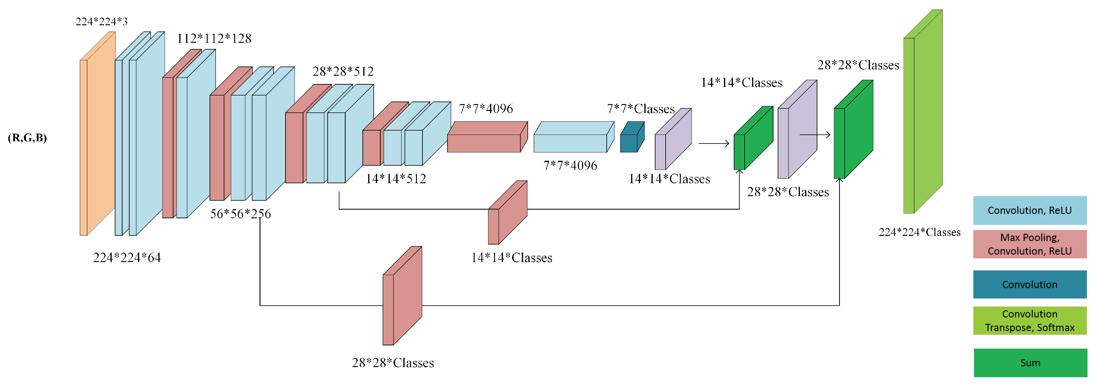
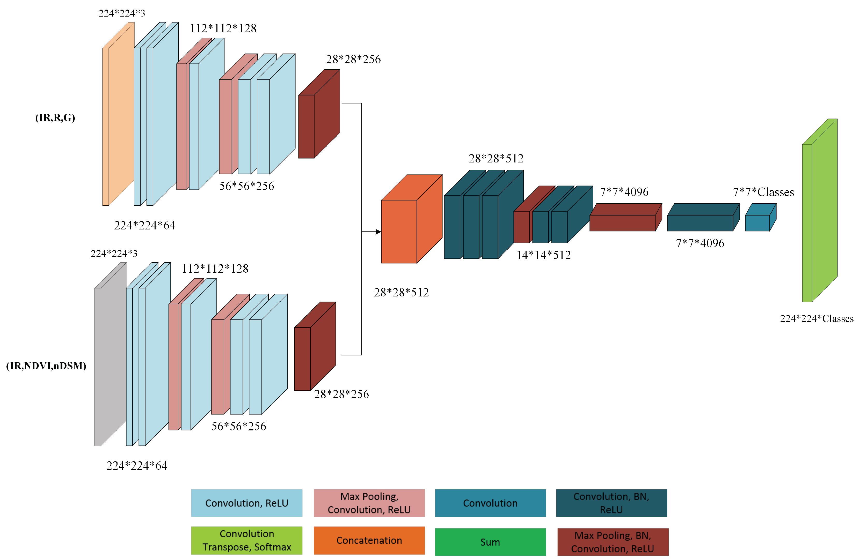
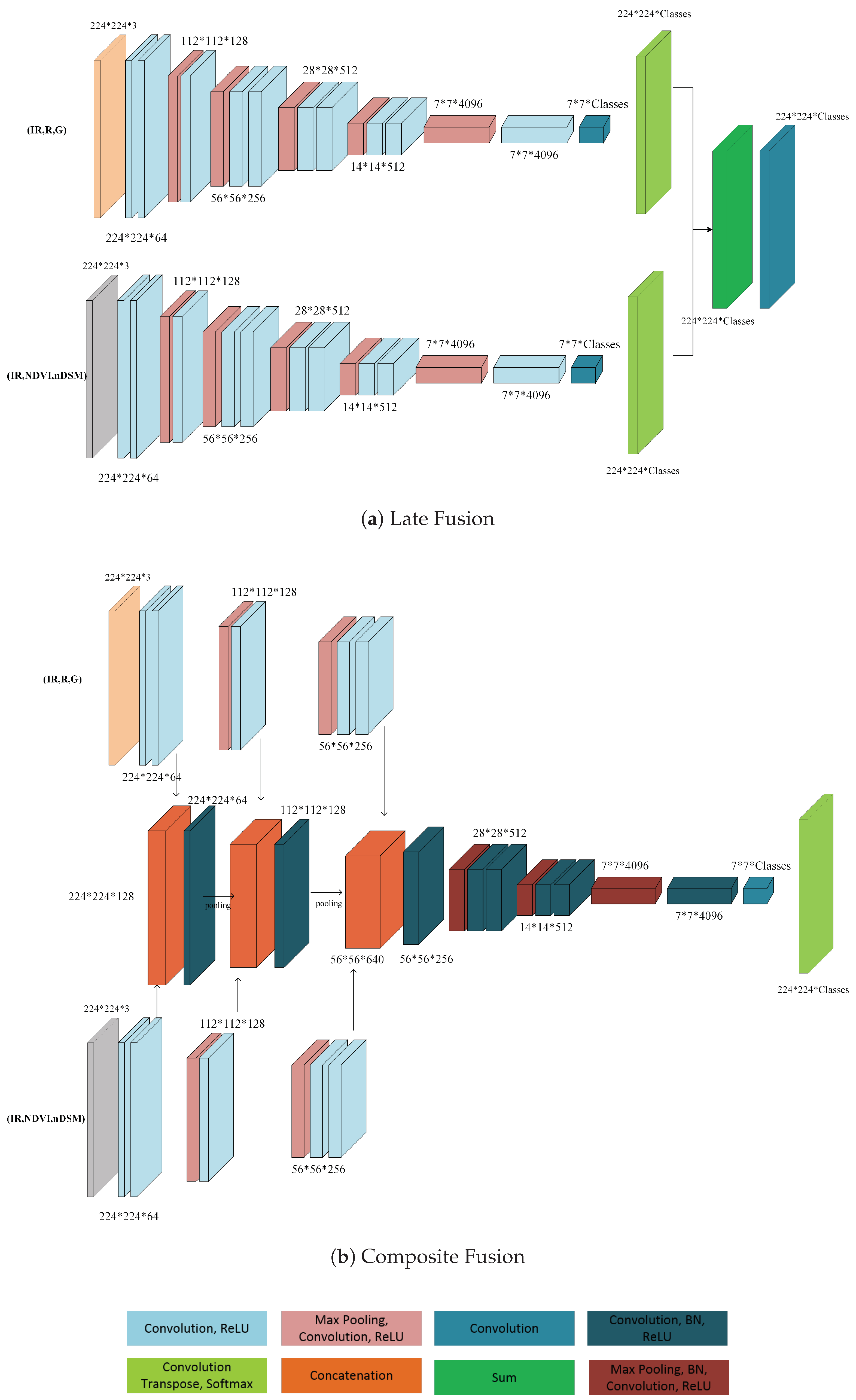
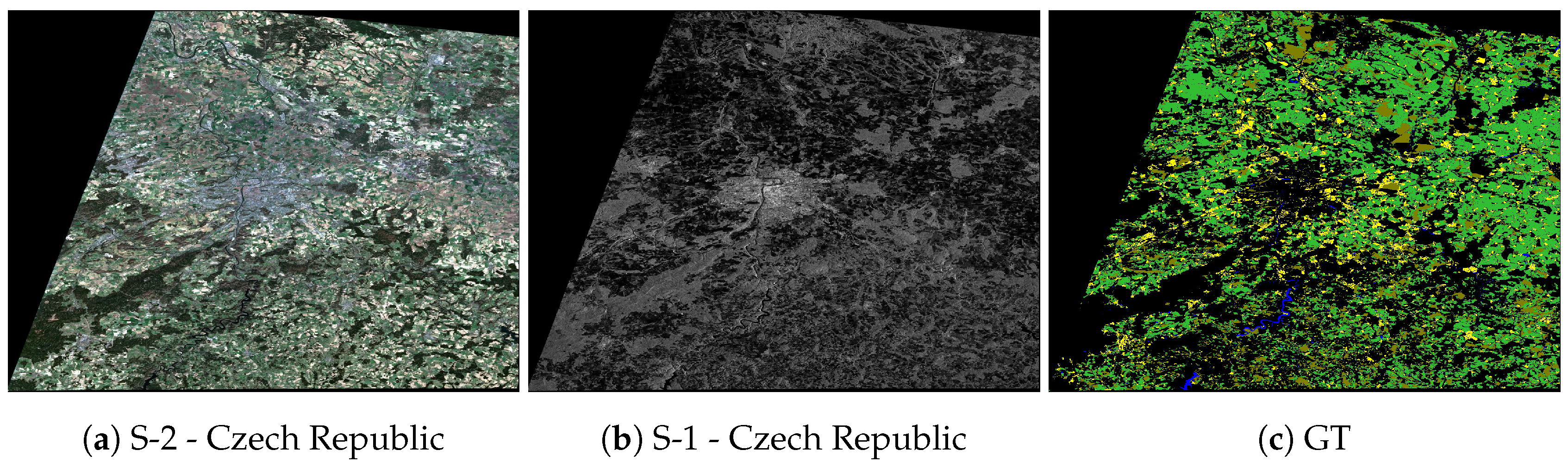
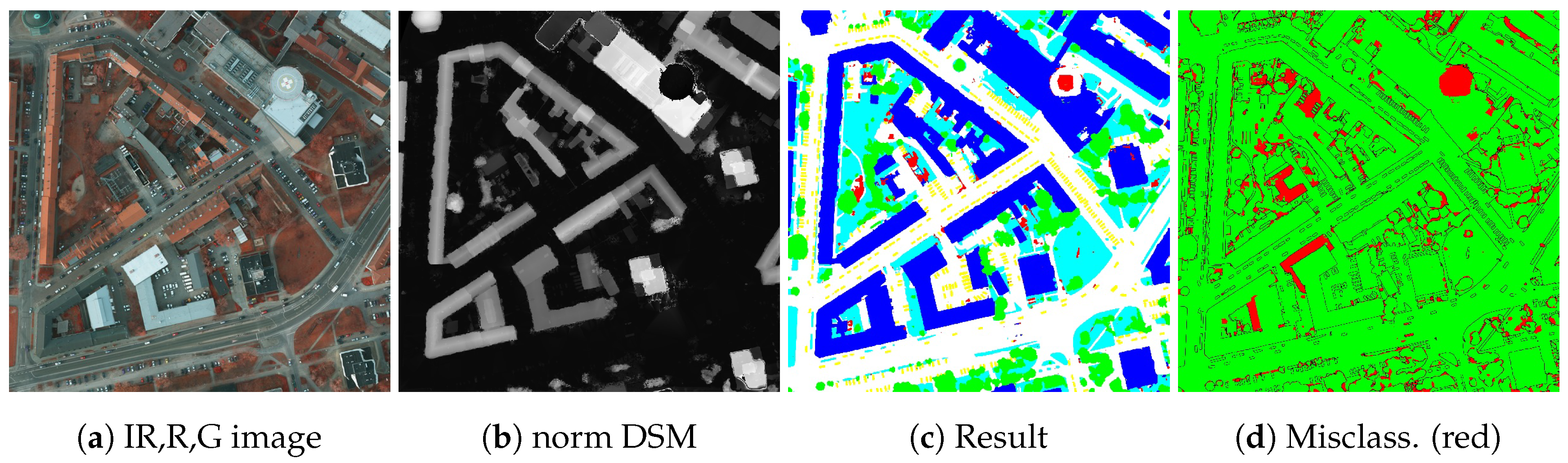
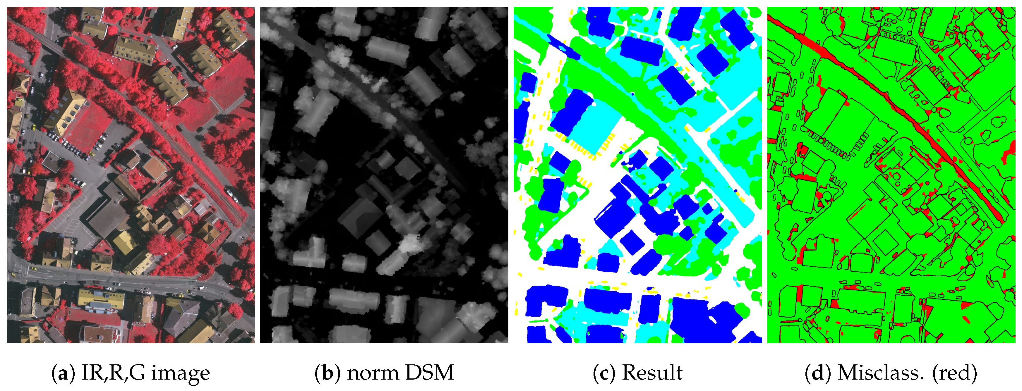
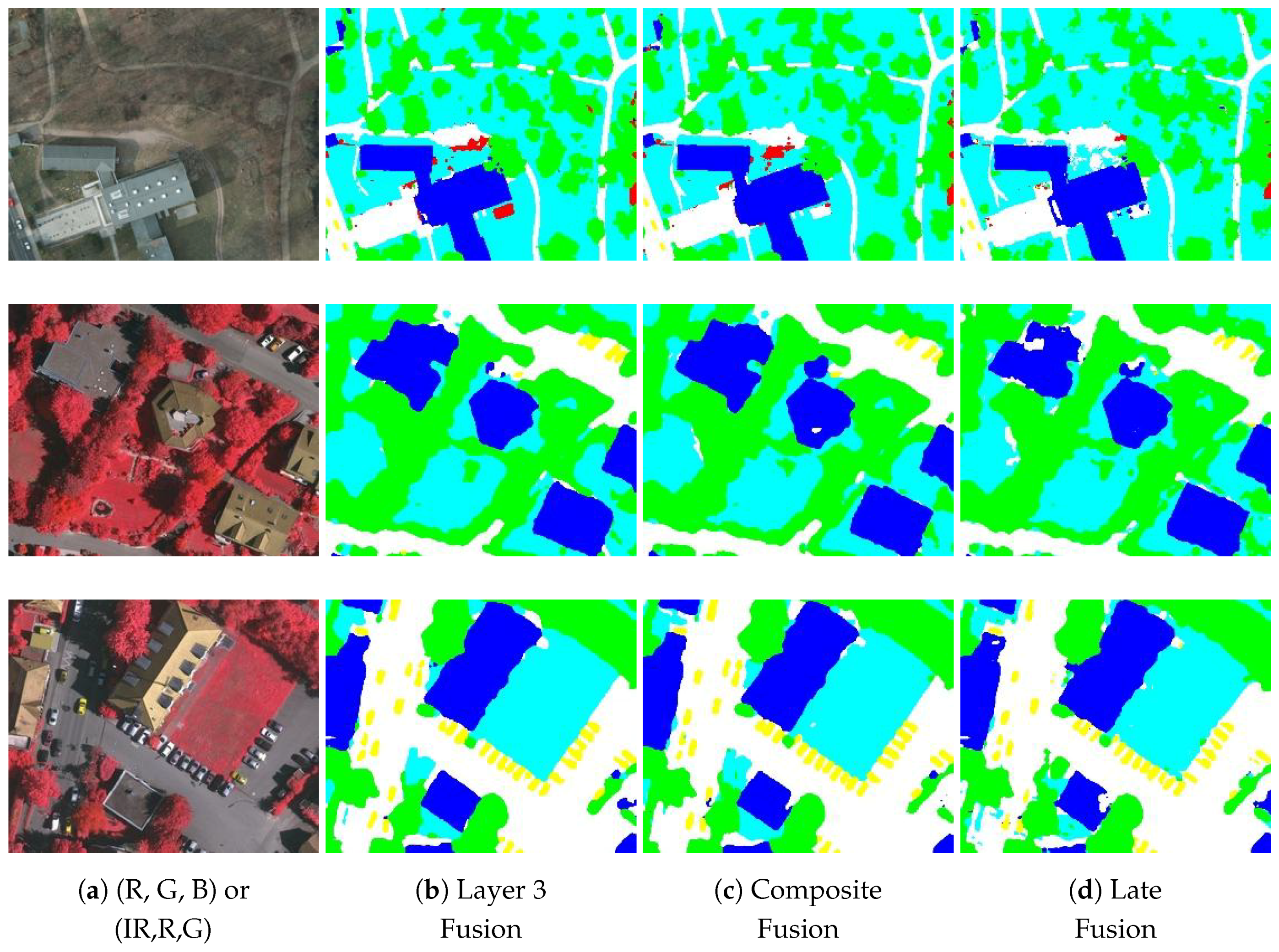
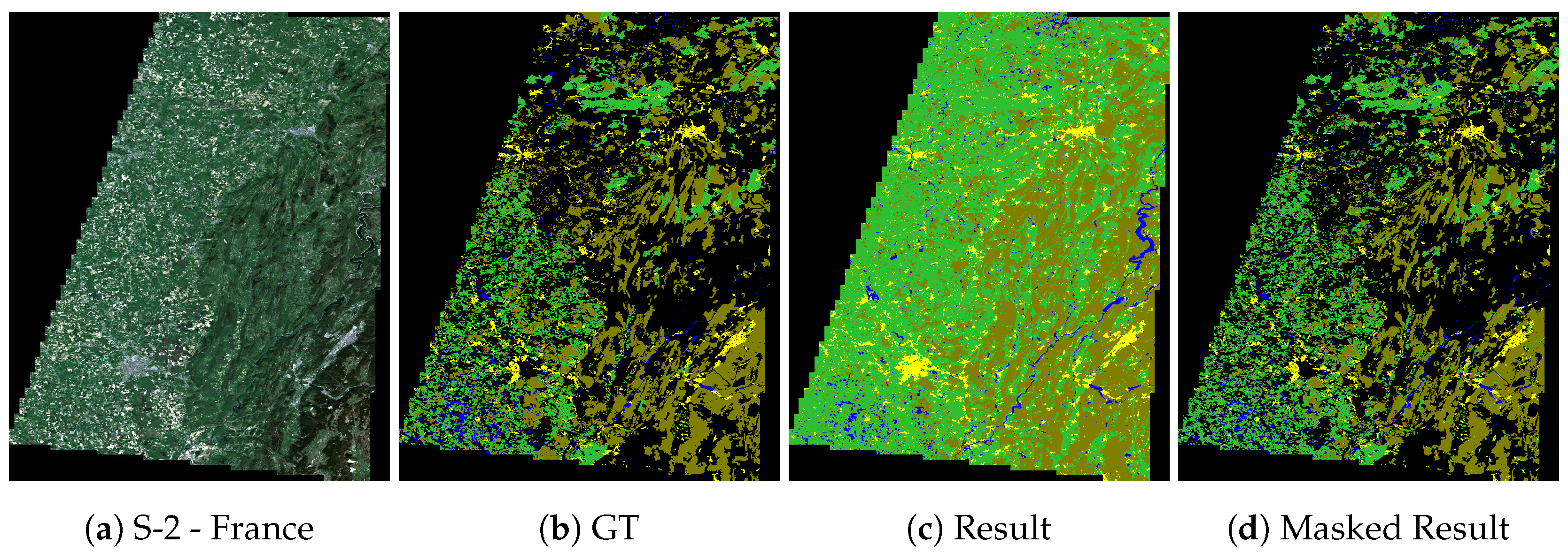
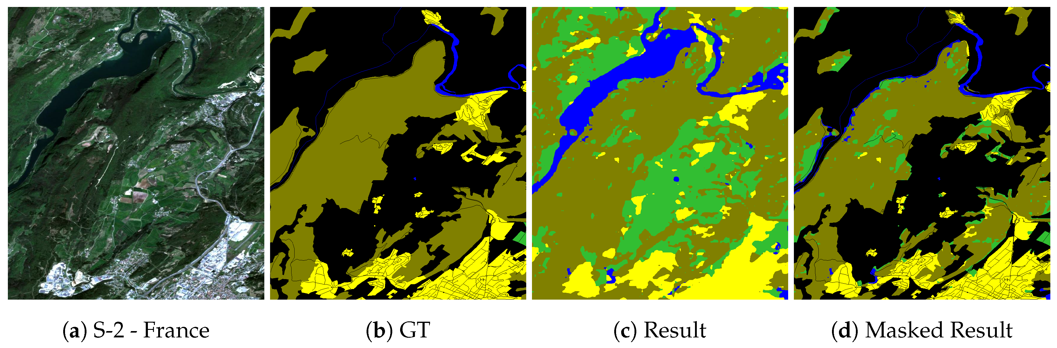
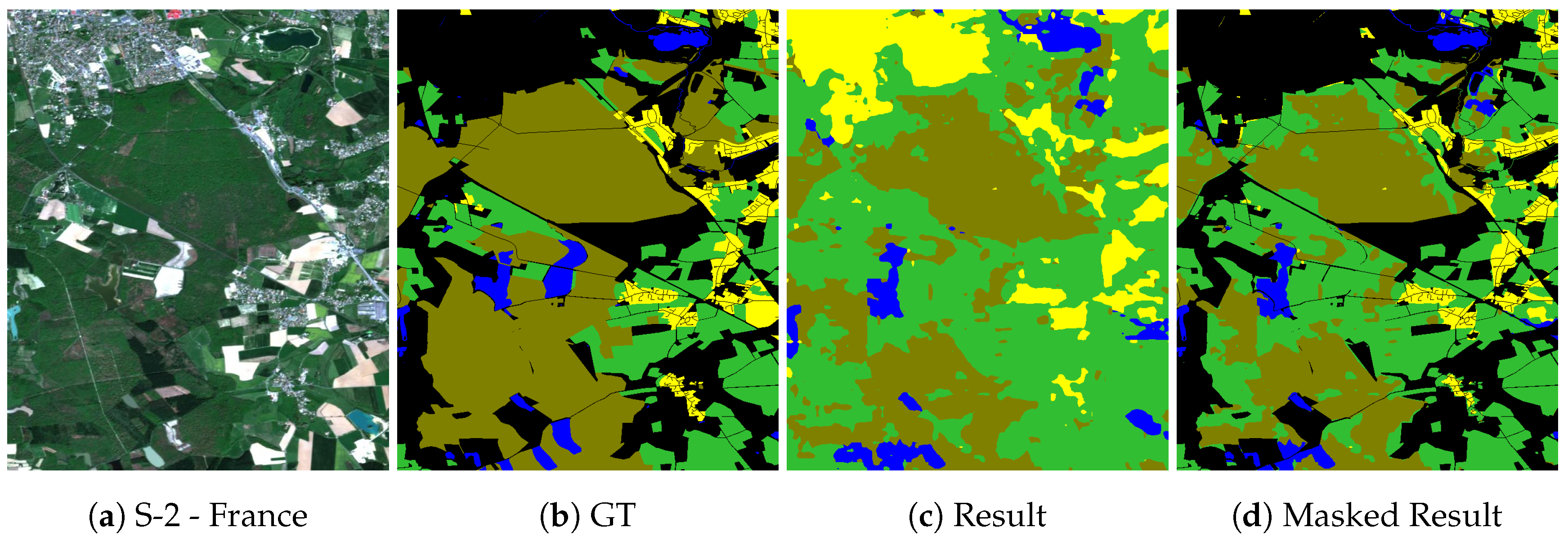
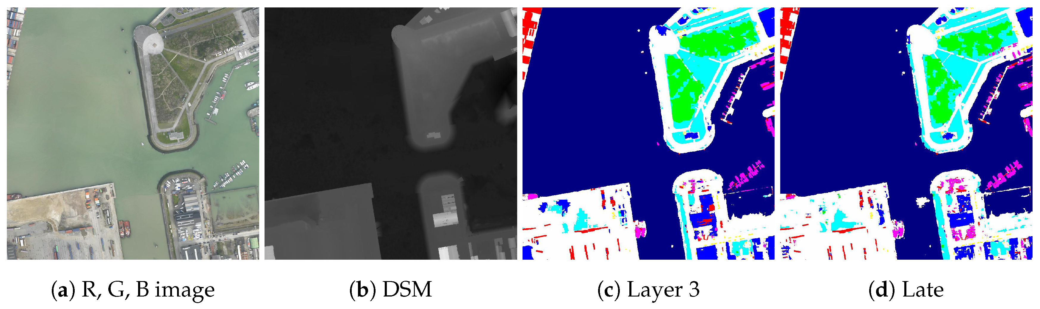
Table 1.
FCN-32 network is trained on image patches obtained from 14 Potsdam training images. The inference is made on remaining 3 Potsdam images and on 3 Vaihingen training images. In the table, LaFsn denotes late fusion, CoFsn denotes proposed composite fusion, LnFsn denotes fusion after layer n. The inputs for the fusion networks were (IR, R, G) & (IR, NDVI, nDSM) channels. The top two results for both image sets are shown in bold-underlined and bold fonts.
| Potsdam Val | Vaihingen Val | |||
|---|---|---|---|---|
| Setup | Overall Accuracy | Average F1-Score | Overall Accuracy | Average F1-Score |
| Pre-trained weights (IR, R, G) | 89.85 | 87.01 | 66.63 | 57.31 |
| Random weights (IR, R, G) | 90.2 | 88.23 | 54.89 | 43.05 |
| CoFsn | 91.51 | 89.5 | 67.95 | 59.39 |
| L1Fsn | 90.43 | 88.28 | 68.86 | 59.02 |
| L2Fsn | 91.23 | 89.20 | 69.11 | 58.57 |
| L3Fsn | 91.36 | 89.27 | 68.89 | 61.91 |
| L4Fsn | 91.03 | 88.88 | 70.65 | 62.91 |
| L5Fsn | 88.42 | 85.52 | 70.39 | 62.09 |
| LaFsn | 90.41 | 87.53 | 72.97 | 63.11 |
Table 2.
Potsdam dataset test results. The fusion networks were tested on (R, G, B) & (IR, NDVI, nDSM) inputs. In the table, LaFsn denotes late fusion, CoFsn denotes proposed composite fusion, L3Fsn denotes fusion after layer 3. Even though, the DLR_10 method produces an overall accuracy 0.6% higher than L3Fsn (shown in bold font), it consists of two neural networks with a comparatively large number of neurons. The NLPR3 achieves the best result (bold and underlined) because of an additional conditional random fields inference step.
| F1-Score | |||||||
|---|---|---|---|---|---|---|---|
| Method | Imp. Surface | Building | Low Veg. | Tree | Car | Avg. 5 Classes | Overall Acc. |
| FCN-8 (R, G, B) [46] | 88.7 | 91.5 | 82.2 | 82.2 | 90.8 | 87.08 | 85.5 |
| L3Fsn (SegNet) | 92.0 | 96.3 | 85.5 | 86.5 | 94.5 | 90.96 | 89.4 |
| L3Fsn (FCN-32) | 92.3 | 96.8 | 86.5 | 87.3 | 91.3 | 90.84 | 90 |
| L3Fsn (FCN-8) | 92.6 | 97.0 | 86.9 | 87.4 | 95.2 | 91.82 | 90.3 |
| LaFsn (FCN-8) | 90.6 | 95.9 | 83.5 | 83.3 | 93.1 | 89.28 | 87.9 |
| CoFsn (FCN-8) | 92.5 | 97.0 | 86.5 | 87.2 | 94.9 | 91.62 | 90.2 |
| DST_5 [45] | 92.5 | 96.4 | 86.7 | 88.0 | 94.7 | 91.66 | 90.3 |
| CASIA2 [11] | 93.3 | 97.0 | 87.7 | 88.4 | 96.2 | 92.52 | 91.1 |
Table 3.
Vaihingen dataset test results. The fusion networks were tested on (IR, R, G) & (IR, NDVI, nDSM) inputs. In the table, LaFsn denotes late fusion, CoFsn denotes proposed composite fusion, L3Fsn denotes fusion after layer 3 (with FCN-8 as a base network).
Table 3.
Vaihingen dataset test results. The fusion networks were tested on (IR, R, G) & (IR, NDVI, nDSM) inputs. In the table, LaFsn denotes late fusion, CoFsn denotes proposed composite fusion, L3Fsn denotes fusion after layer 3 (with FCN-8 as a base network).
| F1-Score | |||||||
|---|---|---|---|---|---|---|---|
| Method | Imp. Surface | Building | Low Veg. | Tree | Car | Avg. F1-Score | Overall Acc. |
| LaFsn | 88.8 | 93.5 | 80.5 | 88.5 | 70.2 | 84.3 | 87.7 |
| L3Fsn | 91.2 | 95.3 | 83.1 | 89.2 | 81.3 | 88.02 | 89.7 |
| CoFsn | 91.7 | 95.2 | 83.5 | 89.2 | 82.8 | 88.48 | 89.9 |
| DST_2 [45] | 90.5 | 93.7 | 83.4 | 89.2 | 72.6 | 85.88 | 89.1 |
| DLR_10 [60] | 92.3 | 95.2 | 84.1 | 90.0 | 79.3 | 88.18 | 90.3 |
| Structured RF [9] | 88.1 | 93.0 | 80.5 | 87.2 | 41.9 | 78.14 | 86.3 |
| NLPR3 [11] | 93.0 | 95.6 | 85.6 | 90.3 | 84.5 | 89.8 | 91.2 |
Table 4.
Quantitative Results for Sentinel-1 and -2 images. LaFsn denotes late fusion, CoFsn denotes proposed composite fusion, L3Fsn denotes fusion after layer 3. The L3Fsn method achieves the best results with a kappa value of 0.6161.
Table 4.
Quantitative Results for Sentinel-1 and -2 images. LaFsn denotes late fusion, CoFsn denotes proposed composite fusion, L3Fsn denotes fusion after layer 3. The L3Fsn method achieves the best results with a kappa value of 0.6161.
| F1-Score | ||||||
|---|---|---|---|---|---|---|
| Method | Water | Farmland | Forest | Urban | Acc. | kappa |
| (R, G, B) | 36.18 | 83.01 | 81.96 | 81.25 | 81.32 | 0.5019 |
| (VH, VV, VV/VH) | 51.53 | 85.02 | 84.80 | 81.87 | 84.87 | 0.5965 |
| (B6, B8a, B11) | 63.71 | 81.24 | 74.57 | 67.48 | 76.07 | 0.3618 |
| L3Fsn (R, G, B) & (B6, B8a, B11) | 55.96 | 87.65 | 85.84 | 82.57 | 85.60 | 0.6161 |
| LaFsn (R, G, B) & (B6, B8a, B11) | 66.82 | 86.38 | 85.07 | 82.54 | 85.11 | 0.6029 |
| CoFsn (R, G, B) & (B6, B8a, B11) | 55.26 | 87.92 | 85.63 | 81.69 | 85.37 | 0.6098 |
| FuseNet [37] (R, G, B) & (B6, B8a, B11) | 54.19 | 87.06 | 85.44 | 84.88 | 85.45 | 0.6120 |
Table 5.
Quantitative results for the Zeebruges test images. In the table, LaFsn denotes late fusion, CoFsn denotes proposed composite fusion, L3Fsn denotes fusion after layer 3. The L3Fsn method achieves the best results with a kappa value of 0.84.
Table 5.
Quantitative results for the Zeebruges test images. In the table, LaFsn denotes late fusion, CoFsn denotes proposed composite fusion, L3Fsn denotes fusion after layer 3. The L3Fsn method achieves the best results with a kappa value of 0.84.
| Method | Imp. Srfc | Bldg | Low Veg. | Tree | Car | Cltr | Boat | Water | Over. Acc. | k |
|---|---|---|---|---|---|---|---|---|---|---|
| L3Fsn | 84.8 | 83.93 | 84.24 | 80.17 | 83.13 | 62.83 | 55.77 | 98.97 | 87.91 | 0.84 |
| LaFsn | 81.67 | 80.20 | 79.99 | 73.64 | 81.86 | 61.47 | 63.71 | 98.59 | 85.22 | 0.81 |
| CoFsn | 81.26 | 76.96 | 74.67 | 77.95 | 82.08 | 57.47 | 50.81 | 98.47 | 83.63 | 0.79 |
| ONERA [55] | 67.66 | 72.7 | 68.38 | 78.77 | 33.92 | 45.6 | 56.1 | 96.5 | 76.56 | 0.7 |
| RGBd AlexNet [13] | 79.10 | 75.60 | 78.00 | 79.50 | 50.80 | 63.40 | 44.80 | 98.20 | 82.32 | 0.78 |
Table 6.
Computational time in ms for the forward and backward pass of the three fusion networks. Time in seconds to generate the result for a test image (France). The test image (France) was divided into 5253 image patches each of size 224 × 224 pixels. In the table, LaFsn denotes late fusion, CoFsn denotes proposed composite fusion, L3Fsn denotes fusion after layer 3.
| Method | Time (ms) | Total Time for | |
|---|---|---|---|
| Forward | Backward | A Test Image (s) | |
| L3Fsn | 19.09 | 49.61 | 163 |
| CoFsn | 23.51 | 57.57 | 185 |
| LaFsn | 28.99 | 86.74 | 212 |
Table 7.
GPU memory consumption at inference time and the number of parameters of the three fusion networks. In the table, LaFsn denotes late fusion, CoFsn denotes proposed composite fusion, L3Fsn denotes fusion after layer 3.
Table 7.
GPU memory consumption at inference time and the number of parameters of the three fusion networks. In the table, LaFsn denotes late fusion, CoFsn denotes proposed composite fusion, L3Fsn denotes fusion after layer 3.
| Method | GPU Inference | Parameters |
|---|---|---|
| Memory (MB) | (M) | |
| L3Fsn | 1826 | 138.44 |
| CoFsn | 2084 | 137.99 |
| LaFsn | 2880 | 268 |
Table 8.
Two-stage results: overall accuracy of Vaihingen and Zeebruges images. The weights obtained after stage 1 and 2 training were used to generate two corresponding test results.
Table 8.
Two-stage results: overall accuracy of Vaihingen and Zeebruges images. The weights obtained after stage 1 and 2 training were used to generate two corresponding test results.
| After 1st Stage | After 2nd Stage | After 1st Stage | After 2nd Stage | |
|---|---|---|---|---|
| Method | Overall Accuracy | |||
| Vaihingen | Zeebruges | |||
| L3Fsn | 89.6 | 89.7 | 87.93 | 87.91 |
| LaFsn | 87.0 | 87.7 | 84.82 | 85.22 |
© 2018 by the authors. Licensee MDPI, Basel, Switzerland. This article is an open access article distributed under the terms and conditions of the Creative Commons Attribution (CC BY) license (http://creativecommons.org/licenses/by/4.0/).
Share and Cite
MDPI and ACS Style
Piramanayagam, S.; Saber, E.; Schwartzkopf, W.; Koehler, F.W. Supervised Classification of Multisensor Remotely Sensed Images Using a Deep Learning Framework. Remote Sens. 2018, 10, 1429. https://doi.org/10.3390/rs10091429
AMA Style
Piramanayagam S, Saber E, Schwartzkopf W, Koehler FW. Supervised Classification of Multisensor Remotely Sensed Images Using a Deep Learning Framework. Remote Sensing. 2018; 10(9):1429. https://doi.org/10.3390/rs10091429
Chicago/Turabian StylePiramanayagam, Sankaranarayanan, Eli Saber, Wade Schwartzkopf, and Frederick W. Koehler. 2018. "Supervised Classification of Multisensor Remotely Sensed Images Using a Deep Learning Framework" Remote Sensing 10, no. 9: 1429. https://doi.org/10.3390/rs10091429
Note that from the first issue of 2016, this journal uses article numbers instead of page numbers. See further details here.