Evaluation of Soil Moisture Variability in Poland from SMOS Satellite Observations


Institute of Agrophysics, Polish Academy of Sciences (IA PAN), Doświadczalna 4, 20-290 Lublin, Poland
*
Author to whom correspondence should be addressed.
Remote Sens. 2019, 11(11), 1280; https://doi.org/10.3390/rs11111280
Submission received: 2 April 2019
/
Revised: 24 May 2019
/
Accepted: 26 May 2019
/
Published: 29 May 2019
(This article belongs to the Special Issue New Outstanding Results over Land from the SMOS Mission)
Abstract
:Soil moisture (SM) data play an important role in agriculture, hydrology, and climate sciences. In this study, we examined the spatial-temporal variability of soil moisture using Soil Moisture Ocean Salinity (SMOS) satellite measurements for Poland from a five-year period (2010–2014). SMOS L2 v. 551 datasets (latitudinal rectangle 1600 × 840 km, centered in Poland) averaged for quarterly (three months corresponding to winter, spring, summer, and autumn) and yearly values were used. The results were analysed with the use of classical statistics and geostatistics (using semivariograms) to acquire information about the nature of anisotropy and the lengths and directions of spatial dependences. The minimum (close to zero) and maximum soil moisture values covered the 0.5 m3 m−3 range. In particular quarters, average soil moisture did not exceed 0.2 m3 m−3 and did not drop below 0.12 m3 m−3; the corresponding values in the study years were 0.171 m3 m−3 and 0.128 m3 m−3. The highest variability of SM occurred generally in winter (coefficient of variation, CV, up to 40%) and the lowest value was recorded in spring (around 23%). The average CV for all years was 32%. The quarterly maximum (max) soil moisture contents were well positively correlated with the average soil moisture contents (R2 = 0.63). Most of the soil moisture distributions (histograms) were close to normal distribution and asymmetric data were transformed with the square root to facilitate geostatistical analysis. Isotropic and anisotropic empirical semivariograms were constructed and the theoretical exponential models were well fitted (R2 > 0.9). In general, the structural dependence of the semivariance was strong and moderate. The nugget (C0) values slightly deceased with increasing soil moisture while the sills (C0 + C) increased. The effective ranges of spatial dependence (A) were between 1° and 4° (110–440 km of linear distance). Generally, the ranges were greater for drier than moist soils. Anisotropy of the SM distribution exhibited different orientation with predominance from north-west to south-east in winter and spring and changed for from north-east to south-west or from north to south in the other seasons. The fractal dimension values showed that the distribution of the soil moisture pattern was less diverse (smoother) in the winter and spring, compared to that in the summer and autumn. The soil moisture maps showed occurrence of wet areas (soil moisture > 0.25 m3 m−3) in the north-eastern, south-eastern and western parts and dry areas (soil moisture < 0.05 m3 m−3) mainly in the central part (oriented towards the south) of Poland. The spatial distribution of SM was attributed to soil texture patterns and associated with water holding capacity and permeability. The results will help undertake appropriate steps to minimize susceptibility to drought and flooding in different regions of Poland.
1. Introduction
Soil moisture (SM) data play an important role in agriculture, hydrology, and climate sciences. In agriculture, soil moisture is a crucial factor for plant growth conditions [1,2], crop water stress [3,4], irrigation scheduling, and soil erosion assessments [5,6]. In hydrology, initial moisture conditions are an important factor in the management of water resources [7] through influence on the splitting (re-distribution) of precipitation into runoff, infiltration, and ground water recharge. These discharges are the most accessible fresh water resources [7]. Almost saturated soil moisture conditions can be a warning of subsequent flooding due to the limited ability of soil to store more water [1,2].
Precise data on soil moisture are a key variable in atmospheric circulation and refining of numerical weather forecasts, whereas improper initial SM results in incorrect climate predictions [8,9]. Knowledge of the exchange of water and energy between the soil and the atmosphere contributes to improving crop growth conditions and hydrological models [7,10] and potential landslide predictions [11]. Moreover, many researchers indicate that SM indirectly influences other significant soil properties, including aeration, mechanical impedance, and temperature that affect numerous soil and plant functions [12,13].
Several evaluations and comparisons of remote SM have been made using observations from in situ measurements [14]. They are fairly accurate for point-based measurements, however inadequate to perform SM evaluation on larger scales [15]. This problem is gradually solved with the development of remote sensing techniques. The most suitable for the retrieval of soil moisture are microwave (satellite) observations from active and passive sensors [16,17,18]. The SMOS (Soil Moisture and Ocean Salinity) satellite mission of the European Space Agency [19] provides soil moisture observations by means of the interferometric radiometry method (1.4 GHz) from the orbit, ranging from regional to global scales and at a temporal resolution of three days. The satellite measurements of SM made by SMOS began on November 2009 [20] and are spatially continuous and fast, thus coherent. It is the first mission particularly designed to obtain SM from space [19].
The main limitation of the remotely SM sensed data is their range of top few centimetres of soil [7,21]. To overcome this limitation, the surface SM products provided by remote sensing are gradually refined to increase their usefulness and applicability. An example can be assessment (integration) of plant available water at 0–50 cm depth from the SMOS surface soil moisture using the Soil Water Index (SWI) as a proxy of the root-zone soil moisture [22]. Moreover, SWI was found to be a suitable and cheap supplementary tool for drought monitoring using the SMOS soil moisture data [23]. In Poland, droughts are determined by means of a Climatic Water Balance (CWB) based on the differences between atmospheric precipitation and potential evapotranspiration (approximating the ability to evaporate water from a well-watered grass) calculated using the Penman method [24]. SMOS data supplements the CWB’s information on soil moisture, which allows the indication of soil moisture conditions suitable for plant growth, and threats of droughts and floods. Comparisons of SMOS data against in-situ SM measurements showed good values of correlation (R > 0.7) [25,26] and relatively low RMSE (i.e., 0.04 m3 m−3) [7,22,26].
The aforementioned studies imply that the SMOS data can be useful for important applications in agriculture and hydrology, although further research on the evaluation of spatial distribution and refining soil moisture data and algorithms, especially for larger scales and longer periods, is required [7,27]. Therefore, in this study, we examined the spatial-temporal variability of soil moisture using SMOS satellite observations in Poland for 2010–2014.
2. Materials and Methods
In this study, the SMOS L2 v. 551 datasets for Central and Eastern Europe (latitudinal rectangle 1600 × 840 km, centered at Poland) were examined. The statistical features of soil moisture distributions of this area were studied for quarterly (three months) averaged SMOS data for 2010–2014. The I, II, III, and IV quarters during the year correspond to winter, spring, summer, and autumn, respectively. The total number of data was about 5000. After pixel regularization, geostatistical methods were applied directly on the Discrete Global Grid (15–km grid) using the Icosahedral Snyder Equal Area (ISEA) map 4H9 projection, on which SMOS data is provided.
Descriptive statistics and characterization of spatial variation were performed by GS+ Version 9 (Gamma Design Software, 2008, Plainwell, MI, USA) including the mean, standard deviation (STDev), maximum, minimum, skewness, kurtosis, and coefficient of variation (CV) [28]. Histograms for the soil moisture content data were inspected for characterization of spatial variation. The datasets were also checked for required normality and root square transformed where needed before calculation of the experimental semivariograms [29]. The semivariograms were calculated from the equation:
where γ(h) is the semivariance for interval distance class h; z(xi) is the measured sample value at point xi; z(xi+h) is the measured sample value at point xi+h; and N(h) is the number of distinct data pairs for the lag interval h. The theoretical exponential models were fitted to the experimental semivariograms γ(h) using the weighted nonlinear least square method to minimize the residual sum of squared errors (RSS) between experimental semivariance data and the models by optimizing the model parameters: nugget, sill, and range values.
We used the exponential isotropic and anisotropic models:
where, γ(h) is the semivariance for internal distance class h, h is the lag interval, C0 is the nugget variance ≥ 0, C is the structural variance ≥ C0, A = A0 is the range parameter (isotropic). In the case of the exponential isotropic model, the range (or effective range) for the major axis is 3 A0, which is the distance at which the sill (C0 + C) is within 5% of the asymptote (the sill never meets the asymptote in the exponential model):
(anisotropic), A1 is the range parameter for the major axis (φ). In the case of the exponential anisotropic model, the range (or effective range) for the major axis is 3A1, and A2 is the range parameter for the minor axis (φ + 90). The range in this model for the minor axis is 3A2, φ is the angle of maximum variation, and θ is the angle between pairs. The ratios C0/(C0+C) <0.25, 0.25–0.75, and >0.75 indicate strong, moderate, and weak spatial dependence, respectively [30]. The minimal anisotropy for the chosen azimuth transect was calculated with consideration of the major (lower average semivariance) and minor (90°-offset) directions using the anisotropic semivariogram model.
To characterize the nature of spatial soil moisture variability, we calculated the fractal dimension (D(0)) using the slope (m) of the log–log semivariograms plots from the formula [28,31]:
As we did not assume isotropy for our data, the fractal dimension describes surface variability of soil moisture and varies from 1 to 2.
3. Results
3.1. Descriptive Statistics of Soil Moisture
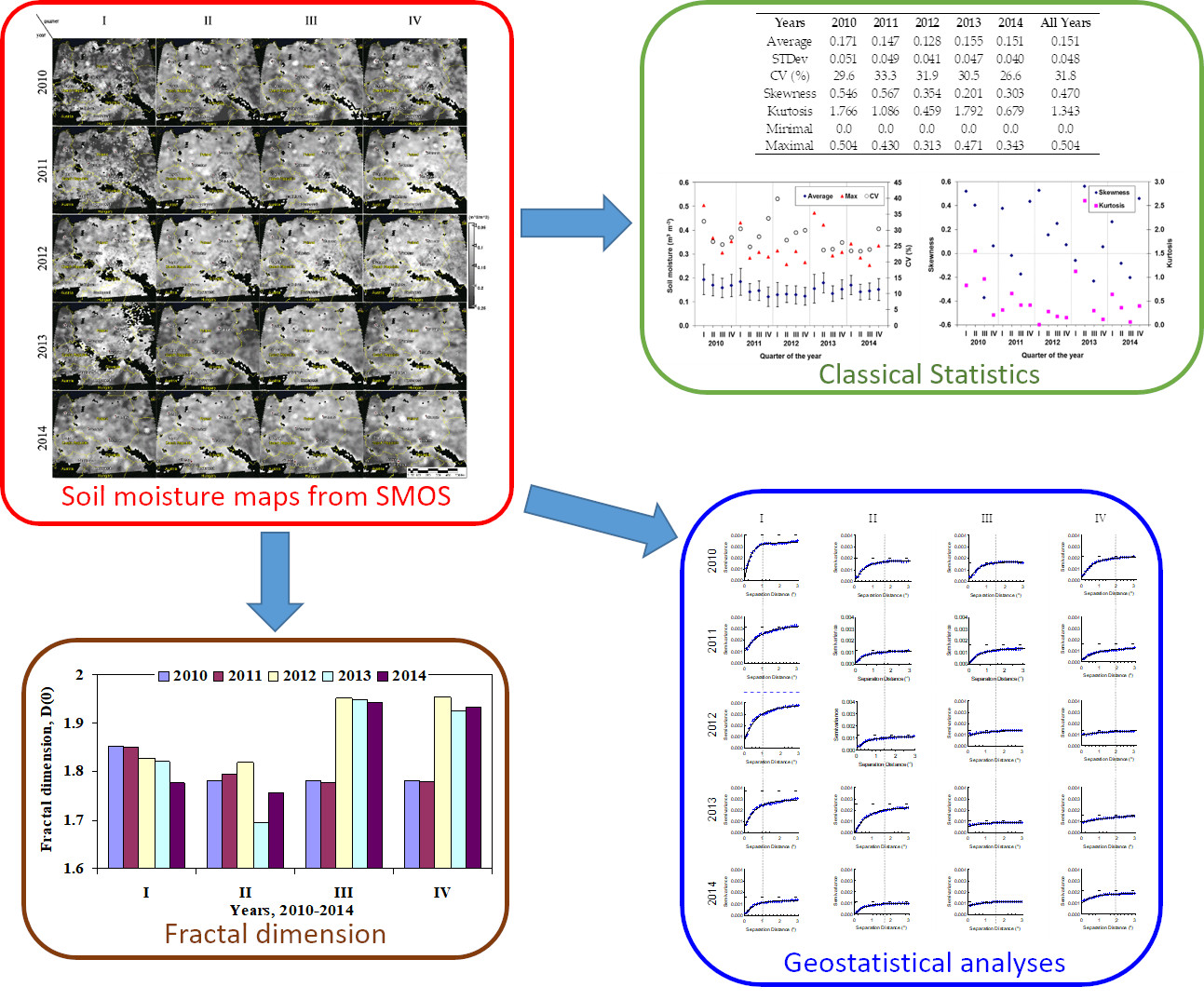
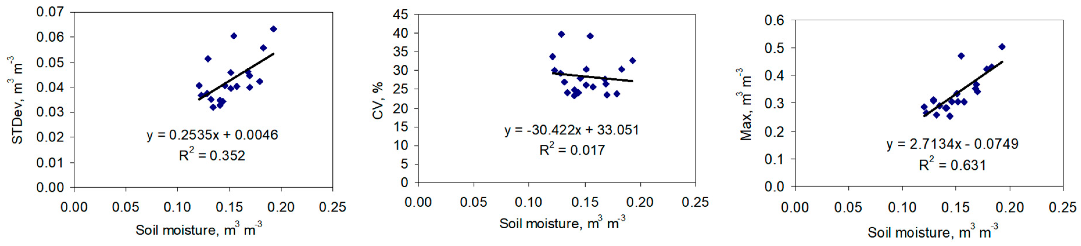
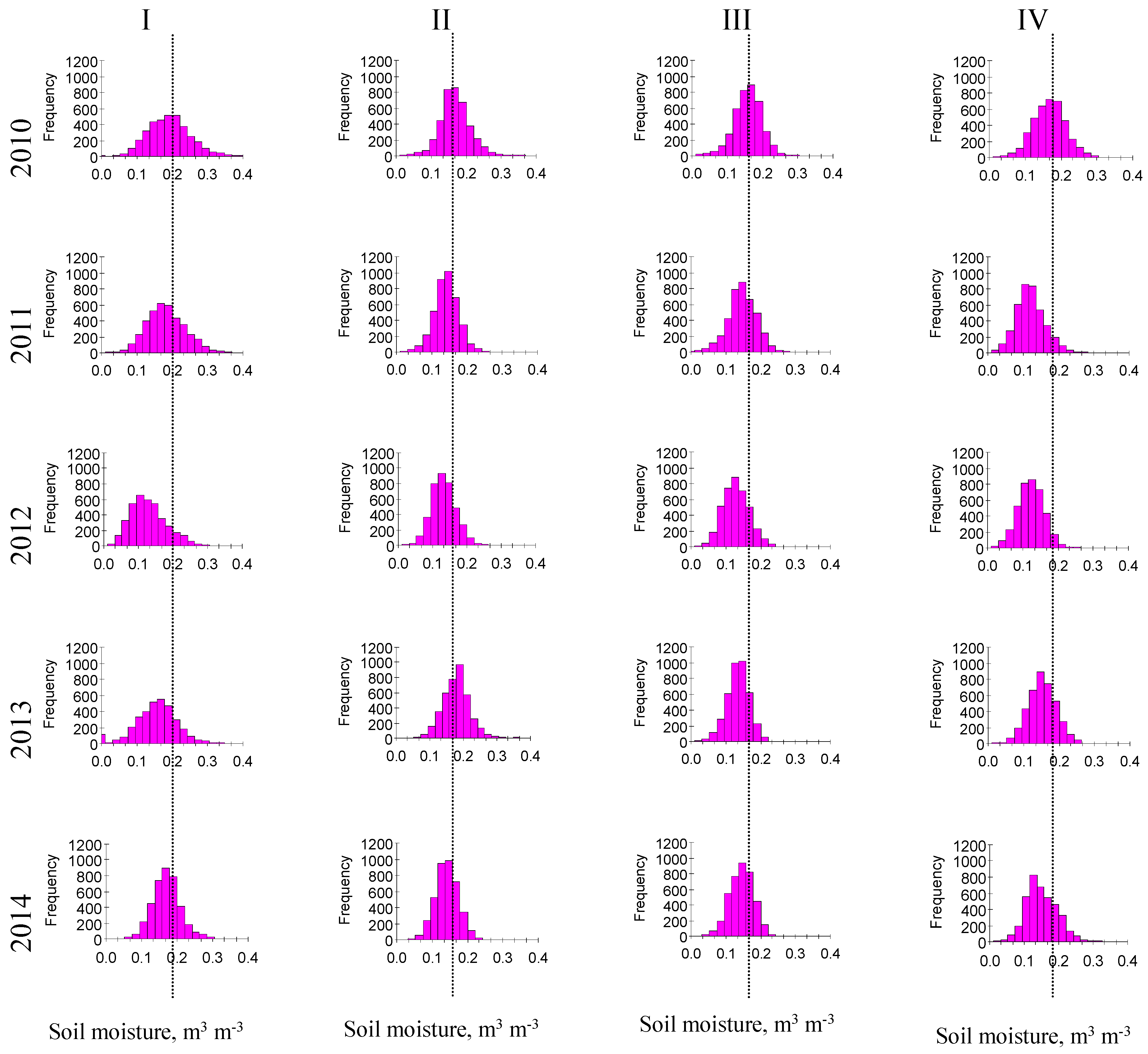
Table 1 presents annual statistics for 2010–2014 individually and all years combined. The soil moisture averaged for the entire five-year period was 0.151 m3 m−3, with the highest value in 2010 (0.171 m3 m−3), which dropped to 0.128 m3 m−3 in 2012. Year 2010 was the rainiest in Poland in the postwar period [32]. The significant snowfall in 2013 caused an increase in soil moisture by 0.027 m3 m−3. In the subsequent year, the average soil moisture decreased again, but much less than before (in the 2010–2012 period). The CV was similar in all years (26.6–33.3%). The distribution of SM was positive and slightly narrow, as indicated by skewness (0.20–0.57) and kurtosis (0.46–1.79). The minimum (close to zero) and maximum soil moisture values covered the 0.5 m3 m−3 range. Basic quarterly statistics for each year are given in Figure 1. In the particular quarters, the average soil moisture did not exceed the 0.2 m3 m−3 value and did not drop below 0.12 m3 m−3. In general, the lowest values appeared in summer (quarter III) and the highest in winter (quarter I) (Figure 1). As indicated by CV, the highest variability of SM occurred generally in winter (up to 40%) and the lowest value of approx. 23% was noted in spring. The yearly dispersions (standard deviations) varied from 0.04 m3 m−3 to 0.051 m3 m−3. The value was approx. 6.3% in winter and lower (up to ca. two-fold) in the other quarters. Variability expressed by the coefficient of variation was over 33% in each particular year and nearly 40% in the first quarter of 2012 and 2013, with balanced (equalized) and lower variability in the spring and summer and increased again in the autumn. The skewness was in general positive in winter, negative in summer, and positive or close to zero in spring and autumn. The skewness and kurtosis values indicate that the SM distribution was predominantly close to normal. Figure 2 indicates trends between the standard deviation (STDev), CV, maximum soil moisture content (Max), and average soil moisture. The trends were increasing for STDev and Max and slightly decreasing for CV. The trends are moderately strong in case of STDev and Max and weak in case of CV. Histograms of soil moisture distribution with lines of quarterly averaged soil moisture values for 2010–2014 using 2010 as a reference are presented in Figure 3. The concentration of the distribution around the average was greater in spring and summer than in autumn and winter. The asymmetries were negative only in the summers, but mostly positive in the other seasons. To perform further analysis of data using geostatistical methods, the distributions with the highest asymmetry were transformed with square root to obtain normal distribution. The negative asymmetry in the summer periods (with the predominance of lower soil moisture values) indicated an increase in dry areas. This is related to the fact that soils rich in sand fraction dominate in the central part of Poland. Lack of precipitation, already developed vegetation, and higher temperatures may have even further reduced the moisture in the surface layer of soil. Negative skewness was sometimes noted in the spring, when the rainfall amount was low and the temperatures were high.
3.2. Semivariograms
Most of the measured soil moisture distributions were close to normal distribution (Figure 3) and thus met the primary condition of geostatistics, which facilitated further analysis of spatial variability using semivariograms and fractal dimension.
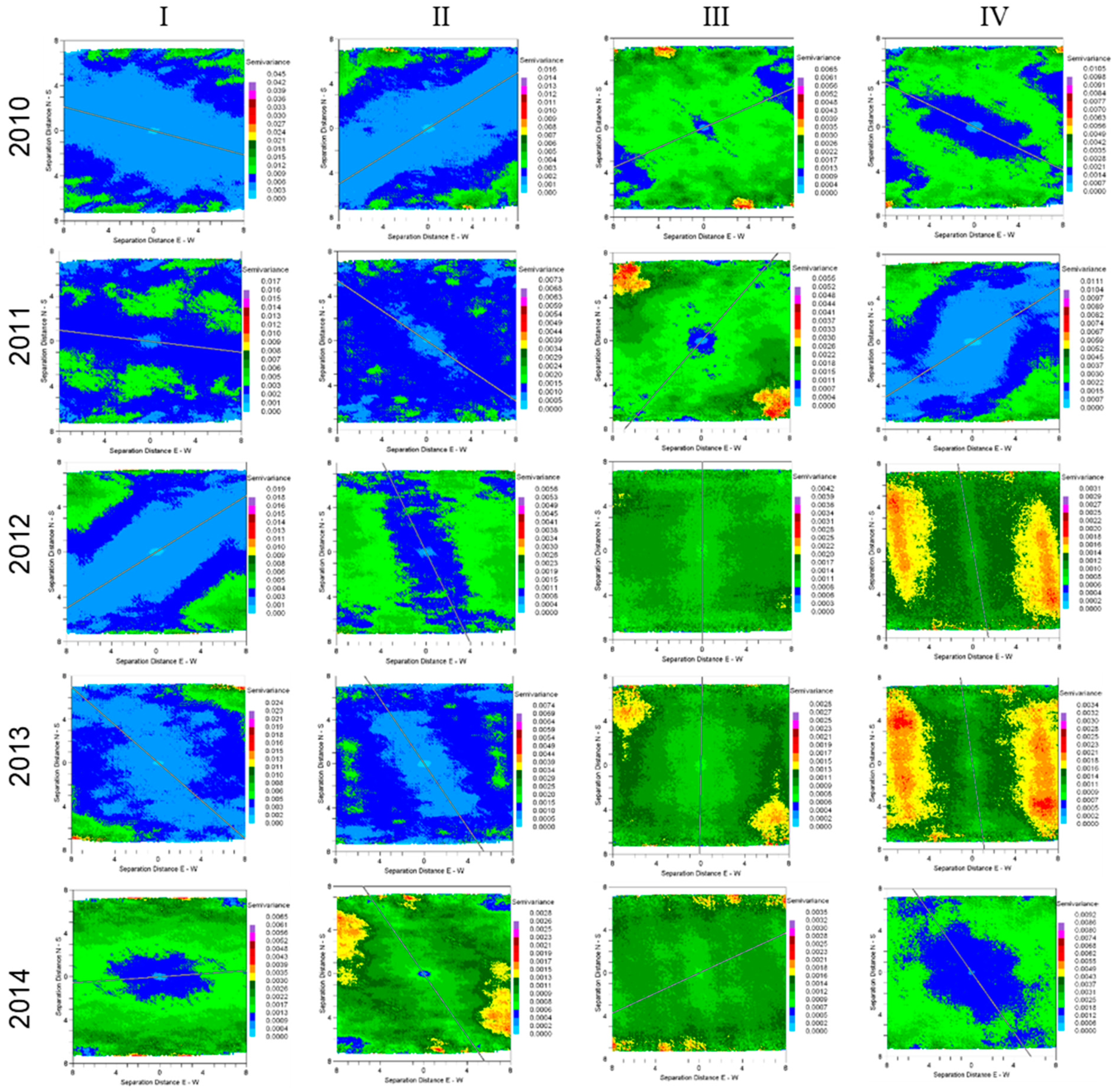
The isotropic semivariograms, anisotropic semivariograms, and geostatistical parameters of soil moisture for quarters I, II, III, and IV in 2010–2014 are presented in Figure 4 and Figure 5, and Table 2, respectively. For every quarter, empirical semivariances were determined and the theoretical models adjusted to them. The fitting was in good agreement with the coefficients of determinations (R2 > 0.9) and small residual sums of square errors (RSS < 1.5 × 10⁻⁷). In all the examined quarters, the nature of the spatial changes in the studied distributions of soil moisture was described by an exponential model of semivariance. The structural dependence of the semivariance was in general strong in all quarters during the first two study years (C0/(C0 + C) < 0.25). It was strong in the winter-spring period (I and II quarters) and moderate during the summer and autumn (III and IV quarters) in the last three examined years (C0/(C0 + C) < 0.75) according to [30]. The nugget (C0) values slightly declined with the increasing soil moisture, while the sills (C0 + C) increased. The sill values were generally the highest in the winter periods and significantly reduced (up to more than three times) in the other quarters (Figure 3, Table 2). The greatest variations of soil moisture were observed during winters (Figure 1a and Figure 3). The effective ranges of spatial dependence (A) were between 1° and 4°, which corresponds to approximately 110–440 km of linear distance (Table 2). Comparison of the results indicates that, generally, smaller ranges were noted for moist soils (e.g., range 0.999° in Table 2 and Figure 4 for the moist quarter I in 2010 in Figure 1; Figure 3) and increased for drier soils (e.g., range 4.083 in Table 2 and Figure 4 for the dry quarter IV in 2013 in Figure 1 and Figure 3).
The parameters of anisotropy for semivariance and related maps of anisotropic semivariograms with the lines of minimal anisotropies are shown in Table 2 and Figure 5, respectively. They show different orientation of the minimum values of surface semivariation of soil moisture in the individual quarters and years (Figure 5). At relatively high soil moisture contents, which occur mainly in winter and spring (Figure 1; Figure 3), the direction of semivariation from north-west to south-east is dominant. As soil moisture decreases in the other quarters, the orientation changes from north-east to south-west or from the north to the south (Figure 5). Such distribution of the minimum semivariations for soil moisture is determined mainly by the nature and size of precipitation. In the winter, early spring, and late autumn, at relatively high soil moisture contents, the frontal precipitation from the north-west direction prevails, whereas point precipitations dominate in summer [33] and then the soil moisture distribution is largely influenced by soil texture [34,35]. These orientations of minimum semivariations of soil moisture were reflected in the orientation of the minimum semivariance of sand and silt from west to east and clay, which does not show a clear direction and is close to isotropic distribution.
3.3. Fractal Dimension
Fractal dimension was determined with a good agreement (coefficients of determinations >0.85, standard error <0.15). As can be seen from Figure 6, the obtained values of fractal dimensions ranged from about 1.7 to over 1.95. Lower values of the fractal dimension were observed during the winter and spring, indicating smoother (less diverse) distribution of repeated patterns of soil moisture at the time (Figure 7). From winter to autumn, the fractal dimensions did not change substantially in the first two examined years (2010–2011). In the following years, a decrease in the fractal dimension in the winter-spring period and a significant increase in the summer-autumn period were observed. The increase in the fractal dimension indicated that the number of areas differing in soil moisture content increased (Figure 7) with the increasing share of sites with lower soil moisture (white spots). The least diversified soil moisture was noted in spring 2013 (fractal dimension approximately 1.70) and the highest diversity was reported in autumn 2012 (fractal dimension approx. 1.95).
3.4. Soil Moisture Maps
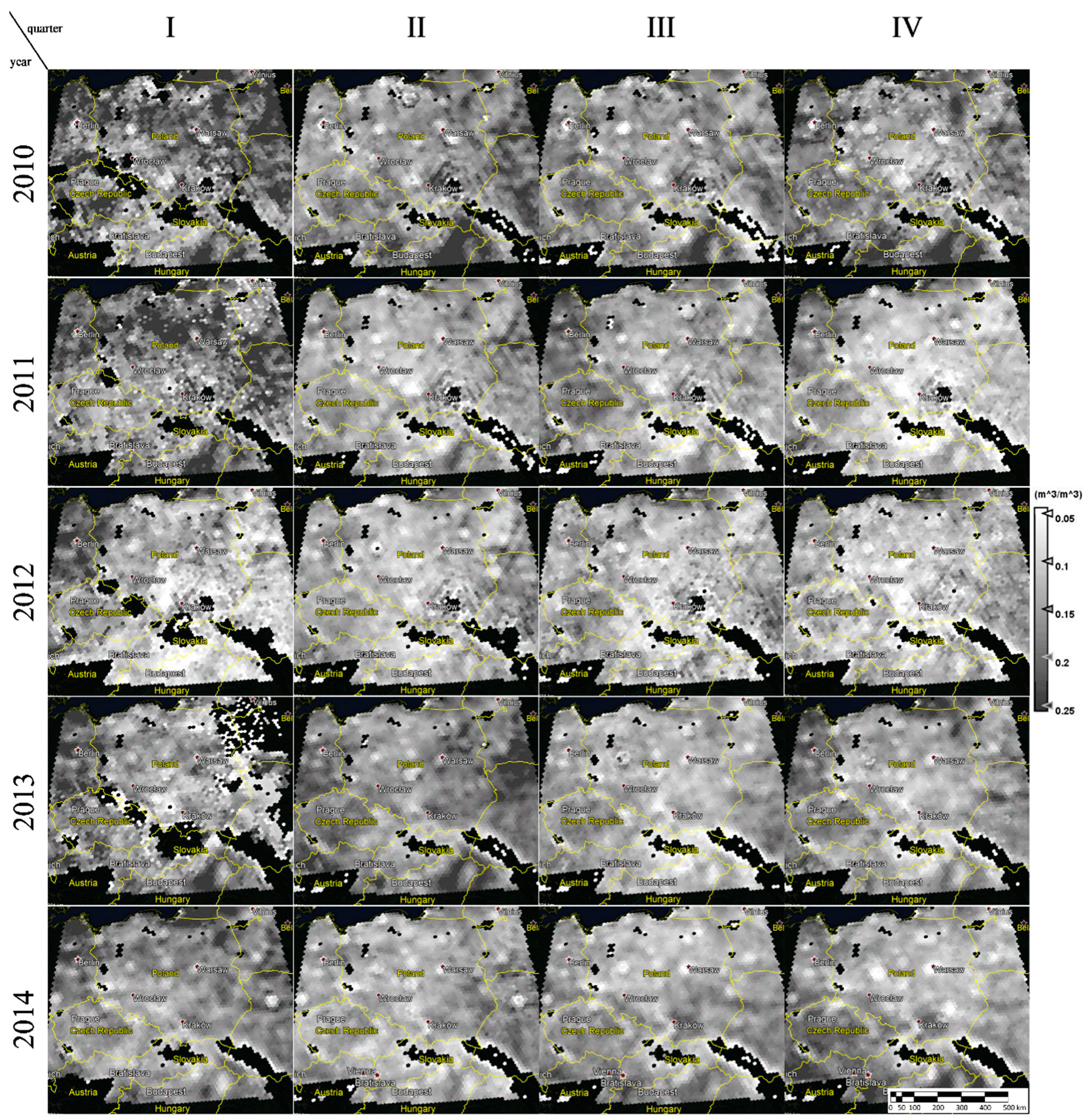
The maps of soil moisture in Poland and parts or whole areas of neighbouring countries in quarters in 2010–2014 are presented in Figure 7. The maps show that the averaged values of soil moisture in general ranged from 0.05 m3 m−3 to 0.25 m3 m−3, including single data below or above this range (Figure 3). Values below 0.05 are marked in light colour and those above 0.25 m3 m−3 are dark (Figure 7). It is worth noting that the areas in the north-eastern, south-eastern, and western parts of Poland are relatively wet throughout the periods in all the study years. However, less wet areas (lightened) occur mainly in central Poland and are oriented towards the South. The maps indicate that the entire year 2010 was moist across Poland, whereas in 2011 only the northern part of Poland was moist in winter (1st quarter), in contrast to the much less moist southern Poland. A decrease in soil moisture was then observed, which persisted until the winter of 2013, followed by an increase in spring and again a slow decrease until the end of 2014 (Figure 1, Figure 3, Figure 5 and Figure 7). Recognizing and understanding the causes of the low soil moisture in these regions would enable appropriate steps to be taken to minimize drought.
To show the reliability of maps in Figure 7, time series of precipitation obtained from the Polish meteorological stations [32] were compared with soil moisture from chosen SMOS pixels in different parts of Poland (Figure 8). Those time series show moderately good compatibility of trends; in particular, one may observe increase in soil moisture after rainfall. However, this phenomenon is not always proportional to the amount of precipitation due to surface runoff, drainage, intensive evaporation, presence of vegetation, different soil textures, etc.
4. Discussion
The results show that the temporal variations and spatial distribution of soil moisture were related to precipitation [32], soil texture (i.e., fraction of sand, silt, and clay), and hydrophysical characteristics, including water holding capacity presented in the databases for Polish arable mineral soils [36,37]. The largest average SM observed in most years in the first quarter (winter) (except 2012 and 2013) was mainly related to the recharge of precipitation as well as low temperature and evapotranspiration [38]. This recharge was further reflected in higher soil moisture in spring than in summer, except 2013 due to the long persistence of snow until the end of April. The spatial distribution of soil moisture along with the orientation of the minimum semivariance values was largely related to the soil texture pattern, as indicated by the orientation of the minimum semivariance of sand and silt from West to East and clay that did not show a clear direction and was close to isotropic distribution [35]. The lowest soil moistures (<0.05 m3 m−3) observed in Central Poland can be related to the presence of permeable soils with relatively coarse texture [34], poor water holding capacity, and deep ground water level [36,37]. Therefore, the soils can barely be supplied with water following rainy seasons. Furthermore, the SM data indicate that the soils in Central Poland are susceptible to an agricultural drought risk [23]. Susceptibility to drought of this part of Poland was also indicated by other drought indices based on national Climatic Water Balance (CWB) determined from precipitation and potential evapotranspiration data [24]. The low soil moisture and spatial-temporal variability in this region can further be enhanced by intensive agricultural activity with diverse crop rotation, generally without irrigation (rain-fed agriculture). However, the higher soil moisture in some other regions e.g., the north-western, north-eastern and south-eastern parts of Poland, can be a result of predominance of relatively finely textured mineral soils and/or peat soils with high water holding capacity [36,37]. The results imply that different soil (agricultural) management practices should be applied to improve soil water relations depending on the local SM conditions. In relatively dry areas covered by coarse-textured soils, the use of water-saving or lower water-requirement crop types or varieties [39,40,41] along with low planting density can alleviate water shortage. In a longer time span, application of exogenous organic materials including biochar or conservation tillage systems with the use of intercrops can be a relevant solution [42].
It is worth noting that the relations between SM from SMOS and soil texture are of particular value, as the latter does not vary over time. The suitability of soil texture can be enhanced since SMOS is particularly efficient at monitoring SM over sparse vegetation [7].
The evaluation of the SMOS SM long-term (2010–2014) datasets in the country scale made in this study can be a useful contribution to various applications, including examination of climate change trends, flood analysis, and/or drought monitoring at smaller scales including e.g., the commune. The value and applicability of SMOS surface soil moisture data at the coarse spatial resolution can be enhanced by new developments. Some approaches allow disaggregation of soil moisture (from large pixels) to provide soil moisture data in the scales from several kilometres to several meters. They are based on the synergy of passive microwaves with ancillary optical visible/infrared (VIS/IR) [43,44] or active data [45]. Another approach allows assessment of plant available water at the 0–50 cm depth from the SMOS surface soil moisture based on the Soil Water Index (SWI) as a proxy of the root-zone soil moisture [22]. The SWI is also used as a proxy of drought [23].
The usefulness of the SMOS data can be further enhanced by the significant linear relationship between the current SM and maximum soil moisture derived from SMOS data (Figure 2, R2 = 0.63) in the present study. The increased maximum soil moisture content with the increasing current SMOS SM content can be largely associated with the greater clay content and soil aggregation containing big structural inter-aggregate pores in soil matrix [46]. These pores accelerate the flux of water, i.e., preferential flow, under ponded (saturated) conditions [12]. Preferential flow is a key component of water movement in many soils, especially in fine textured soils. It allows alleviating the risk of soil surface runoff and erosion on the one hand [11] and permits solutes to bypass parts of the soil, thereby leading to faster transport from soil surface to groundwater on the other hand [47,48]. Moreover, a large contribution of these pores in saturated soil can raise the quantity of water that is not available for plants due to insufficient aeration. However, under non-ponded conditions, the big pores (macropores) filled with air will increase gas diffusion and improve soil aeration [49].
5. Summary and Conclusions
Spatial distributions and variability of soil moisture obtained from SMOS data for Poland was analysed and evaluated for the years 2010–2014. The soil moisture values in the seasons (quarters) varied from close to zero to 0.5 m3 m−3 and average values from 0.128 to 0.171 m3 m−3. The highest variability of soil moisture generally occurred in winter (coefficient of variation, CV, up to 40%) and the lowest values were noted in spring (CV around 23%). A positive correlation between the quarterly maximum (Max) soil moisture contents and the average soil moisture contents (R2 = 0.63) was established.
The isotropic and anisotropic empirical semivariograms showed that the structural dependence of the semivariance was strong and moderate. The ranges of the spatial dependencies from 1° and 4° (110–440 km of linear distance) were in general greater for dry than moist soils. The nugget (C0) values slightly decreased with the increasing soil moisture, while the sills (C0 + C) increased. The soil moisture distribution showed anisotropy with different orientation mostly from north-west to south-east in winter and spring and altered for north-east to south-west or from north to south in the other seasons.
The distribution patterns of soil moisture were less varied (smoother) in the winter and spring than in the summer and autumn. The soil moisture maps allowed delineating wet areas (soil moisture >0.25 m3 m−3) in the north-eastern, south-eastern and western parts and dry areas (soil moisture <0.05 m3 m−3) in central Poland with orientation towards the south. The statistical and geostatistical results will be useful in soil management to alleviate drought and flooding events in different regions of Poland.
Author Contributions
B.U. designed the idea of paper and made computations; J.L. wrote the draft of the text, and with M.L. took part in writing the Discussions sections. M.L. selected the bibliography. B.U. prepared the manuscript with contributions from all co-authors.
Funding
The research was partially conducted under the projects “Water in soil—satellite monitoring and improving the retention using biochar” no. BIOSTRATEG3/345940/7/NCBR/2017, which was financed by the Polish National Centre for Research and Development in the framework of “Environment, agriculture and forestry”—BIOSTRATEG strategic R&D programme and the ELBARA_PD (Penetration Depth), Project No. 4000107897/13/NL/KML funded by the Government of Poland through an ESA (European Space Agency) contract under the PECS (Plan for European Cooperating States).
Conflicts of Interest
The authors declare no conflict of interest. The funders had no role in the design of the study; in the collection, analyses, or interpretation of data; in the writing of the manuscript, or in the decision to publish the results.
References
- Dingman, S.L. Physical Hydrology; Prentice Hall: Upper Saddle River, NJ, USA, 2002. [Google Scholar]
- Richter, G.M.; Semenov, M.A. Modelling Impacts of Climate Change on Wheat Yields in England and Wales: Assessing Drought Risks. Agric. Syst. 2005, 84, 77–97. [Google Scholar] [CrossRef]
- Paltineanu, C.; Chitu, E.; Tanasescu, N. Correlation Between The Crop Water Stress Index And Soil Moisture Content For Apple In A Loamy Soil: A Case Study In Southern Romania. Acta Hortic. 2011, 889, 257–264. [Google Scholar] [CrossRef]
- Saseendran, S.A.; Trout, T.J.; Ahuja, L.R.; Ma, L.; McMaster, G.S.; Nielsen, D.C.; Andales, A.A.; Chávez, J.L.; Ham, J. Quantifying Crop Water Stress Factors from Soil Water Measurements in a Limited Irrigation Experiment. Agric. Syst. 2015, 137, 191–205. [Google Scholar] [CrossRef]
- Fu, B.; Chen, L.; Ma, K.; Zhou, H.; Wang, J. The Relationships between Land Use and Soil Conditions in the Hilly Area of the Loess Plateau in Northern Shaanxi, China. Catena 2000, 39, 69–78. [Google Scholar] [CrossRef]
- Aguilar, J.; Rogers, D.; Kisekka, I. Irrigation Scheduling Based on Soil Moisture Sensors and Evapotranspiration. Kans. Agric. Exp. Stn. Res. Rep. 2015, 1. [Google Scholar] [CrossRef]
- Al-Yaari, A.; Wigneron, J.-P.; Ducharne, A.; Kerr, Y.H.; Wagner, W.; De Lannoy, G.; Reichle, R.; Al Bitar, A.; Dorigo, W.; Richaume, P.; et al. Global-Scale Comparison of Passive (SMOS) and Active (ASCAT) Satellite Based Microwave Soil Moisture Retrievals with Soil Moisture Simulations (MERRA-Land). Remote Sens. Environ. 2014, 152, 614–626. [Google Scholar] [CrossRef]
- Rowntree, P.R.; Bolton, J.A. Effects of Soil Moisture Anomalies over Europe in Summer. In Variations in the Global Water Budget; Street-Perrott, A., Beran, M., Ratcliffe, R., Eds.; Springer: Dordrecht, The Netherlands, 1983; pp. 447–462. [Google Scholar] [CrossRef]
- Robock, A.; Vinnikov, K.Y.; Srinivasan, G.; Entin, J.K.; Hollinger, S.E.; Speranskaya, N.A.; Liu, S.; Namkhai, A. The Global Soil Moisture Data Bank. Bull. Am. Meteorol. Soc. 2000, 81, 1281–1300. [Google Scholar] [CrossRef]
- Rodríguez-Fernández, N.J.; Kerr, Y.H.; Van der Schalie, R.; Al-Yaari, A.; Wigneron, J.-P.; De Jeu, R.; Richaume, P.; Dutra, E.; Mialon, A.; Drusch, M. Long Term Global Surface Soil Moisture Fields Using an SMOS-Trained Neural Network Applied to AMSR-E Data. Remote Sens. 2016, 8, 959. [Google Scholar] [CrossRef]
- Glade, T.; Anderson, M.G.; Crozier, M.J. Landslide Hazard and Risk; John Wiley & Sons: Hoboken, NJ, USA, 2006. [Google Scholar]
- Lipiec, J.; Hatano, R. Quantification of Compaction Effects on Soil Physical Properties and Crop Growth. Geoderma 2003, 116, 107–136. [Google Scholar] [CrossRef]
- Sajedi, T.; Prescott, C.E.; Seely, B.; Lavkulich, L.M. Relationships among Soil Moisture, Aeration and Plant Communities in Natural and Harvested Coniferous Forests in Coastal British Columbia, Canada. J. Ecol. 2012, 100, 605–618. [Google Scholar] [CrossRef]
- Souza, A.G.S.S.; Neto, A.R.; Rossato, L.; Alvalá, R.C.S.; Souza, L.L. Use of SMOS L3 Soil Moisture Data: Validation and Drought Assessment for Pernambuco State, Northeast Brazil. Remote Sens. 2018, 10, 1314. [Google Scholar] [CrossRef]
- Dorigo, W.A.; Wagner, W.; Hohensinn, R.; Hahn, S.; Paulik, C.; Xaver, A.; Gruber, A.; Drusch, M.; Mecklenburg, S.; van Oevelen, P.; et al. The International Soil Moisture Network: A Data Hosting Facility for Global in Situ Soil Moisture Measurements. Hydrol. Earth Syst. Sci. 2011, 15, 1675–1698. [Google Scholar] [CrossRef]
- Schmugge, T.J.; Kustas, W.P.; Ritchie, J.C.; Jackson, T.J.; Rango, A. Remote Sensing in Hydrology. Adv. Water Resour. 2002, 25, 1367–1385. [Google Scholar] [CrossRef]
- De Jeu, R.A.M.; Wagner, W.; Holmes, T.R.H.; Dolman, A.J.; van de Giesen, N.C.; Friesen, J. Global Soil Moisture Patterns Observed by Space Borne Microwave Radiometers and Scatterometers. Surv. Geophys. 2008, 29, 399–420. [Google Scholar] [CrossRef] [Green Version]
- Mohanty, B.P.; Cosh, M.H.; Lakshmi, V.; Montzka, C. Soil Moisture Remote Sensing: State-of-the-Science. Vadose Zone J. 2017, 16. [Google Scholar] [CrossRef] [Green Version]
- Kerr, Y.H.; Waldteufel, P.; Wigneron, J.; Delwart, S.; Cabot, F.; Boutin, J.; Escorihuela, M.; Font, J.; Reul, N.; Gruhier, C.; et al. The SMOS Mission: New Tool for Monitoring Key Elements Ofthe Global Water Cycle. Proc. IEEE 2010, 98, 666–687. [Google Scholar] [CrossRef]
- Kerr, Y.H.; Waldteufel, P.; Richaume, P.; Wigneron, J.P.; Ferrazzoli, P.; Mahmoodi, A.; Bitar, A.A.; Cabot, F.; Gruhier, C.; Juglea, S.E.; et al. The SMOS Soil Moisture Retrieval Algorithm. IEEE Trans. Geosci. Remote Sens. 2012, 50, 1384–1403. [Google Scholar] [CrossRef]
- Escorihuela, M.J.; Chanzy, A.; Wigneron, J.P.; Kerr, Y.H. Effective Soil Moisture Sampling Depth of L-Band Radiometry: A Case Study. Remote Sens. Environ. 2010, 114, 995–1001. [Google Scholar] [CrossRef]
- González-Zamora, Á.; Sánchez, N.; Martínez-Fernández, J.; Wagner, W. Root-Zone Plant Available Water Estimation Using the SMOS-Derived Soil Water Index. Adv. Water Resour. 2016, 96, 339–353. [Google Scholar] [CrossRef]
- Kędzior, M.; Zawadzki, J. SMOS Data as a Source of the Agricultural Drought Information: Case Study of the Vistula Catchment, Poland. Geoderma 2017, 306, 167–182. [Google Scholar] [CrossRef]
- Doroszewski, A.; Jadczyszyn, J.; Jerzy, K.; Rafał, P.; Stuczynski, T.; Żyłowska, K.; Lopatka, A.; Koza, P.; Górski, T.; Wróblewska, E. Podstawy Systemu Monitoringu Suszy Rolniczej. Fundamentals of the Agricultural Drought Monitorinf System. Woda Środ Obsz. Wiej. 2012, 12, 77–91. [Google Scholar]
- Usowicz, B.; Marczewski, W.; Usowicz, J.; Łukowski, M.; Lipiec, J. Comparison of Surface Soil Moisture from SMOS Satellite and Ground Measurements. Int. Agrophysics 2014, 28, 359–369. [Google Scholar] [CrossRef] [Green Version]
- Escorihuela, M.J.; Merlin, O.; Stefan, V.; Moyano, G.; Eweys, O.A.; Zribi, M.; Kamara, S.; Benahi, A.S.; Ebbe, M.A.B.; Chihrane, J.; et al. SMOS Based High Resolution Soil Moisture Estimates for Desert Locust Preventive Management. Remote Sens. Appl. Soc. Environ. 2018, 11, 140–150. [Google Scholar] [CrossRef]
- Jackson, T.J.; Bindlish, R.; Cosh, M.H.; Zhao, T.; Starks, P.J.; Bosch, D.D.; Seyfried, M.; Moran, M.S.; Goodrich, D.C.; Kerr, Y.H.; et al. Validation of Soil Moisture and Ocean Salinity (SMOS) Soil Moisture Over Watershed Networks in the U.S. IEEE Trans. Geosci. Remote Sens. 2012, 50, 1530–1543. [Google Scholar] [CrossRef]
- Robertson, G.P. GS+: Geostatistics for the Environmental Sciences; Gamma Design Software: Plainwell, MI, USA, 2008. [Google Scholar]
- Hengl, T. A Practical Guide to Geostatistical Mapping of Environmental Variables; Office for Official Publications of the European Communities: Luxembourg, 2007. [Google Scholar]
- Cambardella, C.A.; Moorman, T.B.; Parkin, T.B.; Karlen, D.L.; Novak, J.M.; Turco, R.F.; Konopka, A.E. Field-Scale Variability of Soil Properties in Central Iowa Soils. Soil Sci. Soc. Am. J. 1994, 58, 1501–1511. [Google Scholar] [CrossRef]
- Burrough, P.A. Fractal Dimensions of Landscapes and Other Environmental Data. Nature 1981, 294, 240–242. [Google Scholar] [CrossRef]
- Klimat w Polsce—Portal Klimat IMGW-PiB. Available online: http://klimat.pogodynka.pl/ (accessed on 17 May 2019).
- Blazejczyk, K. Climate and Bioclimate of Poland. In Natural and Human Environment of Poland. A geographical Overview; Degórski, M., Ed.; Polish Academy of Sciences, Inst. of Geography and Spatial Organization Polish Geographical Society: Warsaw, Poland, 2006; pp. 31–48. [Google Scholar]
- Hengl, T.; de Jesus, J.M.; Heuvelink, G.B.M.; Gonzalez, M.R.; Kilibarda, M.; Blagotić, A.; Shangguan, W.; Wright, M.N.; Geng, X.; Bauer-Marschallinger, B.; et al. SoilGrids250m: Global Gridded Soil Information Based on Machine Learning. PLoS ONE 2017, 12, e0169748. [Google Scholar] [CrossRef]
- Usowicz, Ł.B.; Usowicz, B. Spatial Variability of Soil Particle Size Distribution in Poland. In Proceedings of the 17th World Congress of Soil Science, Bangkok, Thailand, 14–21 August 2002; Volume Proceedings CD, Symposium No. 48, Paper No. 274. pp. 1–10. [Google Scholar]
- Walczak, R.; Ostrowski, J.; Witkowska-Walczak, B.; Slawinski, C. Hydrophysical characteristics of Polish arable mineral soils (in Polish). Acta Agrophys. 2002, 79, 1–64. [Google Scholar]
- Bieganowski, A.; Witkowska-Walczak, B.; Gliñski, J.; Sokołowska, Z.; Sławiński, C.; Brzezińska, M.; Włodarczyk, T. Database of Polish Arable Mineral Soils: A Review. Int. Agrophys. 2013, 27, 335–350. [Google Scholar] [CrossRef]
- Łabędzki, L.; Kanecka-Geszke, E.; Bak, B.; Slowinska, S. Estimation of Reference Evapotranspiration Using the FAO Penman-Monteith Method for Climatic Conditions of Poland. In Evapotranspiration; IntechOpen: London, UK, 2011; pp. 275–294. [Google Scholar]
- Evans, R.G.; Sadler, E.J. Methods and Technologies to Improve Efficiency of Water Use. Water Resour. Res. 2008, 44. [Google Scholar] [CrossRef]
- Schjønning, P.; Heckrath, G.; Christensen, B.T. Threats to Soil Quality in Denmark—A Review of Existing Knowledge in the Context of the EU Soil Thematic Strategy; Report; Aarhus University, Faculty of Agricultural Sciences, Research Centre Foulum: Tjele, Denmark, 2009; pp. 1–121. [Google Scholar]
- Vignjevic, M.; Wang, X.; Olesen, J.E.; Wollenweber, B. Traits in Spring Wheat Cultivars Associated with Yield Loss Caused by a Heat Stress Episode after Anthesis. J. Agron. Crop Sci. 2015, 201, 32–48. [Google Scholar] [CrossRef]
- Bolinder, M.A.; Andrén, O.; Kätterer, T.; Parent, L.-E. Soil Organic Carbon Sequestration Potential for Canadian Agricultural Ecoregions Calculated Using the Introductory Carbon Balance Model. Can. J. Soil Sci. 2008, 88, 451–460. [Google Scholar] [CrossRef]
- Pablos, M.; Piles, M.; Sánchez, N.; Vall-llossera, M.; Martínez-Fernández, J.; Camps, A. Impact of Day/Night Time Land Surface Temperature in Soil Moisture Disaggregation Algorithms. Eur. J. Remote Sens. 2016, 49, 899–916. [Google Scholar] [CrossRef]
- Piles, M.; Petropoulos, G.P.; Sánchez, N.; González-Zamora, Á.; Ireland, G. Towards Improved Spatio-Temporal Resolution Soil Moisture Retrievals from the Synergy of SMOS and MSG SEVIRI Spaceborne Observations. Remote Sens. Environ. 2016, 180, 403–417. [Google Scholar] [CrossRef]
- Das, N.N.; Entekhabi, D.; Dunbar, R.S.; Njoku, E.G.; Yueh, S.H. Uncertainty Estimates in the SMAP Combined Active–Passive Downscaled Brightness Temperature. IEEE Trans. Geosci. Remote Sens. 2016, 54, 640–650. [Google Scholar] [CrossRef]
- Mamedov, A.; Ekberli, I.; Gülser, C.; Gümüş, I.; Çetin, U.; Levy, G.J.G. Relationship between Soil Water Retention Model Parameters and Structure Stability. Eurasian J. Soil Sci. 2016, 5, 314–321. [Google Scholar] [CrossRef]
- Mallants, D.; Vanclooster, M.; Meddahi, M.; Feyen, J. Estimating Solute Transport in Undisturbed Soil Columns Using Time-Domain Reflectometry. J. Contam. Hydrol. 1994, 17, 91–109. [Google Scholar] [CrossRef]
- Zhang, Y.; Zhang, Z.; Ma, Z.; Chen, J.; Akbar, J.; Zhang, S.; Che, C.; Zhang, M.; Cerdà, A. A Review of Preferential Water Flow in Soil Science. Can. J. Soil Sci. 2018, 98, 604–618. [Google Scholar] [CrossRef]
- Eden, M.; Schjønning, P.; Moldrup, P.; Jonge, L.W.D. Compaction and Rotovation Effects on Soil Pore Characteristics of a Loamy Sand Soil with Contrasting Organic Matter Content. Soil Use Manag. 2011, 27, 340–349. [Google Scholar] [CrossRef]
Figure 1.
Statistical parameters of soil moisture for the investigated period. Left panel: Average, Max = maximum soil moisture, CV = coefficient of variation. Right panel: Skewness and Kurtosis. Bars represent standard deviation. I, II, III, and IV = winter, spring, summer, and autumn, respectively.
Figure 2.
Standard deviation, (STDev) (left), coefficient of variation (CV) (centre), and maximum soil moisture (max) (right) versus quarterly average soil moisture for the years 2010–2014.
Figure 2.
Standard deviation, (STDev) (left), coefficient of variation (CV) (centre), and maximum soil moisture (max) (right) versus quarterly average soil moisture for the years 2010–2014.

Figure 3.
Histograms of soil moisture in quarters I, II, III, and IV (winter, spring, summer, and autumn, respectively) for the years 2010–2014 with marked lines of the average value for 2010 as a reference for the other years.
Figure 3.
Histograms of soil moisture in quarters I, II, III, and IV (winter, spring, summer, and autumn, respectively) for the years 2010–2014 with marked lines of the average value for 2010 as a reference for the other years.

Figure 4.
Isotropic semivariograms of the measured soil moisture in quarters I, II, III, and IV for the years 2010–2014 with marked vertical lines of effective ranges (A) for 2010 as a reference for the other years.
Figure 4.
Isotropic semivariograms of the measured soil moisture in quarters I, II, III, and IV for the years 2010–2014 with marked vertical lines of effective ranges (A) for 2010 as a reference for the other years.

Figure 5.
Surface semivariograms of the measured soil moisture in quarters I, II, III, and IV with the direction lines of minimal anisotropy for 2010–2014. Semivariance in (m3 m−3)2.
Figure 5.
Surface semivariograms of the measured soil moisture in quarters I, II, III, and IV with the direction lines of minimal anisotropy for 2010–2014. Semivariance in (m3 m−3)2.

Figure 6.
Fractal dimension D(0) of the measured soil moisture in quarters I, II, III, and IV for the years 2010–2014 (successively from the left in each quarter).
Figure 6.
Fractal dimension D(0) of the measured soil moisture in quarters I, II, III, and IV for the years 2010–2014 (successively from the left in each quarter).
Figure 7.
Maps of the soil moisture in quarters I, II, III, and IV for the years 2010–2014. The black areas are no-data surfaces (which may be caused by e.g., interferences, presence of water bodies or high elevation).
Figure 7.
Maps of the soil moisture in quarters I, II, III, and IV for the years 2010–2014. The black areas are no-data surfaces (which may be caused by e.g., interferences, presence of water bodies or high elevation).

Figure 8.
Time series of precipitation compared with SMOS soil moisture for four parts of Poland.

Table 1.
Statistical parameters of soil moisture (m3 m−3) in the years 2010–2014 (STDev = standard deviation, CV = coefficient of variation).
Table 1.
Statistical parameters of soil moisture (m3 m−3) in the years 2010–2014 (STDev = standard deviation, CV = coefficient of variation).
| Years | 2010 | 2011 | 2012 | 2013 | 2014 | All Years |
|---|---|---|---|---|---|---|
| Average | 0.171 | 0.147 | 0.128 | 0.155 | 0.151 | 0.151 |
| STDev | 0.051 | 0.049 | 0.041 | 0.047 | 0.040 | 0.048 |
| CV (%) | 29.6 | 33.3 | 31.9 | 30.5 | 26.6 | 31.8 |
| Skewness | 0.546 | 0.567 | 0.354 | 0.201 | 0.303 | 0.470 |
| Kurtosis | 1.766 | 1.086 | 0.459 | 1.792 | 0.679 | 1.343 |
| Minimal | 0.0 | 0.0 | 0.0 | 0.0 | 0.0 | 0.0 |
| Maximal | 0.504 | 0.430 | 0.313 | 0.471 | 0.343 | 0.504 |
Table 2.
Parameters of the semivariogram models for quarters I, II, III, and IV in the years 2010–2014.
Table 2.
Parameters of the semivariogram models for quarters I, II, III, and IV in the years 2010–2014.
| Year | Quarter | Model | C0 | C0+C | C0/(C0+C) | A0 | A | R2 | RSS | Azimuth | Anis:min |
|---|---|---|---|---|---|---|---|---|---|---|---|
| 2010 | I | Exp. | 0.000010 | 0.00335 | 0.003 | 0.333 | 0.999 | 0.987 | 1.66 × 10⁻⁷ | 105 | 0.00314 |
| II | Exp. | 0.000001 | 0.00176 | 0.001 | 0.539 | 1.617 | 0.995 | 2.49 × 10⁻⁸ | 58 | 0.00147 | |
| III | Exp. | 0.000029 | 0.00168 | 0.017 | 0.514 | 1.542 | 0.989 | 5.12 × 10⁻⁸ | 66 | 0.00137 | |
| IV | Exp. | 0.000129 | 0.00205 | 0.063 | 0.627 | 1.881 | 0.994 | 3.79 × 10⁻⁸ | 116 | 0.00189 | |
| 2011 | I | Exp. | 0.000976 | 0.00327 | 0.298 | 0.911 | 2.733 | 0.985 | 1.51 × 10⁻⁷ | 97 | 0.00253 |
| II | Exp. | 0.000068 | 0.00114 | 0.060 | 0.576 | 1.728 | 0.989 | 2.10 × 10⁻⁸ | 124 | 0.00106 | |
| III | Exp. | 0.000002 | 0.00131 | 0.002 | 0.568 | 1.704 | 0.990 | 3.10 × 10⁻⁸ | 41 | 0.00124 | |
| IV | Exp. | 0.000134 | 0.00119 | 0.113 | 0.798 | 2.394 | 0.972 | 5.73 × 10⁻⁸ | 58 | 0.00118 | |
| 2012 | I | Exp. | 0.000777 | 0.00371 | 0.209 | 0.678 | 2.034 | 0.985 | 2.29 × 10⁻⁷ | 58 | 0.00343 |
| II | Exp. | 0.000114 | 0.00108 | 0.106 | 0.542 | 1.626 | 0.984 | 2.46 × 10⁻⁸ | 154 | 0.00099 | |
| III | Exp. | 0.000912 | 0.00142 | 0.644 | 0.910 | 2.731 | 0.941 | 3.92 × 10⁻⁸ | 0 | 0.00126 | |
| IV | Exp. | 0.000924 | 0.00135 | 0.683 | 1.284 | 3.853 | 0.985 | 8.77 × 10⁻⁹ | 170 | 0.00111 | |
| 2013 | I | Exp. | 0.000473 | 0.00290 | 0.163 | 0.603 | 1.809 | 0.978 | 2.25 × 10⁻⁷ | 131 | 0.00265 |
| II | Exp. | 0.000001 | 0.00222 | 0.000 | 0.700 | 2.100 | 0.993 | 6.34 × 10⁻⁸ | 146 | 0.00207 | |
| III | Exp. | 0.000565 | 0.00091 | 0.621 | 0.622 | 1.867 | 0.912 | 1.96 × 10⁻⁸ | 1 | 0.00066 | |
| IV | Exp. | 0.000878 | 0.00154 | 0.569 | 1.361 | 4.083 | 0.997 | 2.67 × 10⁻⁹ | 172 | 0.00118 | |
| 2014 | I | Exp. | 0.000001 | 0.00127 | 0.001 | 0.497 | 1.491 | 0.982 | 4.50 × 10⁻⁸ | 86 | 0.00123 |
| II | Exp. | 0.000001 | 0.00095 | 0.001 | 0.531 | 1.593 | 0.991 | 1.26 × 10⁻⁸ | 145 | 0.00083 | |
| III | Exp. | 0.000780 | 0.00120 | 0.652 | 0.848 | 2.543 | 0.988 | 5.93 × 10⁻⁹ | 65 | 0.00113 | |
| IV | Exp. | 0.000916 | 0.00184 | 0.503 | 0.575 | 1.725 | 0.977 | 5.60 × 10⁻⁸ | 145 | 0.00182 |
Explanation: C0 = nugget (m3 m−3)2, C0+C = sill (m3 m−3)2, A0 = range (°), A = effective range (°), R2 = determination coefficient, RSS = residual sum of squared errors, Azimuth (°), Anis:min = the minimal anisotropy for the chosen azimuth transect, Exp. = Exponential model.
© 2019 by the authors. Licensee MDPI, Basel, Switzerland. This article is an open access article distributed under the terms and conditions of the Creative Commons Attribution (CC BY) license (http://creativecommons.org/licenses/by/4.0/).
Share and Cite
MDPI and ACS Style
Usowicz, B.; Lipiec, J.; Lukowski, M. Evaluation of Soil Moisture Variability in Poland from SMOS Satellite Observations. Remote Sens. 2019, 11, 1280. https://doi.org/10.3390/rs11111280
AMA Style
Usowicz B, Lipiec J, Lukowski M. Evaluation of Soil Moisture Variability in Poland from SMOS Satellite Observations. Remote Sensing. 2019; 11(11):1280. https://doi.org/10.3390/rs11111280
Chicago/Turabian StyleUsowicz, Bogusław, Jerzy Lipiec, and Mateusz Lukowski. 2019. "Evaluation of Soil Moisture Variability in Poland from SMOS Satellite Observations" Remote Sensing 11, no. 11: 1280. https://doi.org/10.3390/rs11111280
Note that from the first issue of 2016, this journal uses article numbers instead of page numbers. See further details here.