Article

Estimating Root Zone Soil Moisture Across the Eastern United States with Passive Microwave Satellite Data and a Simple Hydrologic Model

1
Department of Geography, The Pennsylvania State University, University Park, PA 16802, USA
2
Department of European and Mediterranean Cultures: Architecture, Environment, and Cultural Heritage (DiCEM), University of Basilicata, Matera 75100, Italy
3
Department of Ecosystem Science and Management, The Pennsylvania State University, University Park, PA 16802, USA
4
Earth and Environmental Systems Institute, The Pennsylvania State University, University Park, PA 16802, USA
*
Author to whom correspondence should be addressed.
Remote Sens. 2019, 11(17), 2013; https://doi.org/10.3390/rs11172013
Submission received: 27 July 2019 / Revised: 17 August 2019 / Accepted: 24 August 2019 / Published: 27 August 2019
(This article belongs to the Special Issue New Outstanding Results over Land from the SMOS Mission)

Abstract

:
Root zone soil moisture (RZSM) affects many natural processes and is an important component of environmental modeling, but it is expensive and challenging to monitor for relatively small spatial extents. Satellite datasets offer ample spatial coverage of near-surface soil moisture content at up to a daily time-step, but satellite-derived data products are currently too coarse in spatial resolution to use directly for many environmental applications, such as those for small catchments. This study investigated the use of passive microwave satellite soil moisture data products in a simple hydrologic model to provide root zone soil moisture estimates across a small catchment over a two year time period and the Eastern U.S. (EUS) at a 1 km resolution over a decadal time-scale. The physically based soil moisture analytical relationship (SMAR) was calibrated and tested with the Advanced Microwave Scanning Radiometer (AMSRE), Soil Moisture Ocean Salinity (SMOS), and Soil Moisture Active Passive (SMAP) data products. The SMAR spatial model relies on maps of soil physical properties and was first tested at the Shale Hills experimental catchment in central Pennsylvania. The model met a root mean square error (RMSE) benchmark of 0.06 cm3 cm−3 at 66% of the locations throughout the catchment. Then, the SMAR spatial model was calibrated at up to 68 sites (SCAN and AMERIFLUX network sites) that monitor soil moisture across the EUS region, and maps of SMAR parameters were generated for each satellite data product. The average RMSE for RZSM estimates from each satellite data product is <0.06 cm3 cm−3. Lastly, the 1 km EUS regional RZSM maps were tested with data from the Shale Hills, which was set aside for validating the regional SMAR, and the RMSE between the RZSM predictions and the catchment average is 0.042 cm3 cm−3. This study offers a promising approach for generating long time-series of regional RZSM maps with the same spatial resolution of soil property maps.

Graphical Abstract

1. Introduction

Spatial estimates of volumetric soil moisture content (cm3 cm−3) within the top one meter of soil (i.e., the ‘root zone’) are important for simulating hydrologic and ecosystem processes [1,2,3], such as forecasting agricultural productivity [4] and providing a more precise representation of evapotranspiration (ET) feedbacks for climate change projections [5]. Mapped estimates of root zone soil moisture content also support military trafficability assessments [6], improve flood predictions [7], and can assist with predicting the severity of forest fires [8]. The technological advancement of satellite-based microwave scanning platforms has improved the prospects of producing high quality, globally distributed root-zone soil moisture data products [9], but in situ data is still important for validating root zone soil moisture models [5,10]. Fortunately, there has been an increase in active soil moisture monitoring locations around the world [11,12].
A major challenge in operating hydrologic models with satellite data is the spatial and vertical scale discrepancies between satellite observations and the scale at which most natural processes of interest occur on the ground and within the soil profile [13]. For instance, satellite-derived soil moisture data products are composed of estimates with up to a 53 km average areal spatial resolution for the longest-running satellite datasets [14], while most soil hydrologic processes that impact life and meteorological processes occur at scales <100 m [15,16,17]. Furthermore, satellite data products represent a thin top layer of soil, about 2 cm from the surface (i.e., ‘near-surface’), but the soil water status of the entire root zone is useful when forecasting processes, such as plant growth [18], drought severity [19], and chemical transport through soil [20].
The horizontal scale discrepancy has mainly been addressed by either downscaling soil moisture data products with other satellite data [10,21] or by using point-scale soil moisture to represent soil moisture patterns at higher scales that are typically contained within the footprint of a satellite observation [22]. Peng et al. [23] provide a comprehensive review into downscaling strategies that have been applied with satellite soil moisture data. Downscaling approaches generally establish a scaling relationship between coarse satellite soil moisture observations and finer resolution remote sensing data or hydrologic model output that is well correlated with in situ soil moisture. Downscaling approaches include deterministic modeling [24,25,26,27], statistical modeling [28,29,30,31], and data assimilation methods [15,32]. The ‘upscaling’ strategy is based upon the concept of time-dependency [33], where soil moisture variation at point locations may be used to represent larger areas with similar soil or landscape properties. Cosh et al. [34] showed that an average of six locations within a coarse pixel of the Advanced Microwave Scanning Radiometer (AMSRE) data product was enough to accurately represent the watershed-scale average soil moisture content of the Little Washita watershed in southwestern Oklahoma. Sub-watershed delineations of areas of similar soil moisture show promise for satellite soil moisture upscaling efforts as well. For instance, Park and van de Giesen [35] and Baldwin et al. [36] delineated sub-watershed units with spatial terrain and/or soil information to represent temporally stable patterns of soil moisture. Although these units in [36] were developed independently of soil moisture data, an in-situ network of soil moisture data was used to validate their reliability at representing stable soil moisture patterns.
In addressing satellite soil moisture product’s vertical reach deficiency, simple soil-water infiltration models have been developed and applied with satellite-observed near-surface soil moisture to estimate the relative root zone soil moisture (RZSM), which is the relative degree of soil moisture content in an open pore space, ranging from 0 (hygroscopic moisture conditions) to 1 (all pores filled with water). Theoretically, a relative root zone saturation of 1 is highly unlikely in most soils because of the existence of air pockets between soil aggregates in even the wettest conditions. Wagner et al. [37] developed a method to calculate RZSM, which they termed the soil water index. This method uses an exponential filter to estimate the amount of water moving from the surface, where soil moisture content is estimated by satellites, into the root zone. This model has been used with satellite soil moisture to predict spatial estimates of RZSM and has been validated with in situ data across multiple studies [37,38,39].
The soil moisture analytical relationship (SMAR) model [40] builds upon the exponential filter RZSM model. The SMAR model simulates near-surface to root-zone moisture diffusion and root-zone water loss, and its soil hydrologic characteristics are explicitly related to soil depth, soil porosity, and other soil physical properties. The original SMAR water loss formulation is controlled by a constant ‘water loss rate’ parameter, which is tied to average leakage and evapotranspiration (L T−1). This formulation worked well for modeling RZSM across many U.S. soils within the Soil Climate Analysis and Snow Telemetry (SCAN/SNOTEL) monitoring network [41]. Given the simplicity of SMAR and related models, it is expected that accuracy will decline in areas with convergent sub-surface lateral water flows and areas with seasonally high-water tables that result in capillary rise movement. Temperate forested areas with contrasting terrain are a prime example of areas where the feasibility of simple RZSM modeling would be challenged.
Although considerable progress has been made with estimating RZSM across large spatial extents using satellite data, an explicit link between the use of soil properties as a scaling mechanism and satellite RZSM modeling has not been rigorously tested at the field or regional scales. Using soil properties to operate SMAR across space offers a direct approach for RZSM prediction and should be tested at different spatial extents. The first step to calibrating a spatially explicit SMAR in such a direct approach would be to optimize SMAR parameters at a collection of sites using satellite near-surface soil moisture data as the forcing for the model. This collection of sites would ideally be representative of the distribution of soil physical properties for a larger area over which SMAR would operate. There is uncertainty in whether mapped soil properties could be used to predict SMAR parameters optimized with satellite data, because of the scale discrepancy between satellite-derived and in situ soil moisture [22] and biases in satellite soil moisture data caused by vegetation and complex terrain [42]. Initializing the SMAR model is another source of uncertainty, where the initialization date would begin at the start of a satellite data product’s time-series typically with a map of root-zone field capacity [40], but this start date would generally not coincide with the beginning of the time series at ground-based sites used for SMAR parameter optimization. Despite the apparent challenges in such a direct approach for calibrating and running a spatial SMAR, it is a focus for this study, and we use one of NASA’s root mean square error (RMSE) benchmarks for predicting soil moisture with satellite data: The regular 0.06 cm3 cm−3 RMSE benchmark [43,44]. We use the regular RMSE instead of the unbiased RMSE, since the regular RMSE is sensitive to large deviations in model predictions verses observations.
In this study, we calibrated a spatial SMAR at both a catchment scale and a regional scale by optimizing SMAR parameters directly with three different satellite data products at a collection of ground-based sites representative of soil properties for both the regional and catchment scales. Three satellite platforms were used to maximize the time-period of modeling and to evaluate any differences in RZSM estimates among the three different platforms. After SMAR was calibrated, we estimated the total RZSM at a regional scale by extrapolating SMAR across space using maps of soil properties and available satellite-observed near surface soil moisture estimates. We first tested this approach at a smaller scale, the heavily instrumented Shale Hills research catchment, and we asked: How accurate is a spatial SMAR across different soil types and landforms in the Shale Hills after being calibrated to data at selected locations in the catchment, and where does it do best? We hypothesized that a calibrated SMAR will do best in valley areas or other gently sloped areas where water loss is not as heavily influenced by lateral flow. Next, we conducted the same approach to calibrating SMAR across the temperate Eastern United States ecoregions (EUS) and asked: Can SMAR parameters that are optimized directly with three different satellite data products be mapped at a regional extent with different soil properties (e.g., soil texture, bulk density, porosity) and be used to run a spatial SMAR that provides an average RMSE < 0.06 cm3 cm−3? Based upon previous research that predicted soil hydrologic properties with neural networks [45], we expected that it is possible to map SMAR parameters with soil properties with the aid of machine learning algorithms and that model accuracy will diminish in wetter and more vegetated areas of the region. As an independent test for the regional SMAR model, the Shale Hills data was left out of the regional calibration process but was used as a validation dataset for the regional SMAR.

2. Materials and Methods
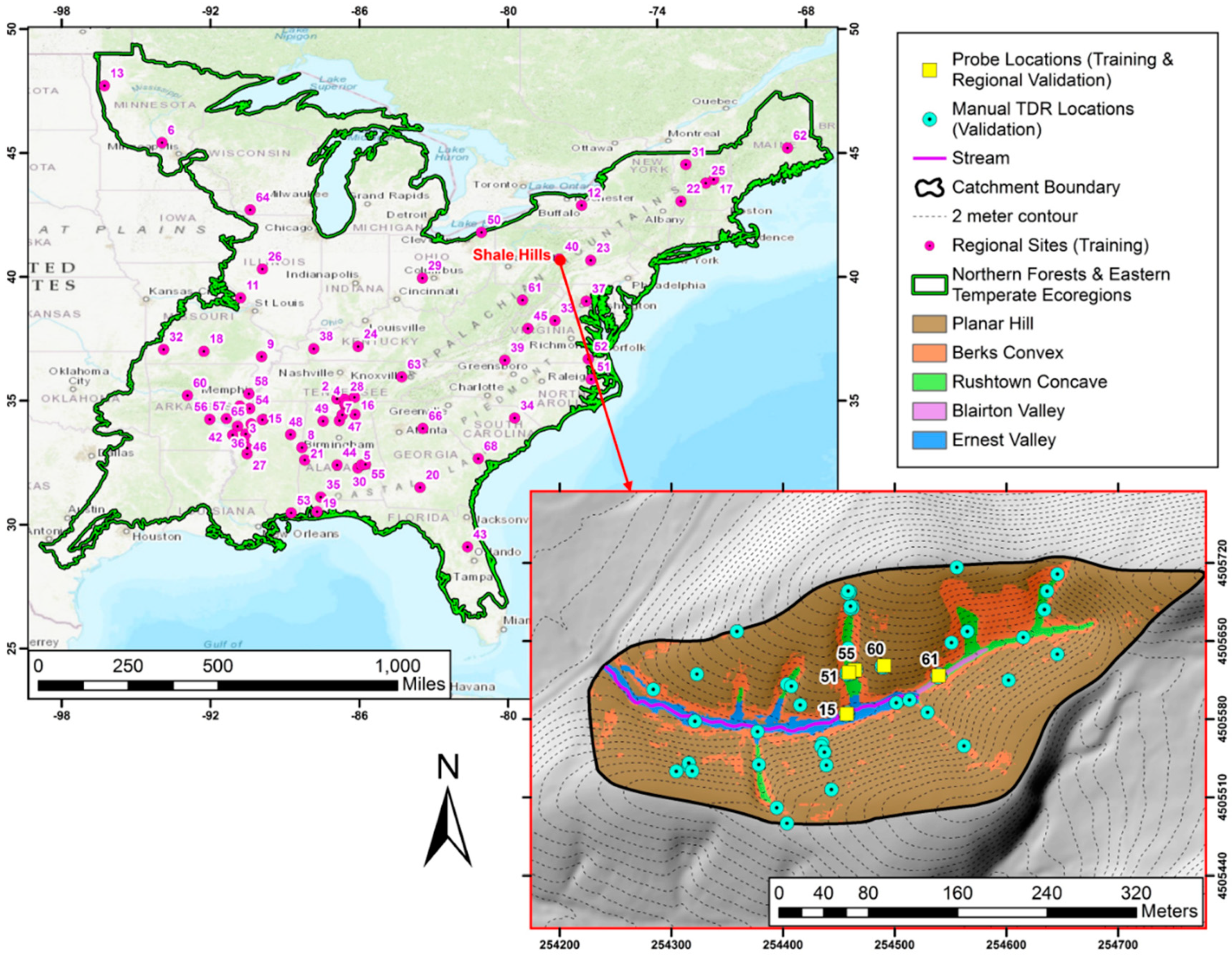
2.1. Study Areas

Data from the Shale Hills research catchment was first used to address our first research question. The Shale Hills Catchment is a 7.9 ha forested watershed characterized by steep slopes (from 25%–48%) and narrow ridges. The catchment valley is oriented in an east–west direction, and has an elevation ranging from 256 to 310 m above sea level. Lin et al. [46] identified five soil series in the catchment. The Weikert series (loamy-skeletal, mixed, active, mesic Lithic Dystrudept) is the predominant soil type in the catchment, comprising 78% of the area and is characterized as a thin soil on hilltops, planar, and convex hillslopes. The Rushtown series (loamy-skeletal, over fragmental, mixed, mesic Typic Dystrochrept) is mostly located in the center of the four dominant concave hillslopes and the majority of the upper 100 m of the main catchment valley. The Berks series (loamy-skeletal, mixed, active, mesic Typic Dystrudept) is well-drained and largely distributed along the slope transitional zones between the shallow Weikert and the deep Rushtown soils. The Blairton series (fine-loamy, mixed, active, mesic Aquic Hapludult) is located in the valley bottom, with an argillic horizon at a 0.2 to 0.8 m depth and few (2%–5%) redox features starting at a 0.8 to 1.1 m depth. The Ernest series (fine-loamy, mixed, superactive, mesic Aquic Fragiudults) is a deep (>3 m depth to bedrock), poorly to moderately well-drained soil on the valley floor with many redox features. The Ernest valley soil surrounds a first-order stream that is active typically from mid-November to the beginning of June. A 110-year-old mixed forest dominated by an oak (Quercus spp.), maple (Acer, spp.), hickory (Carya, spp.), and eastern hemlock (Tsuga canadensis, spp.) canopy covers the entire catchment. The annual precipitation is 900 mm and the mean annual temperature is 11 °C. Figure 1 displays the catchment in an inset with the calibration and validation monitoring locations we used in this study.
The Shale Hills lies in the Eastern Temperate Forest Level 1 ecoregion, following the spatially hierarchical ecoregion delineation designed by Omernik [47]. Ecoregions are defined by regions with similar climate, vegetation, and terrain at different scales, Level 1 being the broadest. Past efforts have shown that SMAR can be adequately calibrated in regions that are not semi-arid, such as the Eastern Temperate Forests, and that the over- or under-estimation (i.e., bias) of satellite data products relative to near-surface in situ soil moisture measurements are similar within Level 1 ecoregions [41]. This study pursues a more direct approach to SMAR calibration, where ecoregion-level satellite bias was not estimated outside of the SMAR model optimization process.
The regional-scale SMAR model was calibrated and tested across the Eastern Temperate Forest and Northern Forest ecoregions to address our second research question. We limited our regional scope to these two adjacent Level 1 ecoregions within the United States, since they have a relatively dense amount of in situ soil moisture monitoring sites and coverage of soil property maps (Section 2.3). The general over- and under-prediction of near-surface soil moisture by satellite data products relative to in situ measurements is expected to differ between these two ecoregions [41], however, applying this RZSM mapping approach across different ecoregions is a test of its overall robustness. Note, the Eastern Temperate Forests and Northern Forests include most of the United States area east of the Mississippi River and are not limited to just forest land cover, as the names imply.

2.2. In Situ Data for SMAR Calibration and Validation

In the Shale Hills and regional EUS SMAR modeling test cases, both in situ root zone soil moisture and satellite data products were involved in the SMAR model training or calibration. A different set of in situ soil moisture data was set aside from being used for calibration to validate the SMAR model in both test cases.
The Shale Hills is a densely instrumented catchment with a temporally and spatially rich collection of soil moisture monitoring data. Automatic volumetric soil moisture (cm3 cm−3) measurements were collected from five monitoring locations in the catchment with Decagon ECH20 probes at multiple depths (yellow squares in Figure 1). Each probe has a spatial resolution of 0.02 cm3 cm−3 and measures soil moisture every 10 minutes. To match the temporal resolution of the SMAR infiltration model and satellite forcing data, the 10-minute soil moisture measurements are aggregated into a daily value (i.e., 24-hour) by averaging all measurements in each 24-hour period. Soil texture and porosity were required for initial parameter estimates and the calculation of RZSM, and Lin [48] provides soil texture data for each probe used in this study. We used pedo-transfer functions [49] to derive estimates of porosity from soil texture [40] for each probe within each monitoring location. We estimated the relative soil moisture by dividing soil moisture into porosity. Relative root zone soil moisture at a location was then taken as the mean of all relative soil moisture values from probes below the probe closest to the surface (see Manfreda et al. [40] for a discussion on near-surface delineation for SMAR modeling).
A separate dataset of manually collected volumetric soil moisture measurements is available for validating spatial SMAR estimates of RZSM at Shale Hills. These data were collected bi-weekly since 2005 with a TRIME-FM hand-held time-domain reflectometry (TDR) probe [50] at locations indicated by the cyan colored points on the Shale Hills map in Figure 1. The manual TDR probes were inserted at 10-, 20-, 40-, 80-, and 100-cm depths at up to 65 locations, and their spatial distribution represents each soil type and soil-terrain unit in the catchment (see Lin [48] for further data collection details). Manual TDR soil moisture content data was converted into RZSM in the same manner as the 10-minute probes: All measurements was divided into soil porosity and RZSM is the mean of the values from all depths, given that the top depth of 10 cm is within the ‘root zone’. The manual TDR RZSM data was collected once at each location within each sampling date.
A regional network of 68 unique in situ monitoring sites offers data for the calibration of regional SMAR (Table S1; purple points in Figure 1). Sixty-five of these sites were taken from the soil climate analysis network (SCAN; [11]) and three sites from the North American Fluxnet (AMERIFLUX) network [51,52,53]. We followed the same approach for aggregating in situ measurements from the AMERIFLUX network into daily RZSM as the automatic sensors in Shale Hills, where half-hourly measurements were averaged into daily values; SCAN data was downloaded in averaged daily form directly. All measurements below the top 5 cm depth were then averaged into one ‘root zone’ moisture content value, and then this averaged value was converted into the relative RZSM by dividing into root zone porosity for a given site. Root zone porosity for each site was estimated from applying CONUS soil texture data [54] (Section 2.3) with the Rawls et al. [49] pedo-transfer function, since CONUS soil property data is available across the region and not all sites have available soil texture information. The root zone porosity estimated by soil texture is too low at some sites, where a significant portion of the converted RZSM values are >1. Therefore, root zone porosity was adjusted upwards slightly until at least 95% of RZSM values were <1. Figure S1 shows the time-series of volumetric root zone soil moisture from each site selected for calibrating regional SMAR, as well as corresponding satellite near-surface data from all three platforms. Table S1 gives the temporal range selected for each site’s calibration period and associated root-zone porosity values.

2.3. Catchment Stratification and Regional Soil Property Maps for SMAR Spatial Operation

In both the Shale Hills and EUS region SMAR modeling test cases, spatial soil property information was used to assign or estimate SMAR parameters across space for its spatial operation (Section 2.5).
Variables derived from a light detection and ranging (LiDAR) survey are used for the catchment stratification of Shale Hills, and this stratification supports the spatial operation of SMAR within Shale Hills by parameterizing the spatial model according to similar areas of soil physical properties. Terrain variables calculated from a LiDAR-derived DEM [55] were integral in the formulation of up to five ‘soil-terrain’ map units that comprise a stratification of the catchment into areas of similar physical soil and topographic properties. The LiDAR data was processed with TerraScan software, which classifies raw LiDAR point data, and the ground points were interpolated across space using ordinary kriging to create the DEM. A Gaussian filter was applied with a 4.5 × 4.5 m smoothing window to reduce noise in the DEM. The terrain variables derived from the DEM used in the soil–terrain delineation are the topographic wetness index, surface curvature, log-transformed upslope contributing area, vertical distance to stream channel, and local slope. A map of the depth to bedrock was also important in delineating these soil–terrain units, and the depth to bedrock map was generated by interpolating augur point measurements with regression kriging [56] using LiDAR-derived terrain variables, such as the topographic wetness index and surface curvature, as covariates. Each of the five soil–terrain units had a corresponding automatic soil moisture monitoring location.
The CONUS soil property maps developed by Miller and White [54] are 1-km resolution maps of soil physical properties over multiple layers at uniform depth intervals based upon the State Soil Geographic Database (STATSGO). We used these maps to estimate porosity at SCAN/AMERIFLUX sites, extrapolating root zone field capacity across the EUS study region with the Rawls et al. [49] pedo-transfer function, and used them as covariates for estimating calibrated SMAR model parameters. A ‘root zone’ equivalent for each soil property was derived by averaging values from all layers beneath the top-most layer at each CONUS soil map pixel, and specifically, we used soil textural fractions (clay, sand, silt %), bulk density (g cm−3), porosity (cm3 cm−3), and depth to bedrock (m). Additionally, a 100-m resolution DEM was used as another covariate in SMAR parameter estimation [57], which was resampled to 1 km to match the CONUS soil grid. Figure S2 reveals that the 68 ground-based sites are representative of the soil texture, according to the full CONUS dataset for the EUS region.

2.4. Satellite Remote Sensing Data

We used NASA’s Advanced Microwave Scanning Radiometer (AMSRE) satellite Level 3 data product [58], the European Space Agency’s Soil Moisture Ocean Salinity (SMOS) Level 2 data product [59], and NASA’s Soil Moisture Active Passive (SMAP) Level 3 passive data product [60] as near-surface soil moisture input data for SMAR. These satellite platforms use a passive microwave sensor to observe the intensity of microwave emissions from the thin, near-surface soil layer (0–2 cm depth). The microwave emissions are directly related to the product of surface temperature and surface emissivity, or ‘surface brightness temperature’ [61]. The AMSRE data product (25-km resolution) was ideal for our study because of its relatively long data record (2002–2011) and overlap with Shale Hills’ automatic and manual soil moisture datasets. We used AMSRE soil moisture retrievals by the X-band to avoid problems associated with radio-frequency interference from urban areas that affect the C-band or 6.92 GHz channel. Specifically, the AMSRE soil moisture data product used here is derived from the land parameter retrieval model algorithm [62], which considers potential bias from surface roughness and vegetation canopy. The SMOS Level 2 data product (15-km grid resolution) utilizes multi-angular observations of brightness temperature to retrieve both soil moisture and vegetation optical depth, with an average 40-km spatial resolution at the L-band frequency [59]. Retrievals from the L-band occur at a slightly deeper depth than those from AMSRE. The SMAP Level 3 passive data product is a daily composite of global soil moisture retrievals based upon the L-band microwave frequency, as well, and we used the ‘enhanced’ soil moisture passive product from SMAP, which provides retrievals at a 9-km spacing.
We took the mean of the soil moisture data product derived from daily ascending and descending passes of each platform as our near-surface soil moisture estimate to accommodate the daily time-step of SMAR. This has been applied in past studies that use daily AMSRE data as a model forcing [63]. Data gaps exist in the SMOS and SMAP data products’ time-series in areas prone to extended snow cover and dense vegetation. We addressed relatively short, up to week-long temporal gaps, with a linear imputation for affected pixels [64], but gaps more than a week remained as missing data. The SMOS and SMAP data products required normalization into relative near-surface soil moisture for use in SMAR, and we adopted a piece-wise linear function to normalize near-surface soil moisture, based upon the concept of ‘effective soil moisture’ in past studies [65]:
S 1 = ( θ o b s   θ m i n ) ( θ m a x   θ m i n ) ,
where S1 is the relative near-surface soil moisture, θobs is the volumetric soil moisture content (cm3 cm−3) retrieved by SMOS and SMAP platforms, and θmaxmin is the maximum/minimum soil moisture value retrieved by these platforms. This approach assumes that θmax approximates near-surface saturated moisture content, which may be a safe approximation across the multi-year time-series of SMOS and SMAP retrievals in that surface-saturating precipitation events have most likely occurred during this time period. The normalization method enabled the SMOS and SMAP data records to scale similarly with the already-normalized AMSRE Level 3 data (Figure S1).

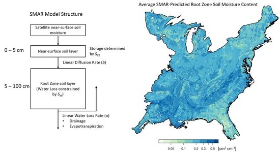
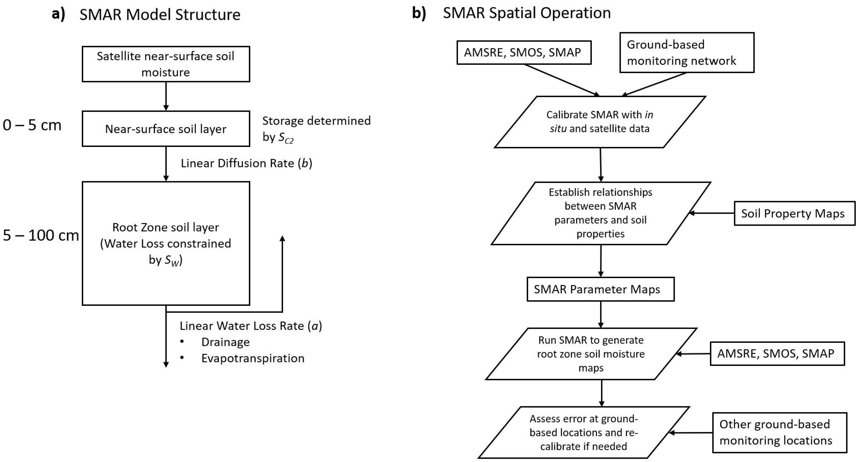
2.5. SMAR Model Formulation and Spatial Operation

The SMAR model simulates the diffusion of moisture from a near surface layer (0–5 cm) into the root zone (5–100 cm), as well as the soil water losses out from the root zone at a daily time-step. The amount of water available to enter the root zone (y) is equal to the water content exceeding a relative saturation value representing near-surface field capacity (SC1). Water loss is a function of root zone leakage in all SMAR model versions, but a non-linear version of SMAR incorporates evapotranspiration (ET) into the water loss function. A temporally discrete form of the SMAR model is:
S 2 ( t i ) = [ S W + ( S 2 ( t i 1 )   S W )   e x p a ( t i t i 1 ) ] + [ ( 1 S W ) b   y ( t i ) ( t i t i 1 ) ] ,
where a is a fitted parameter (days−1) representing normalized daily root zone water loss, b is a fitted parameter (-) controlling the diffusion rate of excess moisture (y) into the root zone (“diffusivity coefficient”), SW is the root-zone relative wilting level (-), and S2 (-) is the relative root-zone moisture content at time t (i.e., RZSM). The water loss (a) parameter (day−1) determines the rate at which the water loss function decreases with S2(ti−1) until SW is reached. The water loss parameter is taken as a daily leakage rate V (cm day−1) normalized by the soil root zone thickness (Z2), root zone porosity (ρ2), and SW:
a =   V ( 1   S W )   ρ 2   Z 2 .
For the SMAR spatial operation across Shale Hills, each soil–terrain landscape unit was assigned calibrated SMAR parameter estimates. The spatial assignment of the water loss coefficient (a) is more complex than SC1, b, and SW, since the Shale Hills depth to bedrock map provides a higher resolution spatial variation of the root zone thickness (Z2) across the catchment than ρ2 (root zone porosity is the same for each soil–terrain unit): The coefficient, V, was back-calculated from the calibrated parameter, a, at each monitoring location by rearranging Equation (3) and using the location’s root zone thickness and porosity. Then, the a parameter was further varied across space by using Equation (3) with a map of depth to bedrock (1-m resolution). The depth to bedrock map is limited to 100 cm at the deepest, which is the maximum assumed root-zone thickness in this study. The AMSRE near-surface soil moisture time-series from 2007 to 2011 was used as a forcing dataset for the Shale Hills experiment, since large gaps occur in SMOS across the available Shale Hills automatic time-series record from 2011 to 2012.
A similar approach was used to operate SMAR across space at a regional level, where soil property data was used to assign parameters to a 1-km model grid with the same structure as the CONUS soil property maps. The SMAR model was optimized to RZSM from 68 sites across the EUS region, excluding Shale Hills, and a different set of SMAR parameters were estimated for each available satellite platform. A site must have at least 2 years of in situ RZSM data that overlaps with a satellite platform’s time-series, which must also not have significant time gaps (>2 months). These optimized parameters were then related to CONUS soil property maps to generate SMAR parameter maps corresponding to each satellite platform for the EUS. The SMAR model was initialized by the root zone field capacity, estimated through soil texture taken from sand, silt, and clay textural fraction data from CONUS and Rawls et al. (1993). The relative near-surface soil moisture grids from AMSRE, SMOS, and SMAP were then resampled to the resolution of CONUS soil (1-km) using a nearest neighbor routine, and this grid was used to force the gridded spatial SMAR model. Table 1 lists all datasets and SMAR parameters used in this study.
We used neural network models to relate calibrated SMAR parameters to CONUS soil property variables for the regional implementation of SMAR. Three sets of maps were created for each SMAR parameter, after optimizing them at 68 unique locations with varying availability for AMSRE, SMOS, and SMAP satellite data. Multiple linear regression was used to predict fitted SMAR parameters with soil properties [41], but this was used with parameters predicted with in situ data only, where a more direct physical relationship between SMAR parameters and soil properties was expected. The relationship between SMAR parameters estimated with satellite data and CONUS soil properties is more complex, because of the scale discrepancy between these data and point-based measurements.
Neural networks have been trained to accurately predict soil hydrologic properties with soil physical properties [45], and they are a useful predictive tool that can account for complex and ‘hidden’ error structures that may be present in a model [66]. We trained a neural network algorithm using a resilient backpropagation algorithm to minimize the sum of squared errors [67,68] to predict each SMAR parameter from each satellite platform with near-surface and root-zone CONUS clay, silt, and sand textural fractions, bulk density, porosity, elevation, and depth to bedrock. The CONUS root-zone porosity layer is a separate porosity layer from the estimated root-zone porosity calculated with Rawls et al.’s [49] function. Additionally, the USGS elevation [57] was used as another covariate along with soil properties in the neural network. We specified two hidden layers in the neural network model with a total of eight hidden neurons. All independent variables were scaled prior to neural network model-fitting by subtracting the mean and dividing by the standard deviation. These same means and standard deviations were used to scale the CONUS data for the entire EUS region, which was used to create regional maps of SMAR parameters with the fitted neural network models.
Evaluating the interactions of all independent variables to each dependent SMAR parameter is out of this study’s scope, so we did not conduct a sensitivity analysis on these neural networks. Our objective was to generate the best possible predictive model with the full set of SMAR parameters for each platform, so we gauged neural network accuracy by evaluating the observed versus predicted SMAR parameters from all sites. Although we expected some multi-collinearity between independent variables, a visual inspection of maps for all near-surface, root zone, and other soil properties used as predictors did not reveal a pair that was overwhelmingly correlated to each other across space. A robustness test of the use of these neural networks to predict SMAR parameters was conducted by gauging the actual predictive accuracy of spatial SMAR (Section 2.6), rather than focusing on potential over-fitting of the neural network models.
In summary, the SMAR model receives satellite near-surface soil moisture and outputs estimates of the root-zone soil moisture. The overall model structure is a relatively simple ‘soil bucket’ modeling approach, and the model operates with relative soil moisture variables (i.e., volumetric soil moisture divided by porosity). We used spatial soil physical property and terrain data to map SMAR parameters across space, which facilitated the spatial operation of SMAR. The spatial operation of SMAR was first tested at Shale Hills, where map units representing areas of similar soil physical properties were used to assign SMAR parameters across space. Next, a regional-scale SMAR was tested, and maps of SMAR parameters for the EUS region were created with CONUS soil physical soil data. A schematic of the SMAR model structure and the general spatial SMAR routine are given in Figure 2a–b.
We created multiple datasets with the spatial SMAR model operation in this study. The first is a time-series of catchment-scale maps of RZSM, produced by the Shale Hills specific SMAR model. Second, we created regional SMAR parameter maps that are specific to each satellite platform (AMSRE, SMOS, and SMAP), with CONUS soil and USGS elevation data inputted into trained neural networks. Finally, we generated three separate time-series of EUS regional RZSM maps using the regional SMAR model with inputs from the three satellite near-surface soil moisture data products. All outputs are listed in Table 2.

2.6. SMAR Model Calibration and Validation

Soil moisture datasets associated with Shale Hills and the EUS region are used for either training, validation, or both purposes. A RZSM training dataset for estimating optimal SMAR model parameters in Shale Hills at the five automatic monitoring locations is a continuous record from 2009 to 2011 (yellow squares in Figure 1). These years provide a near continuous stream of RZSM data for each location with relatively few data gaps, no longer than 2 months at most. We used the independent manual TDR dataset (cyan points in Figure 1), which was collected during this time-period, to validate the spatial SMAR soil moisture maps in Shale Hills. The SCAN/AMERIFLUX datasets (purple points in Figure 1) were used to estimate a set of SMAR parameters for the AMSRE, SMOS, and SMAP platforms for the regional SMAR operation. Finally, the automatic monitoring locations at Shale Hills (yellow squares in Figure 1) were used to validate the EUS regional SMAR model, since this data was not used to train the regional SMAR model. All SMAR parameters in this study were optimized with the same approach.
Model parameters were optimized by assimilating near-surface satellite data and in situ RZSM data within a hierarchical Bayesian framework. A normal negative log-likelihood objective function was minimized by the algorithm during the fitting process, and posterior probability distributions for each SMAR parameter (i.e., SC1, a, b, SW) were approximated. Before running a Monte Carlo Markov chain (MCMC) algorithm, a Levenberg–Marquardt derivative-based algorithm [69] estimated optimal parameters from the same training dataset used by the MCMC algorithm. An adaptive MCMC algorithm with a delayed rejection [70] simulated potential parameter values from a range of physically meaningful values, and proposed parameter values were rejected if their acceptance ratio was less than one. Three MCMC chains were run for each optimization procedure, where one of the MCMC chains was initiated by the Levenberg–Marquardt estimates, while the second chain was initiated by half of the Levenberg–Marquardt estimates, and the third chain was SMAR values predicted by soil texture and Rawls et al. [49]. The relatively disperse initial MCMC chain settings across the three MCMC chains enabled a relatively wide sampling of the range of physically possible values for each SMAR parameter at each monitoring location. We assigned a uniform prior distribution for each model parameter that covers the range of physically possible values for each parameter, assumed to be 0 to 1 for all parameters and locations besides the SMAR water loss (a) parameter for the planar hillslope location at Shale Hills, which undergoes relatively fast drainage of moisture downslope. Measurement error was assumed to follow a normal distribution, with variance as σ p 2 . The σ p 2 is a nuisance parameter with an initial value assigned at the start of the MCMC procedure that is the model variance associated with the Levenberg–Marquardt model fit.
We applied the Gelman–Rubin test [71] to determine whether all MCMC chains converged upon the same stationary parameter space after the optimization was complete. The mean of each posterior probability distribution represents the final parameter estimate. We used the MCMC algorithm in the R package ‘FME’ [72] and the MCMC results were analyzed with the ‘coda’ package [73].
A, RMSE of 0.06 cm3 cm−3 has been taken as a benchmark of acceptable model performance when using AMSRE data to predict near-surface soil moisture [43,44], so we analyzed where each model meets this benchmark across the Shale Hills catchment. Given that only 68 sites met any criteria for training the EUS regional SMAR, a thorough validation could not be conducted across the EUS region. However, the automatic sensors at Shale Hills were used to validate the regional EUS SMAR maps for Shale Hills alone, since they were excluded from the regional SMAR model training and provide a continuous time-series of soil moisture data. We did get a sense on how initial conditions may affect the regional SMAR model accuracy, since the model optimization at EUS sites was initialized at that site’s first RZSM measurement, while the regional SMAR model was initialized at the beginning of each satellite platform’s time-series. The initial data of each satellite’s time-series was always earlier than the initial date of the in situ training datasets used to estimate EUS parameters.
Given the multi-year validation dataset at Shale Hills, we analyzed whether the validation RMSE exhibits a temporal pattern and evaluated whether spatial SMAR consistently under- or over-predicts RZSM with a mean bias metric at Shale Hills. We quantified mean bias as:
B i a s =   y ¯ [ i = 1 n y ^ i / n ] ,
where y ¯ is the mean of observations within a soil–terrain unit or throughout the entire catchment, n is the number of predictions, and y i ^ is a model prediction at a certain spatial level (i.e., specific soil–terrain unit or catchment) at time-step i. If an SMAR model is under-predicting on average, the result of Equation (4) will be positive, and it will be negative if an SMAR is over-predicting on average. We evaluated RMSE for model performance across quarters of the year (i.e., quarter 2: April–June; quarter 3: July–August; quarter 4: September–November).
The root-zone soil moisture maps outputted during this research and example code may be downloaded at: https://github.com/dcb5006/SMAR_EUS_RemoteSensing. Also, all materials, data, computer code, and protocols associated with this publication are available to readers upon request.

3. Results

Our results are organized into two sections, each devoted to one of our two research questions, where question one focuses on testing SMAR at a catchment-scale and question two focuses on testing SMAR at a regional-scale. Each section presents results as they relate to operating the spatial SMAR model with near-surface satellite data, as explained in Section 2.5. The outcomes of the calibration and validation procedures described in Section 2.6 are also explained in each Results section, which answers both research questions.

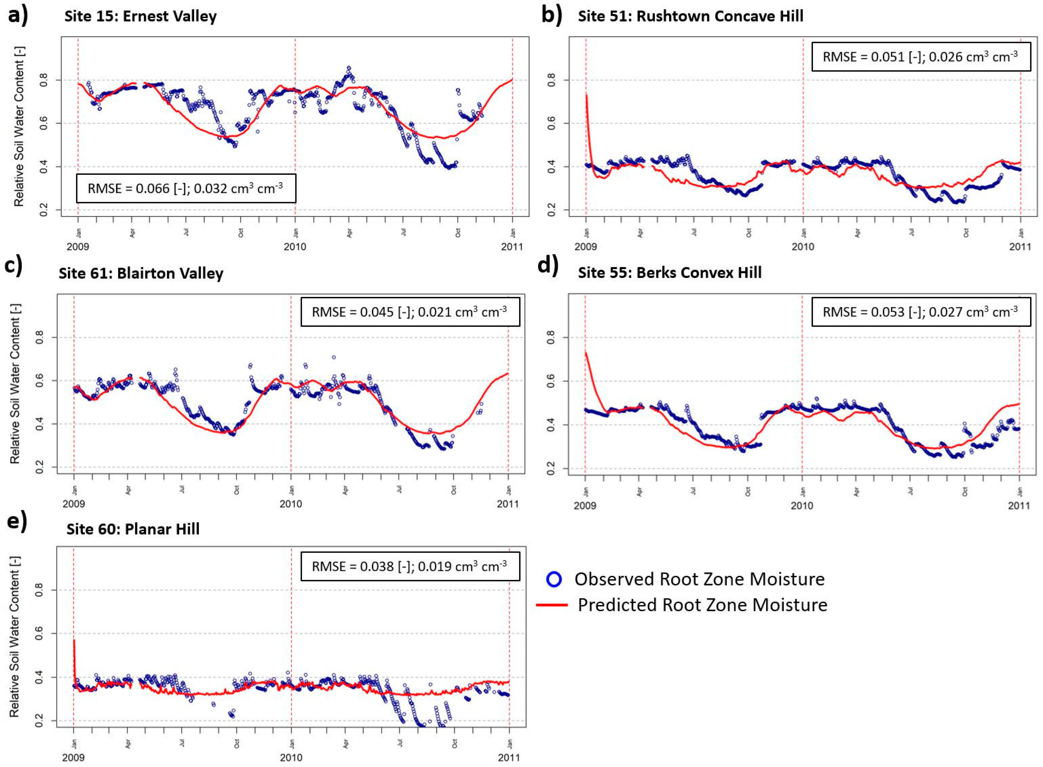
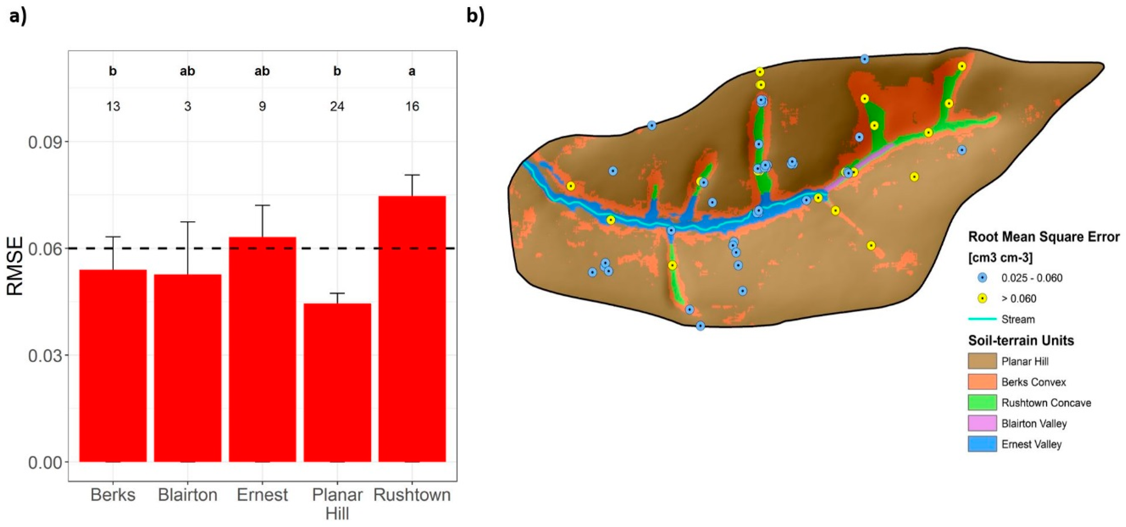
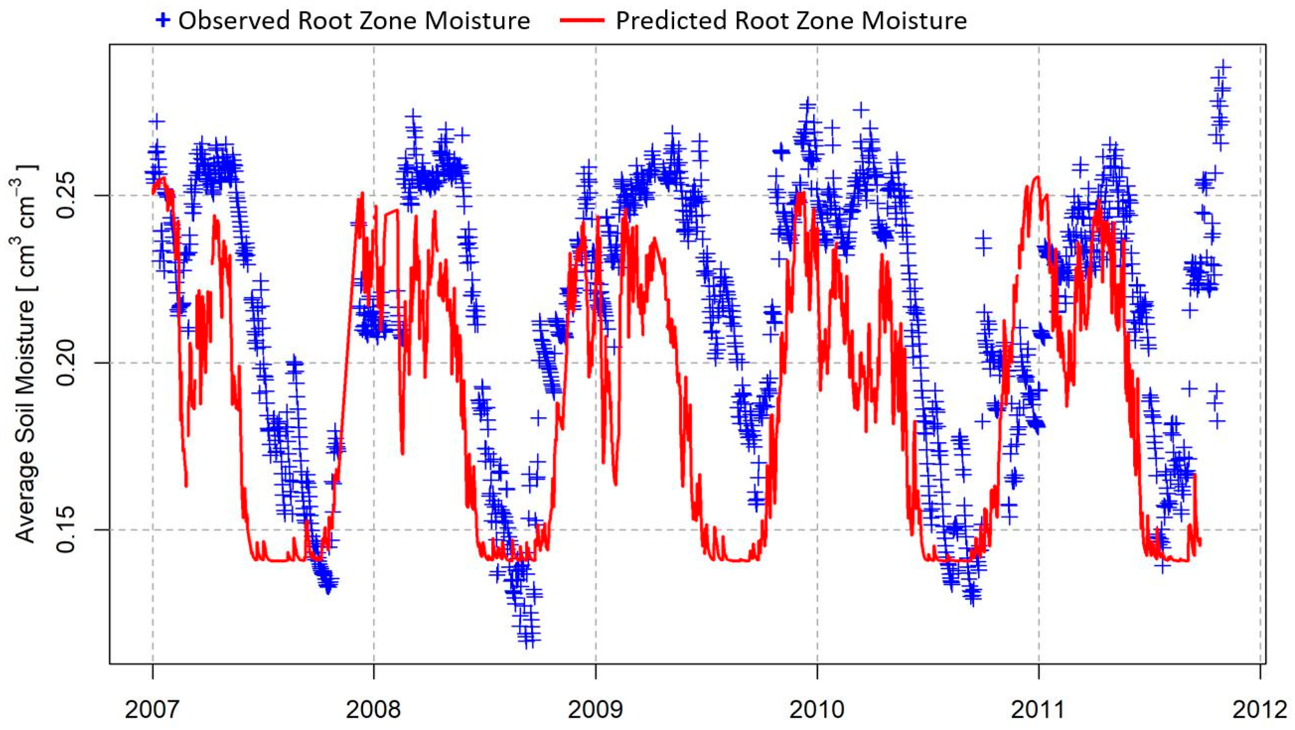
3.1. The Shale Hills Catchment

Results presented in this section address research question one (how accurate is a spatial SMAR across different soil types and landforms in Shale Hills after being calibrated to data at select locations in the catchment, and where does it do best?). The SMAR model provides reliable model estimates of root-zone soil moisture after calibration when compared to measurements at all training locations. The validation results show that the relatively simple SMAR model is reliable at providing adequate predictions for all soil–terrain units but the concave hillslope unit. It meets the RMSE benchmark at the relatively wet Blairton valley unit and the dryer planar hillslope soil, which dominates the catchment. SMAR’s accuracy drops during the ‘dry-down’ period of April to June at Shale Hills.
The three MCMC chains converge and fluctuate in a stable parameter ‘space’ (or range of values) for each SMAR parameter during the model optimization at the Shale Hills, given by Gelmin–Rubin statistics that are close to 1 for each parameter at each site (Table S2). The RMSE estimated upon comparing predicted volumetric RZSM are all <0.06 cm3 cm−3, indicating relatively close model agreement to observations (Table S3). Figure 3a–e reveal the observed and predicted RZSM at each training site, including the predictions during model ‘spin-up’, directly after the initialization. The influence of initial conditions, which were set at the estimated root zone field capacity, fade after about 2 months for all sites. The model can capture general episodes of wetting and drying in the root zone at most sites, which is a critical requirement for satellite-derived soil moisture products. Notably, the Planar Hill site shows close agreement between SMAR predictions and observations during wetter periods, but the model cannot capture the substantial release of moisture during dry periods on this hillslope.
Table S3 lists optimal parameter estimates for each model. Near-surface field capacity (SC1) is higher on the hillslope areas than the two valley sites, indicating that less near-surface moisture is released into the root zone at these sites. The relative root-zone wilting level (SW) is highest at the wettest Ernest valley site (S15) but is also relatively high on the planar hillslope. Diffusion (b) is similar across all sites, given that the range of values is small among the five sites compared to the range of typical diffusion values (i.e., 0–0.50 (-)). The highest water loss (a) occurs at the shallow and moderately steep soils of the planar hillslope (S60), where the normalized water loss rate is greater than 1 day−1. Water loss is also relatively high at the Rushtown concave hill site.
An evaluation of RMSE from validation of spatial SMAR with manual TDR data reveals that error is generally highest at the Rushtown concave hillslope (Figure 4a). Almost all validation sites show an RMSE >0.06 cm3 cm−3 in the green Rushtown concave hillslope patches in Figure 4b. The 0.06 cm3 cm−3 RMSE benchmark is maintained throughout 80% of the Planar Hillslope, which is apparent from the points in Figure 4b across the planar hillslope area; points close to the ridge top on soil at the north-central portion of the catchment register RMSE > 0.06 cm3 cm−3. In total, 66% of all locations throughout the catchment meet the RMSE benchmark for validation. Based upon the spatial patterns of RMSE (Figure 4), SMAR predictions are generally closer to soil moisture observations in soils outside of concave swales and in central and western areas of the catchment.
Model error is generally higher during quarter 2 (April–June) for the SMAR model at each monitoring location (Table 3), the highest being at the Rushtown concave hill. The only site that increased in error during Q3 to Q4 compared to Q2 is the Ernest valley. The planar hillslope is the most consistent error-wise throughout different times of the year, with the dryer Q3 period being a bit higher than others. The planar hillslope is the only area where SMAR consistently over-predicts volumetric soil moisture data, and it does so to a larger degree during Q3. There is not enough data for quarter 1 (Q1) to make any meaningful summary or comparisons, but Q1 data did make up the annual RMSE metric. The addition of Q1 data made the overall RMSE average higher at the Ernest valley site.

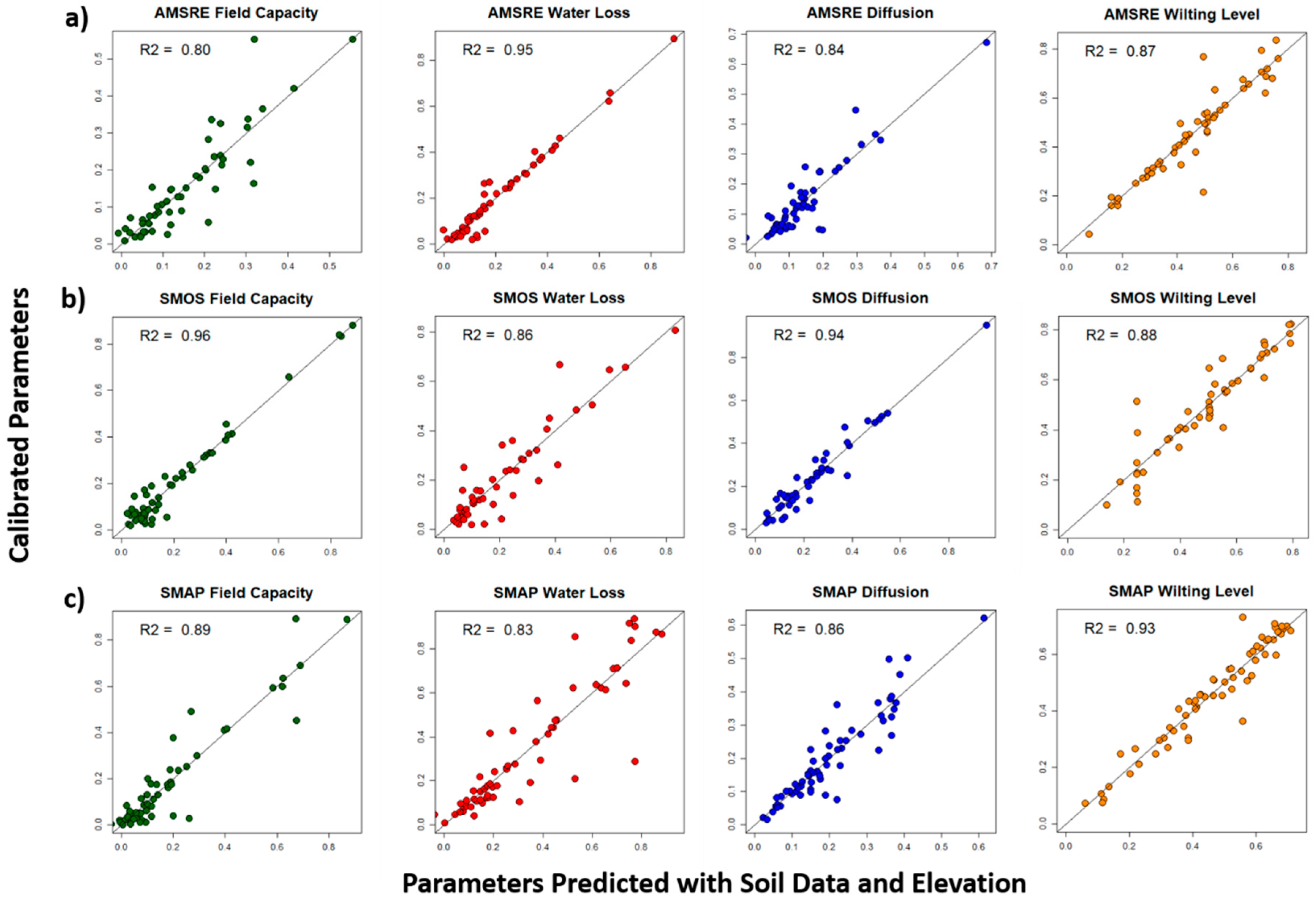
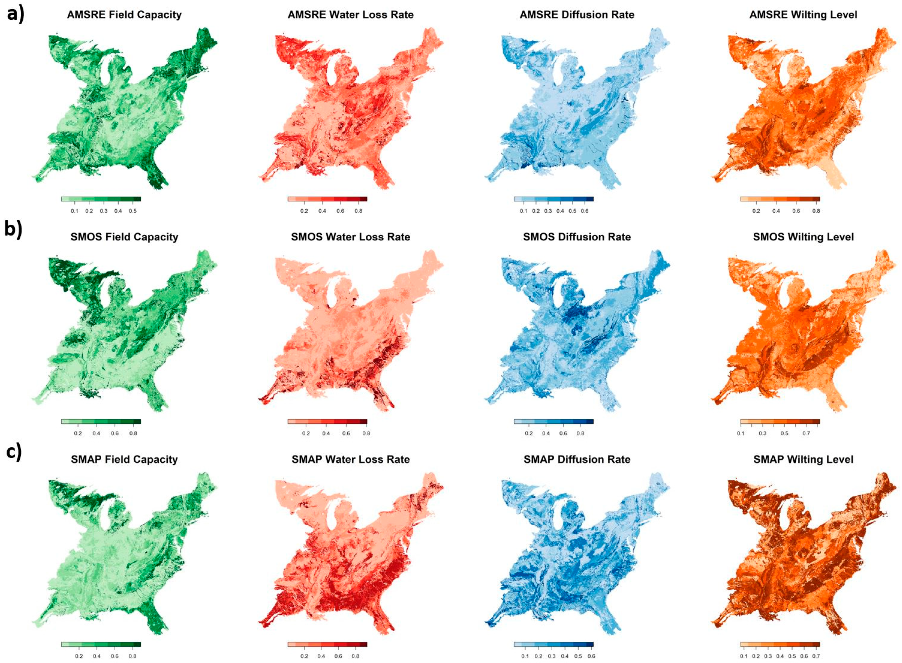
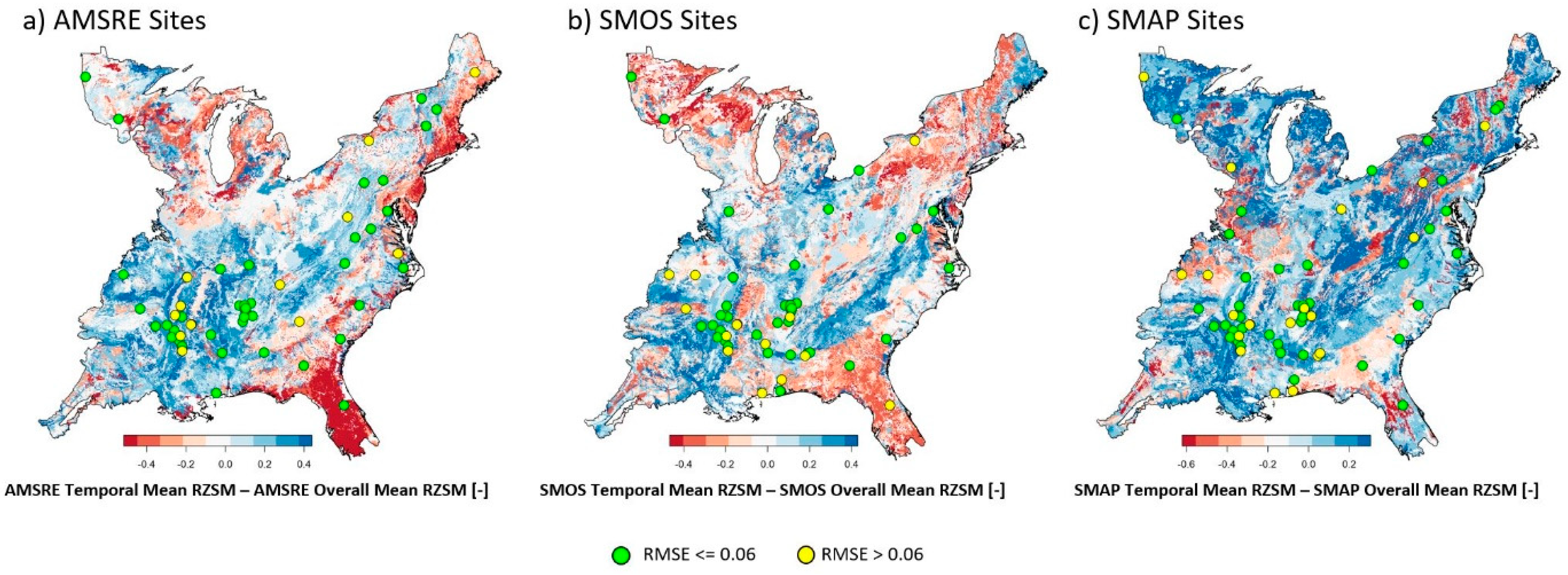
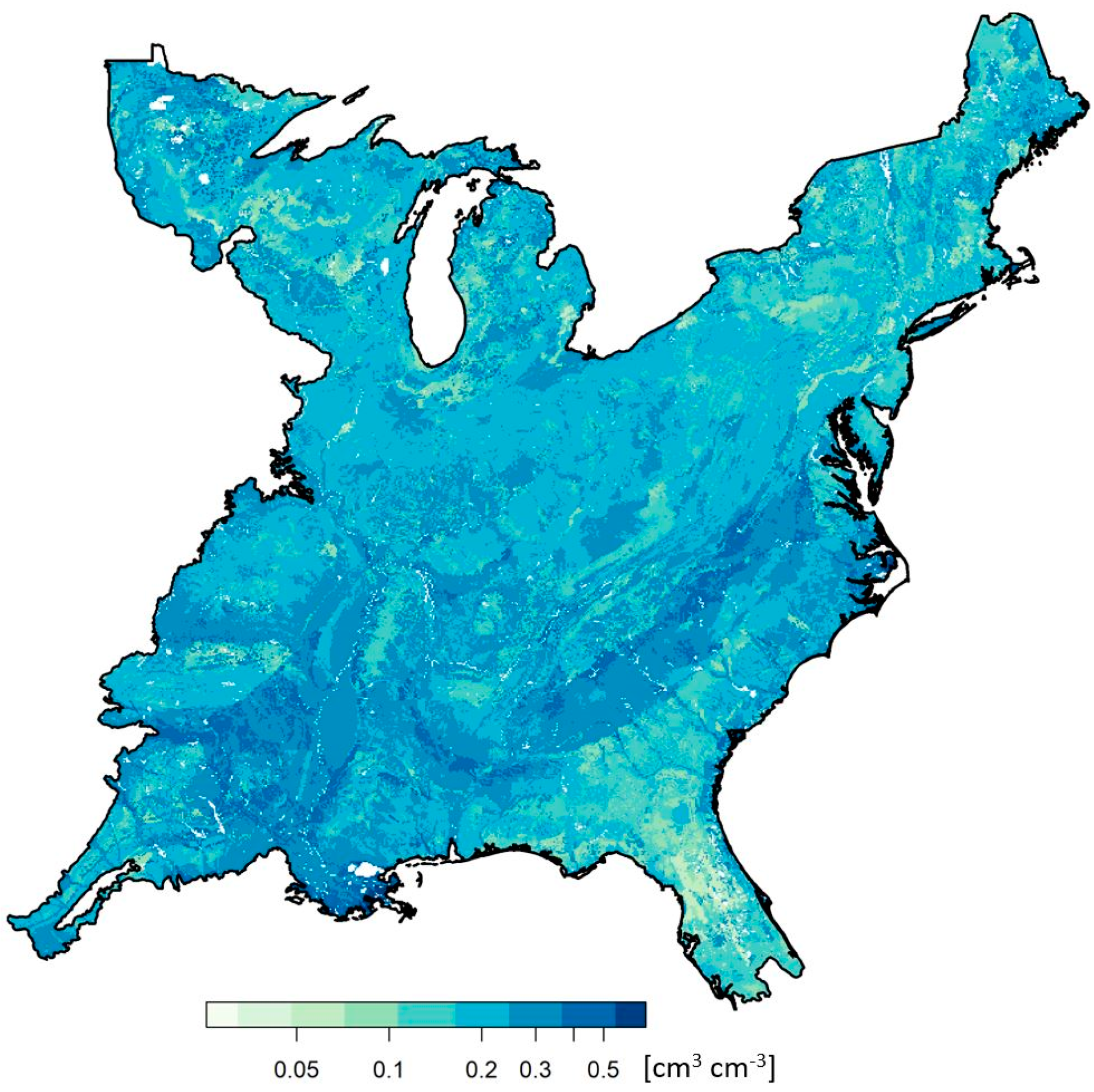
3.2. The Eastern United States Region

Results from the following section answer the second research question: Can SMAR parameters that are optimized directly with three different satellite data products be mapped at a regional extent with soil properties and be used to run a spatial SMAR that provides an adequate level of accuracy on average? Calibrated SMAR parameters can be predicted with the use of a contemporary neural network algorithm, and on average, the regional SMAR can meet a quality benchmark of RMSE <= 0.06 cm3 cm−3 on average at a site-level if accurate soil porosity information is available for that area.
The optimization analysis converged on stable parameter spaces for SMAR parameters at all sites for each satellite platform (Table S2), in that all Gelmin–Rubin statistics are <1.1. The average SC1 is similar across different satellite platforms, with near-surface field capacity being slightly higher on average for SMOS and SMAP compared to AMSRE (parameters listed in Table S3). Water loss (a) is higher on average for SMAP compared to the other platforms, and both SMOS and SMAP have higher diffusion rates (b) than AMSRE. The relative root-zone wilting level (SW) is similar across all platforms. A multiple linear regression did not provide satisfactory results when using CONUS soil properties to predict SMAR predictors for all parameters (data not shown); however, root-zone sand content had a highly statistically significant (p < 0.001) and negative association with log-transformed SW across all three satellite platforms, indicating that areas with high sand content tend to release more moisture from their root zone during dry periods than areas with low sand content.
The trained neural network did a fine job at predicting SMAR parameters across all three satellite platforms with the scaled CONUS soil data (Figure 5a–c). The neural network models reveal no predictive bias or any serious heteroscedasticity in their predictive error for any parameter across all platforms. The neural networks that predict SMAR parameters from SMOS and SMAP data show higher R2 values than those from AMSRE for all SMAR parameters but water loss (a). Notably, the neural network accuracy declined when the USGS elevation was not included, indicating elevation is an important covariate to include along with CONUS soil properties for estimating spatial patterns of SMAR. In total, the variables used in the neural network model to predict each SMAR parameter map are the elevation; surface and root-zone clay, sand, and silt content; and the surface and root-zone porosity and bulk density.
The regional SMAR parameter maps derived from the neural network models and CONUS soil/USGS elevation data reveal some similar spatial patterns across different satellite platforms for SC1, b, and SW parameters (Figure 6a–c). Near surface field capacity tends to be high in the southeast and northwest part of the region for all satellite platforms, but AMSRE also shows relatively high values in northern New England forests that contain silt loam and silty clay loam near-surface soils, per CONUS soil data (Miller and White, 1998). Diffusion (b) is more pronounced in central areas of the region for each platform that correspond with higher root-zone clay and silt textures. Diffusion is consistently lower in the southeast for each platform. Wilting level (SW) tends to be low in areas with high root-zone sand content, but it varies in magnitude across other areas for each platform. The relatively high crescent-shaped patch of SW in the southeast for SMAP and SMOS follows an area of low root-zone bulk density. Water loss (a) shows contrasts in spatial patterns among the different platforms, where it is high in the southeast for SMAP and SMOS platforms, but it is higher in east-central and northwest areas of the region for AMSRE. The SMAP and SMOS high water loss patterns align with areas with the highest root-zone sand content in the region, and the high water loss for AMSRE tends to overlap areas with a mix of high root-zone sand content and low bulk density.
The EUS regional SMAR model meets the RMSE benchmark when evaluating the average of RMSE from model predictions across all sites for each satellite platform, when comparing site-level model estimates to observations (Table 4). Both the arithmetic and geometric average RMSE are similar across all platforms. Some sites have considerably higher RMSE for RZSM predictions for each platform (Table S2), but the distribution of RMSE for each platform is positively skewed, as evidenced by the lower geometric means. Two notable sites where the model is not working for all platforms as shown on Table S2 are Mayday (average RMSE = 0.133 cm3 cm−3) and Sandy Ridge (average RMSE = 0.099 cm3 cm−3). Glacial Ridge, Rock Springs, and Sudduth Farms are sites where regional SMAR worked well for one or two satellites, but the model encountered problems when predicting RZSM with SMAP (see Discussion).
The spatial pattern of sites that do or do not exceed the RMSE benchmark is relatively random (Figure 7a–c). A linear correlation between the average RZSM predicted by each platform and the RMSE for each satellite platform revealed no correlation between the average RZSM predicted with AMSRE and RMSE (r = 0.09; p = 0.53), a weak negative correlation between the average SMOS RZSM and RMSE (r = −0.32; p = 0.02), and a weak positive correlation between SMAP RZSM and RMSE (r = 0.30; p = 0.02). The spatial pattern of predictions that are wetter or dryer on average with respect to the overall average of all predictions from a certain platform changes between platforms, as well. Predictions made with SMOS and AMSRE by the regional SMAR have relatively similar spatial patterns of wetter and dryer predictions on average (Figure 7a–b). Some areas noticeably ‘flip’ from being dryer on average to wetter when being predicted with SMAP data in the regional SMAR model (Figure 7c), such as northern Florida.
The CONUS root-zone porosity data, which is distinct from the porosity derived from soil texture used at the training locations, was used to back-transform the entire RZSM time-series into volumetric soil moisture content and create the total time-series average root zone soil moisture content map shown in Figure 8.
We also used this back-transformation technique for regional SMAR predictions at Shale Hills, and the RMSE from regional SMAR and observations at each Shale Hills’ monitoring location are shown in Table 4. The RMSE between regional SMAR and the average of all sites is also shown in Table 4, and a graphical time-series comparison is given in Figure 9. The only location that did not meet the benchmark is the Ernest valley location. From Figure 9, the catchment average root zone soil moisture content was reliably represented by the regional SMAR RZSM predictions over time.

4. Discussion

We showed that the spatial SMAR model can accurately estimate soil moisture across a geo-physically heterogeneous watershed by using soil–terrain unit stratification, i.e., areas of similar soil properties. This is encouraging when considering that data from the five locations within this topographically complex and forested catchment were used for model training, while 61 were used for validation. The results from the Shale Hills’ spatial SMAR test corroborates findings from a study conducted in a watershed within the extent of an AMSRE pixel by Cosh et al. [34], where six locations were found to accurately represent the watershed mean within a 95% confidence across the entire sampling period. Our approach to using terrain and soil characteristics for running the spatial SMAR with an AMSRE pixel and the resulting average accuracy across the catchment indicates that the digital soil–landscape units are important in predicting root zone soil moisture across the Shale Hills catchment. The higher validation error tended to be in the Ernest valley unit and the Rushtown concave hillslope, which indicates that convergent lateral water flow is an important process at the catchment-scale that is not represented by spatial SMAR. Recent work has shown that lateral flow is common in Shale Hills, given its complex terrain [74]. Higher error is evident in the ‘dry down’ months of April and May, which are generally wetter than quarters 3 and 4. The higher model error during wetter conditions may be attributed to the lack of capillary-rise mechanisms within the model and an inadequate accounting of root-zone saturation on water loss and diffusion [40].
The SMAR modeling at Shale Hills supports the use of soil properties for other SMAR modeling operations, such as the regional SMAR operation also featured in this study. Soil information is becoming more spatially precise and available throughout the world, with advancements in soil mapping [75,76]. The new reach and detail of global soil maps supports the regional application of SMAR, but digital soil mapping with the aid of LiDAR and other high-precision remote sensing datasets [36,77,78] is likely to be more robust for smaller catchments (Shale Hills = 7.9 ha), fields, and hillslopes. For example, root-zone porosity is a critical soil property needed to estimate relative RZSM. While CONUS root-zone porosity worked well to test regional SMAR predictions at Shale Hills, using local root-zone porosity data, where available, should continue to be an important consideration for other SMAR modeling operations.
The spatial SMAR model meets the quality benchmark at most sites in this study, but limitations in either the in situ training data or satellite data products provided challenges for predictive estimates at some locations. At Shale Hills, the largest gaps in in situ training data occurred at site 60, which represents the planar hillslope unit, during a dry period. Although the validation error was very favorable for planar hillslope sites, the estimated SW parameter was likely too high, leading to the only consistent over-predictive bias in the catchment across time (Table 3). Similarly, the regional SMAR does consistently poorly at Mayday, but the in situ record at this site (Figure S1) shows a very high volumetric root-zone content that does not ‘dry down’ during some years, which may be caused by a high water table year-round, which SMAR cannot accommodate well in its current formulation. Spatial SMAR predicted RZSM well at Rock Springs and Glacial Ridge when forced by AMSRE, and at Sudduth Farms when forced by SMOS, but the SMAP record had enough temporal gaps at these sites to lead to high errors during the full SMAR operation. Sandy Ridge suffers from a noisy in situ record, with a high water table, and SMOS and SMAP vary widely at this site, which all lead to high errors in spatial SMAR predictions across all platforms at this site.
In the present manuscript, we adopted the original formulation of the SMAR model that assumes a linear soil water loss function (formulation introduced by [40]). We acknowledge that this soil water loss function is a non-linear function of the soil water content [79,80], but it can be approximated with a linear one under specific conditions (e.g., [81,82,83]]. For instance, the soil water loss function can be assumed linear in water-limited environments (see, e.g., [17,84,85]). Moreover, the non-linearity, generally described by a piecewise function (see [80]), is smoothed out when it is integrated over space taking into consideration the spatial variability of the soil water content. Therefore, it is reasonable to expect that the simpler linear function performs better when applied at the satellite pixel scale. In fact, Faridani [86] attempted to improve the structure and performances of the SMAR model applied on satellite-based products, introducing a more detailed piecewise function able to treat evapotranspiration and drainage losses separately, but this led to limited advantages with respect to the increased complexity of the model. Nevertheless, there are further structural changes to SMAR that may have high potential in improving model accuracy. In particular, a recent study by Sadeghi et al. [87] emphasized the controlling role of soil moisture gradient across the soil profile on the land surface water fluxes (given by the sum of infiltration minus evapotranspiration). At this point, SMAR does not take into account the physical relationship between water flux and the soil moisture gradient across the depth of the soil profile, which could be tested in future studies. There is potential that the calibration of SMAR may become more efficient by using the method described by [87], assuming its water loss function takes into account the relationship of soil water flux and soil moisture gradient. This could also be tested in future studies.
This study adds another ‘data point’ to the growing amount of environmental studies that have benefited from neural networks, and more broadly, machine learning algorithms. The end goal of using neural networks here is to provide as much data as possible to ‘tune’ SMAR parameter maps into more accurate representations of the model across space with soil properties, and the validation of these algorithms lies in the SMAR model performance at new locations, rather than validating the neural network model with new populations of SMAR parameters at sites not used in this study. Following this logic, it is imperative to calibrate SMAR at additional sites and at other ecoregions and add them to the existing neural network models for a more general and accurate application of SMAR at regional scales. The fact that regional SMAR RMSE is randomly distributed across two different Level 1 ecoregions (Figure 7) indicates that the neural network is capable of handling satellite biases similarly between both regions, and therefore can be used in a more general sense across other regions as more data is added to the existing neural network models. Furthermore, it may be possible to train neural networks to other soil property datasets other than CONUS, such as the gridded soil survey geographic (gSSURGO) data [88], or finer-scale digital soil maps to map SMAR parameters for different applications.
Caveats of this study regarding the limitations of the regional validation and relatively short time frame of SMOS and SMAP forcing on the SMAR model operation should be stated. First, the regional SMAR is independently validated at the Shale Hills, which is a highly complex catchment, but still represents one site. Also, the RMSE error at training sites for the regional SMAR model represents a test of applying initial conditions in three instances across different satellite time-series, rather than a completely independent validation of model performance. Although the current results are promising, good estimates of root-zone porosity at a site level are critical. Second, our SMOS and SMAP operation and testing are limited by their shorter time-series length compared to AMSRE (SMOS time series is currently approaching the extent of AMSRE observations) and the temporally wide gaps at locations prone to dense vegetation and frozen soil. The EUS regional SMAR maps for SMOS/SMAP may need to be re-calibrated and tested as these satellites’ time series expand into the future and new temporal gap-filling techniques are employed on these satellite data products [89].

5. Conclusions

This study presented a multiscale test of an approach to calibrate and simulate the physically based SMAR model across space with mapped soil properties. The Shale Hills catchment provided an extensively instrumented, topographically complex, and representative forested area for the first test. A catchment stratification using similar soil and terrain properties provided a means to parameterize SMAR across space. As an answer to our first question regarding the landscape position in the Shale Hills, where the spatial SMAR model is generally more accurate, we found that the SMAR model predicted RZSM more accurately across the flat and relatively well-drained Blairton valley soil and across the shallow, planar hillslope soil. The validation analysis showed that the spatial SMAR model meets NASA’s program benchmark of a 0.06 cm3 cm−3 RMSE across more than half the catchment area. The spatial SMAR did not perform as well during the wet ‘dry-down’ period of April to May, and it could not reproduce soil moisture patterns well over time in the convergent concave hillslope soil.
Our second question regarded whether a regional-scale SMAR model could meet NASA’s benchmark during a site-level corroboration and validation within the Shale Hills. We found that neural network models enabled a reasonable representation of SMAR parameters across space with CONUS soil property maps, which enabled the SMAR model to run at a regional scale from 2002 to 2018 with data from three satellite platforms (AMSRE, SMOS, and SMAP). On average, the SMAR model met the benchmark of 0.06 cm3 cm−3 after being initialized earlier than the data used to calibrate across 68 SCAN and AMERIFLUX network sites in Eastern U.S. It met the benchmark across four out of five monitoring sites at the Shale Hills catchment, which were independent of the regional SMAR model-fitting, and the catchment average was also reproduced well with the SMAR predictions (RMSE = 0.042 cm3 cm−3). Reliable root-zone soil porosity data is critical to downscaling regional SMAR model predictions to adequately reproduce site-level RZSM time series. Gaps in SMOS and SMAP Level 2 and 3 data products also present challenges to the regional SMAR model, in that the model must be re-initialized after large data gaps. Given that this approach was tested across two different Level 1 ecoregions and produced relatively useful predictions over time, the addition of more ground-level data at other regions with reliable soil property maps will enable the expansion of the spatial SMAR model operation across larger spatial extents.

Supplementary Materials

The following are available online at https://www.mdpi.com/2072-4292/11/17/2013/s1, Figure S1: Time series of soil moisture data used in this study, Figure S2: USDA soil texture triangles representing (a) all sites used in this study, and (b) all pixels of the regional model grid, Table S1: List of all SCAN/SNOTEL and AMERIFLUX network sites used in this research with date ranges corresponding to training datasets used for regional SMAR calibration, Table S2: List of Gelman–Rubin statistics and root mean square error (RMSE) between calibrated model predictions with training data at all sites used in this research, Table S3: List of calibrated model parameters at all sites where model calibration took place during this research.

Author Contributions

D.B. collected data, co-designed experiments, conducted modeling, and wrote the paper. S.M. developed the model, co-designed experiments, and contributed to writing. H.L. provided data, co-designed experiments, and contributed to writing. E.S. led the design of experiments and contributed to writing.

Funding

Much gratitude is presented to the NASA Terrestrial Carbon Program [NNX11AJ02G], the COST Action CA16219 “HARMONIOUS—Harmonization of UAS techniques for agricultural and natural ecosystems monitoring”, the project iAqueduct—An integrative information aqueduct to close the gaps between global satellite observation of water cycle and local sustainable management of water resources funded by Water JPI, the U.S. NSF Hydrologic Sciences Program [EAR-1416881], and the Pennsylvania State Geography Department.

Acknowledgments

We also wish to acknowledge the Shale Hills Critical Zone Observatory for sharing data and facilitating this catchment-scale research.

Conflicts of Interest

The authors declare no conflicts of interest.

References

  1. Band, E.L.; Patterson, P.; Nemani, R.; Running, S.W. Forest ecosystem processes at the watershed scale: Incorporating hillslope hydrology. Agric. For. Meteorol. 1993, 63, 93–126. [Google Scholar] [CrossRef]
  2. Pauwels, V.R.; Hoeben, R.; Verhoest, N.E.; De Troch, F.P. The importance of the spatial patterns of remotely sensed soil moisture in the improvement of discharge predictions for small-scale basins through data assimilation. J. Hydrol. 2001, 251, 88–102. [Google Scholar] [CrossRef]
  3. Yu, X.; Duffy, C.; Baldwin, D.C.; Lin, H. The role of macropores and multi-resolution soil survey datasets for distributed surface–subsurface flow modeling. J. Hydrol. 2014, 516, 97–106. [Google Scholar] [CrossRef]
  4. Bolten, J.D.; Crow, W.T.; Zhan, X.; Jackson, T.J.; Reynolds, C.A. Evaluating the Utility of Remotely Sensed Soil Moisture Retrievals for Operational Agricultural Drought Monitoring. IEEE J. Sel. Top. Appl. Earth Obs. Remote Sens. 2010, 3, 57–66. [Google Scholar] [CrossRef]
  5. Seneviratne, S.I.; Nicholls, N.; Easterling, D.; Goodess, C.M.; Kanae, S.; Kossin, J.; Luo, Y.; Marengo, J.; McInnes, K.; Rahimi, M.; et al. Changes in Climate Extremes and their Impacts on the Natural Physical Environment. In Managing the Risks of Extreme Events and Disasters to Advance Climate Change Adaptation; Cambridge University Press: Cambrige, UK, 2012; pp. 109–230. [Google Scholar]
  6. Flores, A.N.; Entekhabi, D.; Bras, R.L. Application of a hillslope-scale soil moisture data assimilation system to military trafficability assessment. J. Terramechanics 2014, 51, 53–66. [Google Scholar] [CrossRef] [Green Version]
  7. Bindlish, R.; Crow, W.T.; Jackson, T.J. Potential Role of Passive Microwave Remote Sensing in Improving Flood Forecasts. In Proceedings of the IEEE International Geoscience and Remote Sensing Symposium, Anchorage, AK, USA, 20–24 September 2004; pp. 1866–1869. [Google Scholar]
  8. Bartsch, A.; Balzter, H.; George, C. The influence of regional surface soil moisture anomalies on forest fires in Siberia observed from satellites. Environ. Res. Lett. 2009, 4, 045021. [Google Scholar] [CrossRef]
  9. Entekhabi, D.; Njoku, E.G.; O’Neill, P.E.; Kellogg, K.H.; Crow, W.T.; Edelstein, W.N.; Entin, J.K.; Goodman, S.D.; Jackson, T.J.; Johnson, J.; et al. The Soil Moisture Active Passive (SMAP) Mission. Proc. IEEE 2010, 98, 704–716. [Google Scholar] [CrossRef]
  10. Reichle, R.H.; De Lannoy, G.J.M.; Forman, B.A.; Draper, C.S.; Liu, Q. Connecting satellite observations with water cycle variables through land data assimilation: Examples using the NASA GEOS-5 LDAS. Surv. Geophys. 2014, 35, 577–606. [Google Scholar] [CrossRef]
  11. Schaefer, G.L.; Cosh, M.; Jackson, T.J. The USDA Natural Resources Conservation Service Soil Climate Analysis Network (SCAN). J. Atmos. Ocean. Technol. 2007, 24, 2073–2077. [Google Scholar] [CrossRef]
  12. Dorigo, W.; Jackson, T.; Dursch, M.; van Oevelen, P.; Robock, A.; Wagner, W. The International Soil Moisture Network. In Proceedings of the SMAP Cal/Val Workshop, Oxnard, CA, USA, 3 May 2011. [Google Scholar]
  13. Crow, W.T.; Kumar, S.V.; Bolten, J.D. On the utility of land surface models for agricultural drought monitoring. Hydrol. Earth Syst. Sci. 2012, 16, 3451–3460. [Google Scholar] [CrossRef] [Green Version]
  14. Njoku, E.; Jackson, T.; Lakshmi, V.; Chan, T.; Nghiem, S. Soil moisture retrieval from AMSR-E. IEEE Trans. Geosci. Remote Sens. 2003, 41, 215–229. [Google Scholar] [CrossRef]
  15. Reichle, R.H.; Entekhabi, D.; McLaughlin, D.B. Downscaling of radio brightness measurements for soil moisture estimation: A four-dimensional variational data assimilation approach. Water Resour. Res. 2001, 37, 2353–2364. [Google Scholar] [CrossRef] [Green Version]
  16. Scipal, K.; Scheffler, C.; Wagner, W. Soil moisture-runoff relation at the catchment scale as observed with coarse resolution microwave remote sensing. Hydrol. Earth Syst. Sci. 2005, 9, 173–183. [Google Scholar] [CrossRef] [Green Version]
  17. Rodríguez-Iturbe, I.; Isham, V.; Cox, D.R.; Manfreda, S.; Porporato, A.; Rodriguez-Iturbe, I.; Rodriguez-Iturbe, I. Space-time modeling of soil moisture: Stochastic rainfall forcing with heterogeneous vegetation. Water Resour. Res. 2006, 42, W06D05. [Google Scholar] [CrossRef]
  18. Denmead, O.T.; Shaw, R.H. Availability of Soil Water to Plants as Affected by Soil Moisture Content and Meteorological Conditions1. Agron. J. 1962, 54, 385–390. [Google Scholar] [CrossRef]
  19. Narasimhan, B.; Srinivasan, R. Development and evaluation of Soil Moisture Deficit Index (SMDI) and Evapotranspiration Deficit Index (ETDI) for agricultural drought monitoring. Agric. For. Meteorol. 2005, 133, 69–88. [Google Scholar] [CrossRef]
  20. Malone, R.W.; Ahuja, L.R.; Ma, L.; Wauchope, R.D.; Ma, Q.; Rojas, K.W. Application of the Root Zone Water Quality Model(RZWQM) to pesticide fate and transport: An overview. Pest Manag. Sci. 2004, 60, 205–221. [Google Scholar] [CrossRef]
  21. De Lannoy, G.J.M.; Reichle, R.H.; Houser, P.R.; Arsenault, K.R.; Verhoest, N.E.C.; Pauwels, V.R.N. Satellite-Scale Snow Water Equivalent Assimilation into a High-Resolution Land Surface Model. J. Hydrometeorol. 2010, 11, 352–369. [Google Scholar] [CrossRef]
  22. Crow, W.T.; Berg, A.A.; Cosh, M.H.; Loew, A.; Mohanty, B.P.; Panciera, R.; De Rosnay, P.; Ryu, D.; Walker, J.P. Upscaling sparse ground-based soil moisture observations for the validation of coarse-resolution satellite soil moisture products. Rev. Geophys. 2012, 50, 50. [Google Scholar] [CrossRef]
  23. Peng, J.; Loew, A.; Merlin, O.; Verhoest, N.E.C. A review of spatial downscaling of satellite remotely sensed soil moisture: Downscale satellite-based soil moisture. Rev. Geophys. 2017, 55, 341–366. [Google Scholar] [CrossRef]
  24. Devereaux, J.A.; Laymon, C.A.; Tsegaye, T.; Houser, P.R.; Graham, S.T.; Rodell, M.; Van Oevelen, P.J.; Famiglietti, J.S.; Jackson, T.J.; Oevelen, P.J. Ground-based investigation of soil moisture variability within remote sensing footprints During the Southern Great Plains 1997 (SGP97) Hydrology Experiment. Water Resour. Res. 1999, 35, 1839–1851. [Google Scholar]
  25. Merlin, O.; Chehbouni, A.; Kerr, Y.; Goodrich, D. A downscaling method for distributing surface soil moisture within a microwave pixel: Application to the Monsoon ’90 data. Remote Sens. Environ. 2006, 101, 379–389. [Google Scholar] [CrossRef]
  26. Merlin, O.; Walker, J.; Chehbouni, A.; Kerr, Y. Towards deterministic downscaling of SMOS soil moisture using MODIS derived soil evaporative efficiency. Remote Sens. Environ. 2008, 112, 3935–3946. [Google Scholar] [CrossRef] [Green Version]
  27. Ines, A.V.M.; Mohanty, B.P.; Shin, Y. An unmixing algorithm for remotely sensed soil moisture. Water Resour. Res. 2013, 49, 408–425. [Google Scholar] [CrossRef]
  28. Gupta, V.K.; Waymire, E. Multiscaling properties of spatial rainfall and river flow distributions. J. Geophys. Res. Space Phys. 1990, 95, 1999. [Google Scholar] [CrossRef]
  29. Kim, G.; Barros, A.P. Downscaling of remotely sensed soil moisture with a modified fractal interpolation method using contraction mapping and ancillary data. Remote Sens. Environ. 2002, 83, 400–413. [Google Scholar] [CrossRef]
  30. Mishra, A.; Vu, T.; Veettil, A.V.; Entekhabi, D. Drought monitoring with soil moisture active passive (SMAP) measurements. J. Hydrol. 2017, 552, 620–632. [Google Scholar] [CrossRef]
  31. Qu, W.; Bogena, H.R.; Huisman, J.A.; VanderBorght, J.; Schuh, M.; Priesack, E.; Vereecken, H. Predicting subgrid variability of soil water content from basic soil information. Geophys. Res. Lett. 2015, 42, 789–796. [Google Scholar] [CrossRef] [Green Version]
  32. Sahoo, A.K.; De Lannoy, G.J.; Reichle, R.H.; Houser, P.R. Assimilation and downscaling of satellite observed soil moisture over the Little River Experimental Watershed in Georgia, USA. Adv. Water Resour. 2013, 52, 19–33. [Google Scholar] [CrossRef]
  33. Vachaud, G.; De Silans, A.P.; Balabanis, P.; Vauclin, M. Temporal Stability of Spatially Measured Soil Water Probability Density Function1. Soil Sci. Soc. Am. J. 1985, 49, 822. [Google Scholar] [CrossRef]
  34. Cosh, M.H.; Jackson, T.J.; Starks, P.; Heathman, G. Temporal stability of surface soil moisture in the Little Washita River watershed and its applications in satellite soil moisture product validation. J. Hydrol. 2006, 323, 168–177. [Google Scholar] [CrossRef]
  35. Park, S.; Van De Giesen, N. Soil–landscape delineation to define spatial sampling domains for hillslope hydrology. J. Hydrol. 2004, 295, 28–46. [Google Scholar] [CrossRef]
  36. Baldwin, D.; Naithani, K.J.; Lin, H. Combined soil-terrain stratification for characterizing catchment-scale soil moisture variation. Geoderma 2017, 285, 260–269. [Google Scholar] [CrossRef] [Green Version]
  37. Wagner, W.; Lemoine, G.; Rott, H. A Method for Estimating Soil Moisture from ERS Scatterometer and Soil Data. Remote Sens. Environ. 1999, 70, 191–207. [Google Scholar] [CrossRef]
  38. Ceballos, A.; Scipal, K.; Wagner, W.; Martínez-Fernández, J. Validation of ERS scatterometer-derived soil moisture data in the central part of the Duero Basin, Spain. Hydrol. Process. 2005, 19, 1549–1566. [Google Scholar] [CrossRef]
  39. De Lange, R.; Beck, R.; Van De Giesen, N.; Friesen, J.; De Wit, A.; Wagner, W. Scatterometer-Derived Soil Moisture Calibrated for Soil Texture with a One-Dimensional Water-Flow Model. IEEE Trans. Geosci. Remote Sens. 2008, 46, 4041–4049. [Google Scholar] [CrossRef]
  40. Manfreda, S.; Brocca, L.; Moramarco, T.; Melone, F.; Sheffield, J. A physically based approach for the estimation of root-zone soil moisture from surface measurements. Hydrol. Earth Syst. Sci. 2014, 18, 1199–1212. [Google Scholar] [CrossRef] [Green Version]
  41. Baldwin, D.; Manfreda, S.; Keller, K.; Smithwick, E. Predicting root zone soil moisture with soil properties and satellite near-surface moisture data across the conterminous United States. J. Hydrol. 2017, 546, 393–404. [Google Scholar] [CrossRef]
  42. Njoku, E.G.; Chan, S.K. Vegetation and surface roughness effects on AMSR-E land observations. Remote Sens. Environ. 2006, 100, 190–199. [Google Scholar] [CrossRef]
  43. Jackson, T.J.; Cosh, M.H.; Bindlish, R.; Starks, P.J.; Bosch, D.D.; Seyfried, M.; Goodrich, D.C.; Moran, M.S.; Du, J. Validation of Advanced Microwave Scanning Radiometer Soil Moisture Products. IEEE Trans. Geosci. Remote Sens. 2010, 48, 4256–4272. [Google Scholar] [CrossRef]
  44. Mishra, V.; Cruise, J.F.; Hain, C.R.; Mecikalski, J.R.; Anderson, M.C. Development of soil moisture profiles through coupled microwave-thermal infrared observations in the southeastern United States. Hydrol. Earth Syst. Sci. 2018, 22, 4935–4957. [Google Scholar] [CrossRef]
  45. Schaap, M.G.; Leij, F.J.; Van Genuchten, M.T. Neural Network Analysis for Hierarchical Prediction of Soil Hydraulic Properties. Soil Sci. Soc. Am. J. 1998, 62, 847. [Google Scholar] [CrossRef]
  46. Lin, H.; Kogelmann, W.; Walker, C.; Bruns, M. Soil moisture patterns in a forested catchment: A hydropedological perspective. Geoderma 2006, 131, 345–368. [Google Scholar] [CrossRef]
  47. Omernik, J.M. Ecoregions: A Spatial Framework for Environmental Management. In Biological Assessment and Criteria: Tools for Water Resource Planning and Decision Making; Lewis Publishing: Boca Raton, FL, USA, 1995; pp. 49–62. [Google Scholar]
  48. Lin, H. Temporal Stability of Soil Moisture Spatial Pattern and Subsurface Preferential Flow Pathways in the Shale Hills Catchment. Vadose Zone J. 2006, 5, 317. [Google Scholar] [CrossRef]
  49. Rawls, W.J.; Ahuja, L.R.; Brakensiak, D.L.; Shirmohammadi, A. Infiltration and Soil Water Movement. In Handbook of Hydrology; McGraw-Hill Education: New York, NY, USA, 1993. [Google Scholar]
  50. IMKO. Trime-Fm Handheld Time Domain Reflectometry Probe User Manual; IMKO: Ettlingen, Germany, 2006. [Google Scholar]
  51. Hollinger, D.Y.; Goltz, S.M.; Davidson, E.; Lee, J.T.; Tu, K.; Valentine, H.T. Seasonal patterns and environmental control of carbon dioxide and water vapour exchange in an ecotonal boreal forest. Glob. Chang. Biol. 1999, 5, 891–902. [Google Scholar] [CrossRef]
  52. Baldocchi, D.D.; Wilson, K.B.; Gu, L. How the environment, canopy structure and canopy physiological functioning influence carbon, water and energy fluxes of a temperate broad-leaved deciduous forest--an assessment with the biophysical model CANOAK. Tree Physiol. 2002, 22, 1065–1077. [Google Scholar] [CrossRef] [Green Version]
  53. Euskirchen, E.S.; Bret-Harte, M.S.; Shaver, G.R.; Edgar, C.W.; Romanovsky, V.E. Long-term release of carbon dioxide from arctic tundra ecosystems in Alaska. Ecosystems 2017, 20, 960–974. [Google Scholar] [CrossRef]
  54. Miller, D.A.; White, R.A. A Conterminous United States Multilayer Soil Characteristics Dataset for Regional Climate and Hydrology Modeling. Earth Interact. 1998, 2, 1–26. [Google Scholar] [CrossRef]
  55. Takagi, K.; Lin, H. Changing controls of soil moisture spatial organization in the Shale Hills Catchment. Geoderma 2012, 173, 289–302. [Google Scholar] [CrossRef]
  56. Odeh, I.; McBratney, A.; Chittleborough, D. Further results on prediction of soil properties from terrain attributes: Heterotopic cokriging and regression-kriging. Geoderma 1995, 67, 215–226. [Google Scholar] [CrossRef]
  57. U.S. Geological Survey. USGS Small-scale Dataset-100-Meter Resolution Elevation of the Conterminous United States 2012 TIFF; U.S. Geological Survey: Reston, VA, USA, 2012.
  58. Njoku, E.; Chan, T.; Crosson, W.; Limaye, A. Evaluation of the AMSR-E data calibration over land. Ital. J. Remote Sens. 2004, 30, 19–37. [Google Scholar]
  59. Kerr, Y.H.; Richaume, P.; Wigneron, J.P.; Gruhier, C.; Juglea, S.E.; Leroux, D.; Delwart, S.; Waldteufel, P.; Ferrazzoli, P.; Mahmoodi, A.; et al. The SMOS Soil Moisture Retrieval Algorithm. IEEE Trans. Geosci. Remote Sens. 2012, 50, 1384–1403. [Google Scholar] [CrossRef]
  60. O’Neill, P.; Bindlish, R.; Chan, S.; Njoku, E.; Jackson, T. Algorithm Theoretical Basis Document Level 2&3 Soil Moisture (Passive) Data Products; Jet Propulsion Laboratory: Pasadena, CA, USA, 2018.
  61. Moran, M.S.; Peters-Lidard, C.D.; Watts, J.M.; McElroy, S. Estimating soil moisture at the watershed scale with satellite-based radar and land surface models. Can. J. Remote Sens. 2004, 30, 805–826. [Google Scholar] [CrossRef] [Green Version]
  62. Mladenova, I.; Jackson, T.; Njoku, E.; Bindlish, R.; Chan, S.; Cosh, M.; Holmes, T.; De Jeu, R.; Jones, L.; Kimball, J.; et al. Remote monitoring of soil moisture using passive microwave-based techniques—Theoretical basis and overview of selected algorithms for AMSR-E. Remote Sens. Environ. 2014, 144, 197–213. [Google Scholar] [CrossRef]
  63. Alvarez-Garreton, C.; Ryu, D.; Western, A.W.; Crow, W.T.; Su, C.H.; Robertson, D.R. Dual assimilation of satellite soil moisture to improve streamflow prediction in data-scarce catchments: Dual assimilation of satellite soil moisture. Water Resour. Res. 2016, 52, 5357–5375. [Google Scholar] [CrossRef]
  64. Zhao, M.; Heinsch, F.A.; Nemani, R.R.; Running, S.W. Improvements of the MODIS terrestrial gross and net primary production global data set. Remote Sens. Environ. 2005, 95, 164–176. [Google Scholar] [CrossRef]
  65. Van Genuchten, M.T. A Closed-form Equation for Predicting the Hydraulic Conductivity of Unsaturated Soils1. Soil Sci. Soc. Am. J. 1980, 44, 892. [Google Scholar] [CrossRef]
  66. Özesmi, S.L.; Özesmi, U. An artificial neural network approach to spatial habitat modelling with interspecific interaction. Ecol. Model. 1999, 116, 15–31. [Google Scholar] [CrossRef]
  67. Riedmiller, M.; Braun, H. A Direct Adaptive Method for Faster Backpropagation Learning: The RPROP Algorithm. In Proceedings of the IEEE International Conference on Neural Networks, San Francisco, CA, USA, 28 March–1 April 1993; pp. 586–591. [Google Scholar]
  68. Anastasiadis, A.D.; Magoulas, G.D.; Vrahatis, M.N. New globally convergent training scheme based on the resilient propagation algorithm. Neurocomputing 2005, 64, 253–270. [Google Scholar] [CrossRef]
  69. Marquardt, D.W. An Algorithm for Least-Squares Estimation of Nonlinear Parameters. J. Soc. Ind. Appl. Math. 1963, 11, 431–441. [Google Scholar] [CrossRef]
  70. Haario, H.; Saksman, E.; Tamminen, J. An adaptive Metropolis algorithm. Bernoulli 2001, 7, 223–242. [Google Scholar] [CrossRef]
  71. Gelman, A.; Rubin, D.B. Inference from Iterative Simulation Using Multiple Sequences. Stat. Sci. 1992, 7, 457–472. [Google Scholar] [CrossRef]
  72. Soetaert, K.; Petzoldt, T. Inverse Modelling, Sensitivity and Monte Carlo Analysis in R Using Package FME. J. Stat. Softw. 2010, 33, 1–28. [Google Scholar] [CrossRef]
  73. Plummer, M.; Best, N.; Cowles, K.; Vines, K. CODA: Convergence diagnosis and output analysis for MCMC. R. News 2006, 6, 7–11. [Google Scholar]
  74. Guo, L.; Fan, B.; Zhang, J.; Lin, H.S. Subsurface lateral flow in the Shale Hills catchment as revealed by a soil moisture mass balance method. Eur. J. Soil Sci. 2018, 67, 771–786. [Google Scholar] [CrossRef]
  75. Hengl, T.; de Jesus, J.M.; Heuvelink, G.B.M.; Gonzalez, M.R.; Kilibarda, M.; Blagotić, A.; Shangguan, W.; Wright, M.N.; Geng, X.Y.; Bauer-Marschallinger, B.; et al. SoilGrids250m: Global gridded soil information based on machine learning. PLoS ONE 2017, 12, e0169748. [Google Scholar] [CrossRef]
  76. Stoorvogel, J.J.; Bakkenes, M.; Temme, A.J.A.M.; Batjes, N.H.; ten Brink, B.J.E. S-World: A global soil map for environmental modelling. Land Degrad. Dev. 2017, 28, 22–33. [Google Scholar] [CrossRef]
  77. Behrens, T.; Schmidt, K.; Macmillan, R.A.; Rossel, R.A.V. Multi-scale digital soil mapping with deep learning. Sci. Rep. 2018, 8, 15244. [Google Scholar] [CrossRef]
  78. Nussbaum, M.; Spiess, K.; Baltensweiler, A.; Grob, U.; Keller, A.; Greiner, L.; Schaepman, M.E.; Papritz, A. Evaluation of digital soil mapping approaches with large sets of environmental covariates. Soil 2018, 4, 1–22. [Google Scholar] [CrossRef] [Green Version]
  79. Manfreda, S.; Scanlon, T.; Caylor, K. On the importance of accurate depiction of infiltration processes on modelled soil moisture and vegetation water stress. Ecohydrology 2010, 3, 155–165. [Google Scholar] [CrossRef]
  80. Laio, F.; Porporato, A.; Ridolfi, L.; Rodriguez-Iturbe, I. Plants in water-controlled ecosystems: Active role in hydrologic processes and response to water stress: II. Probabilistic soil moisture dynamics. Adv. Water Resour. 2001, 24, 707–723. [Google Scholar] [CrossRef]
  81. Pan, F.; Peters-Lidard, C.D.; Sale, M.J.; Peters-Lidard, C.D. An analytical method for predicting surface soil moisture from rainfall observations. Water Resour. Res. 2003, 39, 1314. [Google Scholar] [CrossRef]
  82. Manfreda, S. Runoff generation dynamics within a humid river basin. Nat. Hazards Earth Syst. Sci. 2008, 8, 1349–1357. [Google Scholar] [CrossRef] [Green Version]
  83. Manfreda, S.; Fiorentino, M. A stochastic approach for the description of the water balance dynamics in a river basin. Hydrol. Earth Syst. Sci. Discuss. 2008, 5, 723–748. [Google Scholar] [CrossRef]
  84. Isham, V.; Cox, D.R.; Rodríguez-Iturbe, I.; Porporato, A.; Manfreda, S. Representation of Space-Time Variability of Soil Moisture. Proc. R. Soc. A Math. Phys. Eng. Sci. 2005, 461, 4035–4055. [Google Scholar] [CrossRef]
  85. Manfreda, S.; Rodriguez-Iturbe, I.; Rodríguez-Iturbe, I. On the spatial and temporal sampling of soil moisture fields. Water Resour. Res. 2006, 42, W05409. [Google Scholar] [CrossRef]
  86. Faridani, F.; Farid, A.; Ansari, H.; Manfreda, S. A modified version of the SMAR model for estimating root-zone soil moisture from time-series of surface soil moisture. Water SA 2017, 43, 492. [Google Scholar] [CrossRef] [Green Version]
  87. Sadeghi, M.; Tuller, M.; Warrick, A.W.; Babaeian, E.; Parajuli, K.; Gohardoust, M.R.; Jones, S.B. An analytical model for estimation of land surface net water flux from near-surface soil moisture observations. J. Hydrol. 2019, 570, 26–37. [Google Scholar] [CrossRef]
  88. Soil Survey Staff. Gridded Soil Survey Geographic (gSSURGO) Database. United States Department of Agriculture, Natural Resources Conservation Service. Available online: http://datagateway.nrcs.usda.gov/ (accessed on 9 January 2018).
  89. Mao, H.; Kathuria, D.; Duffield, N.; Mohanty, B.P. Gap filling of high-resolution soil moisture for SMAP/Sentinel-1: A two-layer machine learning-based framework. Water Resour. Res. 2019, 55, WR024902. [Google Scholar] [CrossRef]
Figure 1. Map of regional study area (left), which encompasses the Eastern Temperate Forests and Northern Forests Level 1 ecoregions in the Eastern U.S. Purple points indicate Soil Climate Analysis (SCAN) and North America Fluxnet (AMERIFLUX) sites that contributed to training the regional soil moisture analytical relationship (SMAR) model in this study and corroborating its predictions at a site-level. The Shale Hills is indicated by the red point. In the enlarged Shale Hills catchment map (right), yellow squares indicate sites that are used to train the Shale Hills catchment SMAR model and cyan points indicate manual time domain reflectometry (TDR) stations where data were used for validating the Shale Hills SMAR model. Data at the yellow squares also validates the regional SMAR model.
Remotesensing 11 02013 g001
Figure 2. (a) Flow diagram and schematic of the soil moisture analytical relationship (SMAR) model with arrows indicating the relative flow of moisture across each model process. (b) Flow diagram of the spatial SMAR modeling approach used in this study.
Remotesensing 11 02013 g002
Figure 3. Time-series of the Shale Hills automatic root-zone soil moisture measurements taken during the model calibration period (2009–2011) at each of the five monitoring locations used for model training. Colored lines indicate predictions from the fitted SMAR model, where the advanced microwave scanning radiometer (AMSRE) satellite near-surface soil moisture data is used as a model forcing. (a) Ernest valley, (b) Rushtown concave hill, (c) Blairton valley, (d) Berks convex hill, and (e) Weikert planar hill.
Remotesensing 11 02013 g003
Figure 4. (a) Bar plots of mean root mean square error (RMSE; cm3 cm−3) of the spatial Shale Hills SMAR model grouped by soil–terrain unit. Hinges above the bars indicate standard error for each group. Letters indicate statistically significant differences (p < 0.05) between soil–terrain groupings of RMSE that are based upon a post-hoc, Dunn’s pairwise comparisons test. Numbers underneath the letter qualifiers indicate the sample size of each group. The dashed line represents NASA’s quality benchmark for soil moisture predictions using satellite observations. (b) Map of the root mean square error (RMSE) at each manual time domain reflectometry (TDR) monitoring location resulting from the spatial SMAR validation analysis.
Remotesensing 11 02013 g004
Figure 5. Scatterplots showing the 1:1 relationship between calibrated SMAR parameters and predictions of SMAR parameters from a neural network model and CONUS soil property data. The graphs are arranged by the parameters (left to right): SC1, a, b, and SW for (a) AMSRE-, (b) SMOS-, and (c) SMAP-estimated parameters.
Remotesensing 11 02013 g005
Figure 6. Regional maps of SMAR parameters generated with predictions from trained neural network models arranged by the parameters (left to right): SC1, a, b, and SW for (a) AMSRE-, (b) SMOS-, and (c) SMAP-estimated parameters.
Remotesensing 11 02013 g006
Figure 7. Maps of the difference between the temporal mean of RZSM predictions from the regional SMAR model and the overall mean of these predictions made using (a) AMSRE, (b) SMOS, and (c) SMAP satellite data as inputs into SMAR. Points indicate SCAN/AMERIFLUX training sites that are colored according to whether they exceed a quality benchmark of RMSE = 0.06 cm3 cm−3 or not. The RMSE is based upon predictions associated with each satellite platform individually.
Remotesensing 11 02013 g007
Figure 8. Average of all RZSM produced by the regional SMAR model with data from all three satellite platforms (AMSRE, SMOS, SMAP). The relative RZSM is transformed to volumetric root-zone soil moisture content (cm3 cm−3) with CONUS root-zone porosity data (porosity data not shown here).
Remotesensing 11 02013 g008
Figure 9. Time-series of average RZSM content (cm3 cm−3) at the Shale Hills from the five automatic soil moisture monitoring locations (blue crosses) and the regional SMAR model predictions, transformed to volumetric soil moisture content with CONUS root-zone porosity at the Shale Hills (red curve).
Remotesensing 11 02013 g009
Table 1. List of all datasets and model parameters used in this study.
Dataset Name
(website downloaded)
ReferenceFunctionTime Range
SCAN/SNOTEL Soil Moisture Network
(https://www.wcc.nrcs.usda.gov/scan/)
Schaefer et al. (2007)Calibrate regional SMAR model 2002–2018
AMERIFLUX Monitoring Network
(https://ameriflux.lbl.gov/)
Baldocchi et al. (2002);
Hollinger et al. (1999);
Euskirchen et al. (2017)
Calibrate regional SMAR model2004–2018
Shale Hills Automatic Sensors
(https://criticalzone.org/shale-hills/data/)
Liu and Lin (2015)Calibrate Shale Hills SMAR model
Validate regional SMAR model
2007–2012
Shale Hills Manual TDR
(https://criticalzone.org/shale-hills/data/)
Lin et al. (2006)Validate Shale Hills SMAR model 2007–2011
Shale Hills Soil-terrain UnitsBaldwin et al. (2016b)Run spatial SMAR at Shale Hills (1-m resolution)N/A
AMSRE (AMSRE-E) Level 3
(https://disc.gsfc.nasa.gov/datasets/ LPRM_AMSRE_D_SOILM3_V002)
Njoku (2004);
Mladenova et al. (2014)
Forcing for SMAR Model2002–2011
SMOS Level 2
(https://earth.esa.int)
Kerr et al. (2012)Forcing for SMAR Model2010–present
SMAP Level 3
(https://nsidc.org/data/smap)
Bindlish et al. (2018)Forcing for SMAR Model2015–present
CONUS Soil Property Maps
(http://www.soilinfo.psu.edu/index.cgi?soil_data&conus&data_cov)
Miller and White (1998)Run spatial SMAR for Eastern U.S. region (1-km resolution)N/A
CONUS Digital Elevation Model (100 m resolution)
(https://nationalmap.gov/small_scale/mld/elev100.html)
USGS (2012)
Parameter NameParameter SymbolUnits *FunctionEstimation Method
Relative Near-Surface Soil MoistureS1-Forcing for SMAR ModelSatellite Data Products
Relative Near-Surface Field CapacitySC1-SMAR ModelOptimization
Linear Water Loss Coefficientaday−1SMAR Model
Diffusion Coefficientb-SMAR Model
Relative Wilting LevelSW-SMAR Model
Relative Root-Zone Field CapacitySC2-Initiate SMAR ModelSoil Texture and CONUS Soil Map
Root Zone Porosityφ2cm3 cm−3Convert relative soil moisture to volumetric soil moisture content
* The ‘-’ indicates a dimensionless parameter.
Table 2. The three types of outputs generated by SMAR modeling conducted for this study.
DatasetModelInput DataData for CalibrationData for Validation
Shale Hills RZSM MapsShale Hills SMARAMSREShale Hills automatic RZSMShale Hills manual TDR RZSM
SMAR Parameter MapsNeural NetworksCONUS Soil,
USGS Elevation
Calibrated SMAR
parameters 1
SCAN/SNOTEL,
AMERIFLUX
RZSM 2
EUS Regional RZSM MapsRegional SMARAMSRESCAN/SNOTEL,
AMERIFLUX
RZSM
Shale Hills
automatic RZSM
SMOS
SMAP
1. Excluding Shale Hills data. 2. This data was used to check that the SMAR regional model can predict RZSM adequately with maps of neural network predicted SMAR parameters.
Table 3. Average RMSE and model bias from SMAR predictions compared to observations across manual TDR monitoring locations summarized by soil–terrain unit.
Soil–Terrain UnitError StatisticAnnual *Q2Q3Q4
Ernest ValleyRMSE0.0630.0530.0430.057
Bias0.0300.0210.0170.037
Blairton ValleyRMSE0.0530.0640.0470.045
Bias0.0340.0390.0360.023
RushtownRMSE0.0750.0950.0520.052
Bias0.0620.0900.0400.042
BerksRMSE0.0540.0600.0430.046
Bias0.0310.0420.0220.019
Planar HillslopeRMSE0.0440.0430.0440.039
Bias−0.0080.009−0.024−0.007
* Error statistics are influenced by data from Q1 (not shown separately).
Table 4. Model corroboration and validation RMSE metrics for the regional SMAR model at the training sites (top half) and at the Shale Hills (bottom half), respectively.
DatasetSatellite PlatformSample SizeRoot Mean Square Error [cm3 cm−3]
Arithmetic MeanGeometric MeanSingle Value
Eastern Temperate Forests and Northern
Forests Ecoregions (no Shale Hills)
AMSRE530.0540.049--
SMOS500.0550.049--
SMAP610.0570.047--
Shale Hills
Automatic Sites
Planar HillAMSRE *1----0.036
Berks Convex Hill1----0.037
Rushtown Concave Hill1----0.025
Ernest Valley1----0.136
Blairton Valley1----0.052
All Sites Average50.042----
* AMSRE was the only available near-surface satellite data for the Shale Hills during the study period.

