Identifying a Slums’ Degree of Deprivation from VHR Images Using Convolutional Neural Networks


University of Twente (ITC), Hengelosestraat 99, 7514 AE Enschede, The Netherlands
*
Authors to whom correspondence should be addressed.
Remote Sens. 2019, 11(11), 1282; https://doi.org/10.3390/rs11111282
Submission received: 20 April 2019
/
Revised: 22 May 2019
/
Accepted: 27 May 2019
/
Published: 29 May 2019
(This article belongs to the Special Issue Remote Sensing-Based Urban Planning Indicators)
Abstract
:In the cities of the Global South, slum settlements are growing in size and number, but their locations and characteristics are often missing in official statistics and maps. Although several studies have focused on detecting slums from satellite images, only a few captured their variations. This study addresses this gap using an integrated approach that can identify a slums’ degree of deprivation in terms of socio-economic variability in Bangalore, India using image features derived from very high resolution (VHR) satellite images. To characterize deprivation, we use multiple correspondence analysis (MCA) and quantify deprivation with a data-driven index of multiple deprivation (DIMD). We take advantage of spatial features learned by a convolutional neural network (CNN) from VHR satellite images to predict the DIMD. To deal with a small training dataset of only 121 samples with known DIMD values, insufficient to train a deep CNN, we conduct a two-step transfer learning approach using 1461 delineated slum boundaries as follows. First, a CNN is trained using these samples to classify slums and formal areas. The trained network is then fine-tuned using the 121 samples to directly predict the DIMD. The best prediction is obtained by using an ensemble non-linear regression model, combining the results of the CNN and models based on hand-crafted and geographic information system (GIS) features, with R2 of 0.75. Our findings show that using the proposed two-step transfer learning approach, a deep CNN can be trained with a limited number of samples to predict the slums’ degree of deprivation. This demonstrates that the CNN-based approach can capture variations of deprivation in VHR images, providing a comprehensive understanding of the socio-economic situation of slums in Bangalore.
1. Introduction
Presently, the majority of people live in urban areas, and the UN estimates that the proportion of urban dwellers will increase from 54% in 2014 to 66% by 2050 [1]. Most of this urban growth is expected to happen in developing countries, in particular in Asia and Africa [1]. This challenges governments and planners in these countries who often have insufficient resources to provide adequate housing and basic services to all inhabitants [2]. Currently, urban poverty mostly brings about the emergence and expansion of slum areas, which offer sub-standard shelters for the growing urban population [3].
Slum dwellers are approximately one-quarter of the total urban population [4]. UN-Habitat [5] defines such areas as places deprived of at least one of the following five elements: (1) safe water, (2) proper sanitation, (3) durable housing, (4) tenure security, and (5) sufficient living space. However, the diversity of slums limits the codification of general particularities to characterize them globally [2]. Furthermore, governments are currently trying to upgrade such settlements by establishing pro-poor policies [6], and, hence, mapping and monitoring such areas is vital to understand where to invest and intervene [7]. In contrast, spatial information about slums and their characteristics are mostly missing or are incomplete in official documents [8,9]. Even when a census is available, the characteristics of individual slums are hidden as a result of aggregating data to administrative areas [10].
In the last decade, several remote sensing (RS) studies have been conducted, to generate image-based spatio-temporal information about slums, their dynamics, and variations in space and time (e.g., [10,11]) with the aim to support context-specific slum upgrading programs [12], decision making processes and to inform urban development policies (e.g., [10]). These studies differ in the level of automation and user involvement in generating such information about slums. For instance, [13] examined the relationship between the socio-economic status and features derived from visual image interpretation. Yet, [14] took advantage of pixel-based spectral information derived from satellite images in combination with geographic information system (GIS) layers to find potential low-income groups. To enrich a pixel-based image classification, [15] calculated metrics over the classes to explore the heterogeneity of deprived areas. Furthermore, [16] classified roof objects of informal settlements using object-based image analysis (OBIA) to estimate the population. Whereas, [17] identified urban slums using grey level co-occurrence matrix (GLCM) texture features and [18] showed that local binary pattern (LBP) features give the highest accuracy in detecting slum settlements compared to other texture features. However, these studies were not conclusive with regard to which image-based features can best capture slums.
Recently, machine learning algorithms have brought more capabilities to the image analysis field. For example, employing textural, spectral, and structural features, as well as land cover metrics to feed gradient boost regressor (GBR) and random forest (RF) classifiers, to estimate deprivation in Liverpool, UK [19]. Furthermore, [20] analyzed three cities in Latin America using VHR Google Earth images and compared support vector machine, logistic regression, and RF classifiers with the aim to detect informal settlements. A support vector regression was used by [21] to map patterns of urban development across time slots. To capture the diversity of deprived settlements, [10] used the land cover result obtained with an RF classifier together with other image features in logistic regression models. However, [22] showed that deprived areas consist of high diversity in terms of morphological characteristics across the globe, from distinct slum patterns to planned residential areas. Therefore, to work with any of the reviewed methods, a massive amount of time and experience are needed to extract relevant features, tune parameters, and adapt methods to specific contexts.
Over the last years, convolutional neural networks (CNNs) have become popular in the field of RS image analysis as they can automatically learn abstract features from the original data. In the field of land cover/use classification, studies used CNN to classify VHR images (e.g., [23,24]). Instead of designing and training deep networks from scratch, which is time-consuming and computationally expensive, many studies took advantage of transfer learning, i.e., using deep pre-trained networks and fine-tuning them to fit specific purposes (e.g., [25,26]). A method of semi-transfer deep CNN was also used by [27], which has two parallel training process; one deep CNN transferred and fine-tuned, and one shallow CNN trained from scratch. Some studies also combined CNN with other methods like OBIA for urban land use classification (e.g., [28]). In the context of slum and poverty mapping, [29] applied CNNs to detect such settlements and to perform a pixel-wise classification. To map such settlements more efficiently and accurately, [30] developed a fully convolutional network (FCN) without any fully-connected layer. Such studies show the potential of CNNs to map abstract classes of complex cities in the Global South.
Previous studies started to explore the relationship between satellite images and deprivation, but they mostly looked at the deprivation concept as a one-dimensional phenomenon. For instance, [31] developed a regression model to predict urban poverty using the consumption rate, thus using only the financial domain of deprivation. Furthermore, only the financial domain of deprivation was covered by [32]; they employed consumption rate and wealth as indicators to predict poverty taking advantage of CNNs and transfer learning. Whereas, [19] predicted deprivation using machine learning, but only focused on the living environment as one of the seven deprivation domains of the English index of deprivation [33]. To predict a slum index with four indicators, [7] used a regression model, but the index only covered the physical and financial domains of deprivation. Furthermore, these studies used administrative boundaries to set analytical units, so they analyzed a mixture of the poor and the wealthy in each unit and did not focus on the diversity of deprived areas. To capture the diversity of deprived areas, [10] identified four sub-categories using image-based features. However, these classes were broad, qualitative, and did not include details on socio-economic variations which offers potentials for more investigation.
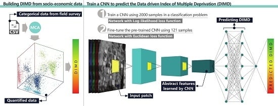
This study aims to map variations of multi-dimensional deprivation among slum settlements providing novel solutions when working in a data-poor environment. “How to meaningfully quantify and aggregate heterogeneous surveyed data into the slums’ degree of deprivation?” is the first research question. To answer this question, this study uses multiple correspondence analysis (MCA) and builds an index based on the Index of Multiple Deprivation (IMD) [34]. We refer to the index as data-driven IMD (DIMD), since the indicators are selected based on the IMD and indicator values are aggregated based on data patterns and MCA. As an advantage over similar studies (e.g., [35]), our method has the potential to be more transferable and less prone to subjectivity. Moreover, collecting data from households is a resource-consuming process which results in limited socio-economic data about slums. This causes a problem for deep learning models as they typically need large datasets to be trained. Therefore, the second question is “How to train a deep CNN to predict slums’ deprivation using VHR satellite images based on limited training samples?” To address this question, a two-step CNN-based approach is performed: I) CNN is trained for a binary classification problem of “slum” and “formal areas” using the log-likelihood loss function. II) The learned spatial features are used to predict the DIMD by fine-tuning the CNN with a small training set using the Euclidean loss function. Unlike other studies (e.g., [19]), we use the CNN for DIMD predictions with a unique framework trained end-to-end. Although this method is not a standard way of training and using a CNN, it can take advantage of the feature learning capability of deep learning models for prediction using very few samples. Few available studies on CNNs and slums (e.g., [29]) use small subsets and use the majority of the area for training to predict the small testing area which is unrealistic for real-world applications.
The following section explains the theoretical framework, available data to this study, and the methods used to analyze the data. Section 3 provides the results and Section 4 discusses the main lessons learned. Section 5 concludes on the utility of CNN-based models to predict the DIMD and suggests possible directions for further studies.
2. Materials and Methods
This study consists of two main steps (Figure 1). First, it analyzes slums based on the concept of deprivation; it characterizes deprivation and processes available socio-economic data from a household survey (HH) and an in-situ quick scan (QS) survey. Second, it builds models based on image features to predict the DIMD. The final result is obtained using an ensemble regression model that combines the result of the CNN with principal component regression (PCR) models based on hand-crafted and GIS features.
The methodology is applied to the Indian city of Bangalore, with a population of more than 10 million and facing rapid slum growth [35,36]. Bangalore is known as the Silicon Valley of India and it is attracting a considerable amount of investment in the ICT sector [37]. However, citizens do not equally benefit from such investments and the growth of wealth has been accompanied by the growth of poverty and consequently the increase of slums [35].
In Bangalore, a wide range of slum settlements exists, from very temporary and worse-off to more permanent and formal-like. All these settlements can be grouped into two administrative categories: notified slums and non-notified slums. Non-notified slums are mostly worse-off, newer settlements, and they are not officially recognized by the government. The government provides basic services to notified slums as well as upgrading programs, which in some cases made them indistinguishable from formal areas [38]. This, together with the availability of remote sensing and reference data, makes it a suitable case for this study.
2.1. Conceptualizing Deprivation
Slums are settlements which are deprived in multiple dimensions, such as poor basic service provision and inadequate housing. To measure the degree of deprivation of such settlements, this study sees deprivation as a multi-dimensional phenomenon [34] covering a wide range of socio-economic and other aspects, which are essential to understanding variations of slum settlements [34]. In the literature, poverty and deprivation have been conceptualized in different ways with a clear shift from one-dimensional approaches looking only at financial aspects, to multi-dimensional approaches [39]. The multi-dimensional poverty index (MPI), introduced by [40], considers health, education, and living standard as three relevant dimensions of poverty. Yet, [41] conceptualized multiple deprivations and defined poverty as the financial aspect of deprivation besides social, environmental, and institutional components. Therefore, regardless of using the term “poverty” or “deprivation”, the importance of looking beyond the financial aspects has been widely emphasized. Aspiring to a broader understanding of deprivation, we adapt the deprivation framework from the IMD developed for Indian cities, which is based on the livelihoods approach [42] and covers four main domains of deprivation; financial, human, social, and physical capitals [34]. This framework focuses on households and the dwelling they live in but does not involve the context of the dwellings. Based on related studies and constructed indices (e.g., [2,10,14,43,44]), the contextual domain was added to the IMD-based deprivation framework to create a holistic picture of deprivation levels. The contextual domain involves indicators, which look at spatial neighborhood characteristics of the geographic area in which the dwelling is located, like accessibility to services or environmental characteristics. One reason that such a comprehensive framework is not used in the related studies is data availability to support the framework (e.g., [32]). Figure 2 shows the five domains of deprivation.
2.2. Available Data
This study uses three main types of data: two sets of socio-economic data, a set of satellite images, and a set of GIS layers. The socio-economic data consists of a set of secondary and a set of primary data. A detailed survey from 1114 households living in 37 notified slums from 2010 (HH data; [45]) is provided by the DynaSlum project [46]. Based on the literature and experts’ knowledge, this study selects 16 indicators (mostly categorical; each indicator contains a number of categories, see Supplementary Materials Section S1 for more details), measuring the five domains of deprivation (Table 1). In addition, the study uses delineated boundaries of 1461 slums from 2017, also provided by DynaSlum. Considering time and resource limitations as well as spatial coverage, primary data about 121 slums were collected. The study calls this primary data collection quick scan (QS) as it is designed in such a way that the surveyor goes to each of the 121 selected slums, observes and documents the surroundings from one location. In this way, the fieldwork covers physical and contextual domains of deprivation for 121 locations, collected within three weeks in August 2017. The dimensions of the QS survey are based on 35 categorical deprivation-related indicators extracted from the literature besides experts’ consultation (Table 1) (see Supplementary Materials Section S2 for more details). The HH and QS data have 26 samples in common (almost 70% of the HH samples) with no significant physical change during the period of 2010 to 2017 (checked on Google Earth). The HH data, which includes indicators from all domains of deprivation, are essential to understand all deprivation components and their variations, while the QS data, which is an up-to-date survey, covers more slum settlements, which is required to build CNN-based models to predict deprivation.
In addition to socio-economic data, the study uses four Pleiades pansharpened satellite images with a spatial resolution of 0.5 m, containing B, G, R, NIR bands, and zero percent cloud coverage, three from March 2016 and one from March 2015, also acquired within the DynaSlum project. Although one of the images was captured on a different date, it helps to have almost a full coverage of the city and is, therefore, used for the analysis. Figure 3 shows the location of slums and the coverage of satellite images.
Furthermore, the study obtains freely available GIS layers using open street map (OSM) data, to extract layers of land use and urban services. These data are not officially validated, though they provide extensive contextual information. Moreover, the study uses world elevation data deriving from multiple sources [47] and having a resolution of 11 m in Bangalore. The elevation data is publicly provided by the ESRI (Environmental Systems Research Institute; [48]).
2.3. Understanding Slums’ Socio-Economic Variations
This study conducts a data-driven approach to analyze deprivation patterns among slums in Bangalore and to understand their variations. Given the categorical nature of the HH and QS data, the study uses MCA, which is a principal component method exclusively developed for categorical data to reduce the number of indicators to a few meaningful dimensions. According to [49], having indicators and categories for a number of individuals, MCA creates a dimensional point cloud and locates individuals in this space based on the scarcity of categories belonging to individuals. The distance of two individuals in the point cloud is defined by the following:
where is the distance between individuals and , is the proportion of individuals having the category ; and are 1 if the category belongs to the individual or and 0 otherwise. Therefore, two individuals with exactly the same categories have the distance of zero and two individuals sharing many categories have a small distance. In other words, individuals with common categories are located around the origin of the point cloud and individuals with rare categories are located at the periphery. Thus, rarer categories are located farther away, and more common categories are gathered closer to the origin. Finally, this high-dimensional space is projected to a low-dimensional space, keeping the most possible variance and the most important variables (which are called dimensions). This study refers to the first dimension created by MCA as the data-driven index of multiple deprivation (DIMD), which delivers a single deprivation value for each individual (i.e., a household in case of the HH DIMD and a slum in case of the QS DIMD). We only use the first dimension created by MCA as it represents indicators with the highest variabilities among individuals. Furthermore, using a single value makes the result of the analysis more comprehensible.
To analyze the socio-economic data, three main steps are followed. First, we use the HH data (a total of 1114 households living in 37 slums) to build the HH DIMD, to identify the deprivation domains which play the most crucial role in differentiating households, and to analyze to what extent households belonging to one slum are homogeneous. Second, we use the QS data (a total of 121 slums) which focus only on physical and contextual domains of deprivation to build the QS DIMD. Third, we explore the correlation between HH and QS DIMDs to find the meaningfulness of relying only on physical and contextual information to analyze the slums’ degree of deprivation in Bangalore. To do this, we use the 26 common samples and compute the Pearson correlation. Samples are bootstrapped 1000 times to derive confidence intervals.
Satellite images are used to predict the QS DIMD solely (and not the HH DIMD) based on two reasons: (1) There are very few HH samples available (i.e., 26 samples), which is an insufficient number to train and validate a CNN, and (2) the available samples were surveyed in 2010, so they are not representative of slums in 2017. Figure 3 shows that HH samples are mostly concentrated in the city center but most of the slums in 2017 are located at the periphery.
2.4. Building Image-Based Models to Predict the DIMD
A deep learning approach is used to analyze satellite images based on a CNN. To train a CNN, one of the most important issues is the “number of samples” [50]. In fact, studies usually use tens of thousands of samples to train CNNs (e.g., [51]). As there are only 121 samples with known DIMD values, we take advantage of 1461 delineated slum boundaries to develop a two-step transfer learning approach. We initially train a CNN with the ability to classify “slums” from “formal areas” using slum boundaries. By training such a network, we learn discriminative spatial features to separate slums from formal residential areas (and consequently, to separate more deprived areas from less deprived areas). Next, we transform the trained network to a regression model by changing its objective function from log-likelihood to Euclidean loss function, which changes the behavior of the network to work as a least square regression model. Based on transfer learning, we use the limited number of samples to fine-tune the new CNN parameters and predict the DIMD. Thus, we use our pre-trained network and its learned features to deal with the few samples available for our study. The process of training CNNs is elaborated in the following sections.
2.4.1. Sample and Image Preparation
We initially train a CNN to classify slums from formal areas. Therefore, 1461 delineated slums are checked one by one on top of the images and slum boundaries are corrected where necessary.
We develop the following strategy to introduce samples of formal areas to the model. A set of 250 × 250 m tessellation is generated on the whole area using stratified random sampling, i.e., dividing the area into squares of 4 × 4 km, and randomly select an equal number of tessellations within each square. This helps to reduce the effect of spatial autocorrelation by generating samples throughout the area, also keeping the samples representative by selecting them randomly within each square [52]. Using OSM, commercial and industrial areas are erased from the delineated formal areas. Thus, 611 polygons are prepared as formal samples. A buffer of 150 m is generated around slum samples and is removed from formal areas to avoid confusion when generating patches on polygons as inputs to the CNN (Figure 4a). This allows us to generate patches up to 200 × 200 pixels (100 × 100 m) on slums and formal areas with no overlap (see orange and red patches illustrated in Figure 4a). Figure 4b shows the final slum and formal samples prepared for this study.
We organize the satellite images for extracting CNN patches. The CNN uses a fixed square patch as input, so one cannot include samples of different sizes as inputs for the same network. However, since slums’ sizes vary significantly, we develop our method in such a way that we can keep all slums of different sizes in our analysis. Based on [10], we generate a 20-m buffer around each sample and change all pixel values outside this buffer to zero for two reasons: (1) Many slums are located between formal areas, so extracted features would not exclusively belong to slums. Consequently, this mixture might bring confusion to the classification accuracy and the predictive model. As an example, the orange patch in Figure 4a is a slum patch but can contain a large number of formal areas depending on where the center point of the patch is located. (2) The same patches can be used to build models based on hand-crafted and GIS features, so the output of the two models are more comparable (Figure 12 shows that some patches have zero values around slums).
Before generating patches from polygons (Figure 4), we randomly select two-third of our polygon samples for training/validation and one third for testing. Therefore, these two sets are completely independent. Furthermore, for training and validation, we generate two independent point sets as path centers, then extract patches accordingly.
2.4.2. CNN-Based Model to Predict the DIMD
Classification Problem
Figure 5 shows the steps taken to do the classification task. A detailed explanation of each step follows.
To generate patches as input to the CNN, we first generate patch center points on the sample polygons, then extract each patch accordingly. A shallow CNN is trained using 1000 training and 1000 validation patches with patch sizes of 99, 129, and 165 pixels to find the optimal patch size. The shallow network [23] contains two convolutional layers followed by a fully-connected layer and a softmax classifier with a log-likelihood objective function (Figure 6).
In each convolutional layer, a 2D convolution is performed with shared weights and biases within a kernel as follows:
where is the shared bias, is a array with shared weights, denotes the activation position within a kernel with the origin of , and is the rectified linear unit (ReLU) activation function. The process is followed by a max pooling layer with the size of .
Extracted features feed a one-dimensional fully-connected layer followed by a softmax classifier. Using the softmax classifier, in addition to the classification result, the network returns the probability of each patch belonging to each class as follow:
where is the probability of class , is the activation value of the corresponding output class, and the denominator is the sum of the probability of all classes (). The network is trained by using log-likelihood loss function as follows:
where is the number of samples, is the total number of classes, is the true vector, and is the predicted vector by the network. Network parameters are optimized using the stochastic gradient decent method and the backpropagation algorithm [53].
To regularize the network, we use drop-out layers with a rate of 0.5 after each pooling layer [54]. We keep the drop-out rate of 0.5 throughout the analysis as our deep network is inspired by VGG [51], which uses this rate in [55]. We initialize weights as sqrt(2/number of input neurons) based on [56] to prevent saturation in the network and to increase learning pace. Moreover, we give higher learning rates for the first epochs and gradually decrease it when the learning curve is converging to speed-up the learning process. The network is allowed to train to a maximum of 700 epochs to make sure that the loss function is minimized. We prevent overfitting by using drop-out and stochastic gradient descent with mini batches. We also monitored both training and validation loss functions after each epoch to make sure they have a similar decreasing pattern. Figure 6 shows the architecture of the shallow CNN and Table 2 shows a summary of the network’s hyper-parameters. Training the network is carried out with MATLAB and MatConvNet library [57]. We compiled networks on the GPU which significantly improves the learning speed [57]. This study trains networks on an NVIDIA QUADRO 1000M GPU with CUDA toolkit and cuDNN library.
We also take advantage of using popular networks in the field of image recognition to train a deeper CNN. Since these networks only accept patches with three channels as input and our images have four channels, we train a network from scratch inspired by visual geometry group (VGG-F) [51] to solve our classification problem. The network is deep enough to solve the ImageNet large-scale visual recognition challenge (ILSVRC), but it is computationally not too expensive, so we can train it on a GPU with 2GB of RAM having inputs of four channels. The original VGG networks use local response normalization (LRN) [51], but we use batch normalization (BNorm) instead, since it is more effective [58] (Figure 7). Both shallow and deep CNNs are trained using 2000 training and 2000 validation patches to compare the performance of the two networks.
Using image augmentation, we increase the number of training patches [59]. Based on [26], each patch is rotated in seven directions; 7, 90, 97, 180, 187, 270, and 277 degrees with linear interpolation. Therefore, the deep network is trained again using 16,000 training patches to explore any improvement by using image augmentation. The accuracy of the best-performing network is assessed using 2000 independent test patches.
Transfer Learning: Regression Problem
We use the best-performing network to solve the regression problem and predict the DIMD by transfer learning. The loss function is changed to Euclidean loss as follow:
As there are only 121 samples to fine-tune the network, we use 10-fold cross-validation to assess the performance. To evaluate the overall predicting power of the model, we calculate the coefficient of determination (R2) on the validation samples. We use R2 to evaluate our models as it is a common way to assess a model’s performance in this field (e.g., [19,31,32]), and the measure is unitless so this makes the results more comparable across study areas and with results of similar studies.
2.4.3. PCR Models Using Hand-Crafted and GIS Features
This study employs principal component regression (PCR) models using hand-crafted image features and GIS features extracted from the slum patches to (1) compare the result of building models based on these features with CNN results, and, (2) explore possible improvements these features can bring to the CNN results. Training PCR models enables the use of many features, reducing them to a few components, and building regression models with components to predict the DIMD. Table 3 lists the extracted features, covering three groups:
- Spectral information (Table 3; Spectral info.).
- Two sets of the most common texture features; grey level co-occurrence matrix (GLCM) and local binary pattern (LBP). We generate GLCM features in four directions and four lags (i.e., 1 to 4 pixels) and based on [17], we calculate three properties—entropy, variance, and contrast—on each feature. We calculate GLCM properties on each band of a patch and consider the mean value as the property value (Table 3; GLCM).
- To include LBP features in the model, we extract only uniform patterns (with a maximum of two transitions), which provide the most important textural information about an image [60]. Based on [18], we calculate (i.e., rotation invariant uniform patterns with a radius of 1, which considers eight neighbors), , and with linear interpolation. We average the extracted LBP of each band to obtain the value for a patch considering the whole patch as a cell (Table 3; LBP).
- GIS features; as road data are not consistent enough to perform network analysis, we calculate the minimum Euclidean distances from each of the public service/land use (Table 3; GIS) to a patch’s center points. Distance to different land uses and public services have been used to calculate the degree of deprivation of settlements especially in UK deprivation indices (e.g., [44]). We consider the town hall as the center of the city, which is very close to the geographic center of the city. Using the elevation layer, we calculate the mean elevation and mean slope within each patch.
We use the extracted features to feed stepwise PCR models. Different combinations of features are trained, with a different number of components, and different model complexities (pure linear; linear allowing interaction, i.e., multiplication of two components as a new variable; and quadratic allowing interaction) (Figure 8). For the evaluation, 10-fold cross-validation is used.
2.4.4. Ensemble Regression Models
We build ensemble regression models using the outputs of the best performing CNN and PCR models. These ensemble models are trained, varying the complexity from linear to polynomial.
3. Results
3.1. DIMDs
Figure 9a shows the squared correlation R2 between HH indicators and the HH DIMD. It shows that electricity, floor material, wall material, toilet, roof material, and water sources have the largest contribution to build the HH DIMD and to explain variations across the 1114 households.
Interpreting households along the HH DIMD gives an overview of the variations of households within a slum and confirms the meaningfulness of aggregating DIMD values for a slum settlement. Figure 9b plots the aggregated HH DIMD value of households within each slum by calculating the mean and standard deviation. Slums with a value around the origin (i.e., zero) have the most common (or average) pattern of categories and slums with high and low values are clearly distinct. Considering the slums along the HH DIMD and comparing the values with the ground situation and HH data, we find that negative HH DIMD values represent worse-off slums and positive HH DIMD values represent better-off slums in terms of deprivation. Regarding the range of values, worse-off slums are significantly different from the common pattern, but it is not the case for better-off slums. Figure 9b also shows that the internal variation in the better-off slums is less than in the worse-off slums. Although these variations are quite high in some cases, considering standard deviations, it is meaningful to measure one single value as the DIMD for each slum because households living in one slum have mostly close DIMD values, meaning they have a similar situation in terms of basic services like electricity, and construction material of the dwellings (Figure 9a).
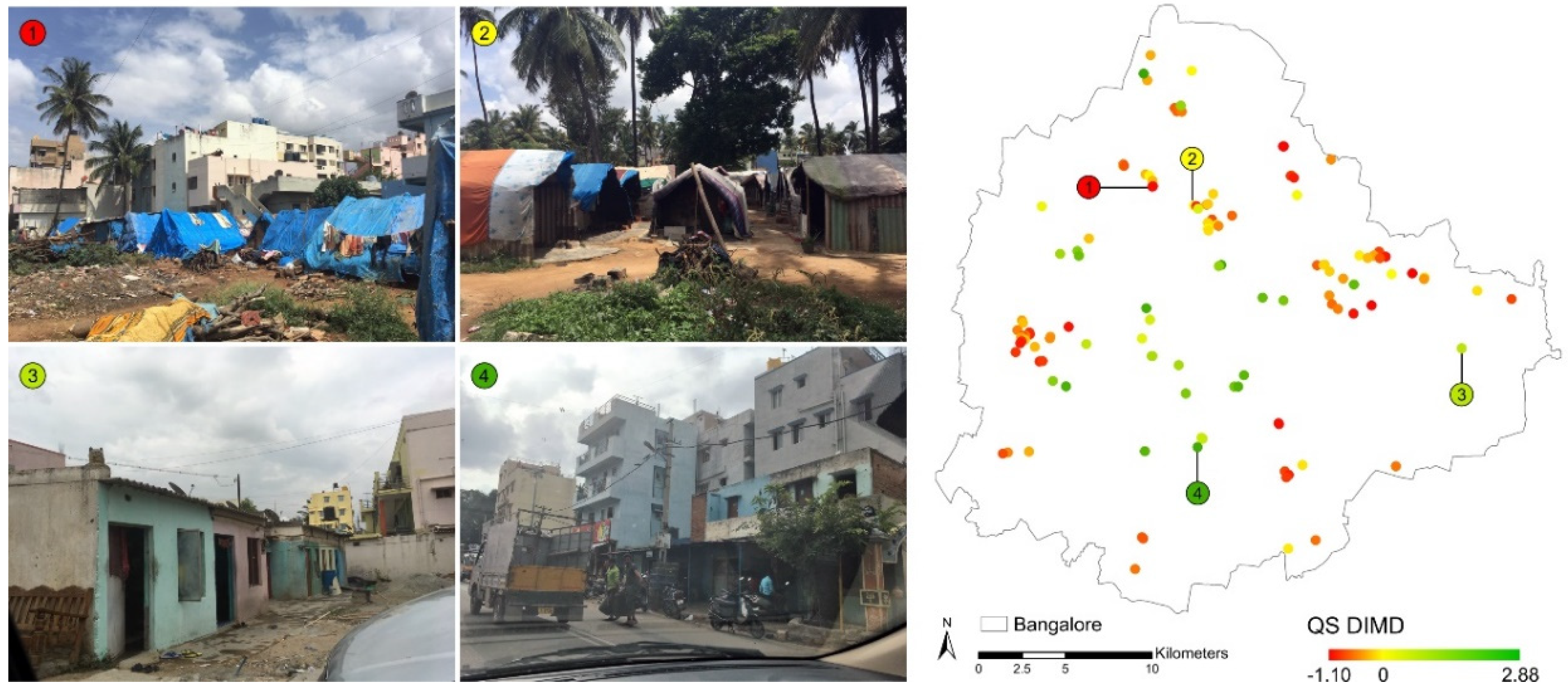
By performing MCA on the QS samples, which are more diverse and have larger spatial coverage than the HH samples, we create a more comprehensive pattern of deprivation of slums. Figure 10 shows the QS samples with their QS DIMD values on a map. It also shows four sample photos (taken during the QS fieldwork) having the smallest to largest DIMD values. Considering the value range of the DIMD, better-off slums are significantly different from the common pattern, but the worse-off slums are less different (see Figure 10 sample number 2 with a value around zero and compare it to the high-end and the low-end values). This is also shown by the photos displaying the ground situation.
The result of exploring the relationship between the two DIMDs shows a significant correlation coefficient R of 0.63 (p = 0.0006) with positive confidence intervals [0.28, 0.82] (95% confidence intervals). This means we are 95% confident that the two DIMDs are positively correlated among the whole slums in Bangalore with a coefficient in the range of [0.28, 0.82]. In this sense, the two DIMDs are both describing deprivation (as they are correlated) and it is meaningful to use the QS DIMD as a measure of deprivation. However, they look at the deprivation concept from different perspectives. This means one cannot fully explain variations of the other. This is indicated by a R2 is 0.40 [0.08, 0.67]. We should also consider the temporal gap between the HH and QS data. Although the 26 samples are checked using Google Earth to ensure they have not significantly changed since 2010, there is a possibility that some of them experienced changes which are not visible in satellite images.
3.2. CNN-Based Model Performance
The result of training shallow to deep CNNs are shown in Figure 11. Figure 11a shows the result of the shallow CNNs with different patch sizes. The patch size of 129 results in the highest accuracy on the validation set, and, thus, we use this patch size to train shallow and deep CNNs again with 2000 training/validation samples. Figure 11b shows the obtained accuracy using the shallow network with 2000 training samples, the deep network with 2000 training samples, and the deep network with image augmentation and 16,000 training samples. Comparing the performance of the shallow network with the deep one using the same number of samples, the classification error drops by almost 50% (from 7.00% to 3.50%). This shows the advantage of using deeper networks and extracting more abstract features. Taking advantage of image augmentation, the classification error drops by almost 40% (from 3.50% to 1.44%), and we reach the overall accuracy of 98.56% on the validation set.
Using the 2000 test patches on the best-performing CNN, we reach the accuracy of 98.40%. Figure 12 shows some slum patches (test set) classified by this network. All these patches are slums, but some are incorrectly classified as formal. The percentages below the patches show the confidence of the network in classifying these patches as slums (derived from the softmax layer). Scores of less than 50% result in classifying patches as formal. Patches like number 1 are clearly classified as slums. They have very distinct characteristics with small dwellings and irregular patterns, easily distinguishable from formal areas. Slums like number 2 with some regular patterns are classified as slums with less confidence. Patch 3 is challenging, containing small slums between formal areas. Although it is not easy to identify the slum area between formal areas, it is also correctly classified. Patch 4 and 5 have almost the same situation but dwellings in patch 5 are tiny and we cannot even confidently recognize them by sight. Patches like number 6 completely confuse the network as they have larger dwellings with some regular patterns. Overall, only 1.92% of slum patches (19 out of 1000 patches) are classified incorrectly (Figure 12).
We fine-tune the pre-trained CNN with its learned distinctive features to directly predict the QS DIMD values and train each network for 100 epochs to ensure convergence. The model predicts the QS DIMD with the R2 of 0.67.
3.3. PCR Model Performance
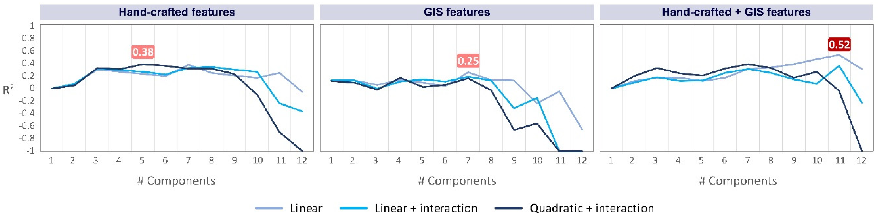
As a supplementary step, we train PCR models based on manually extracted hand-crafted and GIS features. We develop three categories of models; using only hand-crafted features, using only GIS features, and using both hand-crafted and GIS features (Figure 13).
Using only hand-crafted features, the R2 of 0.38 is obtained. Relying only on GIS features, the model can reach the R2 of 0.25. The best model is trained using both hand-crafted and GIS features, involving 11 components in a linear regression that delivers the R2 of 0.52. The R2 values below −1 are plotted as −1 for better visualization.
3.4. Ensemble Models
We build ensemble models with different complexities in three combinations; CNN + hand-crafted + GIS, CNN + hand-crafted, CNN + GIS (Table 4). The best result is obtained using the combination of all the three categories of features in a 3rd degree polynomial regression with the R2 of 0.75.
To explore our final ensemble model (with R2 of 0.75), we visualized a scatter plot of QS DIMD and predicted values in Figure 14, as well as the six worst-off and the six best-off slums predicted by the model in Figure 15. The model has the RMSE value of 0.53 and the BIAS of 0.20. BIAS is calculated by averaging the BIAS of all predictions and shows, on average, that the model tends to predict values 0.2 units higher than the observed value. RMSE shows that the average error in each prediction is 0.53 units. When variation at the negative side of the QS DIMD is less, the model performs better. This can be confirmed by comparing QS DIMD and predicted values. On the positive side, although the DIMD is mostly predicted well, there is still some confusion in the model (see best-off slums number 2 and 3 in Figure 15). Comparing number 2 and 4 of the best-off slums in Figure 15, patches are very similar, and indicators that make number 2 worse than number 4 in the DIMD might not be visible in remote sensing images. It can also be an error coming from the fieldwork as in the QS fieldwork the surveyor was standing on one point and reported what was visible. There is a possibility that this point is different from the typical structure of that slum, especially in large settlements. The other source of error can be using a fixed square patch to extract features from all the slums. Some settlements are large, and a patch can cover a small area of them; however, some settlements are tiny, and even if we consider their context (i.e., 20-m buffer), a patch is bigger than the area of the analysis. Thus, we ignore all the area of the large settlements except a patch located at the center and there is a possibility that the patch does not represent the whole area of the settlement.
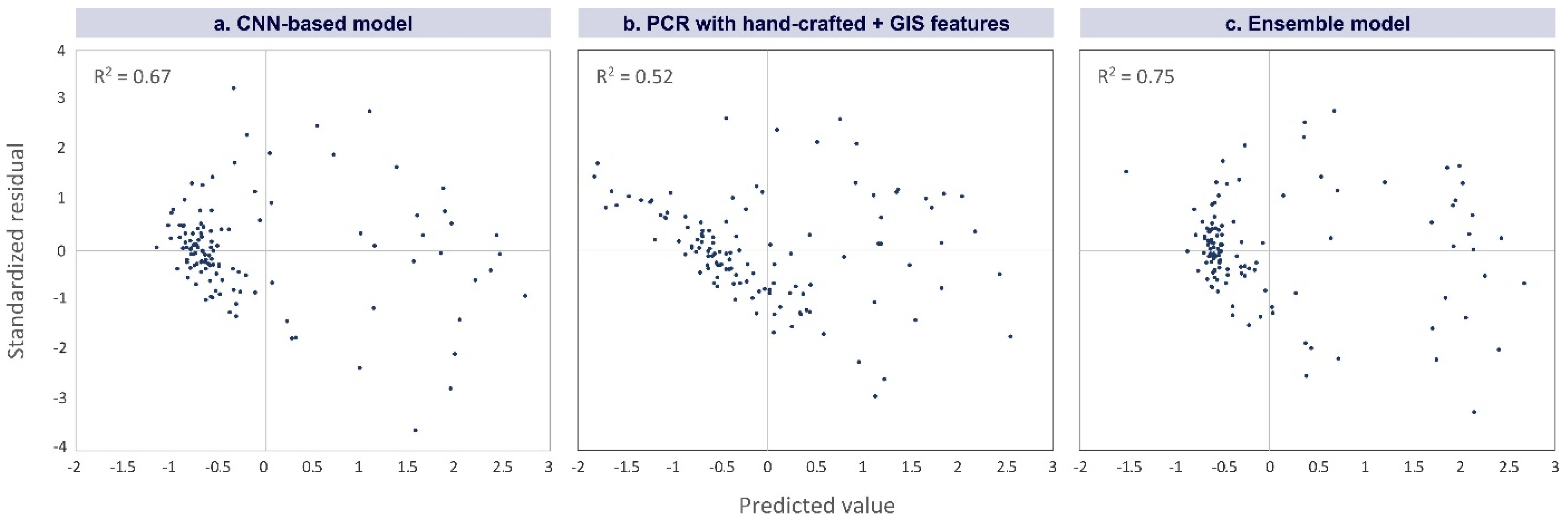
To have a more in-depth look at the performance of the models and assess their generalization capability, prediction errors are plotted and explored. We focus on the model created by the CNN with R2 of 0.67, the model created with hand-crafted and GIS features with R2 of 0.52, and the ensemble model created by combining CNN, handcrafted, and GIS results with R2 of 0.75. One crucial assumption to consider when one wants to generalize a model is homoscedasticity, i.e., expecting the same variance of residuals across the whole range of predicted values [61]. Figure 16 plots standardized residuals over predicted values of the three models. Optimally, there should be scattered points without any systematic pattern; however, our plots violate this assumption and we can find different patterns among negative and positive predicted values. The errors are less evenly distributed on the negative side of the models based on CNN (Figure 16a), and hand-crafted + GIS features (Figure 16b). Nevertheless, in all plots, residuals have different patterns on the negative and positive sides. Comparing Figure 16 and Figure 10, less difference (more homogeneity) results in less variance in the residuals. The worse-off slums are more similar to each other, so the predictions also have smaller errors. However, better-off slums are very different from each other. Comparing photo 2 and 4 in Figure 10, there is a wide difference between the average situation (i.e., value 0) and the best-off slum. Therefore, residuals have more variance, and the predictions are less accurate. For instance, consider photo 2 and 3 of the best-off slums in Figure 15, the model has larger errors.
4. Discussion
This study proposes data-driven methods for creating a deprivation index as a solution to the classical deprivation indices, many of which suffer from subjective weights assignment, as well as predicting the index from VHR satellite images using CNN. The aim is to build a comprehensive understanding of socioeconomic variations of slums, covering multiple domains of deprivation, and provide information for designing targeted policies to support, upgrade, and monitor such settlements. We show the ability of VHR satellite images to predict the degree of deprivation even for tiny slums with few dwellings. Our method can capture deprivation of any type of slum in Bangalore regardless of its size. The proposed method enables dealing with the small number of available training samples to train a CNN for predicting the DIMD by a two-step transfer learning process that is a clear innovation compared to other studies using a small subset and taking most of the areas of training to predict a small part that was used. This helps to take advantage of deeply learned features in solving problems related to slum studies which always suffer from limitations of data availability. Most studies focus on distinguishing slums from formal settlements as a binary classification and do not offer the possibility to estimate a continuous index to characterize the deprivation level using CNNs (e.g., [29,31]).
We use the MCA method to build deprivation indices by a data-driven approach with few assumptions. Categorical indicators are used without manipulation, and index values are assigned to individuals based on the patterns of categories. We find that relying only on the pattern of data, without pre-assumptions like ordering categories and assigning pre-defined weights, it is possible to distinguish the better-off, the worse-off, and the average situation of slum settlements with their relative differences. For instance, [35] ordered categorical data, transferred them to ordinal data, and aggregated them using descriptive statistics to build a slums index. Similarly, [43] aggregated indicators of a deprivation index with equal weights. Although these methods are very common and based on experts’ knowledge, they might include many assumptions and bias the result. Based on our data-driven approach, the importance of deprivation dimensions is not the same. Comparing the DIMD values with the ground situation, we can empirically prove that the first dimension of deprivation provides a meaningful measure, showing the variability of deprived areas across a quantitative range (see Supplementary Materials Section S3 for ground photos of slums with respective QS DIMD values).
We show that the indicators related to the physical capital play the most crucial role in distinguishing slum types. These two domains also shape the visible features from the satellite image. Therefore, the method is based on the assumption that these two domains contribute to building the DIMD.
There are also some limitations to using MCA. Our approach is meaningful when there is a set of representative samples available. Non-representative samples, like the HH samples, which are not a good representation of slums in 2017, result in less meaningful DIMD values. Considering Figure 9b and Figure 10, and comparing the range of the two DIMDs, almost opposite trends of skewness are shown. The average situation of the HH DIMD is more similar to the better-off slums, but in the case of the QS DIMD, the better off slums are significantly different from the average situation. This shows that the HH samples are mostly covering the better-off and are not a sufficient representation of all slums in Bangalore in 2017. In fact, the HH samples cover only the notified slums and they have often received upgrading from the government, but QS samples also include non-notified slums which are not included in official slum data in India. It is also important that the data contains only deprivation-related indicators. If non-related indicators are included and they contain information which is highly different across slums, it will bias the result significantly. Other less data-dependent options to create an index can be used in the case of non-representative or not well-distributed samples, which consider experts’ knowledge, for example, by means of analytic hierarchy process (AHP) [62].
Using all hand-crafted + GIS features, 11 components, and a linear PCR model, we obtain R2 of 0.52 to predict the DIMD. Comparing this result with the CNN result, the CNN with R2 of 0.67 outperforms our complex PCR models. For a better comparison, we should compare the CNN result with the result of the regression using only hand-crafted features as the CNN also does not consider where the patches are located. In this manner, we have the R2 of 0.38 from hand-crafted features using a quadratic model in comparison with R2 of 0.67 from the CNN. This shows the advantage of using deeply learned features by the CNN over hand-crafted features and the PCR model. More sophisticated hand-crafted features as extracted in many studies like [10] and [20] might improve the result. The features we use to train the PCR models can be generated for any study area, but the importance of the features might be different. For the transferability of the method, future studies can focus on the overall methodology, instead of single features. We show that by adding GIS layers to hand-crafted features, the result can be boosted significantly. Besides regression models with different complexities, it is worth exploring the ability of other machine learning methods to predict the DIMD. For example, [19] showed GBR and RF could outperform a linear regression model, so it is worth exploring such algorithms in further studies. Furthermore, future studies can train CNNs optimizing more parameters (and hyper parameters). For instance, we used drop-out layers with a rate of 0.5, but it is worth exploring lower values as well.
Using the combination of hand-crafted + CNN, the R2 remains 0.67. This means the hand-crafted features cannot contribute to improving CNN extracted features. However, the result from the GIS layers can improve the CNN result to 0.71. This means by adding the GIS layers, we include additional information to the CNN. The best result obtained is 0.75 by using CNN + hand-crafted + GIS in a third-degree polynomial model, allowing interaction between variables. This shows that, although hand-crafted features cannot improve the result of the CNN, their interactions with GIS features can bring improvements to the model. We conclude that using GIS layers in parallel with CNN can bring improvements to the model as basically a CNN does not consider the spatial location of patches. We also show that the CNN-based model has more capabilities of generalization compared to the PCR model as the error values are more normally distributed. Although the BIAS value in the best-performed model is low (0.20), the RMSE value (0.53) shows that there is a risk to consider worse-off slums as more common settlements as the value range of the worse-off slums is very low (i.e., between −1.10 and 0). This shows a potential to overestimate the model performance if we only consider the R2 value, especially for samples in the negative side.
Figure 16 shows that slums having positive DIMD values have distinct error patterns compared to the negative side. This proves the fact that slums are forming groups/types which are very different from each other. Furthermore, it shows that the label slum covers very diverse areas. In the case of Bangalore, our analysis shows two main different groups of slums, but research on other cities might find more groups of slums, leading to a more diverse typology.
Spatial independence of samples is a crucial assumption in regression models and it also affects the result of accuracy assessment. By looking at Figure 10 (QS samples) we can see spatial clusters of slums which represents the spatial dependency of the samples. The problem comes from two sources. First, slums are not evenly distributed across the city (which is very common across cities with slum areas). Second, to maximize the number of collected samples within the time available, we collected samples from selected clusters. To deal with the problem of autocorrection, we sampled dispersed clusters and selected random samples within clusters. To create folds, we selected slums randomly from all clusters. We also created each CNN patch from a different slum sample to make sure there is no overlap, which means that patches are not created from the same slum (to avoid violating the requirement of independence). Therefore, our folds are less spatially correlated. Furthermore, we added the GIS layers that provide insights into the spatial organization of the samples. In fact, we used GIS layers as spatial components to the model. Further studies might bring spatial components to the model using other methods like Lagrange Multiplier [7].
Relying on data-driven approaches, the method is transferable to other contexts. Both MCA and CNN analyze data with no need for data manipulation, so it is possible to feed them with new samples. Relying on hand-crafted features, developed methods are always context-specific and are rarely transferable to another context (e.g., [10,31,63]). However, CNN automatically extracts features based on training samples, so it determines the most important features itself. It is needed to tune CNN hyperparameters and patch size, but the overall approach remains the same. It is also possible to measure deprivation/socio-economic characteristics (in the case of available socio-economic data) of areas other than slums with the same approach. In some contexts, there are areas which are deprived but not labeled slums administratively [34]. Thus, it is relevant to apply this method to a whole range of existing settlements in a specific context and explore their relative differences.
5. Conclusions
This study analyzed the relationship between slum variations from the perspective of deprivation with image-based features. The use of two main data-driven approaches (i.e., MCA and CNN) to analyze socio-economic data and VHR satellite images distinguishes this research from related previous studies. The combination of the two methods built a holistic methodological framework that could use surveyed data and satellite images as inputs and perform analyses with no need for data manipulation. This, coupled with our two-step transfer learning approach to train a deep CNN dealing with a limited number of training samples, resulted in an R2 of 0.75 to predict slums’ degree of deprivation in Bangalore using VHR imagery. The high diversity of slum settlements makes it challenging to build a single unbiased model to predict the degree of deprivation. Although the model showed different behavior in predicting better-off and worse-off slums, the proposed method opens the door to explore the possibility of building models with a better generalization capability. To deal with the issue of heteroscedasticity, two possible solutions can be followed by further studies: First, using common statistical methods like value transformation (e.g., log transformation) of the DIMD values, or switching to weighted least square regression from ordinary least square which could be integrated into the CNN and PCR models; second, dividing slums into two worse-off and better-off groups (i.e., slums with a negative DIMD value and slums with a positive DIMD value), so it is more likely to create models with less biased predictions. However, this solution needs more samples, especially with positive DIMD values. The study simplified slum samples by creating a 20m buffer and changing the pixel values outside the buffer to zero. Although we added this step to prevent confusion to the CNN models, further studies can train CNN models that can deal with this without this pre-processing step. This study combined GIS layers with the CNN in an ensemble model; however, the possibility of integrating GIS layers within the CNN framework is worth exploring. One option to explore in further studies is to create GIS features and add them to the original patches as new image channels. Suppose instead of having only a 4-channel image, we add new GIS-based channels as inputs to the CNN and let it solve the regression problem. Indeed, this needs high computational capacity as adding new channels increases the number of CNN parameters significantly. Furthermore, the transferability to other contexts or focusing on other types of settlements other than slums need further exploration. In respect to the creation of DIMD, we used the first dimension created by MCA to analyze deprivation along two sides (i.e., positive and negative). Further studies can add the second dimension, analyzing individuals in a two-dimensional space along four sides, and predict both dimensions using transfer learning. Ultimately, the developed model enables a deeper understanding of slums in Bangalore and can help policymakers to prioritize and establish pro-poor people-based policies to address people’s needs. It characterizes spatial patterns of deprivation relying on satellite images and helps to understand where the deprivation is, and what should be the target of upgrading programs to address it. Furthermore, the output of this model can be used to feed other models like agent-based models to simulate and predict the dynamics of such settlements. It is a possibility to connect the result of this work to studies related to health, well-being, and urban land-use modeling to create a basis and help policymakers establish effective policies towards enhancing the quality of life.
Supplementary Materials
The following are available online at https://www.mdpi.com/2072-4292/11/11/1282/s1, Section S1: HH data; Section S2: QS data; Section S3: Ground photos from QS samples.
Author Contributions
A.A. performed the data analyses and wrote the majority of the paper. M.K., C.P., and K.P. supported in developing the structure of the paper, supervision, and revising the paper.
Funding
We would like to acknowledge the support of the SimCity project (contract number: C.2324.0293) for data collection and the support from the NWO/Netherlands eScience Center funded project DynaSlum—Data Driven Modelling and Decision Support for Slums—under the contract number 27015G05.
Acknowledgments
We would like to express our great appreciation to Chloe Pottinger-Glass who carried out the fieldwork and collected the data used to build the QS index; this also includes the photographs used in this article. We would like to acknowledge the support of the SimCity project (contract number: C.2324.0293) and the support from the NWO/Netherlands eScience Center funded project DynaSlum—Data Driven Modelling and Decision Support for Slums—under the contract number 27015G05. We wish to offer our special thanks to Champaka Rajagopal for their help in providing a deeper local insight into the available data and setting up the QS fieldwork. We are particularly grateful to Debraj Roy and Mike Lees from the University of Amsterdam (DynaSlum project leaders) and Berend Weel from eScience Center for granting access to the data acquired within DynaSlum.
Conflicts of Interest
The authors declare no conflict of interest.
References
- United Nations. World Urbanization Prospects, The 2014 Revision; United Nation: New York, NY, USA, 2014. [Google Scholar]
- Kohli, D.; Sliuzas, R.; Kerle, N.; Stein, A. An ontology of slums for image-based classification. Comput. Environ. Urban Syst. 2012, 36, 154–163. [Google Scholar] [CrossRef]
- Mahabir, R.; Croitoru, A.; Crooks, A.; Agouris, P.; Stefanidis, A.; Mahabir, R.; Croitoru, A.; Crooks, A.T.; Agouris, P.; Stefanidis, A. A Critical Review of High and Very High-Resolution Remote Sensing Approaches for Detecting and Mapping Slums: Trends, Challenges and Emerging Opportunities. Urban Sci. 2018, 2, 8. [Google Scholar] [CrossRef]
- UN-Habitat. Informal Settlements; UN-Habitat: New York, NY, USA, 2015. [Google Scholar]
- UN-Habitat. The Challenge of Slums—Global Report on Human Settlements; Earthscan Publications Ltd.: London, UK, 2003. [Google Scholar]
- Arimah, B.C. The Face of Urban Poverty: Explaining the Prevalence of Slums in Developing Countries. In Urbanization and Development; Oxford University Press: Oxford, UK, 2010; pp. 143–164. [Google Scholar] [Green Version]
- Duque, J.C.; Patino, J.E.; Ruiz, L.A.; Pardo-Pascual, J.E. Measuring intra-urban poverty using land cover and texture metrics derived from remote sensing data. Landsc. Urban Plan. 2015, 135, 11–21. [Google Scholar] [CrossRef]
- Nijman, J. Against the odds: Slum rehabilitation in neoliberal Mumbai. Cities 2008, 25, 73–85. [Google Scholar] [CrossRef]
- Patel, S.; Baptist, C. Editorial: Documenting by the undocumented. Environ. Urban. 2012, 24, 3–12. [Google Scholar] [CrossRef]
- Kuffer, M.; Pfeffer, K.; Sliuzas, R.; Baud, I.; Maarseveen, M. Capturing the Diversity of Deprived Areas with Image-Based Features: The Case of Mumbai. Remote Sens. 2017, 9, 384. [Google Scholar] [CrossRef]
- Duque, J.C.; Royuela, V.; Noreña, M. A Stepwise Procedure to Determinate a Suitable Scale for the Spatial Delimitation of Urban Slums. In Defining the Spatial Scale in Modern Regional Analysis; Fernández Vázquez, E., Rubiera Morollón, F., Eds.; Springer: Berlin/Heidelberg, Germany, 2013; pp. 237–254. ISBN 978-3-642-31994-5. [Google Scholar]
- Olthuis, K.; Benni, J.; Eichwede, K.; Zevenbergen, C. Slum Upgrading: Assessing the importance of location and a plea for a spatial approach. Habitat Int. 2015, 50, 270–288. [Google Scholar] [CrossRef]
- Munyati, C.; Motholo, G.L. Inferring urban household socio-economic conditions in Mafikeng, South Africa, using high spatial resolution satellite imagery. Urban Plan. Transp. Res. 2014, 2, 57–71. [Google Scholar] [CrossRef]
- Thomson, C.N.; Hardin, P. Remote sensing/GIS integration to identify potential low-income housing sites. Cities 2000, 17, 97–109. [Google Scholar] [CrossRef]
- Weeks, J.R.; Hill, A.; Stow, D.; Getis, A.; Fugate, D. Can we spot a neighborhood from the air? Defining neighborhood structure in Accra, Ghana. GeoJournal 2007, 69, 9–22. [Google Scholar] [CrossRef] [Green Version]
- Williams, N.; Quincey, D.; Stillwell, J. Automatic Classification of Roof Objects from Aerial Imagery of Informal Settlements in Johannesburg. Appl. Spat. Anal. Policy 2016, 9, 269–281. [Google Scholar] [CrossRef]
- Kuffer, M.; Pfeffer, K.; Sliuzas, R.; Baud, I. Extraction of Slum Areas from VHR Imagery Using GLCM Variance. IEEE J. Sel. Top. Appl. Earth Obs. Remote Sens. 2016, 9, 1830–1840. [Google Scholar] [CrossRef]
- Ella, L.P.A.; van den Bergh, F.; van Wyk, B.J.; van Wyk, M.A. A Comparison of Texture Feature Algorithms for Urban Settlement Classification. In Proceedings of the IGARSS 2008—2008 IEEE International Geoscience and Remote Sensing Symposium, Boston, MA, USA, 7–11 July 2008; Volume 1, pp. III-1308–III-1311. [Google Scholar]
- Arribas-Bel, D.; Patino, J.E.; Duque, J.C. Remote sensing-based measurement of Living Environment Deprivation: Improving classical approaches with machine learning. PLoS ONE 2017, 12, 1–25. [Google Scholar] [CrossRef] [PubMed]
- Duque, J.C.; Patino, J.E.; Betancourt, A. Exploring the potential of machine learning for automatic slum identification from VHR imagery. Remote Sens. 2017, 9, 895. [Google Scholar] [CrossRef]
- Schug, F.; Okujeni, A.; Hauer, J.; Hostert, P.; Nielsen, J.Ø.; van der Linden, S. Mapping patterns of urban development in Ouagadougou, Burkina Faso, using machine learning regression modeling with bi-seasonal Landsat time series. Remote Sens. Environ. 2018, 210, 217–228. [Google Scholar] [CrossRef]
- Taubenböck, H.; Kraff, N.J.; Wurm, M. The morphology of the Arrival City—A global categorization based on literature surveys and remotely sensed data. Appl. Geogr. 2018, 92, 150–167. [Google Scholar] [CrossRef]
- Bergado, J.R.A.; Persello, C.; Gevaert, C. A Deep Learning Approach to the Classification of Sub-Decimetre Resolution Aerial Images. In Proceedings of the 2016 IEEE International Geoscience and Remote Sensing Symposium (IGARSS), Beijing, China, 10–15 July 2016; pp. 1516–1519. [Google Scholar]
- Bergado, J.R.; Persello, C.; Stein, A. Recurrent Multiresolution Convolutional Networks for VHR Image Classification. IEEE Trans. Geosci. Remote Sens. 2018, 56, 6361–6374. [Google Scholar] [CrossRef] [Green Version]
- Castelluccio, M.; Poggi, G.; Sansone, C.; Verdoliva, L. Training convolutional neural networks for semantic classification of remote sensing imagery. In Proceedings of the 2017 Joint Urban Remote Sensing Event, Dubai, UAE, 6–8 March 2017; pp. 1–4. [Google Scholar] [CrossRef]
- Scott, G.J.; England, M.R.; Starms, W.A.; Marcum, R.A.; Davis, C.H. Training Deep Convolutional Neural Networks for Land-Cover Classification of High-Resolution Imagery. IEEE Geosci. Remote Sens. Lett. 2017, 14, 549–553. [Google Scholar] [CrossRef]
- Huang, B.; Zhao, B.; Song, Y. Urban land-use mapping using a deep convolutional neural network with high spatial resolution multispectral remote sensing imagery. Remote Sens. Environ. 2018, 214, 73–86. [Google Scholar] [CrossRef]
- Zhang, C.; Sargent, I.; Pan, X.; Li, H.; Gardiner, A.; Hare, J.; Atkinson, P.M. An object-based convolutional neural network (OCNN) for urban land use classification. Remote Sens. Environ. 2018, 216, 57–70. [Google Scholar] [CrossRef] [Green Version]
- Mboga, N.; Persello, C.; Bergado, J.R.; Stein, A. Detection of informal settlements from VHR satellite images using convolutional neural networks. In Proceedings of the 2017 IEEE International Geoscience and Remote Sensing Symposium (IGARSS), Fort Worth, TX, USA, 23–28 July 2017; Volume 7, pp. 5169–5172. [Google Scholar]
- Persello, C.; Stein, A. Deep Fully Convolutional Networks for the Detection of Informal Settlements in VHR Images. IEEE Geosci. Remote Sens. Lett. 2017, 14, 2325–2329. [Google Scholar] [CrossRef] [Green Version]
- Engstrom, R.; Newhouse, D.; Haldavanekar, V.; Copenhaver, A.; Hersh, J. Evaluating the relationship between spatial and spectral features derived from high spatial resolution satellite data and urban poverty in Colombo, Sri Lanka. In Proceedings of the 2017 Joint Urban Remote Sensing Event (JURSE), Dubai, UAE, 6–8 March 2017; pp. 1–4. [Google Scholar]
- Jean, N.; Burke, M.; Xie, M.; Davis, W.M.; Lobell, D.B.; Ermon, S. Combining satellite imagery and machine learning to predict poverty. Science 2016, 353, 790–794. [Google Scholar] [CrossRef] [Green Version]
- Ministry of Housing Communities & Local Government English. Indices of Deprivation. Available online: https://www.gov.uk/government/statistics/english-indices-of-deprivation-2015 (accessed on 11 August 2017).
- Baud, I.; Sridharan, N.; Pfeffer, K. Mapping Urban Poverty for Local Governance in an Indian Mega-City: The Case of Delhi. Urban Stud. 2008, 45, 1385–1412. [Google Scholar] [CrossRef]
- Rains, E.; Krishna, A.; Wibbels, E. Combining satellite and survey data to study Indian slums: Evidence on the range of conditions and implications for urban policy. Environ. Urban 2018, 31, 267–292. [Google Scholar] [CrossRef]
- United Nations. The World’s Cities in 2016: Data Booklet; United Nations: New York, NY, USA, 2016; ISBN 978-92-1-151549-7. [Google Scholar]
- Jayatilaka, B.; Chatterji, M. Globalization and Regional Economic Development: A Note on Bangalore City. Stud. Reg. Sci. 2007, 37, 315–333. [Google Scholar] [CrossRef]
- Krishna, A.; Sriram, M.S.; Prakash, P. Slum types and adaptation strategies: Identifying policy-relevant differences in Bangalore. Environ. Urban 2014, 26, 568–585. [Google Scholar] [CrossRef]
- Martínez, J.; Pfeffer, K.; Baud, I. Factors shaping cartographic representations of inequalities. Maps as products and processes. Habitat Int. 2016, 51, 90–102. [Google Scholar] [CrossRef]
- Alkire, S.; Santos, M.E. Measuring Acute Poverty in the Developing World: Robustness and Scope of the Multidimensional Poverty Index. World Dev. 2014, 59, 251–274. [Google Scholar] [CrossRef] [Green Version]
- Pacione, M. Poverty and Deprivation in Western City. In Urban Geography: A Global Perspective; Routledge: New York, NY, USA, 2009; pp. 308–329. ISBN 1134043090. [Google Scholar]
- Rakodi, C.; Lloyd-Jones, T. Urban. Livelihoods: A People-Centerd Approach to Reducing Poverty; Earthscan Publications Ltd.: London, UK, 2002; ISBN 1853838608. [Google Scholar]
- Saharan, T.; Pfeffer, K.; Baud, I. Urban Livelihoods in Slums of Chennai: Developing a Relational Understanding. Eur. J. Dev. Res. 2017, 1–21. [Google Scholar] [CrossRef]
- Welsh Government. Welsh Index of Multiple Deprivation (WIMD) 2014; Welsh Government: Cardiff, Wales, 2014.
- Roy, D.; Palavalli, B.; Menon, N.; King, R.; Pfeffer, K.; Lees, M.; Sloot, P.M.A. Survey-based socio-economic data from slums in Bangalore, India. Sci. Data 2018, 5, 170200. [Google Scholar] [CrossRef] [Green Version]
- DynaSlum DynaSlum. Available online: http://www.dynaslum.com/ (accessed on 27 September 2018).
- Nagi, R. ESRI’s World Elevation Services. Available online: https://blogs.esri.com/esri/arcgis/2014/07/11/introducing-esris-world-elevation-services/ (accessed on 25 January 2018).
- ESRI Who We Are| About Esri. Available online: https://www.esri.com/en-us/about/about-esri/who-we-are (accessed on 1 October 2018).
- Le Roux, B.; Rouanet, H. Multiple Correspondence Analysis; SAGE Publications Inc.: Thousand Oaks, CA, USA, 2011; ISBN 9781412968973. [Google Scholar]
- Nielsen, M.A. Neural Networks and Deep Learning; Determination Press: New York, NY, USA, 2015. [Google Scholar]
- Chatfield, K.; Simonyan, K.; Vedaldi, A.; Zisserman, A. Return of the Devil in the Details: Delving Deep into Convolutional Nets. arXiv 2014, arXiv:1405.3531. [Google Scholar]
- Vermeiren, K.; Van Rompaey, A.; Loopmans, M.; Serwajja, E.; Mukwaya, P. Urban growth of Kampala, Uganda: Pattern analysis and scenario development. Landsc. Urban Plan. 2012, 106, 199–206. [Google Scholar] [CrossRef]
- Bottou, L. Stochastic Gradient Descent Tricks. In Neural Networks; Springer: Berlin/Heidelberg, Germany, 2012; pp. 421–436. [Google Scholar] [Green Version]
- Srivastava, N.; Hinton, G.; Krizhevsky, A.; Sutskever, I.; Salakhutdinov, R. Dropout: A Simple Way to Prevent Neural Networks from Overfitting. J. Mach. Learn. Res. 2014, 15, 1929–1958. [Google Scholar] [CrossRef]
- Krizhevsky, A.; Sutskever, I.; Hinton, G.E. ImageNet classification with deep convolutional neural networks. Commun. ACM 2017, 60, 84–90. [Google Scholar] [CrossRef]
- He, K.; Zhang, X.; Ren, S.; Sun, J. Delving deep into rectifiers: Surpassing human-level performance on imagenet classification. In Proceedings of the 2015 IEEE International Conference on Computer Vision, Las Condes, Chile, 11–18 December 2015; pp. 1026–1034. [Google Scholar]
- Vedaldi, A.; Lenc, K. MatConvNet. In Proceedings of the 23rd ACM International Conference on Multimedia; ACM: New York, NY, USA, 2015; pp. 689–692. [Google Scholar]
- Ioffe, S.; Szegedy, C. Batch Normalization: Accelerating Deep Network Training by Reducing Internal Covariate Shift. arXiv 2015, arXiv:1502.03167. [Google Scholar]
- Simard, P.; Steinkraus, D.; Platt, J.C. Best Practices for Convolutional Neural Networks Applied to Visual Document Analysis. In Seventh International Conference on Document Analysis and Recognition; IEEE: Piscataway, NJ, USA, 2003; pp. 958–963. [Google Scholar]
- Ojala, T.; Pietikäinen, M.; Mäenpää, T. Multiresolution gray-scale and rotation invariant texture classification with local binary patterns. IEEE Trans. Pattern Anal. Mach. Intell. 2002, 24, 971–987. [Google Scholar] [CrossRef]
- Field, A. Discovering Statistics Using IBM SPSS Statistics; Carmichael, M., Ed.; Sage: London, UK, 2013; Volume 53, ISBN 9788578110796. [Google Scholar]
- Ishizaka, A.; Labib, A. Analytic Hierarchy Process and Expert Choice: Benefits and limitations. OR Insight 2009, 22, 201–220. [Google Scholar] [CrossRef] [Green Version]
- Kohli, D.; Sliuzas, R.; Stein, A. Urban slum detection using texture and spatial metrics derived from satellite imagery. J. Spat. Sci. 2016, 61, 405–426. [Google Scholar] [CrossRef] [Green Version]
Figure 1.
Methodology to predict slum data-driven index of multiple deprivation (DIMD) values from very high resolution (VHR) images. The first step starts with conceptualizing deprivation followed by analyzing the household data (HH) and data from the quick scan (QS) survey using multiple correspondence analysis (MCA). The second step predicts the QS DIMD values from VHR images using a convolutional neural network (CNN)-based model and principal component regression (PCR) models. The ensemble model is built using the CNN-based model and the PCR models.
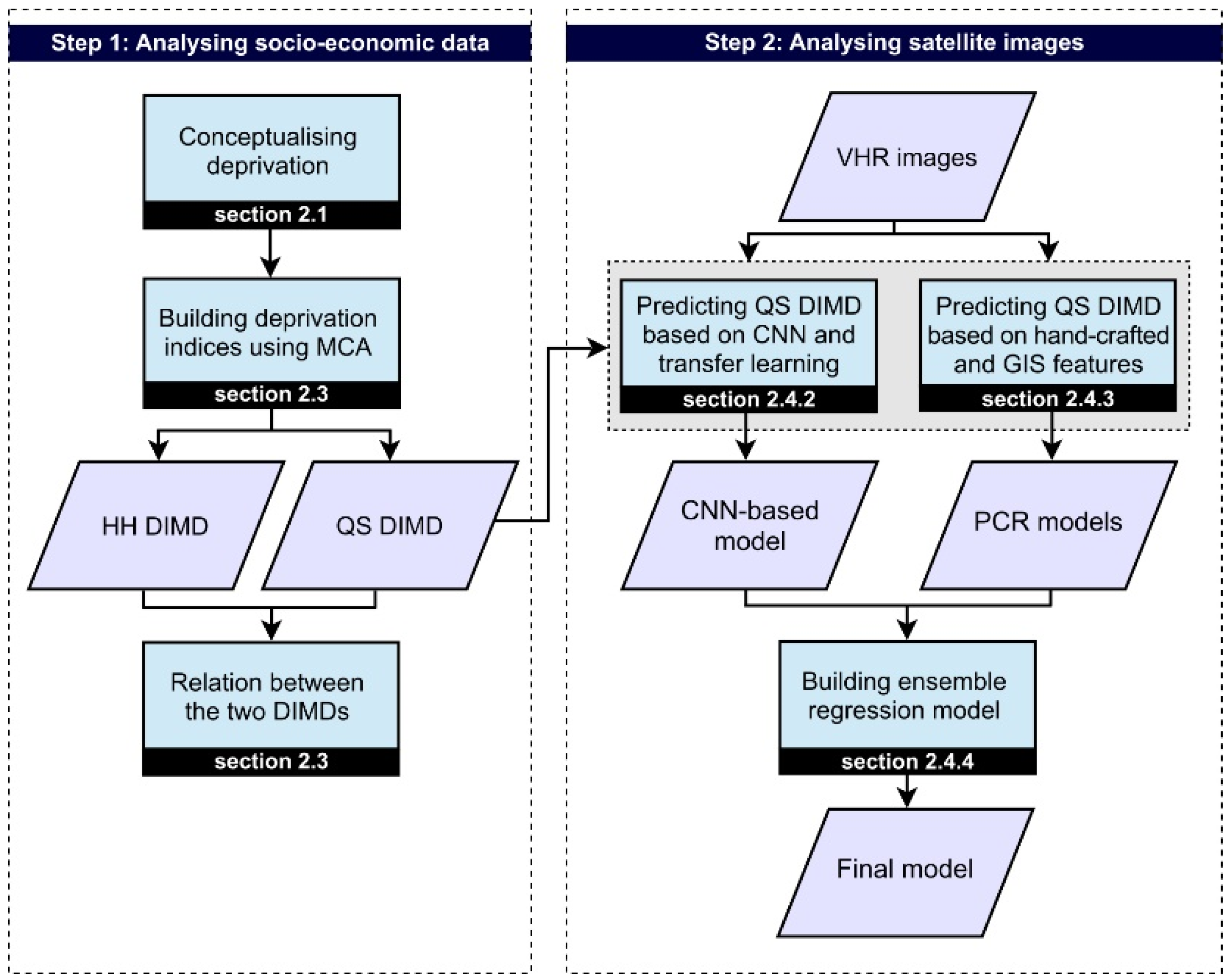
Figure 2.
Framework conceptualizing deprivation. Four main domains of deprivation are adopted from the Index of Multiple Deprivation (IMD) by [34]. The contextual domain is added by this study to bring information about the spatial context. Remote sensing images and GIS layers can capture information about the physical and contextual domains only. Example indicators in each domain are as follows: income (financial domain), education and health (human domain), caste (social domain), constructing materials (physical domain), accessibility to services (contextual domain).

Figure 3.
Available satellite images and slums’ data. Note that between HH and QS samples, 26 are in common, so 26 of the red dots are QS samples as well.
Figure 3.
Available satellite images and slums’ data. Note that between HH and QS samples, 26 are in common, so 26 of the red dots are QS samples as well.

Figure 4.
The process of generating buffer around slum samples and erasing from formal samples (a), all prepared samples (b).
Figure 4.
The process of generating buffer around slum samples and erasing from formal samples (a), all prepared samples (b).

Figure 5.
Steps to classify slums and formal areas using CNNs.

Figure 6.
Shallow CNN architecture. Numbers show the size of each layer, p means pad and s means stride in convolutional layers. ReLU means rectified linear unit activation function, Drop means drop-out layer with the rate of 0.5, FC means fully connected layer, and Soft means softmax classifier.
Figure 6.
Shallow CNN architecture. Numbers show the size of each layer, p means pad and s means stride in convolutional layers. ReLU means rectified linear unit activation function, Drop means drop-out layer with the rate of 0.5, FC means fully connected layer, and Soft means softmax classifier.
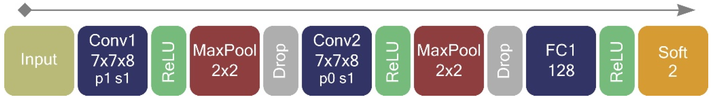
Figure 7.
Deep CNN architecture—Numbers show the size of each layer, p means pad and s means stride in convolutional layers. ReLU means rectified linear unit activation function, Drop means drop-out layer with the rate of 0.5, BNorm means batch normalization layer, FC means fully connected layer, and Soft means softmax classifier.
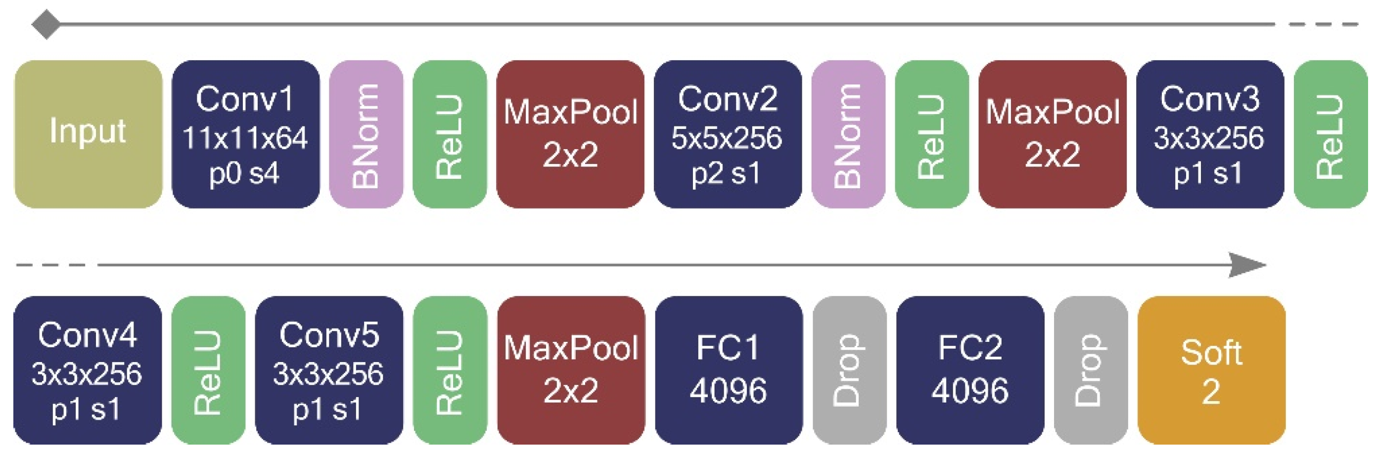
Figure 8.
PCR combinations. Three possibilities for feature combinations, 12 possibilities for a number of components (1 to 12), and three possibilities for model complexity. In total, 108 stepwise principal component regressions are performed.
Figure 8.
PCR combinations. Three possibilities for feature combinations, 12 possibilities for a number of components (1 to 12), and three possibilities for model complexity. In total, 108 stepwise principal component regressions are performed.
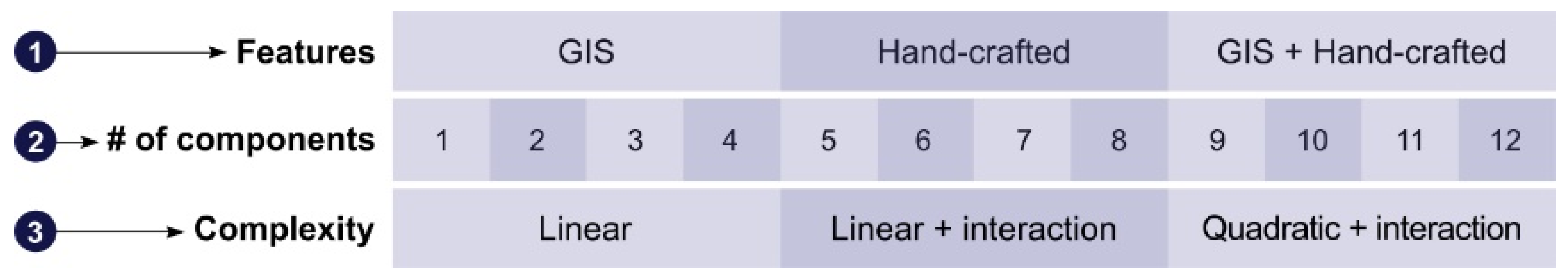
Figure 9.
Squared correlation of HH indicators with the HH DIMD (a), aggregated HH DIMD values into slums with respective standard deviations (b).
Figure 9.
Squared correlation of HH indicators with the HH DIMD (a), aggregated HH DIMD values into slums with respective standard deviations (b).

Figure 10.
QS slums on the map with some ground examples. Sample number 2 shows the common situation of slums in Bangalore as it as a QS DIMD value around zero. Source of the ground photos: Chloe Pottinger Glass, 2017.
Figure 10.
QS slums on the map with some ground examples. Sample number 2 shows the common situation of slums in Bangalore as it as a QS DIMD value around zero. Source of the ground photos: Chloe Pottinger Glass, 2017.

Figure 11.
Results of training CNNs. The best result is obtained by a patch size of 129 and the deep CNN architecture with image augmentation.
Figure 11.
Results of training CNNs. The best result is obtained by a patch size of 129 and the deep CNN architecture with image augmentation.
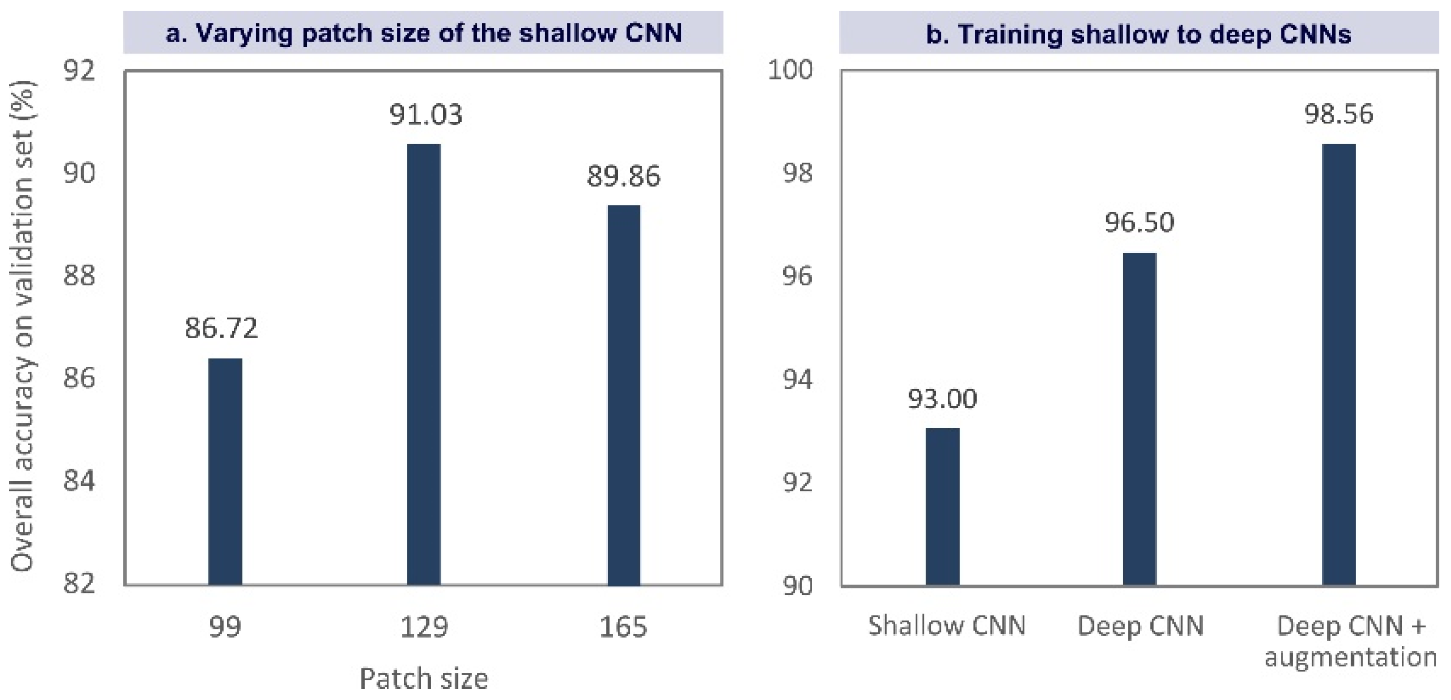
Figure 12.
Per class accuracy with some examples of classified patches.

Figure 13.
Performance of the PCR models. Interaction means allowing the multiplication of the components. The best result is obtained by combining both GIS and hand-crafted image features in a linear regression using 11 components.
Figure 13.
Performance of the PCR models. Interaction means allowing the multiplication of the components. The best result is obtained by combining both GIS and hand-crafted image features in a linear regression using 11 components.

Figure 14.
Plot of QS DIMD and predicted values by the ensemble model.
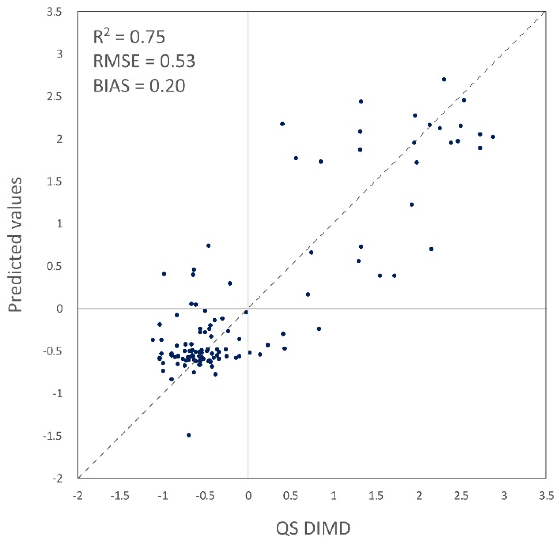
Figure 15.
Worst-off and best-off slums predicted by the model with respective patches. Source of the ground photos: Chloe Pottinger Glass, 2017.
Figure 15.
Worst-off and best-off slums predicted by the model with respective patches. Source of the ground photos: Chloe Pottinger Glass, 2017.
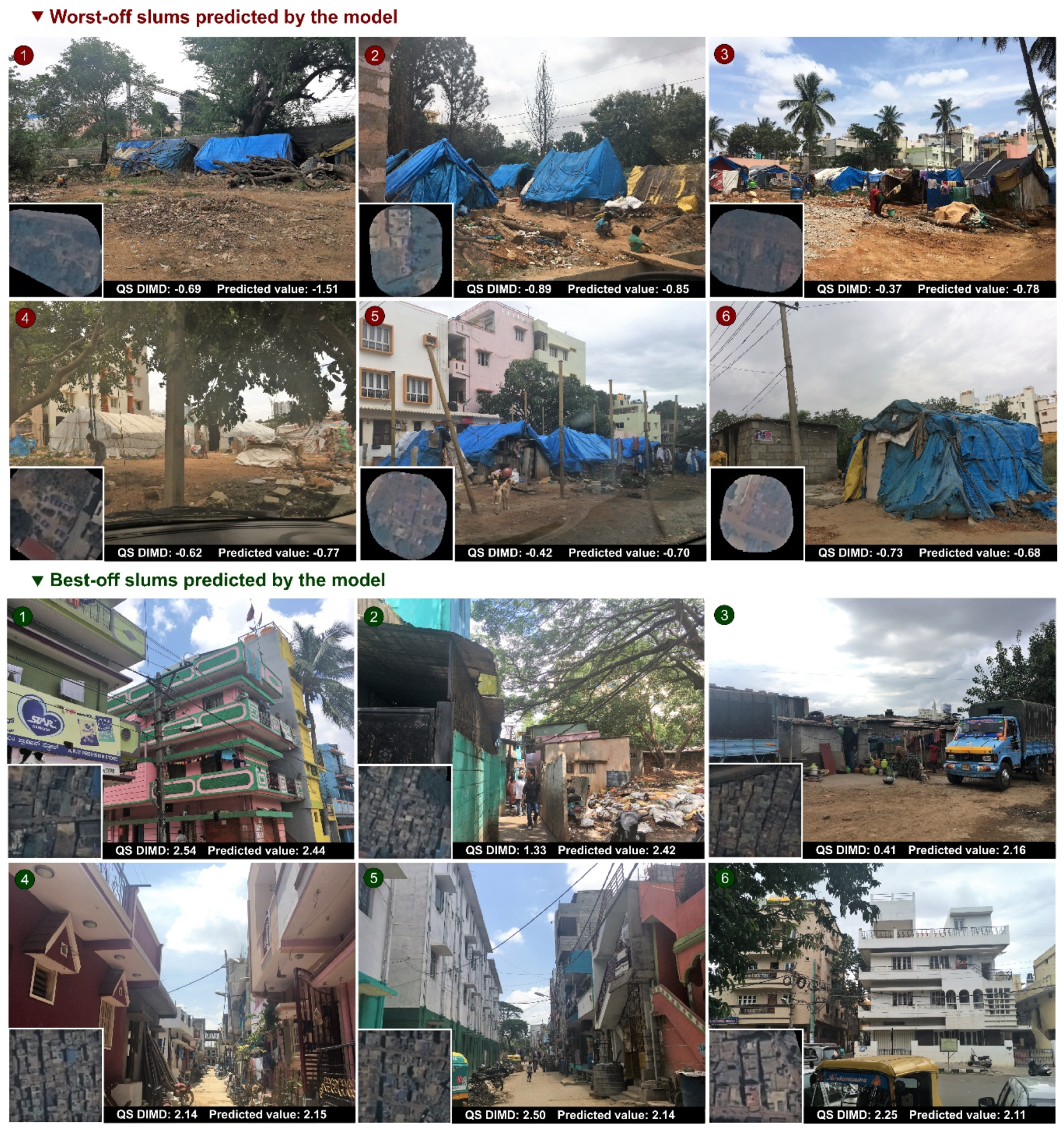
Figure 16.
Standardized residual over predicted values for the created models. CNN-based model (a), principal component regression model combining hand-crafted and GIS features (b), ensemble model (c).
Figure 16.
Standardized residual over predicted values for the created models. CNN-based model (a), principal component regression model combining hand-crafted and GIS features (b), ensemble model (c).


Table 1.
HH and QS indicators. See Supplementary Materials (Sections S1 and S2) for more details about the categories.
Table 1.
HH and QS indicators. See Supplementary Materials (Sections S1 and S2) for more details about the categories.
| Data Set | Indicators |
|---|---|
| HH (16 indicators 118 categories) | Caste, Highest educational level obtained, Dependency rate, Distance to healthcare, Income, Ration Card, Water source quality (summer and other seasons), Toilet facility, Access to electricity, Crowdedness, Dwelling age, Floor material, Wall material, Roof material, Travel time to services |
| QS (35 indicators 109 categories) | Dominant building type, Number of floors, Dominant building footprint size, Wall material, Roof material, Dominant shape of building, Overall state of buildings, Overall building appearance, Open spaces/green spaces, Appearance of open space, Presence of roads, Road pavement, Road material, Road width, Cables for electricity, Presence of footpaths, Footpath material, Streetlight, Pollution (smell, noise, waste), Open sewers, Presence of public toilet, Waterbody, Economic activities, Type of economic activities, Dominant land use around the slum, Feeling safe?, Are people interacting?, Are there vehicles visible?, Temple, Clothes of people, Having jewelry?, Hair of children, Children toys |
Table 2.
CNN hyper-parameters.
| Hyper-Parameter | Value |
|---|---|
| Batch size | 64 |
| Learning rate | Decreases logarithmically from 0.01 to 0.00001 |
| Weight decay | 0.0005 |
| Momentum | 0.9 |
Table 3.
Manually extracted features.
| Feature Name | Specification | # of Features |
|---|---|---|
| Spectral info. | Band mean and standard deviation, NDVI mean and standard deviation | 8 + 2 |
| GLCM | 4 directions [i 0][i i][0 i][−i i]); i = 1,2,3,4; three properties | 16 + 16 + 16 |
| LBP | , , | 10 + 18 + 26 |
| GIS | Transportation: distance to (1) main road, (2) bus stop, (3) railway, (4) railway station; Healthcare: distance to (5) healthcare, (6) pharmacy; Other services: distance to (7) school, (8) leisure activities; Centrality: distance to (9) town hall; Environment: (10) distance to waterbody (11) elevation mean (12) slope mean. | 12 |
Table 4.
Results of training ensemble regression models (numbers show R2 values).
| Linear | Interactions | Quadratic + Interactions | 3rd Degree + Interactions | 4th Degree + Interactions | 5th Degree + Interactions | 6th Degree + Interactions | |
|---|---|---|---|---|---|---|---|
| CNN + hand-crafted + GIS | 0.73 | 0.73 | 0.73 | 0.75 | 0.74 | 0.74 | 0.41 |
| CNN + hand-crafted | 0.67 | 0.67 | 0.65 | 0.38 | 0.62 | −0.23 | <−1.00 |
| CNN + GIS | 0.71 | 0.71 | 0.71 | 0.65 | 0.49 | <−1.00 | <−1.00 |
© 2019 by the authors. Licensee MDPI, Basel, Switzerland. This article is an open access article distributed under the terms and conditions of the Creative Commons Attribution (CC BY) license (http://creativecommons.org/licenses/by/4.0/).
Share and Cite
MDPI and ACS Style
Ajami, A.; Kuffer, M.; Persello, C.; Pfeffer, K. Identifying a Slums’ Degree of Deprivation from VHR Images Using Convolutional Neural Networks. Remote Sens. 2019, 11, 1282. https://doi.org/10.3390/rs11111282
AMA Style
Ajami A, Kuffer M, Persello C, Pfeffer K. Identifying a Slums’ Degree of Deprivation from VHR Images Using Convolutional Neural Networks. Remote Sensing. 2019; 11(11):1282. https://doi.org/10.3390/rs11111282
Chicago/Turabian StyleAjami, Alireza, Monika Kuffer, Claudio Persello, and Karin Pfeffer. 2019. "Identifying a Slums’ Degree of Deprivation from VHR Images Using Convolutional Neural Networks" Remote Sensing 11, no. 11: 1282. https://doi.org/10.3390/rs11111282
Note that from the first issue of 2016, this journal uses article numbers instead of page numbers. See further details here.